Multi-index Stochastic Collocation convergence rates for random PDEs with parametric regularity

Abstract

We analyze the recent Multi-index Stochastic Collocation (MISC) method for computing statistics of the solution of a partial differential equation (PDEs) with random data, where the random coefficient is parametrized by means of a countable sequence of terms in a suitable expansion. MISC is a combination technique based on mixed differences of spatial approximations and quadratures over the space of random data and, naturally, the error analysis uses the joint regularity of the solution with respect to both the variables in the physical domain and parametric variables. In MISC, the number of problem solutions performed at each discretization level is not determined by balancing the spatial and stochastic components of the error, but rather by suitably extending the knapsack-problem approach employed in the construction of the quasi-optimal sparse-grids and Multi-index Monte Carlo methods. We use a greedy optimization procedure to select the most effective mixed differences to include in the MISC estimator. We apply our theoretical estimates to a linear elliptic PDEs in which the log-diffusion coefficient is modeled as a random field, with a covariance similar to a Matérn model, whose realizations have spatial regularity determined by a scalar parameter. We conduct a complexity analysis based on a summability argument showing algebraic rates of convergence with respect to the overall computational work. The rate of convergence depends on the smoothness parameter, the physical dimensionality and the efficiency of the linear solver. Numerical experiments show the effectiveness of MISC in this infinite-dimensional setting compared with the Multi-index Monte Carlo method and compare the convergence rate against the rates predicted in our theoretical analysis.

Keywords: Multilevel, Multi-index Stochastic Collocation, Infinite dimensional integration, Elliptic partial differential equations with random coefficients, Finite element method, Uncertainty quantification, Random partial differential equations, Multivariate approximation, Sparse grids, Stochastic Collocation methods, Multilevel methods, Combination technique.

AMS class: 41A10 (approx by polynomials), 65C20 (models, numerical methods), 65N30 (Finite elements) 65N05 (Finite differences)

1 Introduction

In this work, we analyze and apply the recent MISC method [23] to the approximation of quantities of interest (outputs) from the solutions of linear elliptic partial differential equations (PDEs) with random coefficients. Such equations arise in many applications in which the coefficients of the PDE are described in terms of random variables/fields due either to a lack of knowledge of the system or to its inherent non-predictability. We focus on the weak approximation of the solution of the following linear elliptic ${{\bm{y}}}$-parametric problem:

$$\begin{cases}-\textnormal{div}(a({{\bm{x}}},{{\bm{y}}})\,\nabla u({{\bm{x}}},{{\bm{y}}}))=\varsigma({{\bm{x}}})&\mbox{in}\quad\mathscr{B}\\ u({{\bm{x}}},{{\bm{y}}})\,=\,0&\mbox{on}\quad\partial\mathscr{B}.\end{cases}$$ (1)

Here, $\mathscr{B}\subset\mathbb{R}^{d}$ with $d\in\mathbb{N}$ denotes the “physical domain”, and the operators div and $\nabla$ act with respect to the physical variable, ${{\bm{x}}}\in\mathscr{B}$, only. We assume that $\mathscr{B}$ has a tensor structure, i.e., $\mathscr{B}=\mathscr{B}_{1}\times\mathscr{B}_{2}\times\ldots\times\mathscr{B}_{D}$, with $D\in\mathbb{N}$, $\mathscr{B}_{i}\subset\mathbb{R}^{d_{i}}$ and $\sum_{i=1}^{D}d_{i}=d$, see, e.g., Figures 1(a) and 1(b). This assumption simplifies the analysis detailed in the following, although MISC can be applied to more general domains, such as

• domains obtained by mapping from a reference tensor domain as in Figure 1(c), by suitably extending the approaches in [29, 17];

• non-tensor domains that can be immersed in a tensor bounding box, $\mathscr{B}\subset\hat{\mathscr{B}}=\hat{\mathscr{B}}_{1}\times\hat{\mathscr{B}}_{2}\times\ldots\hat{\mathscr{B}}_{D}$, as in Figure 1(d), whose mesh is obtained as a tensor product of meshes on each component, $\hat{\mathscr{B}}_{i}$, of the bounding box;

• domains that admit a structured mesh, i.e., with a regular connectivity, whose level of refinement in each “direction” can be set independently, as in Figure 1(e);

• domains that can be decomposed in patches satisfying any of the conditions above (observe that the meshes on each patch need not be conforming).

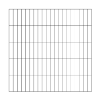
(a) $\mathscr{B}_{1},\mathscr{B}_{2}$ segments

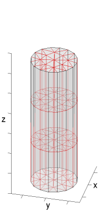
(b) $\mathscr{B}_{1}$ circle, $\mathscr{B}_{2}$ segment

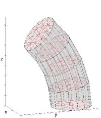
(c) $\mathscr{B}_{1}$ circle, $\mathscr{B}_{2}$ segment

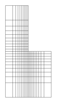
(d) non-tensor $\mathscr{B}$ that can be immersed in a tensor bounding box / divided into tensor subdomains

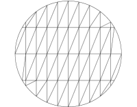
(e) non-tensor $\mathscr{B}$ with a structured mesh

Figure 1: Examples of physical domains on which MISC can be applied: (a) and (b) are within the framework of this work, while treating (c) requires the introduction of a mapping from (b). MISC can also be formulated in non-tensor domains as in (d) and (e), but extending the analysis of the present work to this case is less straightforward and out of the scope of this work.

The parameter ${{\bm{y}}}=\{y_{j}\}_{j\geq 1}$ in (1) is a random sequence whose components are independent and uniformly distributed random variables. More precisely, each $y_{j}$ has support in $[-1,1]$ with measure $\frac{~{}\text{d}\lambda}{2}$, where $~{}\text{d}\lambda$ is the standard Lebesgue measure. We further define $\Gamma=\bigtimes_{j\geq 1}[-1,1]$ (hereafter referred to as the “stochastic domain” or the “parameter space”), with the cylindrical probability measure $~{}\text{d}\mu=\mathop{\bigtimes}_{j\geq 1}\frac{~{}\text{d}\lambda}{2}$, (see, e.g., [5, Chapter 3, Section 5]).

The right-hand side of (1), namely the deterministic function $\varsigma$, does not play a central role in this work and it is assumed to be a smooth function of class $C_{0}^{\infty}(\overline{\mathscr{B}})$, where $\overline{\mathscr{B}}$ denotes the closure of $\mathscr{B}$. This regularity requirement can be relaxed, but we keep it to ease the presentation, since our main goal in this work is to track the effect of the regularity of the coefficient $a$ in (1) on the MISC convergence rate. Here, we focus on the following family of diffusion coefficients:

$$a({{\bm{x}}},{{\bm{y}}})=e^{\kappa({{\bm{x}}},{{\bm{y}}})},\text{ with }\kappa({{\bm{x}}},{{\bm{y}}})=\sum_{j\geq 1}\psi_{j}({{\bm{x}}})y_{j},$$ (2)

where $\{\psi_{j}\}_{j\geq 1}$ is a sequence of functions $\psi_{j}\in C^{t}(\overline{\mathscr{B}})$ for $t\geq 0$ such that $\left\|\psi_{j}\right\|_{L^{\infty}(\mathscr{B})}\to 0$ as $j\to\infty$. Hereafter, without loss of generality, we assume that the sequence $\{\left\|\psi_{j}\right\|_{L^{\infty}(\mathscr{B})}\}_{j\geq 1}$ is ordered in decreasing order. Thanks to a straightforward application of the Lax-Milgram lemma, the well-posedness of (1) in the classical Sobolev space, $V=H^{1}_{0}(\mathscr{B})$, is guaranteed almost surely (a.s.) in $\Gamma$ if two functions, $a_{\min},a_{\max}:\Gamma\to\mathbb{R}$, exist such that

$$0<a_{\min}({{\bm{y}}})\leq a({{\bm{x}}},{{\bm{y}}})\leq a_{\max}({{\bm{y}}})<\infty,\quad\forall{{\bm{x}}}\in\mathscr{B},\,\,\mbox{a.s. in }\Gamma.$$ (3)

Moreover, the equation is well posed in the Bochner space, $L^{q}(\Gamma;V)$, for some $q\geq 1$, (see [1, 8] and the following discussion), provided that sufficiently high moments of the functions $1/a_{\min}$ and $a_{\max}$ are bounded. The goal of our computation is the approximation of an expected value,

$${\mathbb{E}\mspace{-2.0mu}\left[F\right]}={\mathbb{E}\mspace{-2.0mu}\left[\Theta(u)\right]}\in\mathbb{R},$$

where $\Theta$ is a deterministic bounded and linear functional, and $F({{\bm{y}}})=\Theta(u(\cdot,{{\bm{y}}}))$ is a real-valued random variable, $F:\Gamma\rightarrow\mathbb{R}$. To this end, we utilize the Multi-index Stochastic Collocation method (MISC), which we have introduced in a general setting in a previous work [23].

In MISC, we consider a decomposition in terms of tensorized univariate details (i.e., a tensorized hierarchical decomposition), for both the discrete space in which (1) is solved for a fixed value of ${{\bm{y}}}\in\Gamma$ and for the quadrature operator used to approximate the expected value of $F$, relying on the well-established theory of sparse-grid approximation of PDEs on the one hand [42, 6, 7, 22, 27] and of sparse-grid quadrature on the other hand [6, 1, 41, 36, 35, 15]. We use tensor products of such univariate details, obtaining combined deterministic-stochastic, first-order mixed differences to build the MISC estimator of ${\mathbb{E}\mspace{-2.0mu}\left[F\right]}$ by selecting the most effective mixed differences with an optimization approach inspired by the literature on the knapsack problem (see, e.g., [31]). The knapsack approach also was used in [34] to obtain the so-called quasi-optimal sparse grids for PDEs with stochastic coefficients and in [6, 21] in the context of sparse-grid resolution of high-dimensional PDEs.

The resulting method can be seen as an extension of the sparse-grid combination technique for PDEs with stochastic coefficients, as well as a fully sparse, non-randomized version of the Multilevel Monte Carlo method [28, 16, 9, 2]. In particular, MISC differs from other works in the literature that attempt to optimally combine spatial and stochastic resolution levels [38, 39, 26, 30, 4] in two aspects. First, MISC uses combined deterministic-stochastic, first-order differences, which allows us to exploit not only the regularity of the solution with respect to the spatial variables and the stochastic parameters, but also the mixed deterministic-stochastic regularity whenever available. Second, the MISC estimator is built upon an optimization procedure, whereas the above-mentioned works try to balance the error contributions arising from the deterministic and stochastic components of the method without taking into account the corresponding costs. Finally, MISC can also be seen as a sparse-grid quadrature version of the Multi-index Monte Carlo method that was proposed and analyzed in [24].

In [23], MISC was introduced in a general setting and we restricted the analysis to the case of problems of type (1) depending on a finite number of random variables, ${{\bm{y}}}\in\Gamma\subset\mathbb{R}^{N}$, with $N<\infty$. Here, we provide a complexity analysis of MISC in the more challenging case in which the diffusion coefficient $a$ depends on a countable sequence of random variables, $\{y_{j}\}_{j\geq 1}$. Furthermore, we aim at tracking the dependence of the MISC converge rate on the smoothness of the realizations of $a$. This new framework requires that the tools used to prove the complexity of the method be changed: whereas in [23] we used a “direct counting” argument, i.e., we derived a complexity estimate by explicitly summing the work and the error contributions associated with each mixed difference included in the MISC estimator, here we base our proof on a summability argument and on suitable interpolation estimates in mixed regularity spaces. We mention that in [14] an infinite dimensional analysis based on a direct counting argument was recently carried out in the case of hyperbolic cross-type index sets that might arise when quasi-optimizing the work contribution of sparse grid stochastic collocation without spatial discretization.

The rest of this work is organized as follows. Section 2 introduces suitable assumptions and a class of random diffusion coefficients that we consider throughout the work; functional analysis results that are needed for the subsequent analysis of the MISC method are also provided. The MISC method is reviewed in Section 3. A complexity analysis of MISC with an infinite number of random variables is carried out in Section 4, where we provide a general convergence theorem. In Section 5, we discuss the application of MISC to the specific class of diffusion coefficients that we consider here and track the dependence of the convergence rate on the regularity of the diffusion coefficient. Section 6 presents some numerical tests to verify the convergence analysis conducted in the previous section. Finally, Section 7 provides some conclusions and final remarks. In the Appendix, we include some technical results on the summability and regularity properties of certain random fields written in terms of their series expansion.

In the following, $\mathbb{N}$ denotes the set of integer numbers including zero, while $\mathbb{N}_{+}$ denotes the set of positive integer numbers excluding zero. We refer to sequences in $\mathbb{N}^{\mathbb{N}_{+}}$ and $\mathbb{N}_{+}^{\mathbb{N}_{+}}$ as “multi-indices”. Moreover, we often use a vector notation for sequences, i.e., we formally treat sequences as vectors in $\mathbb{N}^{\mathbb{N}_{+}}$ (or $\mathbb{R}^{\mathbb{N}_{+}}$) and mark them with bold type. We employ the following notation, with the understanding that $N<\infty$ for actual vectors and $N=\infty$ for sequences:

• $\bm{1}$ denotes a vector in $\mathbb{N}^{N}$ whose components are all equal to one;

• ${{\bm{e}}}^{N}_{\ell}$ denotes the $\ell$-th canonical vector in $\mathbb{R}^{N}$, i.e., $\left({{\bm{e}}}^{N}_{\ell}\right)_{i}=1$ if $\ell=i$ and zero otherwise; however, for the sake of clarity, we often omit the superscript $N$ whenever it is obvious from context. For instance, if ${{\bm{v}}}\in\mathbb{R}^{N}$, we write ${{\bm{v}}}-{{\bm{e}}}_{1}$ instead of ${{\bm{v}}}-{{\bm{e}}}_{1}^{N}$;

• given ${{\bm{v}}}\in\mathbb{R}^{N}$, $|{{\bm{v}}}|=\sum_{i=1}^{N}v_{i}$, $|{{\bm{v}}}|_{0}$ denotes the number of non-zero components of ${{\bm{v}}}$, $\max({{\bm{v}}})=\max_{i=1,\ldots N}v_{i}$ and $\min({{\bm{v}}})=\min_{i=1,\ldots N}v_{i}$;

• $\mathfrak{L}_{+}$ denotes the set of sequences with positive components with only finitely many elements larger than 1, i.e., $\mathfrak{L}_{+}=\{{{\bm{p}}}\in\mathbb{N}_{+}^{\mathbb{N}_{+}}:|{{\bm{p}}}-\bm{1}|_{0}<\infty\}$;

• given ${{\bm{v}}}\in\mathbb{R}^{N}$ and $f:\mathbb{R}\to\mathbb{R}$, $f({{\bm{v}}})$ denotes the vector obtained by applying $f$ to each component of ${{\bm{v}}}$, $f({{\bm{v}}})=[f(v_{1}),f(v_{2}),\cdots,f(v_{N})]\in\mathbb{R}^{N}$;

• given ${{\bm{v}}},{{\bm{w}}}\in\mathbb{R}^{N}$, the inequality ${{\bm{v}}}>{{\bm{w}}}$ holds true if and only if $v_{i}>w_{i}$ $\forall i=1,\ldots,N$;

• given ${{\bm{v}}}\in\mathbb{R}^{D}$ and ${{\bm{w}}}\in\mathbb{R}^{N}$, we denote their concatenation by $[{{\bm{v}}},{{\bm{w}}}]=(v_{1},\ldots,v_{D},w_{1},\ldots,w_{N})\in\mathbb{R}^{D+N}$;

• given a set with finite cardinality, $\mathcal{G}\subset\mathbb{N}_{+}$, we define the set $\mathbb{N}^{\mathcal{G}}=\{{{\bm{z}}}\in\mathbb{\mathbb{N}}^{\mathbb{N}_{+}}:z_{j}=0\,,\,\forall j\notin\mathcal{G}\}$. We similarly define $\mathbb{R}^{\mathcal{G}}$ and $\mathbb{C}^{\mathcal{G}}$.

2 Functional setting

Even though condition (3) ensures well-posedness of (1) in $V$, we need to make sure that realizations of $u$ a.s. belong to more regular spaces to prove a convergence rate result for MISC. More specifically, due to the classic spatial sparse-grid approximation theory, we need certain conditions on the mixed derivatives of $u$ with respect to the physical coordinates. To this end, we introduce suitable functional spaces (tensor products of fractional Sobolev spaces, see also [19]) and then a “shift” regularity assumption (see Assumption A1 below), i.e., we assume that the regularity of the realizations of $u$ is induced “in a natural way” by the regularity of $a$, of the forcing, $\varsigma$, and of the smoothness of the physical domain, $\mathscr{B}$. In other words, we rule out “pathological”/“ad hoc” examples in which $u$ is very regular despite the data is not, e.g., when the forcing is chosen such that $u\in C^{q}$ for $q>2$ even in the presence of a domain with corners. First, recall the definition of a fractional Sobolev space for $l_{i}\in\mathbb{R}_{+}\setminus\mathbb{N}_{+}$ and $\mathscr{B}_{i}\subset\mathbb{N}^{d_{i}}$:

$$H^{l_{i}}(\mathscr{B}_{i})=\bigg{\{}u\in H^{\lfloor l_{i}\rfloor}(\mathscr{B}_{i}):\sup_{{{{\bm{\alpha}}}}\in\mathbb{N}^{d_{i}},|{{{\bm{\alpha}}}}|=\lfloor l_{i}\rfloor}\int_{\mathscr{B}_{i}}\int_{\mathscr{B}_{i}}\frac{|D^{{{{\bm{\alpha}}}}}u({{\bm{x}}})-D^{{{{\bm{\alpha}}}}}u({{\bm{x}}}^{\prime})|^{2}}{|{{\bm{x}}}-{{\bm{x}}}^{\prime}|^{d_{i}+2(l_{i}-\lfloor l_{i}\rfloor)}}d{{\bm{x}}}d{{\bm{x}}}^{\prime}<\infty\bigg{\}},$$

extending the definition of a standard Sobolev space $H^{l_{i}}(\mathscr{B}_{i})$ for $l_{i}$ integer. The tensorized fractional Sobolev space can then be defined as

$$H^{{{\bm{l}}}}(\mathscr{B})=H^{l_{1}}(\mathscr{B}_{1})\otimes\ldots\otimes H^{l_{D}}(\mathscr{B}_{D})$$

for ${{\bm{l}}}=\left(l_{i}\right)_{i=1}^{D}\in\mathbb{R}^{D}_{+}$. Finally, the mixed fractional Sobolev spaces, that we will need for our analysis, can be defined for each ${{\bm{q}}}\in\mathbb{R}_{+}^{D}$ as

$$\mathcal{H}^{\bm{1}+{{\bm{q}}}}(\mathscr{B})=\bigcap_{j=1}^{D}H^{{{\bm{e}}}_{j}+{{\bm{q}}}}(\mathscr{B}).$$

Observe that, while mixed fractional spaces, $\mathcal{H}^{\bm{1}+{{\bm{q}}}}(\mathscr{B})$, are the proper setting for the forthcoming analysis, we will, for ease of presentation, not look for the most general mixed space in which the solution lives. Instead, we will be content with deducing mixed regularity from inclusions in standard Sobolev spaces, to the point that Assumption A1 will be written in terms of standard Sobolev spaces. For this, we observe that $\mathcal{H}^{\bm{1}}(\mathscr{B})=H^{1}(\mathscr{B})$ holds and in general we have the following inclusion result between standard and mixed fractional Sobolev spaces:

$$u\in H^{1+r}(\mathscr{B})\Rightarrow u\in\mathcal{H}^{\bm{1}+r{{\bm{q}}}}(\mathscr{B})\quad\mbox{for }r\in(0,\infty)\mbox{ and }0<|{{\bm{q}}}|\leq 1.$$ (4)

Before stating precisely the shift-regularity assumption on $u$, we need some more notation and setup. First, observe that this assumption needs to be stated in the complex domain, for reasons that will be made clear later. We therefore extend the diffusion coefficient from $a(\cdot,{{\bm{y}}})$ with ${{\bm{y}}}\in\Gamma$ to $a(\cdot,{{\bm{z}}})$ with ${{\bm{z}}}\in\mathbb{C}^{\mathbb{N}_{+}}$, so that the corresponding solution of (1), $u(\cdot,{{\bm{z}}})$, becomes a $H^{1}_{0}(\mathscr{B})$ function taking values in $\mathbb{C}$, i.e., $u(\cdot,{{\bm{z}}})\in H^{1}_{0}(\mathscr{B},\mathbb{C})$. Since the complex-valued version of problem (1) is well posed as long as there exists $\delta$ such that $\real{a({{\bm{x}}},{{\bm{z}}})}>\delta>0$ for almost every (a.e.) ${{\bm{x}}}\in\mathscr{B}$, and since our approximation method will cover the countable set of parameters ${{\bm{z}}}\in\mathbb{C}^{\mathbb{N}_{+}}$ by multiple subsets of finite cardinality, we define the following region in $\mathbb{C}^{\mathcal{G}}$ for a set of finite cardinality, $\mathcal{G}\subset\mathbb{N}_{+}$:

$$\Sigma_{\mathcal{G},\delta}=\{{{\bm{z}}}\in\mathbb{C}^{\mathcal{G}}:\real{a({{\bm{x}}},{{\bm{z}}})}\geq\delta>0\text{ for a.e. }{{\bm{x}}}\in\mathscr{B}\}.$$ (5)

We are now ready to state the assumption on the link between the regularity of the coefficient, $a$, and the regularity of solution, $u$.

Assumption A1 (Shift assumption).

For a given $\mathscr{B}$, let $\psi_{j}\in C^{t}(\overline{\mathscr{B}})$ (cf. eq. (2)) and $\varsigma\in C^{\infty}_{0}(\overline{\mathscr{B}})$. We assume that there exist $r$ such that $1<r<t$ and that, for any finite set $\mathcal{G}\subset\mathbb{N}_{+}$ and any ${{\bm{z}}}\in\Sigma_{\mathcal{G},\delta}$, the three following conditions hold:

1. $u(\cdot,{{\bm{z}}})\in H^{1+r}(\mathscr{B},\mathbb{C})\cap H^{1}_{0}(\mathscr{B},\mathbb{C})$;

2. $\frac{Du(\cdot,z_{j})}{Dz_{j}}\in H^{1+r}(\mathscr{B},\mathbb{C}),\;\;\forall j\in\mathcal{G}$, where $\frac{Du(\cdot,z_{j})}{Dz_{j}}$ denotes the partial complex derivative of $u$;

3. $\left\|u(\cdot,{{\bm{z}}})\right\|_{H^{1+s}(\mathscr{B},\mathbb{C})}\leq C(\delta,s,\varsigma,\mathscr{B})\left\|a(\cdot,{{\bm{z}}})\right\|_{C^{s}(\overline{\mathscr{B}},\mathbb{C})}$, with $C(\delta,s,\varsigma,\mathscr{B})\to\infty$ for $\delta\to 0$, for every $s=1,\ldots,\lfloor r\rfloor$.

In the following, we will need to ensure that $\left\|u(\cdot,{{\bm{z}}})\right\|_{{H^{1+s}(\mathscr{B,\mathbb{C}})}}$, for $s>0$, is uniformely bounded for all ${{\bm{z}}}$ in certain subregions of the complex plane. Note that this is a stronger condition than what is stated in the previous assumption, where we only assumed pointwise control on the norms of $u$ (i.e., we gave a bound that depends on ${{\bm{z}}}$). In particular, we show at the end of this section that the possibility of having such a uniform bound depends on certain summability properties of the diffusion coefficient. Toward this end, we state the following assumption, which also guarantees the well posedness of Problem (1).

Assumption A2 (Summability of the diffusion coefficient).

For every $s=0,1,\ldots,s_{\max}\leq r$, define the sequences ${{\bm{b}}}_{s}=\{b_{s,j}\}_{j\geq 1}$ where

$$b_{s,j}\,=\,\max_{{{\bm{s}}}\in\mathbb{N}^{d}:|{{\bm{s}}}|\leq s}\left\|D^{{{\bm{s}}}}\psi_{j}\right\|_{L^{\infty}(\mathscr{B})}\;,\qquad j\geq 1.$$ (6)

We assume that an increasing sequence $\{p_{s}\}_{s=0}^{s_{\max}}$ exists such that $0<p_{0}\leq\ldots\leq p_{s_{\max}}<\frac{1}{2}$ and ${{\bm{b}}}_{s}\in\ell^{p_{s}}$, i.e.,

$$\left\|{{\bm{b}}}_{s}\right\|_{\ell^{p_{s}}}^{p_{s}}=\sum_{j\geq 1}b_{s,j}^{p_{s}}<\infty.$$ (7)

We observe that with the above assumption, $b_{s,j}\to 0^{+}$ as $j\to\infty$ and $0\leq b_{0,j}\leq b_{s,j}$ for every $s=0,1,\ldots,s_{\max}$. Moreover, given Assumption A2, we have that ${{\bm{b}}}_{0}\in\ell^{1}$, which, together with the fact that $y_{j}\in[-1,1]$ for $j\geq 1$, guarantees that condition (3) holds and therefore that (1) is well posed in $V$ a.s. in $\Gamma$. Incidentally, we observe that the conditions in Assumption A2 are sufficient but not necessary for condition (3) to hold: indeed, one would only need ${{\bm{b}}}_{s}\in\ell^{2}$ for some integer $s\geq 1$, see Lemma 15 (and Corollary 16 for a specific example) in the Appendix.

As suggested above, the fact that, for a fixed $s$, the sequence ${{\bm{b}}}_{s}$ is $p_{s}$-summable plays a central role in this work. Indeed, if ${{\bm{b}}}_{s}$ is $p_{s}$-summable, we show that $\left\|u(\cdot,{{\bm{z}}})\right\|_{H^{1+s}(\mathscr{B},\mathbb{C})}$ is uniformely bounded with respect to ${{\bm{z}}}$ in a region of the complex plane whose size is proportional to $\left\|{{\bm{b}}}_{s}\right\|_{\ell^{p_{s}}}^{p_{s}}$. We use this fact to show convergence of the MISC method, with the convergence rate dictated by both $p_{0}$ and $p_{s}$. In Theorem 10, we detail how to optimally choose the value of $s$ in the range $0,1,\ldots,s_{\max}$, which is the main result of this work. Restricting the range of values of $s$ by $p_{s}<\frac{1}{2}$ is not crucial; we could relax this to $p_{s}<1$. However, we follow this more stringent assumption because it considerably simplifies some technical steps in the following discussion without affecting the main part of the proof, as we make clear below (see Remark 4). What is important is that $s_{\max}$ might be strictly smaller than $\lfloor r\rfloor$ (i.e., it could happen that ${{\bm{b}}}_{r}$ is $p_{r}$-summable but with $p_{r}>\frac{1}{2}$, or not summable at all); in this case, the line of proof we propose does not fully exploit the regularity of the solution, $u$.

Example 1.

In the numerical section of this work, we consider either $\mathscr{B}=[0,1]$, i.e., $d=D=d_{1}=1$, or $\mathscr{B}=[0,1]^{3}$, i.e., $d=D=3$, $d_{i}=1$ and $\mathscr{B}_{i}=[0,1]$ for $i=1,2,3$. In both cases, we consider the following form for $\kappa({{\bm{x}}},{{\bm{y}}})$:

$$\kappa({{\bm{x}}},{{\bm{y}}})=\sum_{{{\bm{k}}}\in\mathbb{N}^{d}}A_{{{\bm{k}}}}\sum_{{{\bm{\ell}}}\in\{0,1\}^{d}}y_{{{\bm{k}}},{{\bm{\ell}}}}\,\prod_{i=1}^{d}\left(\cos\left({\pi}k_{i}x_{i}\right)\right)^{\ell_{i}}\left(\sin\left({\pi}k_{i}x_{i}\right)\right)^{1-\ell_{i}}.$$ (8)

Observe that it is possible to write $\kappa$ in the form (1) using a bijective mapping from $\{y_{{{\bm{k}}},{{\bm{\ell}}}}\}_{{{\bm{k}}}\in\mathbb{N}^{d},{{\bm{\ell}}}\in\{0,1\}^{d}}$ to $\{y_{j}\}_{j\geq 1}$. We also choose the following values for the $A_{{{\bm{k}}}}$ coefficients:

$$A_{{{\bm{k}}}}{=\left(\sqrt{3}\right)}2^{\frac{|{{\bm{k}}}|_{0}}{2}}(1+|{{\bm{k}}}|^{2})^{-\frac{\nu+d/2}{2}},$$ (9)

for some $\nu>0$. We observe that $\nu$ is a parameter dictating the ${{\bm{x}}}$-regularity of the realizations of $\kappa$, hence of $a$. Moreover, the parameters $\nu$ and $d$ govern the $p_{s}$-summability of the sequence ${{\bm{b}}}_{s}$ for any $s$ and, as a consequence, the overall convergence of the MISC method, as discussed earlier. Section 5 analyzes the summability properties of the series (8).

We conclude this preliminary section by making the shape of the above-mentioned regions more precise in the complex-plane and showing how their sizes depend on the summability properties of $a$. In particular, we will exploit the fact that for any finite set $\mathcal{G}\subset\mathbb{N}_{+}$, for every $s=0,1,\ldots,s_{\max}$ and for any ${{\bm{z}}}\in\mathbb{C}^{\mathcal{G}}$ we have $\kappa(\cdot,{{\bm{z}}})\in C^{s}(\overline{\mathscr{B}},\mathbb{C})$, $\left\|\kappa(\cdot,{{\bm{z}}})\right\|_{C^{s}(\overline{\mathscr{B}},\mathbb{C})}\leq\sum_{j\in\mathcal{G}}|z_{j}|b_{s,j}$ and infer, from the multivariate Faà di Bruno formula (see Appendix A and [13]), that $a(\cdot,{{\bm{z}}})\in C^{s}(\overline{\mathscr{B}},\mathbb{C})$ as well, with the estimate

$$\left\|a(\cdot,{{\bm{z}}})\right\|_{C^{s}(\overline{\mathscr{B}},\mathbb{C})}\leq\frac{s!}{(\log 2)^{s}}\left\|a(\cdot,{{\bm{z}}})\right\|_{C^{0}(\overline{\mathscr{B}},\mathbb{C})}(1+\left\|\kappa(\cdot,{{\bm{z}}})\right\|_{C^{s}(\overline{\mathscr{B}})})^{s},\quad\forall{{\bm{z}}}\in\mathbb{C}^{\mathcal{G}}.$$ (10)

Next, for a given $\zeta>1$, let $\mathcal{E}_{\zeta}$ denote the polyellipse in the complex plane

$$\mathcal{E}_{\zeta}=\bigg{\{}z\in\mathbb{C}:\,\,\real{z}\leq\frac{\zeta+\zeta^{-1}}{2}\cos{\vartheta},\,\,\,\mathfrak{Im}\left[z\right]\leq\frac{\zeta-\zeta^{-1}}{2}\sin{\vartheta},\,\,\vartheta\in[0,2\pi)\bigg{\}}.$$

For any sequence ${{\bm{\zeta}}}=\{\zeta_{j}\}_{j\geq 1}$ with $\zeta_{j}>1$ for every $j\geq 1$ and for any finite set, $\mathcal{G}\subset\mathbb{N}_{+}$, we introduce the Bernstein polyellipse:

$$\mathcal{E}_{{{\bm{\zeta}}}}^{\mathcal{G}}=\{{{\bm{z}}}\in\mathbb{C}^{\mathcal{G}}:z_{j}\in\mathcal{E}_{\zeta_{j}}\mbox{ for all }j\in\mathcal{G}\}.$$ (11)

Lemma 1 (Holomorphic complex continuation of $u$ in $H^{1}_{0}(\mathscr{B};\mathbb{C})$ in a Bernstein polyellipse).

Consider the sequence ${{\bm{b}}}_{0}$ defined in (6). For any $\delta>0$, let $E_{\delta}>2$ be such that

$$\frac{\pi}{E_{\delta}}=-\left\|{{\bm{b}}}_{0}\right\|_{\ell^{1}}-\log\delta+\log\cos\left(\frac{\pi}{E_{\delta}}\right),$$

and consider the sequence ${{\bm{\zeta}}}_{0}=\{\zeta_{0,j}\}_{j\geq 1}$, with

$$\zeta_{0,j} =\tau_{0,j}+\sqrt{\tau_{0,j}^{2}+1}>1$$ (12)

$$\tau_{0,j} =\frac{\pi}{E_{\delta}}\frac{(b_{0,j})^{p_{0}-1}}{\left\|{{\bm{b}}}_{0}\right\|_{\ell^{p_{0}}}^{p_{0}}}\,\,,$$ (13)

with $p_{0}$ as in (7). Then, for any finite set $\mathcal{G}\subset\mathbb{N}_{+}$, the solution, $u$, admits a holomorphic complex continuation, $u:\mathbb{C}^{\mathcal{G}}\rightarrow H^{1}_{0}(\mathscr{B},\mathbb{C})$, in the Bernstein polyellipse, $\mathcal{E}_{{{\bm{\zeta}}}_{0}}^{\mathcal{G}}\subset\Sigma_{\mathcal{G},\delta}$, with

$$\sup_{{{\bm{z}}}\in\mathcal{E}_{{{\bm{\zeta}}}_{0}}^{\mathcal{G}}}\left\|u(\cdot,{{\bm{z}}})\right\|_{H^{1}(\mathscr{B})}\leq C_{0,u}=\frac{\left\|\varsigma\right\|_{H^{-1}(\mathscr{B})}}{\delta}<\infty,$$

with $C_{0,u}$ independent of $\mathcal{G}$.

Proof.

It is well known in the literature that $u:\mathbb{C}^{\mathcal{G}}\rightarrow H^{1}_{0}(\mathscr{B},\mathbb{C})$ is holomorphic in the region $\Sigma_{\mathcal{G},\delta}$ defined in (5) (see, e.g., [1]). To compute the parameters $\{\zeta_{j}\}_{j\in\mathcal{G}}$ of a Bernstein polyellipse contained in $\Sigma_{\mathcal{G},\delta}$, we rewrite $a({{\bm{x}}},{{\bm{z}}})$ as

$$a({{\bm{x}}},{{\bm{z}}}) =\exp\left(\sum_{j\in\mathcal{G}}z_{j}\psi_{j}({{\bm{x}}})\right)=\exp\left(\sum_{j\in\mathcal{G}}\real{z_{j}}\psi_{j}({{\bm{x}}})\right)\exp\left(\sum_{j\in\mathcal{G}}i\mathfrak{Im}\left[z_{j}\right]\psi_{j}({{\bm{x}}})\right)$$

$$=\exp\left(\sum_{j\in\mathcal{G}}\real{z_{j}}\psi_{j}({{\bm{x}}})\right)\left[\cos\left(\sum_{j\in\mathcal{G}}\mathfrak{Im}\left[z_{j}\right]\psi_{j}({{\bm{x}}})\right)+i\sin\left(\sum_{j\in\mathcal{G}}\mathfrak{Im}\left[z_{j}\right]\psi_{j}({{\bm{x}}})\right)\right],$$

so that $\Sigma_{\mathcal{G},\delta}$ can be rewritten as

$$\Sigma_{\mathcal{G},\delta}=\left\{{{\bm{z}}}\in\mathbb{C}^{\mathcal{G}}:\exp\left(\sum_{j\in\mathcal{G}}\real{z_{j}}\psi_{j}({{\bm{x}}})\right)\cos\left(\sum_{j\in\mathcal{G}}\mathfrak{Im}\left[z_{j}\right]\psi_{j}({{\bm{x}}})\right)\geq\delta\,\,\mbox{ for a.e. }{{\bm{x}}}\in\mathscr{B}\right\}.$$

Now, for some $E>2$ that we choose in the following, the two following conditions on ${{\bm{z}}}$ imply that ${{\bm{z}}}\in\Sigma_{\mathcal{G},\delta}$:

$$\begin{cases}\cos\Big{(}\sum_{j\in\mathcal{G}}|\mathfrak{Im}\left[z_{j}\right]|\,b_{0,j}\Big{)}\geq\displaystyle\cos\left(\frac{\pi}{E}\right)\\[10.0pt] \exp\Big{(}-\sum_{j\in\mathcal{G}}|\real{z_{j}}|\,b_{0,j}\Big{)}\geq\displaystyle\frac{\delta}{\cos\left(\frac{\pi}{E}\right)};\end{cases}$$

equivalently, we write

$$\begin{cases}\sum_{j\in\mathcal{G}}|\mathfrak{Im}\left[z_{j}\right]\!|\,b_{0,j}\leq\displaystyle\frac{\pi}{E}\\[8.0pt] \sum_{j\in\mathcal{G}}|\real{z_{j}}|\,b_{0,j}\leq\displaystyle-\log\delta+\log\cos\left(\frac{\pi}{E}\right).\end{cases}$$

For a fixed value of $E$, the equations above define a second region, $\Omega_{\mathcal{G},\delta}$, included in $\Sigma_{\mathcal{G},\delta}$. In turn, the previous conditions are verified if the following conditions, which define a hyper-rectangular region, $\mathcal{R}_{\delta}\subset\Omega_{\mathcal{G},\delta}$, are verified:

$$\begin{cases}\displaystyle|\mathfrak{Im}\left[z_{j}\right]\!|\leq\tau_{0,j}=\frac{\pi(b_{0,j})^{p_{0}-1}}{E\left\|{{\bm{b}}}_{0}\right\|_{\ell^{p_{0}}}^{p_{0}}},\\ \displaystyle|\real{z_{j}}|\leq 1+w_{0,j},\quad\mbox{ with }w_{0,j}=\frac{(b_{0,j})^{p_{0}-1}}{\left\|{{\bm{b}}}_{0}\right\|_{\ell^{p_{0}}}^{p_{0}}}\left(-\left\|{{\bm{b}}}_{0}\right\|_{\ell^{1}}-\log\delta+\log\cos\left(\frac{\pi}{E}\right)\right),\end{cases}$$

provided that $\delta$ and $E$ are such that the quantity $-\left\|{{\bm{b}}}_{0}\right\|_{\ell^{1}}-\log\delta+\log\cos\left(\frac{\pi}{E}\right)$ remains positive. Observe that for sufficiently small $\delta>0$ such $E$ exists, since $f(E)=\log\cos\left(\frac{\pi}{E}\right)$ is a monotonically increasing function, with $f(E)\to-\infty$ for $E\to 2$ and $f(E)\to 0$ for $E\to\infty$, and $-\log\delta$ is positive for sufficiently small $\delta$. In particular, for any $\delta>0$, we choose $E=E_{\delta}$ such that $w_{0,j}=\tau_{0,j}$, which leads to

$$\frac{\pi}{E_{\delta}}=-\left\|{{\bm{b}}}_{0}\right\|_{\ell^{1}}-\log\delta+\log\cos\left(\frac{\pi}{E_{\delta}}\right).$$

We observe that with this choice, $\tau_{0,j}$ (and hence $w_{0,j}$) actually does not depend on $\mathcal{G}$, and that we can define the sequence ${{\bm{\tau}}}_{0}=\{\tau_{0,j}\}_{j\geq 1}$.

We are now in the position to compute the Bernstein polyellipses that touch the boundary of $\mathcal{R}_{\delta}$ on the real and imaginary axes. For the real axis, we have to enforce

$$\frac{\zeta_{j,\text{real}}+\zeta_{j,\text{real}}^{-1}}{2}=1+\tau_{0,j}\Rightarrow\zeta_{j,\text{real}}=1+\tau_{0,j}+\sqrt{(1+\tau_{0,j})^{2}-1},$$

while for the imaginary axis we have to enforce

$$\frac{\zeta_{j,\text{imag}}-\zeta_{j,\text{imag}}^{-1}}{2}=\tau_{0,j}\Rightarrow\zeta_{j,\text{imag}}=\tau_{0,j}+\sqrt{\tau_{0,j}^{2}+1}\,.$$

The proof is concluded by observing that $\zeta_{j,\text{imag}}\leq\zeta_{j,\text{real}}$, i.e., the only polyellipse entirely contained in $\mathcal{R}_{\delta}$, and hence in $\Sigma_{\mathcal{G},\delta}$, is the one touching $\mathcal{R}_{\delta}$ on the imaginary axis, which also implies that the bound $\sup_{{{\bm{z}}}\in\mathcal{E}_{{{\bm{\zeta}}}}^{\mathcal{G}}}\left\|u(\cdot,{{\bm{z}}})\right\|_{H^{1}(\mathscr{B})}\leq C_{0,u}=\frac{\left\|\varsigma\right\|_{H^{-1}(\mathscr{B})}}{\delta}<\infty$ holds independently of $\mathcal{G}$. ∎

Lemma 2 (Holomorphic complex continuation of $u$ in $H^{1+s}(\mathscr{B};\mathbb{C})$ in a Bernstein polyellipse).

For a given $s=1,2,\ldots,s_{\max}$, let ${{\bm{\zeta}}}_{s}=\{\zeta_{s,j}\}_{j\geq 1}$, with

$$\zeta_{s,j} =\tau_{s,j}+\sqrt{\tau_{s,j}^{2}+1}>1,$$ (14)

$$\tau_{s,j} =\frac{\pi(b_{s,j})^{p_{s}-1}}{E_{\delta}\left\|{{\bm{b}}}_{s}\right\|_{\ell^{p_{s}}}^{p_{s}}},$$ (15)

with ${{\bm{b}}}_{s}$ as in (6), $p_{s}$ as in (7), and $E_{\delta}$ as in Lemma 1. For any finite set $\mathcal{G}\subset\mathbb{N}_{+}$, $u:\mathbb{C}^{\mathcal{G}}\rightarrow H^{1+s}(\mathscr{B},\mathbb{C})$ is holomorphic in the Bernstein polyellipse $\mathcal{E}_{{{\bm{\zeta}}}_{s}}^{\mathcal{G}}\subset\Sigma_{\mathcal{G},\delta}$,

$$\sup_{{{\bm{z}}}\in\mathcal{E}_{{{\bm{\zeta}}}_{s}}}\left\|u(\cdot,{{\bm{z}}})\right\|_{H^{1+s}(\mathscr{B})}\leq C_{s,u}=C(\tilde{\delta},s,\varsigma,\mathscr{B})M<\infty$$ (16)

with $M=\frac{s!}{(\log 2)^{s}}e^{K\frac{\pi}{E_{\delta}}}\left(1+K\frac{\pi}{E_{\delta}}\right)^{s}$, $K=\left(2+\frac{1}{\min_{j\geq 1}\tau_{s,j}^{2}}\right)^{1/2}$, $\tilde{\delta}=e^{-K\frac{\pi}{E_{\delta}}}$, $C(\tilde{\delta},s,\varsigma,\mathscr{B})$ as in Assumption A1, and $C_{s,u}$ independent of $\mathcal{G}$.

Proof.

From Assumption A1, $u:\mathbb{C}^{\mathcal{G}}\to H^{1+s}(\mathscr{B},\mathbb{C})$ is complex differentiable for every ${{\bm{z}}}$ in $\Sigma_{\mathcal{G},\varepsilon}$ for any $\varepsilon>0$. It is therefore holomorphic in $\Sigma_{\mathcal{G},\varepsilon}$. Similarly to the previous lemma, we look for a region in which we have an a-priori bound on the $H^{1+s}(\mathscr{B},\mathbb{C})$ norm of $u$ uniformly on ${{\bm{z}}}$. Again from Assumption A1, we have that this is true in the region

$$\Xi_{\mathcal{G},\varepsilon}(M)=\{{{\bm{z}}}\in\mathbb{C}^{\mathcal{G}}:\left\|a(\cdot,{{\bm{z}}})\right\|_{C^{s}(\overline{\mathscr{B}})}\leq M\}\cap\Sigma_{\mathcal{G},\varepsilon}\quad\mbox{ for any }\varepsilon>0.$$

However, contrary to the previous lemma, in this proof, we do not derive the expression of a polyellipse contained in $\Xi_{\mathcal{G},\varepsilon}(M)$, but content ourselves with verifying that the polyellipses, $\mathcal{E}_{\mathcal{G},{{\bm{\zeta}}}_{s}}$, proposed in the statement of the lemma (that we have obtained simply by replacing $b_{0,j}$ with $b_{s,j}$ in (13)) satisfy the requirement, i.e., $\mathcal{E}_{\mathcal{G},{{\bm{\zeta}}}_{s}}\subset\Xi_{\mathcal{G},\tilde{\delta}}(M)$, for every finite set, $\mathcal{G}\subset\mathbb{N}_{+}$, and for a certain $\tilde{\delta}$ that we specify later to control the coercivity of the problem. To this end, let us consider the univariate polyellipse $\mathcal{E}_{\zeta_{s,j}}$. We first prove that this polyellipse is contained in the following complex rectangle:

$$\mathcal{R}_{j}=\{z\in\mathbb{C}:|\real{z}|\leq\sqrt{1+\tau_{s,j}^{2}},\,\,|\mathfrak{Im}\left[z\right]|\leq\tau_{s,j}\}.$$

The bound on the imaginary part of $z$ is a consequence of the choice of the polyellipse in (11) and (14). For the real part, we compute the point $z_{0}$ where the polyellipse intersects the real axis by equating

$$z_{0}= \frac{\zeta_{s,j}+\frac{1}{\zeta_{s,j}}}{2}=\frac{\zeta_{s,j}^{2}+1}{2\zeta_{s,j}}=\frac{\tau_{s,j}^{2}+1+\tau_{s,j}\sqrt{\tau_{s,j}^{2}+1}}{\tau_{s,j}+\sqrt{\tau_{s,j}^{2}+1}}$$

$$=\left(\tau_{s,j}^{2}+1+\tau_{s,j}\sqrt{\tau_{s,j}^{2}+1}\right)\left(\sqrt{\tau_{s,j}^{2}+1}-\tau_{s,j}\right)=\sqrt{1+\tau_{s,j}^{2}}.$$

Furthermore, we observe that $|z|\leq\sqrt{1+2\tau_{s,j}^{2}}\leq K\tau_{s,j}$ for every $z\in\mathcal{R}_{j}$ and some $K>0$; for instance, we could look for the smallest $\tau_{s,j}$, say $\tau_{s,j^{*}}$, choose $K$ accordingly, i.e., such that $(K^{2}-2)\tau_{s,j^{*}}^{2}\geq 1$, and obtain the value in the statement of the lemma. Next, according to (10) and Assumption A2,

$$\left\|a(\cdot,{{\bm{z}}})\right\|_{C^{s}(\overline{\mathscr{B}},\mathbb{C})}\leq\frac{s!}{(\log 2)^{s}}\left\|a(\cdot,{{\bm{z}}})\right\|_{C^{0}(\overline{\mathscr{B}},\mathbb{C})}(1+\left\|\kappa(\cdot,{{\bm{z}}})\right\|_{C^{s}(\overline{\mathscr{B}},\mathbb{C})})^{s}\leq\frac{s!}{(\log 2)^{s}}e^{\sum_{j\in\mathcal{G}}b_{0,j}|z_{j}|}\left(1+\sum_{j\in\mathcal{G}}b_{s,j}|z_{j}|\right)^{s}$$

holds. We finish the proof by observing that for every, ${{\bm{z}}}\in\mathcal{E}_{\mathcal{G},{{\bm{\zeta}}}_{s}}$, we have

$$\sum_{j\in\mathcal{G}}b_{0,j}|z_{j}|\leq\sum_{j\in\mathcal{G}}b_{s,j}|z_{j}|\leq K\sum_{j\in\mathcal{G}}b_{s,j}\tau_{s,j}=K\frac{\pi}{E_{\delta}}\sum_{j\in\mathcal{G}}b_{s,j}\frac{(b_{s,j})^{p_{s}-1}}{\left\|{{\bm{b}}}_{s}\right\|_{\ell^{p_{s}}}^{p_{s}}}\leq K\frac{\pi}{E_{\delta}},$$

which gives uniform control of the norm of $\left\|a(\cdot,{{\bm{z}}})\right\|_{C^{s}(\overline{\mathscr{B}},\mathbb{C})}$ within $\mathcal{E}_{{{\bm{\zeta}}}_{s}}^{\mathcal{G}}$ as required. More precisely, we have

$$\left\|a(\cdot,{{\bm{z}}})\right\|_{C^{s}(\overline{\mathscr{B}},\mathbb{C})}\leq M=\frac{s!}{(\log 2)^{s}}e^{K\frac{\pi}{E_{\delta}}}\left(1+K\frac{\pi}{E_{\delta}}\right)^{s},\quad\forall{{\bm{z}}}\in\mathcal{E}_{\mathcal{G},{{\bm{\zeta}}}_{s}},$$

which together with Assumption A1 gives the desired bound on $\left\|u(\cdot,{{\bm{z}}})\right\|_{H^{1+s}(\mathscr{B})}$ in (16) and

$$\real{a({{\bm{x}}},{{\bm{z}}})}\geq e^{-K\frac{\pi}{E_{\delta}}}=:\tilde{\delta}>0.$$

∎

The following result from [23, 34] is also needed. Since this result is concerned with the finite-dimensional case, i.e., $\mathcal{G}=\{1,2,\ldots,N\}$ and ${{\bm{\zeta}}}\in\mathbb{R}^{N}$, we write, for ease of notation, $\mathcal{E}_{{{\bm{\zeta}}}}$ instead of $\mathcal{E}_{{{\bm{\zeta}}}}^{\mathcal{G}}$, i.e., $\mathcal{E}_{{{\bm{\zeta}}}}=\{{{\bm{z}}}\in\mathbb{C}^{N}:z_{j}\in\mathcal{E}_{\zeta_{j}}\mbox{ for }j=1,2,\ldots,N\}$.

Lemma 3 (Chebyshev expansion of a holomorphic function).

Given $q_{j}\in\mathbb{N}$, let $\phi_{q_{j}}$ be the family of Chebyshev polynomials of the first kind on $[-1,1]$, i.e., $|\phi_{q_{j}}(y)|\leq 1$ for all $y\in[-1,1]$, and, for $N\in\mathbb{N}_{+}$ and any ${{\bm{p}}}\in\mathbb{N}^{N}$, let $\Phi_{{\bm{p}}}({{\bm{y}}})=\prod_{j=1}^{N}\phi_{p_{j}}(y_{j})$. If $f:[-1,1]^{N}\to\mathbb{R}$ admits a holomorphic complex extension in a Bernstein polyellipse, $\mathcal{E}_{{{\bm{\zeta}}}}$, for some ${{\bm{\zeta}}}\in(1,\infty)^{N}$ and if there exists $0<C_{f}<\infty$ such that $\sup_{{{\bm{z}}}\in\mathcal{E}_{{{\bm{\zeta}}}}}|f({{\bm{z}}})|\leq C_{f}$, then $f$ admits the following Chebyshev expansion:

$$f({{\bm{y}}})=\sum_{{{\bm{p}}}\in\mathbb{N}^{N}}f_{{\bm{p}}}\Phi_{{\bm{p}}}({{\bm{y}}}),$$

$$f_{{\bm{p}}}=\frac{1}{\int_{[-1,1]^{N}}\Phi_{{\bm{p}}}^{2}({{\bm{y}}})\varrho_{C}({{\bm{y}}})d{{\bm{y}}}}\int_{[-1,1]^{N}}f({{\bm{y}}})\Phi_{{\bm{p}}}({{\bm{y}}})\varrho_{C}({{\bm{y}}})d{{\bm{y}}},\quad\varrho_{C}({{\bm{y}}})=\prod_{j=1}^{N}\left(\sqrt{1-y_{j}^{2}}\right)^{-1},$$

which converges uniformely in $\mathcal{E}_{{{\bm{\zeta}}}}$. Moreover the following bound on the coefficients $f_{{\bm{p}}}$ holds:

$$|f_{{\bm{p}}}|\leq\sup_{{{\bm{z}}}\in\mathcal{E}_{{{\bm{\zeta}}}}}|f({{\bm{z}}})|2^{|{{\bm{p}}}|_{0}}\prod_{j=1}^{N}\zeta_{j}^{-p_{j}},$$

where $|{{\bm{p}}}|_{0}$ denotes the number of non-zero elements of ${{\bm{p}}}$.

3 The Multi-index Stochastic Collocation method

In this section, we introduce approximations of ${\mathbb{E}\mspace{-2.0mu}\left[F\right]}$ along the deterministic and stochastic dimensions and their decomposition in terms of tensorizations of univariate difference operators. We then recall the so-called mixed difference operators and the construction of the MISC estimator, that was first introduced in [23] in a general setting.

3.1 Approximation along the deterministic and stochastic variables

A tensorized deterministic solver.

Let $\{\mathbb{T}_{i}\}_{i=1}^{D}$ be the triangulations/meshes of each of the subdomains $\{\mathscr{B}_{i}\}_{i=1}^{D}$ composing the domain $\mathscr{B}$; denote by $\{h_{i}\}_{i=1}^{D}$ the mesh-size on the mesh $\mathbb{T}_{i}$; and let $\bigotimes_{i=1}^{D}\mathbb{T}_{i}$ be the mesh for $\mathscr{B}$. Then, consider a numerical method for the approximation of the solution of (1) for a fixed value of the random variables, ${{\bm{y}}}$, based on such a mesh, e.g., finite differences, finite volumes, tensorized finite elements, or $h$-refined splines, such as those used in the isogeometric context. The values of $h_{i}$ are actually given as functions of a positive integer value, $\alpha\geq 1$, referred to as a “deterministic discretization level”, i.e., $h_{i}=h_{i}(\alpha)$. Observe that, in a more general setting, the mesh-size needs not be a constant value over the subdomain $\mathscr{B}_{i}$ and could be for instance the result of a grading function intended to refine subregions of $\mathscr{B}_{i}$ as in Figure 1(d) (see also [25, Remark 2.2] for further comments on locally refined meshes in the context of Multi-Level Monte Carlo methods). In this work, we restrict ourselves to constant $h$ for ease of presentation. Given a multi-index, ${{{\bm{\alpha}}}}\in\mathbb{N}^{D}_{+}$, we denote by $u^{{{\bm{\alpha}}}}({{\bm{x}}},{{\bm{y}}})$ the approximation of $u$ obtained by setting $h_{i}=h_{i}(\alpha_{i})$ and use notation $F^{{{\bm{\alpha}}}}({{\bm{y}}})=\Theta[u^{{{\bm{\alpha}}}}(\cdot,{{\bm{y}}})]$. More specifically, in the following we will consider

$$h_{i}=h_{0,i}2^{-\alpha_{i}},\quad\mbox{for }i=1,\ldots,D$$ (17)

and a method obtained by tensorizing piecewise multi-linear finite element spaces on each mesh, $\{\mathbb{T}_{i}\}_{i=1}^{D}$, discretizing each $\{\mathscr{B}_{i}\}_{i=1}^{D}$.

As already mentioned in the previous section, MISC could also be applied to more general domains, such as those discussed in Figure 1, as long as some kind of “tensor structure” can be induced from the shape of the domain to the solver of the deterministic problem and the vector ${{{\bm{\alpha}}}}$ determines the refinement level of each component of such a tensor structure. The reason why we need such tensor strucure will be made clear when we introduce the classic sparse-grids approach to solve the problem. For non-tensorial domains, we can always set $D=1$ and consider an unstructured mesh for the whole domain, $\mathscr{B}$, having only one discretization level $\alpha\in\mathbb{N}_{+}$. In this way, we give up the sparse-grid approach on the deterministic part of the problem and obtain a variant of the Multi-Level Stochastic Collocation method discussed in [38, 39], yet with a different algorithm for combining spatial and stochastic discretizations. See Remark 1 stated next and [23] for additional discussion on this aspect.

It would be straightforward to extend this setting to discretization methods based on degree-elevation rather than on mesh-refinement, such as spectral methods, $p$-refined finite elements or $p$- and $k$-refined splines. However, here we limit ourselves to the setting defined above. It would also be possible to include time-dependent problems in this framework, but in this case we might need to take care of possible constraints on discretization parameters, such as CFL conditions; a broader generalization could also include “non-physical” parameters such as tolerances for numerical solvers. Finally, more general problems, e.g., those depending on random variables with probability distributions other than uniform distributions or with uncertain boundary conditions and/or forcing terms could also be addressed with suitable modifications of the MISC methodology.

Tensorized quadrature formulae for expected value approximation.

Similarly to what was presented for the deterministic problem, we base our approximation of the expected value of $F^{{{\bm{\alpha}}}}({{\bm{y}}})$ on a tensorization of quadrature formulae over the stochastic domain, $\Gamma$. Assumptions A1 and A2 guarantee that $F^{{{\bm{\alpha}}}}({{\bm{y}}})$ is actually a continuous function, even holomorphic, over $\Gamma$. A quadrature approach is thus sound.

Let $C^{0}([-1,1])$ be the set of real-valued continuous functions over $[-1,1]$, $\beta\in\mathbb{N}_{+}$ be referred to as a “stochastic discretization level”, and $m:\mathbb{N}\rightarrow\mathbb{N}$ be a strictly increasing function with $m(0)=0$ and $m(1)=1$, that we call a “level-to-nodes function”. At level $\beta$, we consider a set of $m(\beta)$ distinct quadrature points in $[-1,1]$, $\mathscr{P}^{m(\beta)}=\{y_{\beta}^{1},y_{\beta}^{2},\ldots,y_{\beta}^{m(\beta)}\}\subset[-1,1]$, and a set of quadrature weights, $\mathcal{W}^{m(\beta)}=\{\varpi_{\beta}^{1},\varpi_{\beta}^{2},\ldots,\varpi_{\beta}^{m(\beta)}\}$. We then define the quadrature operator as

$$Q^{m(\beta)}:C^{0}([-1,1])\rightarrow\mathbb{R},\qquad Q^{m(\beta)}[f]=\sum_{j=1}^{m(\beta)}f(y_{\beta}^{j})\varpi_{\beta}^{j}.$$ (18)

The quadrature weights are selected such that $Q^{m(\beta)}[y^{k}]=\int_{-1}^{1}\frac{y^{k}}{2}dy,\quad\forall\,k=0,1,\ldots,m(\beta)-1$. The quadrature points are chosen to optimize the convergence properties of the quadrature error (the specific choice of quadrature points is discussed later in this section). In particular, for symmetry reasons, we define the trivial operator $Q^{1}[f]=f(0)\,,\,\forall f\in C^{0}([-1,1])$.

Defining a quadrature operator over $\Gamma$ is more delicate, since $\Gamma$ is defined as a countable tensor product of intervals. To this end, we follow [37] and define, for any finitely supported multi-index ${{{\bm{\beta}}}}\in\mathfrak{L}_{+}$,

$$\mathscr{Q}^{m({{{\bm{\beta}}}})}:\Gamma\rightarrow\mathbb{R},\quad\mathscr{Q}^{m({{{\bm{\beta}}}})}=\bigotimes_{j\geq 1}Q^{m(\beta_{j})},$$

where the $j$-th quadrature operator is understood to act only on the $j$-th variable of $f$, and the tensor product is well defined since it is composed of finitely many non-trivial factors (see [37] again). In practice, the value of $\mathscr{Q}^{m({{{\bm{\beta}}}})}[f]$ can be obtained by considering the tensor grid $\mathscr{T}^{m({{{\bm{\beta}}}})}=\bigtimes_{j\geq 1}\mathscr{P}^{m(\beta_{j})}$ with cardinality $\#\mathscr{T}^{m({{{\bm{\beta}}}})}=\prod_{j\geq 1}m(\beta_{j})$ and computing

$$\mathscr{Q}^{m({{{\bm{\beta}}}})}[f]=\sum_{j=1}^{\#\mathscr{T}^{m({{{\bm{\beta}}}})}}f(\widehat{{{\bm{y}}}}_{j})w_{j},$$

where $\widehat{{{\bm{y}}}}_{j}\in\mathscr{T}^{m({{{\bm{\beta}}}})}$ and $w_{j}$ are (infinite) products of weights of the univariate quadrature rules. Notice that having $m(1)=1$ is essential in this construction so that the cardinality of $\mathscr{T}^{m({{{\bm{\beta}}}})}$ is finite for any ${{{\bm{\beta}}}}\in\mathfrak{L}_{+}$ and $\varpi_{\beta_{j}}^{1}=1$ whenever $\beta_{j}=1$. All weights, $w_{j}$, are thus bounded.

Coming back to the choice of the univariate quadrature points, it is recommended, for optimal performance, that they are chosen according to the underlying measure, $~{}\text{d}\lambda/2$. Moreover, since we aim at a hierarchical decomposition of the operator, $\mathscr{Q}^{m({{{\bm{\beta}}}})}$, it is useful (although not necessary, see e.g., [34]) that the nodes be nested collocation points, i.e., $\mathscr{P}^{m(\beta)}\subset\mathscr{P}^{m(\beta+1)}$ for any $\beta\geq 1$. Thus, we consider Clenshaw-Curtis points that are defined as

$$y_{\beta}^{j}=\cos\left(\frac{(j-1)\pi}{m(\beta)-1}\right),\quad 1\leq j\leq m(\beta).$$ (19)

Clenshaw-Curtis points are nested provided that the level-to-nodes function is defined as

$$m(0)=0,\,\,m(1)=1,\,\,m(\beta)=2^{\beta-1}+1.$$ (20)

We close this section by mentioning that another family of nested points for uniform measures available in the literature is the Leja points, whose performance is equivalent to that of Clenshaw-Curtis points for quadrature purposes. See, e.g., [10, 33, 32, 37] and references therein for definitions and comparison.

3.2 Construction of the MISC estimator

It is straightforward to see that a direct approximation, ${\mathbb{E}\mspace{-2.0mu}\left[F\right]}\approx\mathscr{Q}^{m({{{\bm{\beta}}}})}[F^{{{\bm{\alpha}}}}]$, is not a viable option in practical cases, due to the well-known “curse of dimensionality” effect. In [23], we proposed to use MISC as a computational strategy to combine spatial and stochastic discretizations in such a way as to obtain an effective approximation scheme for ${\mathbb{E}\mspace{-2.0mu}\left[F\right]}$.

MISC is based on a classic sparsification approach in which approximations like $\mathscr{Q}^{m({{{\bm{\beta}}}})}[F^{{{\bm{\alpha}}}}]$ are decomposed in a hierarchy of operators. Only the most important of these operators are retained in the approximation. In more detail, let us denote for brevity $\mathscr{Q}^{m({{{\bm{\beta}}}})}[F^{{{\bm{\alpha}}}}]=F_{{{{\bm{\alpha}}}},{{{\bm{\beta}}}}}$ and introduce the first-order difference operators for the deterministic and stochastic discretization operators, denoted respectively by $\Delta_{i}^{\textnormal{det}}$ with $1\leq i\leq D$ and $\Delta_{j}^{\textnormal{stoc}}$ with $j\geq 1$:

$$\Delta_{i}^{\textnormal{det}}[F_{{{{\bm{\alpha}}}},{{{\bm{\beta}}}}}]=\begin{cases}F_{{{{\bm{\alpha}}}},{{{\bm{\beta}}}}}-F_{{{{\bm{\alpha}}}}-{{\bm{e}}}_{i},{{{\bm{\beta}}}}},&\text{if }\alpha_{i}>1,\\ F_{{{{\bm{\alpha}}}},{{{\bm{\beta}}}}}&\text{if }\alpha_{i}=1,\end{cases}$$

$$\Delta_{j}^{\textnormal{stoc}}[F_{{{{\bm{\alpha}}}},{{{\bm{\beta}}}}}]=\begin{cases}F_{{{{\bm{\alpha}}}},{{{\bm{\beta}}}}}-F_{{{{\bm{\alpha}}}},{{{\bm{\beta}}}}-{{\bm{e}}}_{j}},&\text{if }\beta_{j}>1,\\ F_{{{{\bm{\alpha}}}},{{{\bm{\beta}}}}}&\text{if }\beta_{j}=1.\end{cases}$$

As a second step, we define the so-called mixed difference operators,

$${{\bm{\Delta}}}^{\textnormal{det}}[F_{{{{\bm{\alpha}}}},{{{\bm{\beta}}}}}]=\bigotimes_{i=1}^{D}\Delta_{i}^{\textnormal{det}}[F_{{{{\bm{\alpha}}}},{{{\bm{\beta}}}}}]=\Delta_{1}^{\textnormal{det}}\left[\,\Delta_{2}^{\textnormal{det}}\left[\,\cdots\Delta_{D}^{\textnormal{det}}\left[F_{{{{\bm{\alpha}}}},{{{\bm{\beta}}}}}\right]\,\right]\,\right]=\sum_{{{\bm{i}}}\in\{0,1\}^{D}}(-1)^{|{{\bm{i}}}|}F_{{{{\bm{\alpha}}}}-{{\bm{i}}},{{{\bm{\beta}}}}},$$ (21)

$${{\bm{\Delta}}}^{\textnormal{stoc}}[F_{{{{\bm{\alpha}}}},{{{\bm{\beta}}}}}]=\bigotimes_{j\geq 1}\Delta_{j}^{\textnormal{stoc}}[F_{{{{\bm{\alpha}}}},{{{\bm{\beta}}}}}]=\sum_{{{\bm{j}}}\in\{0,1\}^{\mathbb{N}_{+}}}(-1)^{|{{\bm{j}}}|}F_{{{{\bm{\alpha}}}},{{{\bm{\beta}}}}-{{\bm{j}}}}\,,$$ (22)

with the convention that $F_{{{\bm{v}}},{{\bm{w}}}}=0$ whenever a component of ${{\bm{v}}}$ or ${{\bm{w}}}$ is zero. Notice that, since ${{{\bm{\beta}}}}$ has finitely many components larger than 1, the sum on the right-hand side of (22) contains only a finite number of terms. Finally, letting

$${{\bm{\Delta}}}[F_{{{{\bm{\alpha}}}},{{{\bm{\beta}}}}}]={{\bm{\Delta}}}^{\textnormal{stoc}}[{{\bm{\Delta}}}^{\textnormal{det}}[F_{{{{\bm{\alpha}}}},{{{\bm{\beta}}}}}]],$$ (23)

we define the Multi-index Stochastic Collocation (MISC) estimator of ${\mathbb{E}\mspace{-2.0mu}\left[F\right]}$ as

$$\mathscr{M}_{\mathcal{I}}[F]=\sum_{[{{{\bm{\alpha}}}},{{{\bm{\beta}}}}]\in\mathcal{I}}{{\bm{\Delta}}}[F_{{{{\bm{\alpha}}}},{{{\bm{\beta}}}}}]=\sum_{[{{{\bm{\alpha}}}},{{{\bm{\beta}}}}]\in\mathcal{I}}c_{{{{\bm{\alpha}}}},{{{\bm{\beta}}}}}F_{{{{\bm{\alpha}}}},{{{\bm{\beta}}}}},\quad c_{{{{\bm{\alpha}}}},{{{\bm{\beta}}}}}=\sum_{\begin{subarray}{c}[{{\bm{i}}},{{\bm{j}}}]\in\{0,1\}^{D+\mathbb{N}}\\[1.0pt] [{{{\bm{\alpha}}}}+{{\bm{i}}},{{{\bm{\beta}}}}+{{\bm{j}}}]\in\mathcal{I}\end{subarray}}(-1)^{|[{{\bm{i}}},{{\bm{j}}}]|_{0}},$$ (24)

where $\mathcal{I}\subset\mathbb{N}_{+}^{D}\times\mathfrak{L}_{+}$. The second form of the MISC estimator is known as the “combination technique”, since it expresses the MISC approximation as a linear combination of a number of tensor approximations, $F_{{{{\bm{\alpha}}}},{{{\bm{\beta}}}}}$, and might be useful for the practical implementation of the method; we observe in particular that many of its coefficients, $c_{{{{\bm{\alpha}}}},{{{\bm{\beta}}}}}$, are zero.

The effectiveness of MISC crucially depends on the choice of the index set, $\mathcal{I}$. Given the hierarchical structure of MISC, a natural requirement is that $\mathcal{I}$ should be downward closed, i.e.,

$$\forall\,[{{{\bm{\alpha}}}},{{{\bm{\beta}}}}]\in\mathcal{I},\quad\begin{cases}[{{{\bm{\alpha}}}}-{{\bm{e}}}_{i},{{{\bm{\beta}}}}]\in\mathcal{I}\mbox{ for all }1\leq i\leq D\mbox{ such that }\alpha_{i}>1,\\ [{{{\bm{\alpha}}}},{{{\bm{\beta}}}}-{{\bm{e}}}_{j}]\in\mathcal{I}\mbox{ for all }j\geq 1\mbox{ such that }\beta_{j}>1\end{cases}$$

(see also [34, 40, 6]). In addition to this general constraint, in [23] we have detailed a procedure to derive an efficient set, $\mathcal{I}$, based on an optimization technique inspired by the Dantzig algorithm for the approximate solution of the knapsack problem (see [31]). In the following, we briefly summarize this procedure and refer to [23] as well as to [34, 3, 6] for a thorough discussion on the similarities between this procedure and the Dantzig algorithm.

The first step of our optimized construction consists of introducing the “work contribution”, $\Delta W_{{{{\bm{\alpha}}}},{{{\bm{\beta}}}}}$, and “error contribution”, $\Delta E_{{{{\bm{\alpha}}}},{{{\bm{\beta}}}}}$, for each operator, ${{\bm{\Delta}}}[F_{{{{\bm{\alpha}}}},{{{\bm{\beta}}}}}]$. The work contribution measures the computational cost (measured, e.g., as a function of the total number of degrees of freedom, or in terms of computational time) required to add ${{\bm{\Delta}}}[F_{{{{\bm{\alpha}}}},{{{\bm{\beta}}}}}]$ to $\mathscr{M}_{\mathcal{I}}[F]$, i.e.,

$$\Delta W_{{{{\bm{\alpha}}}},{{{\bm{\beta}}}}}={\mathrm{Work}\mspace{-2.0mu}\left[\mathscr{M}_{\mathcal{I}\cup\{[{{{\bm{\alpha}}}},{{{\bm{\beta}}}}]\}}\right]}-{\mathrm{Work}\mspace{-2.0mu}\left[\mathscr{M}_{\mathcal{I}}\right]}={\mathrm{Work}\mspace{-2.0mu}\left[{{\bm{\Delta}}}[F_{{{{\bm{\alpha}}}},{{{\bm{\beta}}}}}]\right]}.$$ (25)

Similarly, the error contribution measures how much the error, $|{\mathbb{E}\mspace{-2.0mu}\left[F\right]}-\mathscr{M}_{\mathcal{I}}[F]|$, would decrease if the operator ${{\bm{\Delta}}}[F_{{{{\bm{\alpha}}}},{{{\bm{\beta}}}}}]$ were added to $\mathscr{M}_{\mathcal{I}}[F]$,

$$\Delta E_{{{{\bm{\alpha}}}},{{{\bm{\beta}}}}}=\left|\mathscr{M}_{\mathcal{I}\cup\{[{{{\bm{\alpha}}}},{{{\bm{\beta}}}}]\}}[F]-\mathscr{M}_{\mathcal{I}}[F]\right|=\left|{{\bm{\Delta}}}[F_{{{{\bm{\alpha}}}},{{{\bm{\beta}}}}}]\right|.$$ (26)

We observe that the following decompositions of the total work and error of the MISC estimator hold:

$${\mathrm{Work}\mspace{-2.0mu}\left[\mathscr{M}_{\mathcal{I}}\right]}=\sum_{[{{{\bm{\alpha}}}},{{{\bm{\beta}}}}]\in\mathcal{I}}\Delta W_{{{{\bm{\alpha}}}},{{{\bm{\beta}}}}},$$ (27)

$$|{\mathbb{E}\mspace{-2.0mu}\left[F\right]}-\mathscr{M}_{\mathcal{I}}[F]|=\left|{\sum_{[{{{\bm{\alpha}}}},{{{\bm{\beta}}}}]\notin\mathcal{I}}{{\bm{\Delta}}}[F_{{{{\bm{\alpha}}}},{{{\bm{\beta}}}}}]}\right|\leq\sum_{[{{{\bm{\alpha}}}},{{{\bm{\beta}}}}]\notin\mathcal{I}}\left|{{{\bm{\Delta}}}[F_{{{{\bm{\alpha}}}},{{{\bm{\beta}}}}}]}\right|=\sum_{[{{{\bm{\alpha}}}},{{{\bm{\beta}}}}]\notin\mathcal{I}}\Delta E_{{{{\bm{\alpha}}}},{{{\bm{\beta}}}}}.$$ (28)

Although it would be tempting to define $\mathcal{I}$ as the set of couples $[{{{\bm{\alpha}}}},{{{\bm{\beta}}}}]$ with the largest error contribution, this choice could be far from optimal in terms of computational cost. As suggested in the literature on the knapsack problem (see [31]), the benefit-to-cost ratio should be taken into account in the decision (see also [23, 34, 3, 6, 21]). More precisely, we propose to build the MISC estimator by first assessing the so-called “profit” of each operator ${{\bm{\Delta}}}[F_{{{{\bm{\alpha}}}},{{{\bm{\beta}}}}}]$, i.e., the quantity

$$P_{{{{\bm{\alpha}}}},{{{\bm{\beta}}}}}=\frac{\Delta E_{{{{\bm{\alpha}}}},{{{\bm{\beta}}}}}}{\Delta W_{{{{\bm{\alpha}}}},{{{\bm{\beta}}}}}}.$$

Then we build an index set for the MISC estimator:

$$\mathcal{I}=\mathcal{I}(\epsilon)=\left\{[{{{\bm{\alpha}}}},{{{\bm{\beta}}}}]\in\mathbb{N}_{+}^{D}\times\mathfrak{L}_{+}\>:\>P_{{{{\bm{\alpha}}}},{{{\bm{\beta}}}}}\geq\epsilon\right\},$$ (29)

for a suitable $\epsilon>0$. We observe that the obtained set is not necessarily downward-closed; we have to enforce this condition a posteriori. Obviously, $\Delta E_{{{{\bm{\alpha}}}},{{{\bm{\beta}}}}}$ and $\Delta W_{{{{\bm{\alpha}}}},{{{\bm{\beta}}}}}$ are not, in general, at our disposal. In practice, we base the construction of the MISC estimator on a-priori bounds for such quantities. More precisely, we derive a-priori ansatzes for these bounds from theoretical considerations and then fit the constants appearing in the ansatzes with some auxiliary computations. We refer to the entire strategy as a priori/a posteriori.

Remark 1.

We remark that the general form of the MISC estimator (24) is quite broad and includes other related methods (i.e., methods that combine different spatial and stochastic discretization levels to optimize the computational effort) available in the literature, such as the “Multi Level Stochastic Collocation” method [38, 39] and the “Sparse Composite Collocation” method [4]; see also [26]. The main novelty of the MISC estimator (24)-(29) with respect to such methods is the profit-oriented selection of difference operators. Another difference from [38, 39] is the fact that difference operators in our approach are introduced in both the spatial and stochastic domains. See also [4, 20] for a similar construction, in which no optimization is performed. More details on the comparison between the above-mentioned methods and MISC can be found in [23].

4 Error Analysis of the MISC method

In this section, we state and prove a convergence theorem for the profit-based MISC estimator based on the multi-index set (29). The theorem is based on a result from the previous work [34], which was proved in the context of sparse-grid approximation of Hilbert-space-valued functions. Since the sparse grid and the MISC constructions are identical, this theorem can be used verbatim here. In particular, it links the summability of the profits to the convergence rate of methods such as MISC and Sparse Grids Stochastic Collocation, i.e., based on a sum of difference operators. To use this result, we have to assess the summability properties of the profits. We thus introduce suitable estimates of the error and work contributions, $\Delta E_{{{{\bm{\alpha}}}},{{{\bm{\beta}}}}}$ and $\Delta W_{{{{\bm{\alpha}}}},{{{\bm{\beta}}}}}$, respectively. In particular, the estimate of $\Delta E_{{{{\bm{\alpha}}}},{{{\bm{\beta}}}}}$ depends on the spatial regularity of the solution, on the convergence rate of the method used to solve the deterministic problems, and on the summability property of the Chebyshev expansion of the solution over the parameter space.

Theorem 4 (Convergence of the profit-based MISC estimator, see [34]).

If the profits, $P_{{{{\bm{\alpha}}}},{{{\bm{\beta}}}}}$, satisfy the weighted summability condition

$$\left(\sum_{[{{{\bm{\alpha}}}},{{{\bm{\beta}}}}]\in\mathbb{N}_{+}^{D}\times\mathfrak{L}_{+}}P_{{{{\bm{\alpha}}}},{{{\bm{\beta}}}}}^{p}\Delta W_{{{{\bm{\alpha}}}},{{{\bm{\beta}}}}}\right)^{1/p}=C_{P}(p)<\infty$$

for some $0<p\leq 1$, then

$$\big{|}{\mathbb{E}\mspace{-2.0mu}\left[F\right]}-\mathscr{M}_{\mathcal{I}}[F]\big{|}\leq C_{P}(p){\mathrm{Work}\mspace{-2.0mu}\left[\mathscr{M}_{\mathcal{I}}\right]}^{1-1/p},$$

where ${\mathrm{Work}\mspace{-2.0mu}\left[\mathscr{M}_{\mathcal{I}}\right]}$ is given by (27).

We begin by introducing an estimate for the size of the work contribution, $\Delta W_{{{{\bm{\alpha}}}},{{{\bm{\beta}}}}}$. To this end, let $\Delta W_{{{{\bm{\alpha}}}}}^{\textnormal{det}}={\mathrm{Work}\mspace{-2.0mu}\left[{{\bm{\Delta}}}^{\textnormal{det}}[F^{{{{\bm{\alpha}}}}}]\right]}$, i.e., let it be the cost of computing ${{\bm{\Delta}}}^{\textnormal{det}}[F^{{{{\bm{\alpha}}}}}]$ according to (21).

Assumption A3 (Spatial work contribution).

There exist $\gamma_{i}\in[1,\infty)$ for $i=1,\ldots,D$ and $C_{W}>0$ such that

$$\Delta W_{{{{\bm{\alpha}}}}}^{\textnormal{det}}\leq C_{W}2^{\sum_{i=1}^{D}\gamma_{i}d_{i}\alpha_{i}},$$ (30)

where $2^{\sum_{i=1}^{D}d_{i}\alpha_{i}}$ is proportional to the number of degress of freedom in the mesh on level ${{{\bm{\alpha}}}}$, cf. equation (17), and $\gamma_{i}$ are related to the used deterministic solver and to the sparsity structure of the linear system, which might be different on each $\mathscr{B}_{i}$ depending on the chosen discretization.

Lemma 5 (Total work contribution).

When using Clenshaw-Curtis points for the discretization over the parameter space, the work contribution, $\Delta W_{{{{\bm{\alpha}}}},{{{\bm{\beta}}}}}$, of each difference operator, ${{\bm{\Delta}}}[F_{{{{\bm{\alpha}}}},{{{\bm{\beta}}}}}]$, can be decomposed as

$$\Delta W_{{{{\bm{\alpha}}}},{{{\bm{\beta}}}}}\leq C_{W}2^{\sum_{i=1}^{D}\gamma_{i}d_{i}\alpha_{i}+|{{{\bm{\beta}}}}-\bm{1}|},$$

with $\gamma_{i}$ and $C_{W}$ as in Assumption A3.

Proof.

Combining (25) and (23), we have

$$\Delta W_{{{{\bm{\alpha}}}},{{{\bm{\beta}}}}}={\mathrm{Work}\mspace{-2.0mu}\left[{{\bm{\Delta}}}^{\textnormal{stoc}}[{{\bm{\Delta}}}^{\textnormal{det}}[F_{{{{\bm{\alpha}}}},{{{\bm{\beta}}}}}]]\right]}={\mathrm{Work}\mspace{-2.0mu}\left[{{\bm{\Delta}}}^{\textnormal{stoc}}[{{\bm{\Delta}}}^{\textnormal{det}}[\mathscr{Q}^{m({{{\bm{\beta}}}})}[F^{{{\bm{\alpha}}}}(\cdot)]]]\right]}.$$

Since the Clenshaw-Curtis points are nested, computing $\Delta W_{{{{\bm{\alpha}}}},{{{\bm{\beta}}}}}$ (i.e., adding $[{{{\bm{\alpha}}}},{{{\bm{\beta}}}}]$ to the set $\mathcal{I}$ that defines the current MISC estimator) amounts to evaluating $F^{{{\bm{\alpha}}}}({{\bm{y}}})$ in the set of “new” points added to the estimator by ${{\bm{\Delta}}}^{\textnormal{stoc}}[\cdot]$, i.e., $\bigtimes_{j:\beta_{j}>1}\left\{\mathscr{P}^{m(\beta_{j})}\setminus\mathscr{P}^{m(\beta_{j}-1)}\right\}$, whose cardinality is $\prod_{j\geq 1}(m(\beta_{j})-m(\beta_{j}-1))$. The proof is then concluded by observing that the definition of $m(\beta)$ in (20) immediately gives $m(\beta_{j})-m(\beta_{j}-1)\leq 2^{\beta_{j}-1}$ and recalling Assumption A3. ∎

Remark 2.

We observe that the exponent ${{{\bm{\beta}}}}-1$ guarantees that the directions along which no quadrature is actually performed (i.e., $\beta_{j}=1$ for any $j\geq 1$) do not contribute to the total work.

Next, we prove a sequence of lemmas that allow us to conclude that an analogous estimate holds for the error contribution as well, i.e., that $\Delta E_{{{{\bm{\alpha}}}},{{{\bm{\beta}}}}}$ can be bounded as a product of a term related to the spatial discretization and a term related to the approximation over the parameter space. To this end, we need to introduce the quantity

$$\textnormal{Leb}_{m(\beta)}=\sup_{f\in C^{0}([-1,1]),\|f\|_{L^{\infty}(-1,1)}=1}\left|Q^{m(\beta)}[f]-Q^{m(\beta-1)}[f]\right|\quad\forall\beta\in\mathbb{N}_{+},$$

where $Q^{m(\beta)}[\cdot]$ are the univariate quadrature operators introduced in (18), and observe that $\textnormal{Leb}_{1}=1$. Next, let $\mathbb{L}=\max_{\beta\geq 1}\textnormal{Leb}_{m(\beta)}$, and note that $\mathbb{L}\leq 2$ since $Q^{m(\beta)}$ has positive weights. Moreover, a much smaller bound on $\mathbb{L}$ can be obtained for Clenshaw–Curtis points. Indeed, since Clenshaw–Curtis points are nested, we can also bound $\textnormal{Leb}_{m(\beta)}\leq\widetilde{\textnormal{Leb}}_{m(\beta)}$ with

$$\widetilde{\textnormal{Leb}}_{m(\beta)}=\sum_{y^{j}_{\beta}\in\mathscr{P}^{m(\beta)}\cap\mathscr{P}^{m(\beta-1)}}\left|\varpi_{\beta}^{j}-\varpi_{\beta-1}^{j}\right|+\sum_{y_{j}\in\mathscr{P}^{m(\beta)}\setminus\mathscr{P}^{m(\beta-1)}}\left|\varpi_{\beta}^{j}\right|,$$

and it can be verified numerically that $\widetilde{\textnormal{Leb}}_{m(\beta)}$ is bounded, attains its maximum for $\beta=3$ and converges to 1 for $\beta\to\infty$, see Figure 2. Therefore, we have $\mathbb{L}\leq\widetilde{\textnormal{Leb}}_{m(3)}\approx 1.067$.

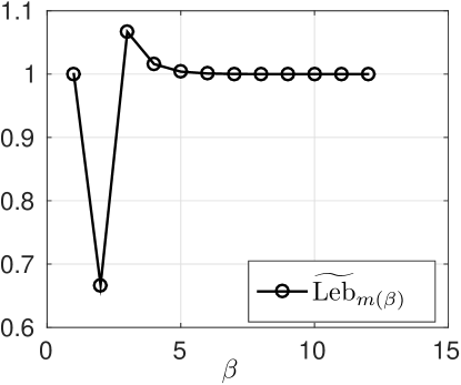
Figure 2: Numerical evaluation of $\widetilde{\textnormal{Leb}}_{m(\beta)}$ for Clenshaw-Curtis points.

Lemma 6 (Stochastic error contribution).

Let $f:\Gamma\to\mathbb{R}$ and ${{{\bm{\beta}}}}\in\mathfrak{L}_{+}$, and assume that the quadrature operator, $\mathscr{Q}^{m({{{\bm{\beta}}}})}$, is built with Clenshaw-Curtis abscissae. If there exists a sequence, ${{\bm{\rho}}}=\{\rho_{j}\}_{j\geq 1}$, $\rho_{j}>1$ for all $j$, such that

1. $\sum_{j\geq 1}\frac{1}{\rho_{j}}<\infty$,

2. there exists $0<C_{f}<\infty$ such that for any finite set, $\mathcal{G}^{\prime}\subset\mathbb{N}_{+}$ with $\#\mathcal{G}^{\prime}<\infty$, the restriction of $f$ on $([-1,1])^{\mathcal{G}^{\prime}}$ admits a holomorphic complex extension in a Bernstein polyellipse, $\mathcal{E}_{{{\bm{\rho}}}}^{\mathcal{G}^{\prime}}$ with $\sup_{{{\bm{z}}}\in\mathcal{E}_{{{\bm{\rho}}}}^{\mathcal{G}^{\prime}}}|f({{\bm{z}}})|\leq C_{f}$.

Then, the set

$$\mathcal{J}=\left\{j\geq 1:\rho_{j}\leq 2(\mathbb{L})^{\frac{1}{3}}\right\},$$

has finite cardinality, i.e., $\#\mathcal{J}<\infty$ and

$$\left|{{\bm{\Delta}}}^{\textnormal{stoc}}[\mathscr{Q}^{m({{{\bm{\beta}}}})}f]\right|\leq C_{\textrm{SE}}({{{\bm{\rho}}}})\sup_{{{\bm{z}}}\in\mathcal{E}_{{{\bm{\rho}}}}^{\mathcal{G}}}|f({{\bm{z}}})|e^{-\sum_{j\geq 1}g_{j}m(\beta_{j}-1)}\leq C_{\textrm{SE}}({{{\bm{\rho}}}})C_{f}e^{-\sum_{j\geq 1}g(\rho_{j})m(\beta_{j}-1)},$$

holds, where $\mathcal{G}$ is the support of ${{{\bm{\beta}}}}-\bm{1}$,

$$0<g(\rho_{j})=\begin{cases}\log\rho_{j},&\text{for }j\in\mathcal{J},\\ \log\rho_{j}-\log 2-\frac{1}{3}\log\left(\mathbb{L}\right),&\text{otherwise},\end{cases}$$

and $C_{\textrm{SE}}({{{\bm{\rho}}}})<\infty$ is independent of ${{{\bm{\beta}}}}$.

Proof.

Let $\mathcal{G}$ be the support of ${{{\bm{\beta}}}}-\bm{1}$ with cardinality $\#\mathcal{G}<\infty$, ${{\bm{k}}}\in\mathbb{N}_{+}^{\mathcal{G}}$, and let $\Phi_{\mathcal{G},{{\bm{k}}}}$ denote the Chebyshev polynomials of the first kind with degree $k_{j}$ along $y_{j}$ for $j\geq 1$. We observe that $\Phi_{\mathcal{G},{{\bm{k}}}}$ are equivalent to the $\#\mathcal{G}$-variate Chebyshev polynomials over $[-1,1]^{\#\mathcal{G}}$ thanks to the product structure of the multivariate Chebyshev polynomials and to the fact that $\phi_{0}(y)=1$. Next, consider the holomorphic extension of $f:\mathbb{C}^{\mathcal{G}}\to\mathbb{C}$, and its Chebyshev expansion over $\Phi_{\mathcal{G},{{\bm{k}}}}$ introduced in Lemma 3, where

$$|{{\bm{\Delta}}}^{\textnormal{stoc}}[\mathscr{Q}^{m({{{\bm{\beta}}}})}f]|=\Big{|}{{\bm{\Delta}}}^{\textnormal{stoc}}\Big{[}\mathscr{Q}^{m({{{\bm{\beta}}}})}\Big{[}\sum_{{{\bm{k}}}\in\mathbb{N}_{+}^{\mathcal{G}}}f_{{\bm{k}}}\Phi_{\mathcal{G},{{\bm{k}}}}\Big{]}\Big{]}\Big{|}=\Big{|}\sum_{{{\bm{k}}}\in\mathbb{N}_{+}^{\mathcal{G}}}f_{{\bm{k}}}{{\bm{\Delta}}}^{\textnormal{stoc}}\Big{[}\mathscr{Q}^{m({{{\bm{\beta}}}})}\big{[}\Phi_{\mathcal{G},{{\bm{k}}}}\big{]}\Big{]}\Big{|}$$

holds. By construction of hierarchical surplus, we have ${{\bm{\Delta}}}^{\textnormal{stoc}}[\mathscr{Q}^{m({{{\bm{\beta}}}})}[\Phi_{\mathcal{G},{{\bm{k}}}}]]=0$ for all Chebyshev polynomials, $\Phi_{\mathcal{G},{{\bm{k}}}}$, such that $\exists\,j\in\mathcal{G}:k_{j}<m(\beta_{j}-1)$ (i.e., for polynomials that are integrated exactly at least in one direction by both quadrature operators along that direction). Therefore, the previous sum reduces to the multi-index set ${{\bm{k}}}\geq m({{{\bm{\beta}}}}-\bm{1})$. Furthermore, by the triangular inequality, we have

$$|{{\bm{\Delta}}}^{\textnormal{stoc}}[\mathscr{Q}^{m({{{\bm{\beta}}}})}f]|\leq\sum_{{{\bm{k}}}\geq m({{{\bm{\beta}}}}-\bm{1})}|f_{{\bm{k}}}|\left|{{\bm{\Delta}}}^{\textnormal{stoc}}\Big{[}\mathscr{Q}^{m({{{\bm{\beta}}}})}\big{[}\Phi_{\mathcal{G},{{\bm{k}}}}\big{]}\Big{]}\right|.$$

Next, using the definitions of ${{\bm{\Delta}}}^{\textnormal{stoc}}$ and $\textnormal{Leb}_{m(\beta)}$ and recalling that Chebyshev polynomials of the first kind on $[-1,1]$ are bounded by $1$, that $\textnormal{Leb}_{m(\beta)}\leq\widetilde{\textnormal{Leb}}_{m(\beta)}\leq 1$ for $\beta=1,2$ and $\textnormal{Leb}_{m(\beta)}\leq\mathbb{L}$ for $\beta\geq 3$, we have

$$\Big{|}{{\bm{\Delta}}}^{\textnormal{stoc}}\Big{[}\mathscr{Q}^{m({{{\bm{\beta}}}})}\big{[}\Phi_{\mathcal{G},{{\bm{k}}}}\big{]}\Big{]}\Big{|} =\left|\bigotimes_{j\in\mathcal{G}}\Delta^{\textnormal{stoc}}_{j}[Q^{m(\beta_{j})}[\phi_{k_{j}}]]\right|$$ (31)

$$\leq\prod_{j\in\mathcal{G}}\widetilde{\textnormal{Leb}}_{m(\beta_{j})}\left\|\phi_{k_{j}}\right\|_{L^{\infty}([-1,1])}\leq\prod_{\beta_{j}\geq 3}\mathbb{L}.$$

We then bound $|f_{{\bm{k}}}|$ by Lemma 3 to obtain

$$|{{\bm{\Delta}}}^{\textnormal{stoc}}[\mathscr{Q}^{m({{{\bm{\beta}}}})}f]| \leq\sup_{{{\bm{z}}}\in\mathcal{E}_{{{\bm{\rho}}}}^{\mathcal{G}}}|f({{\bm{z}}})|\Bigg{(}\prod_{\beta_{j}\geq 3}\mathbb{L}\Bigg{)}\sum_{{{\bm{k}}}\geq m({{{\bm{\beta}}}}-\bm{1})}\prod_{j\in\mathcal{G}}2^{|k_{j}|_{0}}\rho_{j}^{-k_{j}}$$

$$\leq\sup_{{{\bm{z}}}\in\mathcal{E}_{{{\bm{\rho}}}}^{\mathcal{G}}}|f({{\bm{z}}})|\Bigg{(}\prod_{\beta_{j}\geq 3}\mathbb{L}\Bigg{)}\left(\prod_{j\in\mathcal{G}}\sum_{k_{j}\geq m(\beta_{j}-1)}2^{|k_{j}|_{0}}\rho_{j}^{-k_{j}}\right)$$

$$=\sup_{{{\bm{z}}}\in\mathcal{E}_{{{\bm{\rho}}}}^{\mathcal{G}}}|f({{\bm{z}}})|\Bigg{(}\prod_{\begin{subarray}{c}j\in\mathcal{J}\\ \beta_{j}\geq 3\end{subarray}}\mathbb{L}\Bigg{)}\Bigg{(}\prod_{\begin{subarray}{c}j\notin\mathcal{J}\\ \beta_{j}\geq 3\end{subarray}}\mathbb{L}\Bigg{)}$$

$$\hskip 28.45274pt\left(\prod_{j\in\mathcal{G}\cap\mathcal{J}}\sum_{k_{j}\geq m(\beta_{j}-1)}2^{|k_{j}|_{0}}\rho_{j}^{-k_{j}}\right)\left(\prod_{j\in\mathcal{G}\setminus\mathcal{J}}\sum_{k_{j}\geq m(\beta_{j}-1)}2^{|k_{j}|_{0}}\rho_{j}^{-k_{j}}\right).$$

Next, we observe that $|k_{j}|_{0}\leq\min\{1,k_{j}\}$ for $k_{j}\geq 0$ and $1\leq\frac{1}{3}m(\beta_{j}-1)$ for all $\beta_{j}\geq 3$. Then

$$|{{\bm{\Delta}}}^{\textnormal{stoc}}[\mathscr{Q}^{m({{{\bm{\beta}}}})}f]| \leq\sup_{{{\bm{z}}}\in\mathcal{E}_{{{\bm{\rho}}}}^{\mathcal{G}}}|f({{\bm{z}}})|\mathbb{L}^{\#\mathcal{J}}\Bigg{(}\prod_{j\notin\mathcal{J}}\mathbb{L}^{\frac{1}{3}m(\beta_{j}-1)}\Bigg{)}$$

$$\hskip 28.45274pt2^{\#\mathcal{J}}\left(\prod_{j\in\mathcal{G}\cap\mathcal{J}}\sum_{k_{j}\geq m(\beta_{j}-1)}\rho_{j}^{-k_{j}}\right)\left(\prod_{j\in\mathcal{G}\setminus\mathcal{J}}\sum_{k_{j}\geq m(\beta_{j}-1)}2^{k_{j}}\rho_{j}^{-k_{j}}\right)$$

$$\leq\left(2\mathbb{L}\right)^{\#\mathcal{J}}\sup_{{{\bm{z}}}\in\mathcal{E}_{{{\bm{\rho}}}}^{\mathcal{G}}}|f({{\bm{z}}})|\left(\prod_{j\in\mathcal{G}}\sum_{k_{j}\geq m(\beta_{j}-1)}e^{-g(\rho_{j})k_{j}}\right)$$

$$=\left(2\mathbb{L}\right)^{\#\mathcal{J}}\sup_{{{\bm{z}}}\in\mathcal{E}_{{{\bm{\rho}}}}^{\mathcal{G}}}|f({{\bm{z}}})|\left(\prod_{j\in\mathcal{G}}\frac{1}{1-e^{-g(\rho_{j})}}\right)\left(\prod_{j\in\mathcal{G}}e^{-g(\rho_{j})m(\beta_{j}-1)}\right)$$

$$\leq C_{\textrm{SE}}({{{\bm{\rho}}}})\sup_{{{\bm{z}}}\in\mathcal{E}_{{{\bm{\rho}}}}^{\mathcal{G}}}|f({{\bm{z}}})|\prod_{j\geq 1}e^{-g(\rho_{j})m(\beta_{j}-1)},$$

where the last inequality is due to the fact that $m(\beta_{j}-1)=0$ whenever $j\notin\mathcal{G}$ or equivalently $\beta_{j}=1$ and

$$\prod_{j\in\mathcal{G}}\frac{1}{1-e^{-g(\rho_{j})}}\leq\prod_{j>1}\frac{1}{1-e^{-g(\rho_{j})}},$$

since $g(\rho_{j})>0$ for all $j\geq 1$. Note that $C_{\textrm{SE}}({{{\bm{\rho}}}})$ is independent of ${{{\bm{\beta}}}}$ and is bounded since

$$\prod_{j\geq 1}\frac{1}{1-e^{-{g}(\rho_{j})}}<\infty \Longleftrightarrow-\sum_{j\geq 1}\log(1-e^{-{g}(\rho_{j})})<\infty\Longleftrightarrow\sum_{j\geq 1}e^{-{g}(\rho_{j})}<\infty$$

$$\Longleftrightarrow\sum_{j\in\mathcal{J}}\frac{1}{\rho_{j}}+\sum_{j\notin\mathcal{J}}\frac{2\left(\mathbb{L}\right)^{\frac{1}{3}}}{\rho_{j}}<\infty,$$

which was assumed. Moreover, to show that $\#\mathcal{J}<\infty$, note that $\sum_{j\in\mathcal{J}}\rho_{j}^{-1}$ is otherwise unbounded, which contradicts the first assumption of the theorem, namely $\sum_{j\geq 1}\rho_{j}^{-1}<\infty$. ∎

Remark 3.

Sharper estimates could be obtained by exploiting the structure of the Chebyshev polynomials when bounding $\left|{\Delta^{\mathrm{stoc}}[Q^{m(\beta_{j})}[\phi_{k_{j}}]]}\right|$ in (31) (for instance, the fact that $Q^{m(\beta_{j})}[\phi_{k_{j}}]=0$ whenever $k_{j}$ is odd and larger than 1) rather than using the general bound $\Delta^{\mathrm{stoc}}[Q^{m(\beta_{j})}[\phi_{k_{j}}]]\leq\widetilde{\textnormal{Leb}}_{m(\beta_{j})}\left\|\phi_{k_{j}}\right\|_{L^{\infty}([-1,1])}$.

We are now almost in the position to prove the estimate on the error contribution (see Lemma 8); before doing this, we need another auxiliary lemma that gives conditions for the summability of certain sequences that will be considered in the proof of Lemma 8 as well as in the proof of the main theorem on the convergence of MISC.

Lemma 7 (Summability of stochastic rates).

Recall the definitions of $\zeta_{0,j}$ in Lemma 1, of $\zeta_{s,j}$ in Lemma 2 and of $g(\cdot)$ in Lemma 6. Under Assumption A2, for all $s=0,1,\ldots,s_{\max}$, the sequences $\{e^{-g(\zeta_{s,j})}\}_{j\in\mathbb{N}_{+}}$ and $\left\{\frac{1}{\zeta_{s,j}}\right\}_{j\in\mathbb{N}_{+}}$ are $\ell^{p}$-summable for $p\geq\tilde{p}_{s}=\frac{p_{s}}{1-p_{s}}$, with $\tilde{p}_{s}<1$.

Proof.

First note that, by definition of $g(\cdot)$, we have

$$\sum_{j\geq 1}e^{-pg(\zeta_{s,j})}\leq 2^{p}\left(\mathbb{L}\right)^{3p}\sum_{j\geq 1}\zeta_{s,j}^{-p}.$$

Then, from (14)–(15), or (12)–(13) for $s=0$, we can bound $2\tau_{s,j}\leq\zeta_{s,j}$ and obtain

$$\sum_{j\geq 1}\zeta_{s,j}^{-p}\leq 2^{-p}\sum_{j\geq 1}\tau_{s,j}^{-p}=2^{-p}\left(\frac{\pi}{E_{\delta}\left\|{{\bm{b}}}_{s}\right\|_{\ell^{p_{s}}}^{p_{s}}}\right)^{-p}\sum_{j\geq 1}b_{s,j}^{(1-p_{s})p}.$$

From Assumption A2, we know that ${{\bm{b}}}_{s}\in\ell^{p_{s}}$ for $p_{s}\leq\frac{1}{2}$, therefore we have the condition

$$(1-p_{s})p\geq p_{s}\Rightarrow p\geq\frac{p_{s}}{1-p_{s}}<1.$$

∎

Lemma 8 (Total error contribution).

Assume that the deterministic problem is solved with a method obtained by tensorizing piecewise multi-linear finite element spaces on each mesh, $\{\mathbb{T}_{i}\}_{i=1}^{D}$, discretizing each $\{\mathscr{B}_{i}\}_{i=1}^{D}$, and let $h_{i}$ as in (17) be the mesh size of each $\{\mathbb{T}_{i}\}_{i=1}^{D}$. Then, under Assumptions A1 and A2, the error contribution, $\Delta E_{{{{\bm{\alpha}}}},{{{\bm{\beta}}}}}$, of each difference operator, ${{\bm{\Delta}}}[F_{{{{\bm{\alpha}}}},{{{\bm{\beta}}}}}],$ can be decomposed as

$$\Delta E_{{{{\bm{\alpha}}}},{{{\bm{\beta}}}}}\leq\min_{s=0,1,\ldots,s_{\max}}C_{s}\Delta E_{{{{\bm{\alpha}}}}}^{\textnormal{det}}(s)\Delta E_{{{{\bm{\beta}}}}}^{\textnormal{stoc}}(s),$$ (32)

for a constant $C_{s}<\infty$ independent of ${{{\bm{\alpha}}}}$ and ${{{\bm{\beta}}}}$ and

$$\Delta E_{{{{\bm{\alpha}}}}}^{\textnormal{det}}(s) =2^{-{{{\bm{\alpha}}}}\cdot{{\bm{r}}}_{\mathrm{FEM}}(s{{\bm{q}}})},$$ (33)

$$\Delta E_{{{{\bm{\beta}}}}}^{\textnormal{stoc}}(s) =e^{-\sum_{j\geq 1}m(\beta_{j}-1)g_{s,j}},$$ (34)

with $g_{s,j}=g(\zeta_{s,j})$ as in Lemma 6 and $r_{\mathrm{FEM}}(s{{\bm{q}}})_{i}=\min\left\{1,q_{i}s\right\}$ for $i=1,\ldots,D$ with ${{\bm{q}}}\in\mathbb{R}_{+}^{D}$ s.t. $|{{\bm{q}}}|=1$.

Proof.

Combining the definition of ${{\bm{\Delta}}}[F_{{{{\bm{\alpha}}}},{{{\bm{\beta}}}}}]$, cf. (23), and the definition of $\Delta^{\textnormal{det}}[F_{{{{\bm{\alpha}}}},{{{\bm{\beta}}}}}]$, cf. (21), we have

$$\Delta E_{{{{\bm{\alpha}}}},{{{\bm{\beta}}}}}=|{{\bm{\Delta}}}[F_{{{{\bm{\alpha}}}},{{{\bm{\beta}}}}}]| ={{\bm{\Delta}}}^{\textnormal{stoc}}[{{\bm{\Delta}}}^{\textnormal{det}}[F_{{{{\bm{\alpha}}}},{{{\bm{\beta}}}}}]]={{\bm{\Delta}}}^{\textnormal{stoc}}[\sum_{{{\bm{j}}}\in\{0,1\}^{D}}(-1)^{|{{\bm{j}}}|}F_{{{{\bm{\alpha}}}}-{{\bm{j}}},{{{\bm{\beta}}}}}]$$

$$={{\bm{\Delta}}}^{\textnormal{stoc}}[\sum_{{{\bm{j}}}\in\{0,1\}^{D}}(-1)^{|{{\bm{j}}}|}\mathscr{Q}^{m({{{\bm{\beta}}}})}[\Theta[u^{{{{\bm{\alpha}}}}-{{\bm{j}}}}(\cdot,{{\bm{y}}})]]$$

$$={{\bm{\Delta}}}^{\textnormal{stoc}}[\mathscr{Q}^{m({{{\bm{\beta}}}})}\Theta[\sum_{{{\bm{j}}}\in\{0,1\}^{D}}(-1)^{|{{\bm{j}}}|}u^{{{{\bm{\alpha}}}}-{{\bm{j}}}}(\cdot,{{\bm{y}}})]]$$

$$={{\bm{\Delta}}}^{\textnormal{stoc}}[\mathscr{Q}^{m({{{\bm{\beta}}}})}\Theta[{{\bm{\Delta}}}^{\textnormal{det}}[u^{{{{\bm{\alpha}}}}}(\cdot,{{\bm{y}}})]]].$$

We observe that $f({{\bm{y}}})=\Theta[{{\bm{\Delta}}}^{\textnormal{det}}[u^{{{{\bm{\alpha}}}}}(\cdot,{{\bm{y}}})]]$ is a linear combination of some $u^{{{\bm{\alpha}}}}$ and that each of these $u^{{{\bm{\alpha}}}}$ is an $H^{1}_{0}(\mathscr{B},\mathbb{C})$-holomorphic function, since the finite-element approximations of $u$ are holomorphic in the same complex region as $u$ itself; hence, $f({{\bm{y}}})$ is also holomorphic. Then, thanks to the summability properties in Lemma 7, we can apply Lemma 6 in the polyellipses defined in Lemmas 1 and 2 by ${{\bm{\zeta}}}_{s}$ in (14) (or (12) for $s=0$) and obtain

$$\Delta E_{{{{\bm{\alpha}}}},{{{\bm{\beta}}}}} \leq C_{\mathrm{SE}}({{\bm{\zeta}}}_{s})\sup_{{{\bm{z}}}\in\mathcal{E}_{{{\bm{\zeta}}}_{s}}^{\mathcal{G}}}|\Theta[{{\bm{\Delta}}}^{\textnormal{det}}[u^{{{{\bm{\alpha}}}}}({{\bm{x}}},{{\bm{z}}})]|e^{-\sum_{j\geq 1}g(\zeta_{s,j})m(\beta_{j}-1)}$$

$$\leq C_{\mathrm{SE}}({{\bm{\zeta}}}_{s})\left\|\Theta\right\|_{H^{-1}(\mathscr{B})}\sup_{{{\bm{z}}}\in\mathcal{E}_{{{\bm{\zeta}_{s}}}}^{\mathcal{G}}}\left\|{{\bm{\Delta}}}^{\textnormal{det}}[u^{{{{\bm{\alpha}}}}}(\cdot,{{\bm{z}}})]\right\|_{H^{1}(\mathscr{B},\mathbb{C})}e^{-\sum_{j\geq 1}g(\zeta_{s,j})m(\beta_{j}-1)},$$

where $\mathcal{G}\subset\mathbb{N}_{+}$ denotes the support of ${{{\bm{\beta}}}}-\bm{1}$. Next, assuming that the spatial discretization consists of piecewise linear finite elements with spatial mesh sizes (17) and combining the a-priori bounds on the decay of the difference operators coming from the Combination Technique theory (see, e.g., [19, proof of Theorem2]) with (4) and the fact that $u\in H^{1+s}(\mathscr{B})$ for any $s=0,1,\ldots,s_{\max}$, we have the following bound for every ${{\bm{z}}}$ in the Bernstein polyellipse, $\mathcal{E}_{{{\bm{\zeta}}}_{s}}^{\mathcal{G}}$:

$$\left\|{{\bm{\Delta}}}^{\textnormal{det}}[u^{{{{\bm{\alpha}}}}}(\cdot,{{\bm{z}}})]\right\|_{H^{1}(\mathscr{B},\mathbb{C})} \leq C_{CT}\left\|u(\cdot,{{\bm{z}}})\right\|_{\mathcal{H}^{\bm{1}+s{{\bm{q}}}}(\mathscr{B},\mathbb{C})}2^{-\sum_{i=1}^{D}\alpha_{i}\min\{1,q_{i}s\}}$$ (35)

$$\leq C_{CT}C_{s,{{\bm{q}}}}\left\|u(\cdot,{{\bm{z}}})\right\|_{H^{1+s}(\mathscr{B},\mathbb{C})}2^{-{{{\bm{\alpha}}}}\cdot{{\bm{r}}}_{\mathrm{FEM}}(s{{\bm{q}}})},$$ (36)

for ${{\bm{q}}}\in\mathbb{R}_{+}^{D}$ s.t. $q_{i}$ s.t. $|{{\bm{q}}}|=1$, some $C_{CT}>0$ independent of $u$, and where $C_{s,{{\bm{q}}}}$ is the embedding constant between $\mathcal{H}^{\bm{1}+s{{\bm{q}}}}(\mathscr{B},\mathbb{C})$ and $H^{1+s}(\mathscr{B},\mathbb{C})$. We then have the following bound:

$$\Delta E_{{{{\bm{\alpha}}}},{{{\bm{\beta}}}}} \leq C_{\mathrm{SE}}({{\bm{\zeta}}}_{s})\left\|\Theta\right\|_{H^{-1}(\mathscr{B})}C_{CT}C_{s,{{\bm{q}}}}\sup_{{{\bm{z}}}\in\mathcal{E}_{{{\bm{\zeta}}}_{s}}^{\mathcal{G}}}\left\|u(\cdot,{{\bm{z}}})\right\|_{H^{1+s}(\mathscr{B},\mathbb{C})}e^{-\sum_{j}g_{s,j}m(\beta_{j}-1)}2^{-{{{\bm{\alpha}}}}\cdot{{\bm{r}}}_{\mathrm{FEM}}(s{{\bm{q}}})},$$

where the constant, $C_{\mathrm{SE}}({{\bm{\zeta}}}_{s})$ is bounded independently of ${{{\bm{\beta}}}}$, thanks again to Lemma 6. The proof is then concluded by recalling that $\sup_{{{\bm{z}}}\in\mathcal{E}_{{{\bm{\zeta}}}_{s}}^{\mathcal{G}}}\left\|u(\cdot,{{\bm{z}}})\right\|_{H^{1+s}(\mathscr{B},\mathbb{C})}\leq C_{s,u}$ independently of ${{{\bm{\beta}}}}$ and $\mathcal{G}$ due to Lemmas 1 and 2. ∎

Observe that the result in Lemma 8 gives a bound on $\Delta E_{{{{\bm{\alpha}}}},{{{\bm{\beta}}}}}$ parametric on the vector ${{\bm{q}}}$. The optimal choice for such ${{\bm{q}}}$ will be discussed later on, in the proof of the main theorem, namely Theorem 10.

Remark 4 (Relaxing the simplifying assumption).

We now clarify why the assumption $p_{s}<\frac{1}{2}$, for $s=0,1,\ldots,s_{\max}$, is not essential. Due to a suboptimal choice of $\zeta_{s,j}$ in Lemma 2 (and Lemma 1 for $s=0$), the sequence $\{e^{-g_{s,j}}\}_{j\geq 1}$ in Lemma 7, which is related to the solution $u$ and which appears in the proof of the MISC convergence theorem, has worse summability $\tilde{p}_{s}=\frac{p_{s}}{1-p_{s}}$ than the sequence $\{b_{s,j}\}_{j\geq 1}$, whose summability coefficient is $p_{s}$, and which is related to the diffusion coefficient, $a$. As we see in the main theorem stated below, we need $\tilde{p}_{s}<1$ to guarantee convergence of MISC, which implies $p_{s}<\frac{1}{2}$. By choosing the polyellipses in Lemmas 1 and 2 by the more elaborate strategy presented in [11], it would be possible to obtain the better summability $\tilde{p}_{s}=p_{s}$ for the sequence $\{e^{-g_{s,j}}\}_{j\geq 1}$, which would only imply the less stringent condition $p_{s}<1$ and a better estimate for the MISC convergence rate. However, for ease of exposition, we maintain the sub-optimal choice, which is enough for the purpose of presenting the argument that proves convergence of MISC. The restriction $p_{s}<\frac{1}{2}$ formally prevents us from applying the MISC convergence analysis to diffusion coefficients with low spatial regularity. In practice, we see in Section 6 that the convergence estimates are numerically verified beyond this restriction.

Before proving the main theorem of this section, we finally need the following technical lemma.

Lemma 9 (Bounding a sum of double exponentials).

For $a>0$, $b\geq 2$ and $0\leq c<ab$,

$$\sum_{k=1}^{\infty}e^{-ab^{k}+ck}\leq e^{-ab+\varepsilon(a,b,c)}$$

holds, where for each fixed $c$ and $b$, $\varepsilon(\cdot,b,c)$ is a monotonically decreasing, strictly positive function with $\varepsilon(a,b,c)\rightarrow c\mbox{ as }a\rightarrow+\infty$.

Proof.

$$\sum_{k\geq 1}e^{-ab^{k}+ck} =e^{-ab+c}+\sum_{k\geq 2}e^{-ab^{k}+ck}=e^{-ab+c}+\sum_{k\geq 1}e^{-ab^{k+1}+c(k+1)}$$

$$=e^{-ab}\left(e^{c}+e^{c}\sum_{k\geq 1}e^{-ab(b^{k}-1)+ck}\right).$$

We observe that for $b\geq 2$ we have $b^{k}-1\geq k$ for $k\geq 1$ integer. Therefore, $e^{-ab(b^{k}-1)}\leq e^{-abk}$ and we have

$$\sum_{k\geq 1}e^{-ab^{k}+ck}\leq e^{-ab}\left(e^{c}+e^{c}\sum_{k\geq 1}e^{k(c-ab)}\right)=e^{-ab}\left(e^{c}+\frac{e^{2c-ab}}{1-e^{c-ab}}\right).$$

Then,

$$\varepsilon(a,b,c)=\log\left(e^{c}+\frac{e^{2c-ab}}{1-e^{c-ab}}\right),$$

and we finish by verifying that the function, $\varepsilon$, has the required properties. ∎

We are now ready to state and prove our main result.

Theorem 10 (MISC convergence theorem).

Under Assumptions A1—A3, the profit-based MISC estimator, $\mathscr{M}_{\mathcal{I}}$, built using the set $\mathcal{I}$ defined in (29), Stochastic Collocation with Clenshaw-Curtis points as in (19)-(20), and spatial discretization obtained by tensorizing multi-linear piecewise finite element spaces on each mesh, $\{\mathbb{T}_{i}\}_{i=1}^{D}$, with mesh-sizes $h_{i}$ as in (17) for solving the deterministic problems, satisfies, for any $\delta>0$,

$$\big{|}{\mathbb{E}\mspace{-2.0mu}\left[F\right]}-\mathscr{M}_{\mathcal{I}}[F]\big{|}\leq C_{\delta}{\mathrm{Work}\mspace{-2.0mu}\left[\mathscr{M}_{\mathcal{I}}\right]}^{-r_{\mathrm{MISC}}+\delta},$$

for some constant $C_{\delta}>0$ that is independent of ${\mathrm{Work}\mspace{-2.0mu}\left[\mathscr{M}_{\mathcal{I}}\right]}$ and tends to infinity as $\delta\to 0$. Moreover, ${\mathrm{Work}\mspace{-2.0mu}\left[\mathscr{M}_{\mathcal{I}}\right]}$ is given by (27), and

$$r_{\mathrm{MISC}}=\max_{s=0,\ldots,s_{\max}}\begin{cases}r_{\mathrm{det}(s)},&\text{if }r_{\mathrm{det}}(s)\leq\frac{1}{p_{s}}-2,\\ \left(\frac{1}{p_{0}}-2\right)\left(1+\frac{1}{r_{\mathrm{det}}(s)}\left(\frac{1}{p_{0}}-\frac{1}{p_{s}}\right)\right)^{-1},&\text{otherwise,}\end{cases}$$

where

$$r_{\mathrm{det}}(s)=\min\left\{\frac{1}{\max_{i=1,\ldots,D}\gamma_{i}d_{i}},\frac{s}{\sum_{j=1}^{D}\gamma_{j}d_{j}}\right\}.$$

Proof.

In this proof, we use Theorem 4. Therefore, we need to estimate the $p$-summability of the weighted profits for some $p<1$. To this end, we use Lemma 8. Observe that Lemma 8 provides a family of bounds for each $\Delta E_{{{{\bm{\alpha}}}},{{{\bm{\beta}}}}}$, depending on $s$; therefore we would then ideally choose the best $s$ for each $\Delta E_{{{{\bm{\alpha}}}},{{{\bm{\beta}}}}}$. However, this optimization problem is too complex and we simplify it by assuming that

• only two values of $s$ will be considered, $s=0$ and $s=s^{*}$ (which will not necessarily coincide with $s_{\max}$);

• the optimization between $s=0$ and $s=s^{*}$ will not be carried out individually on each $\Delta E_{{{{\bm{\alpha}}}},{{{\bm{\beta}}}}}$, but we will rather take a “convex combination” of the two corresponding estimates and choose the best outcome only at the end of the proof.

To this end, we first need to rewrite the result of the Lemma 8 in a more suitable form for any fixed $s^{*}\in\{1,2,\ldots,s_{\max}\}$; note that from here on, with a slight abuse of notation, we drop the superscript ^∗ and simply use $s$ to denote the fixed value. Thus, for such fixed $s$, consider the statement of Lemma 8, let $C_{E}=\max\{C_{0},C_{s}\}$, $\chi_{j,s}=g_{s,j}\log_{2}e$, and $\theta_{j,s}=(g_{0,j}-g_{s,j})\log_{2}e$ and combine (32)–(34), obtaining

$$\Delta E_{{{{\bm{\alpha}}}},{{{\bm{\beta}}}}} \leq\min_{t=\{0,s\}}C_{t}\Delta E_{{{{\bm{\alpha}}}}}^{\textnormal{det}}(t)\Delta E_{{{{\bm{\beta}}}}}^{\textnormal{stoc}}(t)\leq C_{E}\min_{\eta\in\{0,1\}}2^{-\eta{{\bm{r}}}_{\mathrm{FEM}}(s{{\bm{q}}})\cdot{{{\bm{\alpha}}}}}\prod_{j\geq 1}e^{-m(\beta_{j}-1)[g_{s,j}+(1-\eta)(g_{0,j}-g_{s,j})]}$$

$$=C_{E}\min_{\eta\in\{0,1\}}2^{-\eta{{\bm{r}}}_{\mathrm{FEM}}(s{{\bm{q}}})\cdot{{{\bm{\alpha}}}}}\prod_{j\geq 1}2^{-m(\beta_{j}-1)[g_{s,j}+(1-\eta)(g_{0,j}-g_{s,j})]\log_{2}e}$$

$$=C_{E}\min_{\eta\in\{0,1\}}2^{-\eta{{\bm{r}}}_{\mathrm{FEM}}(s{{\bm{q}}})\cdot{{{\bm{\alpha}}}}}\prod_{j\geq 1}2^{-m(\beta_{j}-1)[\chi_{j,s}+(1-\eta)\theta_{j,s}]}$$

$$=C_{E}2^{-\sum_{j\geq 1}m(\beta_{j}-1)\chi_{j,s}-\max_{\eta\in\{0,1\}}\left(\eta{{\bm{r}}}_{\mathrm{FEM}}(s{{\bm{q}}})\cdot{{{\bm{\alpha}}}}+\sum_{j\geq 1}m(\beta_{j}-1)(1-\eta)\theta_{j,s}\right)}$$

$$=C_{E}2^{-\sum_{j\geq 1}m(\beta_{j}-1)\chi_{j,s}-\max\left\{\sum_{j\geq 1}m(\beta_{j}-1)\theta_{j,s},\,\,{{\bm{r}}}_{\mathrm{FEM}}(s{{\bm{q}}})\cdot{{{\bm{\alpha}}}}\right\}}.$$

for an arbitrary ${{\bm{q}}}\in\mathbb{R}_{+}^{D}$ with $|{{\bm{q}}}|=1$ that we will choose later. We can now bound the weighted sum of the profits as follows:

$$\sum_{[{{{\bm{\alpha}}}},{{{\bm{\beta}}}}]\in\mathbb{N}_{+}^{D}\times\mathfrak{L}_{+}}P_{{{{\bm{\alpha}}}},{{{\bm{\beta}}}}}^{p}\Delta W_{{{{\bm{\alpha}}}},{{{\bm{\beta}}}}}=\sum_{[{{{\bm{\alpha}}}},{{{\bm{\beta}}}}]\in\mathbb{N}_{+}^{D}\times\mathfrak{L}_{+}}\Delta E_{{{{\bm{\alpha}}}},{{{\bm{\beta}}}}}^{p}\Delta W_{{{{\bm{\alpha}}}}}^{1-p}\Delta W_{{{{\bm{\beta}}}}}^{1-p}$$

$$\leq C_{E}^{p}C_{W}^{1-p}\sum_{[{{{\bm{\alpha}}}},{{{\bm{\beta}}}}]\in\mathbb{N}_{+}^{D}\times\mathfrak{L}_{+}}2^{-p[\max\{{{\bm{r}}}_{\mathrm{FEM}}(s{{\bm{q}}})\cdot{{{\bm{\alpha}}}},\sum_{j\geq 1}m(\beta_{j}-1)\theta_{s,j}\}+\sum_{j\geq 1}m(\beta_{j}-1)\chi_{s,j}]}$$

$$\hskip 113.81102pt\cdot 2^{(1-p)\sum_{i=1}^{D}\gamma_{i}d_{i}\alpha_{i}+(1-p)\sum_{j\geq 1}(\beta_{j}-1)}$$

$$=C_{E}^{p}C_{W}^{1-p}\sum_{[{{{\bm{\alpha}}}},{{{\bm{\beta}}}}]\in\mathbb{N}_{+}^{D}\times\mathfrak{L}_{+}}\min_{\lambda\in[0,1]}2^{-p[\lambda{{\bm{r}}}_{\mathrm{FEM}}(s{{\bm{q}}})\cdot{{{\bm{\alpha}}}}+(1-\lambda)\sum_{j\geq 1}m(\beta_{j}-1)\theta_{s,j}+\sum_{j\geq 1}m(\beta_{j}-1)\chi_{s,j}]}$$

$$\hskip 142.26378pt\cdot 2^{(1-p)\sum_{i=1}^{D}\gamma_{i}d_{i}\alpha_{i}+(1-p)\sum_{j\geq 1}(\beta_{j}-1)}$$

$$\leq C_{E}^{p}C_{W}^{1-p}\min_{\lambda\in[0,1]}\sum_{[{{{\bm{\alpha}}}},{{{\bm{\beta}}}}]\in\mathbb{N}_{+}^{D}\times\mathfrak{L}_{+}}2^{-p[\lambda{{\bm{r}}}_{\mathrm{FEM}}(s{{\bm{q}}})\cdot{{{\bm{\alpha}}}}+(1-\lambda)\sum_{j\geq 1}m(\beta_{j}-1)\theta_{s,j}+\sum_{j\geq 1}m(\beta_{j}-1)\chi_{s,j}]}$$

$$\hskip 142.26378pt\cdot 2^{(1-p)\sum_{i=1}^{D}\gamma_{i}d_{i}\alpha_{i}+(1-p)\sum_{j\geq 1}(\beta_{j}-1)}$$

$$=C_{E}^{p}C_{W}^{1-p}\min_{\lambda\in[0,1]}\left(\prod_{i=1}^{D}\sum_{k=1}^{\infty}2^{-[p(\lambda r_{\mathrm{FEM}}(s{{\bm{q}}})_{i}+\gamma_{i}d_{i})-\gamma_{i}d_{i}]k}\right)$$

$$\hskip 85.35826pt\cdot\left(\prod_{j=1}^{\infty}\sum_{k=1}^{\infty}2^{-pm(k-1)((1-\lambda)\theta_{s,j}+\chi_{s,j})+(1-p)(k-1)}\right).$$ (37)

We then investigate under what conditions each of the two factors is finite (the constants $C_{E},C_{W}$ are bounded, cf. Lemmas 5 and 8). Before proceeding, we comment on the equations above. As we already mentioned at the beginning of the proof, here we are working in a suboptimal setting in which instead of choosing a different $s$ for each $\Delta E_{{{{\bm{\alpha}}}},{{{\bm{\beta}}}}}$, we restrict ourselves to choosing between only two values, $s=0$ or a certain $s>0$ (second line). Observe that we have an equality between the second and the third line since $2^{x}$ is a monotone function of $x$. Hence, the minimum is always attained at either $\lambda=0$ or $\lambda=1$. However, when it comes to switching the order of the sum and the minimum in the fourth line, i.e., bounding the sum by choosing the same $\lambda$ to bound every term in the sum, allowing for fractional $\lambda$ gives a tighter bound on the overall sum than just considering $\lambda\in\{0,1\}$. Roughly speaking, we are somehow “mimicking” the fact that the optimal bound of the sum would use a different value of $\lambda$ for every term by choosing an overall $\lambda$ that is between the two possible values.

To investigate the condition for which each of the two factors in (37) are bounded, we immediately have for the first factor for all $i=1,\ldots,D$ that

$${p\left(\lambda r_{\mathrm{FEM}}(s{{\bm{q}}})_{i}+\gamma_{i}d_{i}\right)-\gamma_{i}d_{i}}>0\quad\Longrightarrow\quad p>\frac{\gamma_{i}d_{i}}{\lambda r_{\mathrm{FEM}}(s{{\bm{q}}})_{i}+\gamma_{i}d_{i}}=\left(\lambda\frac{r_{\mathrm{FEM}}(s{{\bm{q}}})_{i}}{\gamma_{i}d_{i}}+1\right)^{-1}\,\,.$$ (38)

Our goal is to optimize the above constraint for the summability exponent $p$. To this end, we will minimize the right hand side of (38), observing that it decreases with respect to $r_{\mathrm{FEM}}(s{{\bm{q}}})_{i}$. Hence, recalling the dependence of $r_{\mathrm{FEM}}(s{{\bm{q}}})_{i}$ (cf. Lemma 8) on the vector of weights ${{\bm{q}}}$ we consider

$$r_{\mathrm{det}}(s) =\max_{{{\bm{q}}}\in\mathbb{R}^{D}_{+},|{{\bm{q}}}|=1}\min_{i=1,\ldots,D}\frac{r_{\mathrm{FEM}}(s{{\bm{q}}})_{i}}{\gamma_{i}d_{i}}$$

$$=\max_{{{\bm{q}}}\in\mathbb{R}^{D}_{+},|{{\bm{q}}}|=1}\min_{i=1,\ldots,D}\min\left\{\frac{1}{\gamma_{i}d_{i}},\frac{sq_{i}}{\gamma_{i}d_{i}}\right\}$$

$$=\max_{{{\bm{q}}}\in\mathbb{R}^{D}_{+},|{{\bm{q}}}|=1}\min\left(\frac{1}{\max_{i=1,\ldots,D}\gamma_{i}d_{i}},\min_{i=1,\ldots,D}\frac{sq_{i}}{\gamma_{i}d_{i}}\right)$$

$$=\min\left(\frac{1}{\max_{i=1,\ldots,D}\gamma_{i}d_{i}},\max_{{{\bm{q}}}\in\mathbb{R}^{D}_{+},|{{\bm{q}}}|=1}\min_{i=1,\ldots,D}\frac{sq_{i}}{\gamma_{i}d_{i}}\right)$$

which is maximized by making $\frac{sq_{i}}{\gamma_{i}d_{i}}$ constant over $i$, i.e.

$$q_{i}=\frac{\gamma_{i}d_{i}}{\sum_{j=1}^{D}\gamma_{j}d_{j}}\Rightarrow r_{\mathrm{det}}(s)=\min\left\{\frac{1}{\max_{i=1,\ldots,D}\gamma_{i}d_{i}},\frac{s}{\sum_{j=1}^{D}\gamma_{j}d_{j}}\right\}.$$

With this optimal choice then (38) becomes simply

$$p>\left(\lambda r_{\mathrm{det}}(s)+1\right)^{-1}\,\,.$$ (39)

For the second factor, denoting the generic term of the inner sum as $a_{j,k}$ for brevity and observing that $a_{j,1}=1$ for every $j$, we have

$$\prod_{j=1}^{\infty}\sum_{k=1}^{\infty}a_{j,k} \leq\prod_{j=1}^{\infty}\left(1+\sum_{k=2}^{\infty}a_{j,k}\right)=\exp\left(\sum_{j=1}^{\infty}\log\left(1+\sum_{k=2}^{\infty}a_{j,k}\right)\right)\leq\exp\left(\sum_{j=1}^{\infty}\sum_{k=2}^{\infty}a_{j,k}\right).$$

We thus only have to discuss the convergence of the sum

$$\sum_{j=1}^{\infty}\sum_{k=2}^{\infty}2^{-pm(k-1)[(1-\lambda)\theta_{s,j}+\chi_{s,j}]+(1-p)(k-1)} =\sum_{j=1}^{\infty}\sum_{k=1}^{\infty}2^{-pm(k)[(1-\lambda)\theta_{s,j}+\chi_{s,j}]+(1-p)k}$$ (40)

$$\leq\sum_{j=1}^{\infty}\sum_{k=1}^{\infty}2^{-p2^{k-1}[(1-\lambda)\theta_{s,j}+\chi_{s,j}]+(1-p)k}\,,$$

where the last step is a consequence of the fact that, for Clenshaw-Curtis points, $m(k)\geq 2^{k-1}$ for $k\geq 1$, cf. (20). Moreover, $(1-\lambda)\theta_{s,j}+\chi_{s,j}\geq 0$. To study the summability of (40), we want to use Lemma 9 to bound the inner sum in (40). First, we rewrite

$$\sum_{k=1}^{\infty}2^{-p2^{k-1}[(1-\lambda)\theta_{s,j}+\chi_{s,j}]+(1-p)k} =\sum_{k=1}^{\infty}\exp\left(-p\frac{\log 2}{2}[(1-\lambda)\theta_{s,j}+\chi_{s,j}]2^{k}+(1-p)k\log 2\right)$$

$$=\sum_{k=1}^{\infty}\exp\left(-a2^{k}+ck\right)$$

$$\mbox{ with }a=p\frac{\log 2}{2}[(1-\lambda)\theta_{s,j}+\chi_{s,j}]>0,\quad c=(1-p)\log 2>0,$$

where we have used the notation in Lemma 9. Note that this lemma holds true under the assumptions that $a>0$ and $0\leq c<2a$, where the latter has to be verified as follows

$$2a>c\Leftrightarrow p\log 2[(1-\lambda)\theta_{s,j}+\chi_{s,j}]>(1-p)\log 2\Leftrightarrow(1-\lambda)\theta_{s,j}+\chi_{s,j}>\frac{(1-p)}{p},$$

which is true whenever

$$\chi_{s,j}>r_{\text{det}}(s),$$

due to (39), $\theta_{s,j}\geq 0$ and $\lambda\leq 1$. Define $\overline{\mathcal{J}}=\{j\geq 1\>:\>\chi_{s,j}\leq r_{\text{det}}(s)\}$ which has a finite cardinality since $\chi_{s,j}\to\infty$ as $j\to\infty$. Resuming from (40), we have, due to Lemma 9,

$$\sum_{j=1}^{\infty}\sum_{k=1}^{\infty}2^{-p2^{k-1}[(1-\lambda)\theta_{s,j}+\chi_{s,j}]+(1-p)k} \leq C(\overline{\mathcal{J}})+\sum_{j\notin\overline{\mathcal{J}}}\sum_{k=1}^{\infty}\exp\left(-a2^{k}+ck\right)$$

$$\leq C(\overline{\mathcal{J}})+\sum_{j\notin\overline{\mathcal{J}}}e^{-2a+\varepsilon(a,2,c)},$$

where $C(\overline{\mathcal{J}})$ is bounded, since $\#\overline{\mathcal{J}}<\infty$, and $\varepsilon(a,2,c)$ is a monotonically decreasing function with limit $c=(1-p)\log 2$ independent of $j$. Therefore, the previous series converges if and only if

$$\sum_{j\notin\overline{\mathcal{J}}}^{\infty}e^{-2a}=\sum_{j\notin\overline{\mathcal{J}}}^{\infty}e^{-p\log 2[(1-\lambda)\theta_{s,j}+\chi_{s,j}]}=\sum_{j\notin\overline{\mathcal{J}}}^{\infty}2^{-p[(1-\lambda)\theta_{s,j}+\chi_{s,j}]}$$

converges. Inserting the expression of $\theta_{s,j}$ and $\chi_{s,j}$, we get

$$\sum_{j\notin\overline{\mathcal{J}}}^{\infty}2^{-p[(1-\lambda)\theta_{s,j}+\chi_{s,j}]} =\sum_{j\notin\overline{\mathcal{J}}}^{\infty}2^{-p[(1-\lambda)(g_{0,j}-g_{s,j})+g_{s,j}]\log_{2}e}=\sum_{j\notin\overline{\mathcal{J}}}^{\infty}e^{-p[(1-\lambda)(g_{0,j}-g_{s,j})+g_{s,j}]}$$

$$=\sum_{j\notin\overline{\mathcal{J}}}^{\infty}e^{-p(1-\lambda)g_{0,j}}e^{-p\lambda g_{s,j}}.$$

After applying the Hölder inequality in the previous summation with exponents $\eta_{1}^{-1}+\eta_{2}^{-1}=1$ we need to simultaneously ensure the boundedness of the following sums:

$$\sum_{j\notin\overline{\mathcal{J}}}^{\infty}e^{-p(1-\lambda)g_{0,j}\eta_{2}}\quad\text{and}\quad\sum_{j\notin\overline{\mathcal{J}}}^{\infty}e^{-p\lambda g_{s,j}\eta_{1}}.$$

Recalling the summability result in Lemma 7, we understand that the following two conditions must hold:

$$\begin{cases}\displaystyle p(1-\lambda)\eta_{2}\geq\frac{p_{0}}{1-p_{0}}\\[10.0pt] \displaystyle p\lambda\eta_{1}\geq\frac{p_{s}}{1-p_{s}}\end{cases}\Rightarrow\begin{cases}\displaystyle p\geq\frac{p_{0}}{1-p_{0}}\frac{1}{1-\lambda}\frac{1}{\eta_{2}}\\[10.0pt] \displaystyle p\geq\frac{p_{s}}{1-p_{s}}\frac{1}{\lambda}\left(1-\frac{1}{\eta_{2}}\right),\end{cases}$$

which closes the discussion of the summability of the second factor of (37) for a fixed $s$. Recalling the constraint (39) coming from the first factor of (37), we finally have to solve the following optimization problem:

$$p>\min_{\lambda\in[0,1],1\leq\eta_{2}}\max\left\{\left(\lambda r_{\mathrm{det}}(s)+1\right)^{-1},\frac{p_{s}}{1-p_{s}}\frac{1}{\lambda}\left(1-\frac{1}{\eta_{2}}\right),\frac{p_{0}}{1-p_{0}}\frac{1}{1-\lambda}\frac{1}{\eta_{2}}\right\}$$

i.e., we have to choose $\eta_{2}$ and $\lambda$ to minimize the lower bound on $p$. We first optimally select $\eta_{2}$ given $\lambda$, i.e., we take $\eta_{2}=\eta_{2}^{*}$ such that

$$\frac{p_{s}}{1-p_{s}}\frac{1}{\lambda}\left(1-\frac{1}{\eta_{2}^{*}}\right)=\frac{p_{0}}{1-p_{0}}\frac{1}{1-\lambda}\frac{1}{\eta_{2}^{*}}\,\,\Rightarrow\,\,\eta_{2}^{*}=1+\frac{1-p_{s}}{p_{s}}\frac{p_{0}}{1-p_{0}}\frac{\lambda}{1-\lambda}$$

Substituting back, we obtain

$$\frac{p_{s}}{1-p_{s}}\frac{1}{\lambda}\frac{\eta_{2}^{*}-1}{\eta_{2}^{*}} =\left({\frac{1}{p_{0}}-1+\lambda\left(\frac{1}{p_{s}}-\frac{1}{p_{0}}\right)}\right)^{-1},$$

so that the minimization problem reads

$$p >\min_{\lambda\in[0,1]}\max\left\{f_{1}(\lambda,s),f_{2}(\lambda,s)\right\},$$ (41)

$$f_{1}(\lambda,s)=\left(\lambda r_{\mathrm{det}}(s)+1\right)^{-1},\quad f_{2}(\lambda,s)=\left({\frac{1}{p_{0}}-1+\lambda\left(\frac{1}{p_{s}}-\frac{1}{p_{0}}\right)}\right)^{-1}.$$

Now, we recall that $p_{0}\leq p_{s}$. Hence, $f_{2}(\lambda,s)$ is increasing with $\lambda$. Conversely, $f_{1}(\lambda,s)$ is decreasing with $\lambda$ since $r_{\mathrm{det}}(s)$ is a positive number. Furthermore, notice that we cannot have $f_{1}(\lambda,s)<f_{2}(\lambda,s)$ for all $\lambda\in[0,1]$. Indeed, the previous condition is equivalent to $f_{1}(0,s)\leq f_{2}(0,s)$, i.e., $1\leq\frac{p_{0}}{1-p_{0}}\Rightarrow p_{0}\geq\frac{1}{2}$, which does not satisfy Assumption A2. Note that, in this case, the lower bound for $p$ in (41) is minimized for $\lambda=0$, implying that $p>\frac{p_{0}}{1-p_{0}}>1$, i.e., the method does not converge (cf. the statement of Theorem 4). Thus, we have only two cases (see also Figure 3):

Case 1

$f_{1}(\lambda,s)>f_{2}(\lambda,s)$ for all $\lambda\in[0,1]$, which means that the convergence of the method is dictated by the spatial discretization. Given that $f_{1}$ is decreasing and $f_{2}$ is increasing, the previous condition is equivalent to $f_{1}(1,s)\geq f_{2}(1,s)$, i.e., $r_{\mathrm{det}}(s)\leq\frac{1}{p_{s}}-2$. In this case, the lower bound (41) is minimized for $\lambda=1$, and we have $p>\left(r_{\mathrm{det}}(s)+1\right)^{-1}$.

Case 2

There exists $\lambda^{*}\in(0,1)$ such that $f_{1}(\lambda,s)=f_{2}(\lambda,s)$. This condition is equivalent to the two conditions

$$\begin{cases}f_{1}(0,s)\geq f_{2}(0,s)\\ f_{1}(1,s)\leq f_{2}(1,s)\end{cases}\Rightarrow\begin{cases}1\leq\frac{1}{p_{0}}-1\\ r_{\mathrm{det}}(s)\geq\frac{1}{p_{s}}-2.\end{cases}$$

Solving for $\lambda^{*}$ yields

$$\lambda^{*} =\frac{\frac{1}{p_{0}}-2}{r_{\mathrm{det}}(s)+\frac{1}{p_{0}}-\frac{1}{p_{s}}}>0$$

which yields $p>\overline{p}$, where

$$\overline{p} =\left(\left(\frac{\frac{1}{p_{0}}-2}{r_{\mathrm{det}}(s)+\frac{1}{p_{0}}-\frac{1}{p_{s}}}\right)r_{\mathrm{det}}(s)+1\right)^{-1}$$

$$=\left(1+\left(\frac{1}{p_{0}}-2\right)\left(1+\frac{1}{r_{\mathrm{det}}(s)}\left(\frac{1}{p_{0}}-\frac{1}{p_{s}}\right)\right)^{-1}\right)^{-1}\,\,.$$

Since the previous computations were carried out for a fixed $s$, we can take the minimum over all possible values of $s$. Then, we can apply Theorem 4 and derive the convergence estimate,

$$\big{|}{\mathbb{E}\mspace{-2.0mu}\left[F\right]}-\mathscr{M}_{\mathcal{I}}[F]\big{|}\leq C_{P}(p){\mathrm{Work}\mspace{-2.0mu}\left[\mathscr{M}_{\mathcal{I}}\right]}^{1-1/p},$$

where $1-1/p=1-\max_{s=0,\ldots,s_{\max}}(1/{\overline{p}})+\delta$ for any $\delta>0$, which we reformulate as

$$\big{|}{\mathbb{E}\mspace{-2.0mu}\left[F\right]}-\mathscr{M}_{\mathcal{I}}[F]\big{|}\leq C_{P}\left(\frac{1}{1+r_{\mathrm{MISC}}-\delta}\right){\mathrm{Work}\mspace{-2.0mu}\left[\mathscr{M}_{\mathcal{I}}\right]}^{-r_{\mathrm{MISC}}+\delta},$$

with $r_{\mathrm{MISC}}=\max_{s=0,\ldots,s_{\max}}({1}/{\overline{p}})-1$. ∎

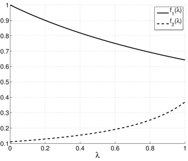
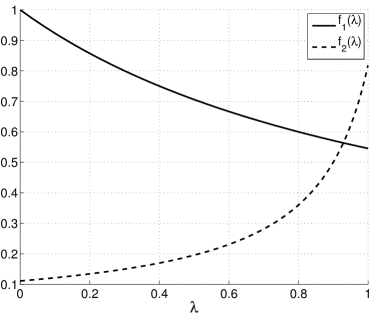
Figure 3: Illustration of the optimization problem (41). As observed in the proof, $f_{1}$ is decreasing with $\lambda$ while $f_{2}$ is increasing with $\lambda$. Left: case 1 of the proof: the minmax point is $\lambda=1$; Right: case 2 of the proof: the minmax point is $\lambda<1$.

5 Analysis of Example 1

In this section, we determine the value of $s_{\max}$ and the sequence $\{p_{s}\}_{s=0}^{s_{\max}}$ for Example 1. Since we will work with localized quantities of interest far from the boundary, cf. equation (45) written below, we believe that the effect of the boundary is negligible and the regularity $s_{\max}$ is mainly limited by the summability properties of $\kappa$. See Appendix B for a slightly modified problem on the same domain where we can prove that the regularity is only limited by the summability properties of $\kappa$. Let us define the following family of auxiliary functions,

$$\Upsilon_{{{\bm{k}}},{{\bm{\ell}}}}({{\bm{x}}})=\prod_{i=1}^{d}\left(\cos\left({\pi}k_{i}x_{i}\right)\right)^{\ell_{i}}\left(\sin\left({\pi}k_{i}x_{i}\right)\right)^{1-\ell_{i}},$$

so that $\kappa$ from (8) can be written as

$$\kappa({{\bm{x}}},{{\bm{y}}}) =\sum_{{{\bm{k}}}\in\mathbb{N}^{d}}A_{{{\bm{k}}}}\sum_{{{\bm{\ell}}}\in\{0,1\}^{d}}y_{{{\bm{k}}},{{\bm{\ell}}}}\Upsilon_{{{\bm{k}}},{{\bm{\ell}}}}({{\bm{x}}})$$

$$=\sum_{j=0}^{\infty}\sum_{\left\{{{\bm{k}}}\in\mathbb{N}^{d}\>:\>|{{\bm{k}}}|=j\right\}}A_{{{\bm{k}}}}\sum_{{{\bm{\ell}}}\in\{0,1\}^{d}}y_{{{\bm{k}}},{{\bm{\ell}}}}\Upsilon_{{{\bm{k}}},{{\bm{\ell}}}}({{\bm{x}}}).$$

Based on this expression, for $s\geq 0$, we analyze the summability of $\left\{A_{{{\bm{k}}}}\|D^{{{\bm{s}}}}\Upsilon_{{{\bm{k}}},{{\bm{\ell}}}}\|_{L^{\infty}(\mathscr{B})}\right\}$ for $|{{\bm{s}}}|=s$ to determine the permissible values of $p_{s}$. First, for $|{{\bm{s}}}|=s$, observe that for a constant $c$ independent of ${{\bm{k}}}$ we have

$$\|D^{{{\bm{s}}}}\Upsilon_{{{\bm{k}}},{{\bm{\ell}}}}({{\bm{x}}})\|_{L^{\infty}(\mathscr{B})}=\prod_{j=1}^{d}\left({\pi}k_{j}\right)^{s_{j}}\leq c|{{\bm{k}}}|^{s}.$$

Then for all $s\geq 0$, we have

$$\sum_{j=0}^{\infty}\sum_{\left\{{{\bm{k}}}\in\mathbb{N}^{d}\>:\>|{{\bm{k}}}|=j\right\}}\sum_{{{\bm{\ell}}}\in\{0,1\}^{d}}A_{{{\bm{k}}}}^{p_{s}}\|D^{{{\bm{s}}}}\Upsilon_{{{\bm{k}}},{{\bm{\ell}}}}\|_{L^{\infty}(\mathscr{B})}^{p_{s}} \leq c2^{d}\sum_{j=0}^{\infty}\sum_{\left\{{{\bm{k}}}\in\mathbb{N}^{d}\>:\>|{{\bm{k}}}|=j\right\}}2^{p_{s}{\frac{|{{\bm{k}}}|_{0}}{2}}}|{{\bm{k}}}|^{p_{s}s}(1+|{{\bm{k}}}|^{2})^{-\frac{p_{s}\left(\nu+\frac{d}{2}\right)}{2}}$$

$$\leq c2^{d}+c2^{d+p_{s}\frac{d}{2}}\sum_{j=1}^{\infty}\sum_{\left\{{{\bm{k}}}\in\mathbb{N}^{d}\>:\>|{{\bm{k}}}|=j\right\}}j^{-p_{s}\left(\nu+\frac{d}{2}-s\right)}$$

$$=c2^{d}+c\frac{2^{d+p_{s}\frac{d}{2}}}{(d-1)!}\sum_{j=1}^{\infty}j^{-p_{s}\left(\nu+\frac{d}{2}-s\right)}\prod_{i=1}^{d-1}(j+i)$$

$$=c2^{d}+c\frac{2^{d+p_{s}\frac{d}{2}}}{(d-1)!}\sum_{j=1}^{\infty}j^{-p_{s}\left(\nu+\frac{d}{2}-s\right)+d-1}\left(1+\frac{d-1}{j}\right)^{d-1}$$

$$\leq c2^{d}+\frac{c2^{d+p_{s}\frac{d}{2}}d^{d-1}}{(d-1)!}\sum_{j=1}^{\infty}j^{-p_{s}\left(\nu+\frac{d}{2}-s\right)+d-1}.$$

From here, we obtain the bound

$$p_{s}>\left(\frac{\nu}{d}+\frac{1}{2}-\frac{s}{d}\right)^{-1},$$ (42)

for all $s\geq 0$. Moreover, imposing $p_{0}<\frac{1}{2}$ and $p_{s_{\max}}<\frac{1}{2}$ gives the bounds

$$\nu>\frac{3d}{2}\qquad\text{ and }\ \qquad s_{\max}<\nu-\frac{3d}{2},$$ (43)

respectively. Since $\Upsilon_{{{\bm{k}}},{{\bm{\ell}}}}\in C^{\infty}(\mathscr{B})$, the bounds in (43) are the only bounds on the value of $s_{\max}$. To determine an upper bound on the value of $r_{\text{MISC}}$, up to a small $\delta$, we set $\gamma_{1}=\ldots=\gamma_{D}=\gamma$ (motivated by the fact that all subdomains $\mathscr{B}_{i}$ are equal), we substitute $r_{\text{FEM},i}(s)=\min(1,\frac{s}{d})$ for $i=1,\ldots,d$ and the lower bound of $p_{s}$ in Theorem 10 and obtain after simplifying

$$r_{\mathrm{MISC}} =\max_{s=0,\ldots,s_{\max}}\begin{cases}\frac{\min(1,\frac{s}{d})}{\gamma}&\text{ if }\frac{\min(1,\frac{s}{d})}{\gamma}\leq\frac{\nu}{d}-\frac{3}{2}-\frac{s}{d},\\ \left(\frac{\nu}{d}-\frac{3}{2}\right)\left(1+\frac{\gamma}{\min(1,\frac{s}{d})}\frac{s}{d}\right)^{-1}&\text{ if }\frac{\min(1,\frac{s}{d})}{\gamma}\geq\frac{\nu}{d}-\frac{3}{2}-\frac{s}{d},\end{cases}$$

$$=\max_{s=0,\ldots,s_{\max}}\begin{cases}\frac{s}{d\gamma}&\text{ if }\frac{s}{d\gamma}\leq\frac{\nu}{d}-\frac{3}{2}-\frac{s}{d}\text{ and }s\leq d,\\ \left(\frac{\nu}{d}-\frac{3}{2}\right)\left(1+\gamma\right)^{-1}&\text{ if }\frac{s}{d\gamma}\geq\frac{\nu}{d}-\frac{3}{2}-\frac{s}{d}\text{ and }s\leq d,\\ \frac{1}{\gamma}&\text{ if }\frac{1}{\gamma}\leq\frac{\nu}{d}-\frac{3}{2}-\frac{s}{d}\text{ and }s\geq d,\\ \left(\frac{\nu}{d}-\frac{3}{2}\right)\left(1+\frac{s\gamma}{d}\right)^{-1}&\text{ if }\frac{1}{\gamma}\geq\frac{\nu}{d}-\frac{3}{2}-\frac{s}{d}\text{ and }s\geq d.\end{cases}$$

Before continuing, we discuss the four branches of the previous expression. If $s_{\max}\leq d$, then only the first two branches are valid. Since the rates in these two branches increase with $s$, the maximum is achieved for $s=s_{\max}$. If $s_{\max}\geq d$, then, since the rates in the third and fourth branches decrease with $s$, the maximum is achieved for $s=d$. Hence

$$r_{\mathrm{MISC}} =\begin{cases}\frac{s_{\max}}{d\gamma}&\text{ if }\frac{s_{\max}(1+\gamma)}{d\gamma}\leq\frac{\nu}{d}-\frac{3}{2}\text{ and }s_{\max}\leq d,\\ \left(\frac{\nu}{d}-\frac{3}{2}\right)\left(1+\gamma\right)^{-1}&\text{ if }\frac{s_{\max}(1+\gamma)}{d\gamma}\geq\frac{\nu}{d}-\frac{3}{2}\text{ and }s_{\max}\leq d,\\ \frac{1}{\gamma}&\text{ if }\frac{1}{\gamma}\leq\frac{\nu}{d}-\frac{3}{2}-1\text{ and }s_{\max}\geq d,\\ \left(\frac{\nu}{d}-\frac{3}{2}\right)\left(1+\gamma\right)^{-1}&\text{ if }\frac{1}{\gamma}\geq\frac{\nu}{d}-\frac{3}{2}-1\text{ and }s_{\max}\geq d,\end{cases}$$

$$=\begin{cases}\frac{1}{\gamma}\left(\frac{\nu}{d}-\frac{3}{2}\right)&\text{ if }\frac{1}{\gamma}\leq 0\text{ and }\frac{\nu}{d}\leq\frac{5}{2},\\ \left(\frac{\nu}{d}-\frac{3}{2}\right)\left(1+\gamma\right)^{-1}&\text{ if }\frac{1}{\gamma}\geq 0\text{ and }\frac{\nu}{d}\leq\frac{5}{2},\\ \frac{1}{\gamma}&\text{ if }\ \frac{1}{\gamma}\leq\frac{\nu}{d}-\frac{5}{2}\text{ and }\frac{\nu}{d}\geq\frac{5}{2},\\ \left(\frac{\nu}{d}-\frac{3}{2}\right)\left(1+\gamma\right)^{-1}&\text{ if }\frac{1}{\gamma}\geq\frac{\nu}{d}-\frac{5}{2}\text{ and }\frac{\nu}{d}\geq\frac{5}{2},\end{cases}$$

$$=\begin{cases}\gamma^{-1}&\text{ if }\ \frac{\nu}{d}\geq\frac{1}{\gamma}+\frac{5}{2},\\ \left(\frac{\nu}{d}-\frac{3}{2}\right)\left(1+\gamma\right)^{-1}&\text{ if }\frac{\nu}{d}\leq\frac{1}{\gamma}+\frac{5}{2}.\end{cases}$$

In Figure 4, we plot the upper bound of the rate of MISC work complexity, $r_{\text{MISC}}$, based on Theorem 10 and the following analysis variants:

Theory.

This is based on the summability properties of $\left\{A_{{{\bm{k}}}}\|D^{{{\bm{s}}}}\Upsilon_{{{\bm{k}}},{{\bm{\ell}}}}\|_{L^{\infty}(\mathscr{B})}\right\}$. We also use the value $r_{\text{FEM},i}(s)=2\min\left(1,\frac{s}{d}\right)$ for all $i=1,\ldots,d$. This is motivated by the fact that we expect to double the convergence rate of the underlying FEM method since we are considering convergence of a smooth linear functional of the solution.

Square summability.

Motivated by the arguments in Lemma 15 in the appendix, we believe that our results may be improved by instead considering the summability properties of $\left\{A_{{{\bm{k}}}}^{2}\|D^{{{\bm{s}}}}\Upsilon_{{{\bm{k}}},{{\bm{\ell}}}}\|_{L^{\infty}(\mathscr{B})}^{2}\right\}$ for $|{{\bm{s}}}|\leq s$. Similar calculations yield the bounds

$$p_{s}>\left(\frac{2\nu}{d}+1-\frac{2s}{d}\right)^{-1},$$ (44)

and the corresponding conditions, $\nu>\frac{d}{2}$ and $s_{\max}<\nu-\frac{d}{2}$.

Improved.

As mentioned in Remark 4, we could in principle make our results sharper by taking $\tilde{p}_{s}=p_{s}$ instead of $\tilde{p}_{s}=\frac{p_{s}}{1-p_{s}}$. The modifications of Theorem 10 to account for these rates are straightforward. Moreover, when considering square summability, the conditions become $\nu>0$ and $s_{\max}<\nu$.

We also include in Figure 4 the observed convergence rates of MISC when applied to the example with different values of $\nu$, as discussed below in Section 6, and the observed convergence rate of MISC when applied to the same problem with no random variables and a constant diffusion coefficient, $a$. In the latter case, MISC reduces to a deterministic combination technique [7]. Note that the rate of MISC with no random variables is an upper bound for the convergence rate of MISC with any $\nu>0$.

From this figure, we can clearly see that the predicted rates in our theory are pessimistic when compared to the observed rates and that the suggested analysis of using the square summability or using the improved rates, $\tilde{p}_{s}$, might yield sharper bounds for the predicted work rates. On the other hand, we know from our previous work [23, Theorem 1] that the work degrades with increasing $d$ with a log factor and in fact the expected work rate for maximum regularity when the number of random variables is finite is of ${\mathcal{O}\left(W_{\max}^{-2}\log(W_{\max})^{d-1}\right)}$. This can be seen Figure 4 and $d=3$, since in this case the observed work rate seems to be converging to a value less that $2$.

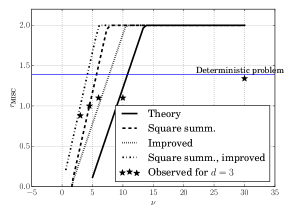
Figure 4: The upper bound of the MISC rate, $r_{\text{MISC}}$, as predicted in Theorem 10 versus the observed rates when running the example detailed in Section 6. Refer to Section 5 for an explanation of the different curves. Also included are the observed convergence rates for a few values of $\nu$ and the observed convergence rate of MISC with no random variable and constant diffusion coefficient, $a$, as a horizontal line. The latter is referred to as the “deterministic problem” and shows more clearly the effect of the logarithmic factor in the work for $d>1$, as shown in Figure 9 and proved in [23, Theorem 1].

6 Numerical experiments

We now verify the effectiveness of the MISC approximation on some instances of the general elliptic equation (1), as well as the validity of the convergence analysis detailed in the previous sections. In particular, we consider the domain $\mathcal{B}=[0,1]^{d}$ and the family of random diffusion coefficients specified in Example 1. In more detail, we consider a problem with one physical dimension ($d=1$) and another with three dimensions ($d=3$); in both cases, we set $\varsigma({{\bm{x}}})=1$, and model the diffusion coefficient by the expansion (8) with different values of $\nu$. Finally, the quantity of interest is a local average defined as

$$F({{\bm{y}}})=\frac{10}{(\sigma\sqrt{2\pi})^{d}}\int_{\mathscr{B}}u({{\bm{x}}},{{\bm{y}}})\exp\left(-\frac{\|{{\bm{x}}}-{{\bm{x}}}_{0}\|_{2}^{2}}{2\sigma^{2}}\right)d{{\bm{x}}}$$ (45)

with $\sigma=0.2$ and location ${{\bm{x}}}_{0}=0.3$ for $d=1$ and ${{\bm{x}}}_{0}=[0.3,0.2,0.6]$ for $d=3$. The deterministic problems are discretized with a second-order centered finite differences scheme for which we expect to recover the same rate in the numerical experiments that we would obtain with piece-wise multi-linear finite elements on a structured mesh. We choose the mesh-sizes in (17) and $h_{0,i}=1/3$ for all $i=1,\ldots,d$, and the resulting linear system is solved with GMRES with sufficient accuracy. With these values and using the coarsest discretization, $h_{0}=1/3$, in all dimensions, the coefficient of variation of the quantity of interest can be approximated to be between $90\%$ and $110\%$ depending on the number of dimensions, $d$, and the particular value of the parameter, $\nu$, that we consider below. Finally, the quadrature points on the stochastic domain are the already-mentioned Clenshaw-Curtis points (see eq. (19) and (20)).

In the plots below, the computational work is compared in terms of the total number of degrees of freedom to avoid discrepancies in running time due to implementation details, i.e., using (27) and Assumption A3. Moreover, we set $\gamma=1$ in (30), which is motivated by the fact that, for the tolerances we are interested in, we estimate that the cost of solving a linear system with GMRES is linear with respect to the number of degrees of freedom.

In order to evaluate the MISC estimator, we need to build the index set (29). To do that, we must be able to evaluate two quantities for every ${{{\bm{\alpha}}}}$ and ${{{\bm{\beta}}}}$: the work contribution, $\Delta W_{{{{\bm{\alpha}}}},{{{\bm{\beta}}}}}$, and the error contribution, $\Delta E_{{{{\bm{\alpha}}}},{{{\bm{\beta}}}}}$. Evaluating the work contribution is straightforward thanks to Assumption A3 and using $\gamma=1$. On the other hand, evaluating the error contribution is more involved. We look at two options:

“brute-force” evaluation.

We compute ${{\bm{\Delta}}}[F_{{{{\bm{\alpha}}}},{{{\bm{\beta}}}}}]$ for all $({{{\bm{\alpha}}}},{{{\bm{\beta}}}})$ within some “universe” index set and set $\Delta E_{{{{\bm{\alpha}}}},{{{\bm{\beta}}}}}=\left|{{\bm{\Delta}}}[F_{{{{\bm{\alpha}}}},{{{\bm{\beta}}}}}]\right|$. Notice that this method is not practical since the cost of constructing the set, $\mathcal{I}$, would far dominate the cost of the MISC estimator. However, within some “universe” index set, this method would produce the best possible convergence and serve as a benchmark for other MISC sets within that universe.

“a-priori” evaluation.

We use Lemma 8 to bound $\Delta E_{{{{\bm{\alpha}}}},{{{\bm{\beta}}}}}$. Using these bounds instead of exact values produces quasi-optimal index sets (cf. [3, 34] ). This method in turn requires the estimation of the parameters $r_{\text{FEM}},\left\{g_{s,j}\right\}_{j\geq 1}$ for all $s=0,\ldots,s_{\max}$. Since we use a second-order centered finite differences scheme and consider the convergence of a quantity of interest, we expect $r_{\text{FEM}}=2\min\left(1,\frac{\nu}{d}\right)$ as motivated by the “improved” analysis in the previous section and considering the summability properties of $\left\{A_{{{\bm{k}}}}^{2}\|D^{{{\bm{s}}}}\Upsilon_{{{\bm{k}}},{{\bm{\ell}}}}\|_{L^{\infty}(\mathscr{B})}^{2}\right\}$. This can also be validated numerically in the usual way by fixing all random variables to their expected value and checking the decay of $\Delta E_{{{{\bm{\alpha}}}},{{\bm{1}}}}$ with respect to ${{{\bm{\alpha}}}}$.

On the other hand, estimating $\left\{g_{s,j}\right\}_{j\geq 1}$ for $s=0,\ldots,s_{\max}$ is more difficult since, in principle, we do not know a priori, for a given ${{{\bm{\alpha}}}}$ and ${{{\bm{\beta}}}}$, which value of $s\in\{0,1,\ldots,s_{\max}\}$ yields the smallest estimate of $\Delta E_{{{{\bm{\alpha}}}},{{{\bm{\beta}}}}}$. Instead, we use a “simplified” model that was used in [23]:

$$\Delta E_{{{{\bm{\alpha}}}},{{{\bm{\beta}}}}}\leq Ce^{-\sum_{j\geq 1}m(\beta_{j}-1)\tilde{g}_{j}}2^{-|{{{\bm{\alpha}}}}|r_{\mathrm{FEM}}},$$ (46)

where $\tilde{g}_{j}$ is some unknown function of $g_{s,j}$ for all $s=0,1,\ldots,s_{\max}$. $\tilde{g}_{j}$ can be estimated given $r_{\text{FEM}}$ and a set of evaluations of $\left|{{\bm{\Delta}}}[F_{{{{\bm{\alpha}}}},{{{\bm{\beta}}}}}]\right|$ for some $({{{\bm{\alpha}}}},{{{\bm{\beta}}}})\in\mathcal{I}^{*}$ by solving a least-squares problem to fit the linear model

$$\sum_{j\geq 1}\tilde{g}_{j}m(\beta_{j}-1)=-\log\left(\left|{{\bm{\Delta}}}[F_{{{{\bm{\alpha}}}},{{{\bm{\beta}}}}}]\right|\right)-|{{{\bm{\alpha}}}}|r_{\text{FEM}},\qquad\text{for all }({{{\bm{\alpha}}}},{{{\bm{\beta}}}})\in\mathcal{I}^{*}.$$

For our example, these rates are plotted in Figures 5(a) and 7(a) for $d=1$ and $d=3$, respectively. In our current implementation, the construction of the optimal MISC set, $\mathcal{I}$, is separate from the set $\mathcal{I}^{*}$. However, it is possible in principle to construct an algorithm in which the optimal MISC set, $\mathcal{I}$, is constructed iteratively by alternating between estimating rates given a set of indices and evaluating the MISC estimator.

Note that, in the current work, there are certain operations whose costs we do not track or compare. The first operation is the estimation of the stochastic rates, $\left\{\tilde{g}_{j}\right\}_{j\geq 1}$. The second operation is the construction of the optimal set given estimates of error and work contribution. We believe that the cost of these two operations can be reduced by using the previously mentioned iterative algorithm. The cost of these operations is thus dominated by the cost of evaluating the MISC estimator. The third operation is the assembly of the stiffness matrix, especially since it scales linearly with the number of random variables. While the cost of this operation is relevant to our discussion, it is usually dominated by the cost of the linear solver, at least for fine-enough discretizations.

Finally, we also compare MISC to the Multi-index Monte Carlo (MIMC) method as detailed in [24], for which ${\mathcal{O}\left(W_{\max}^{-0.5}\right)}$ convergence can be proved for Example 1 with $\gamma=1,d\leq 3$ and sufficiently large $\nu$ (see Appendix A). Moreover, when computing errors, we use the result obtained using a well-resolved MISC solution as a reference value.

Figures 5(b–d) and Figures 7(b–d) compare some computed values of $\left|{{\bm{\Delta}}}[F_{{{{\bm{\alpha}}}},{{{\bm{\beta}}}}}]\right|$ versus the model (46) using the estimated rates $r_{\text{FEM}}=2\min\left(1,\frac{\nu}{d}\right)$ and $\left\{\tilde{g}_{j}\right\}_{j\geq 1}$. These plots show that the model (46) is a good fit for the case $d=1,\nu=2.5$ and $d=3,\nu=4.5$. Moreover, similar plots were produced for other values of $d$ and $\nu$ that are not reported here but also show good fit. Figures 6 and 8 show

• the maximum space discretization level, $\max_{({{{\bm{\alpha}}}},{{{\bm{\beta}}}})\in\mathcal{I}}\max({{{\bm{\alpha}}}})$,

• the maximum quadrature level, $\max_{({{{\bm{\alpha}}}},{{{\bm{\beta}}}})\in\mathcal{I}}\max({{{\bm{\beta}}}})$,

• the index of the last activated random variable, $\max_{({{{\bm{\alpha}}}},{{{\bm{\beta}}}})\in\mathcal{I}}\max_{\beta_{j}>1}j$,

• and the maximum number of jointly activated variables, $\max_{({{{\bm{\alpha}}}},{{{\bm{\beta}}}})\in\mathcal{I}}|{{{\bm{\beta}}}}-{{\bm{1}}}|_{0}$.

These values convey the size of the used index set, $\mathcal{I}$, for different values of $W_{\max}$.

Figure 4 shows the observed convergence rates of MISC vs MIMC for the cases $d=1$ and $d=3$ and different values of $\nu$. This figure shows that the observed rates are better than those predicted by the theory developed in this work, which suggests that further improvement in the theory is possible (see Remark 4). Figures 9 and 10 show in greater details the observed convergence curves for $d=1,\nu=2.5$ and $d=3,\nu=4.5$ and their respective linear fit in log-log scale.

We recall that, as shown in [23, Theorem 1], the convergence rate of MISC with a finite number of random variables is ${\mathcal{O}\left(W_{\max}^{-2}\log(W_{\max})^{d-1}\right)}$. Compare this to the theory presented here that predicts, as $\nu\to\infty$, a convergence of ${\mathcal{O}\left(W_{\max}^{-2+\epsilon}\right)}$ for any $\epsilon>0$. However, Figure 9 shows that even for a problem with $d=3$ and no random variables, MISC (which, in this case, becomes equivalent to a deterministic combination technique [7]) has an observed convergence rate that is closer to $-1.38$. This is due to the effect of the logarithmic term that is nonzero for $d>1$. Based on this, we should not expect a better convergence rate for $d=3$ and any finite $\nu>0$. This is also numerically validated in Figure 10, which shows the full convergence curves for $d=1,\nu=2.5$ and $d=3,\nu=4.5$.

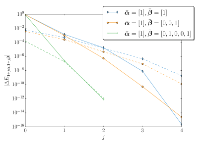
Figure 5: Example 1, $d=1$ and $\nu=2.5$. (a) A plot of the estimated stochastic rates, $\tilde{g}_{j}$, that are used in (46). Different markers correspond to different modes multiplying the same value of $A_{{{\bm{k}}}}$. (b–d) solid lines show the computed approximations of $\Delta E_{{{\bm{1}}},{{\bm{1}}}+j\tilde{{{\bm{\beta}}}}},\Delta E_{{{\bm{1}}}+j\tilde{{{\bm{\alpha}}}},{{\bm{1}}}}$ and $\Delta E_{{{\bm{1}}}+j\tilde{{{\bm{\alpha}}}},{{\bm{1}}}+j\tilde{{{\bm{\beta}}}}}$, respectively versus the model in (46) represented with dashed lines.

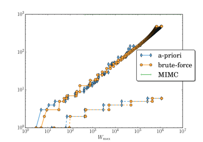
Figure 6: Example 1, $d=1$ and $\nu=2.5$. This figure shows extreme values of ${{{\bm{\alpha}}}}$ and ${{{\bm{\beta}}}}$ included in the MISC set, $\mathcal{I}$. Specifically, the left-solid lines is the maximum space discretization level, $\max_{({{{\bm{\alpha}}}},{{{\bm{\beta}}}})\in\mathcal{I}}\left(\max\left({{{\bm{\alpha}}}}\right)\right)$, the left-dashed lines are the maximum quadrature level, $\max_{({{{\bm{\alpha}}}},{{{\bm{\beta}}}})\in\mathcal{I}}\left(\max\left({{{\bm{\beta}}}}\right)\right)$, the right-solid lines are the index of the last activated random variable, $\max_{({{{\bm{\alpha}}}},{{{\bm{\beta}}}})\in\mathcal{I}}\left(\max_{\beta_{j}>1}j\right)$, and the right-dashed lines are the maximum number of jointly activated variables, $\max_{({{{\bm{\alpha}}}},{{{\bm{\beta}}}})\in\mathcal{I}}\left(|{{{\bm{\beta}}}}-{{\bm{1}}}|_{0}\right)$.

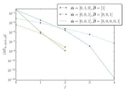
Figure 7: Example 1, $d=3$ and $\nu=4.5$. (a) A plot of the estimated stochastic rates, $\tilde{g}_{j}$, that are used in (46). Here different markers correspond to different modes multiplying the same value of $A_{{{\bm{k}}}}$. (b–d) solid lines show the computed approximations of $\Delta E_{{{\bm{1}}},{{\bm{1}}}+j\tilde{{{\bm{\beta}}}}},\Delta E_{{{\bm{1}}}+j\tilde{{{\bm{\alpha}}}},{{\bm{1}}}}$ and $\Delta E_{{{\bm{1}}}+j\tilde{{{\bm{\alpha}}}},{{\bm{1}}}+j\tilde{{{\bm{\beta}}}}}$, respectively versus the model in (46) represented with dashed lines.

Figure 8: Example 1, $d=3$ and $\nu=4.5$. This figure shows extreme values of ${{{\bm{\alpha}}}}$ and ${{{\bm{\beta}}}}$ included in the MISC set $\mathcal{I}$. Specifically, the left-solid lines are the maximum space discretization level, $\max_{({{{\bm{\alpha}}}},{{{\bm{\beta}}}})\in\mathcal{I}}\left(\max\left({{{\bm{\alpha}}}}\right)\right)$, the left-dashed are the maximum quadrature level, $\max_{({{{\bm{\alpha}}}},{{{\bm{\beta}}}})\in\mathcal{I}}\left(\max\left({{{\bm{\beta}}}}\right)\right)$, the right-solid are the index of the last activated random variable, $\max_{({{{\bm{\alpha}}}},{{{\bm{\beta}}}})\in\mathcal{I}}\left(\max_{\beta_{j}>1}j\right)$, and the right-dashed are the maximum number of jointly activated variables, $\max_{({{{\bm{\alpha}}}},{{{\bm{\beta}}}})\in\mathcal{I}}\left(|{{{\bm{\beta}}}}-{{\bm{1}}}|_{0}\right)$.

(a) $d=1$

(b) $d=3$

Figure 9: Convergence results of MISC Example 1 with a constant diffusion coefficient, $a$. In this case, MISC is equivalent to a deterministic combination technique [7]. These plots shows the non-asymptotic effect of the logarithmic factor for $d>1$ (as discussed in [23, Theorem 1]) on the linear convergence fit in log-log scale.

(a) $d=1,\nu=2.5$

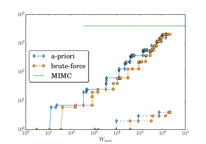
(b) $d=3,\nu=4.5$

Figure 10: Convergence results of MISC vs MIMC when applied to Example 1.

7 Conclusions

In this work, we analyzed the performance of the MISC method when applied to linear elliptic PDEs depending on a countable sequence of random variables. For ease of presentation, we worked on tensor product domains, but the results can be extended to more general domains and non-uniform meshes, as briefly mentioned Section 3. We proved a convergence result using a summability argument that shows that, in certain cases, the convergence of the method is essentially dictated by the convergence properties of the deterministic solver. We then applied the convergence theorem to derive convergence rates for the approximation of the expected value of a functional of the solution of an elliptic PDE with diffusion coefficient described by a random field, tracking the dependence of the convergence rate on the spatial regularity of the realizations of the random field. The theoretical findings are backed up by numerical experiments that show the dependence of the convergence rate on the regularity parameter. Future works includes extending the convergence analysis to higher-order finite element solvers and improving the estimates of the error contribution of each difference operator by taking into account the factorial terms appearing in the estimates for the size of the Chebyshev coefficients, cf. [3, 11]. Moreover, the ideas in [12] can be extended to design an algorithm that iteratively estimates the optimal MISC set by alternating between optimizing the set and evaluating the estimator to ensure that the work to optimize the set is dominated by the work to evaluate the MISC estimator.

Acknowledgement

F. Nobile and L. Tamellini received support from the Center for ADvanced MOdeling Science (CADMOS) and partial support by the Swiss National Science Foundation under the Project No. 140574 “Efficient numerical methods for flow and transport phenomena in heterogeneous random porous media”. L. Tamellini also received support from the Gruppo Nazionale Calcolo Scientifico - Istituto Nazionale di Alta Matematica “Francesco Severi” (GNCS-INDAM). R. Tempone is a member of the KAUST Strategic Research Initiative, Center for Uncertainty Quantification in Computational Sciences and Engineering. R. Tempone received support from the KAUST CRG3 Award Ref: 2281.

Appendix A Summability of series expansion

We start by recalling a useful multivariate Faà di Bruno formula taken from [13, Theorem 2.1].

Lemma 11.

Let $\mathscr{B}\subset\mathbb{R}^{d}$ be an open domain, $g:\mathscr{B}\rightarrow\mathbb{R}$ and $f:\mathbb{R}\rightarrow\mathbb{R}$ be functions of class $C^{s}$ and denote $h=f\circ g:\mathscr{B}\rightarrow\mathbb{R}$. For any multi-index ${{\bm{i}}}\in\mathbb{N}^{d}$, $|{{\bm{i}}}|\leq s$, and any ${{\bm{x}}}\in\mathscr{B}$,

$$D^{{\bm{i}}}h({{\bm{x}}})={{\bm{i}}}!\sum_{\lambda=1}^{|{{\bm{i}}}|}f^{(\lambda)}(g({{\bm{x}}}))\sum_{r=1}^{\lambda}\sum_{p_{r}({{\bm{i}}},\lambda)}\prod_{j=1}^{r}\frac{(D^{\bm{\ell}_{j}}g({{\bm{x}}}))^{k_{j}}}{k_{j}!(\bm{\ell}_{j}!)^{k_{j}}},$$ (47)

holds, where

$$p_{r}({{\bm{i}}},\lambda)=\{(k_{j},\bm{\ell}_{j})\in\mathbb{N}\times\mathbb{N}^{d}_{0},\;j=1,\ldots,r:\;\;\bm{0}\prec\bm{\ell}_{1}\prec\bm{\ell}_{2}\prec\cdots\prec\bm{\ell}_{r},\;\sum_{j=1}^{r}k_{j}=\lambda,\;\;\sum_{j=1}^{r}k_{j}\bm{\ell}_{j}={{\bm{i}}}\}$$

and $\prec$ denotes the lexicographic ordering of multi-indices. The set $p_{r}({{\bm{i}}},\lambda)$ denotes the set of possible decompositions of ${{\bm{i}}}$ as a sum of $\lambda$ multi-indices with $r\leq\lambda$ distinct multi-indices, $\bm{\ell}_{j}$, taken with multiplicity $k_{j}$ such that $\sum_{j=1}^{r}k_{j}=\lambda$.

Also from [13, Corollary 2.9], we have that, for any ${{\bm{i}}}\in\mathbb{N}^{d}$,

$${{\bm{i}}}!\sum_{r=1}^{\lambda}\sum_{p_{r}({{\bm{i}}},\lambda)}\prod_{j=1}^{r}\frac{1}{k_{j}!(\bm{\ell}_{j}!)^{k_{j}}}=S_{|{{\bm{i}}}|,\lambda},$$

where $S_{n,k}$ is the Stirling number of the second kind, which counts the number of ways to partition a set of $n$ objects into $k$ non-empty subsets. Similarly, the Bell number, $B_{n}=\sum_{k=0}^{n}S_{n,k}$, counts the number of partitions of a set of $n$ objects, whereas the ordered Bell numbers are defined by $\tilde{B}_{n}=\sum_{k=0}^{n}k!S_{n,k}$ and satisfy the recursive relation $\tilde{B}_{n}=\sum_{k=0}^{n-1}\binom{n}{k}\tilde{B}_{k}$. Clearly, $B_{n}\leq\tilde{B}_{n}$. Moreover, the bound

$$B_{n}\leq\tilde{B}_{n}\leq n!/(\log 2)^{n}$$ (48)

was given in [3, Lemma A.3]. We now use these results to show the following result

Lemma 12.

Let $\mathscr{B}\subset\mathbb{R}^{d}$ be an open-bounded domain and $\kappa\in C^{s}(\overline{\mathscr{B}})$ (real or complex valued) for $s\geq 0$. Then, $a=e^{\kappa}\in C^{s}(\overline{\mathscr{B}})$ and we have the estimate

$$\|a\|_{C^{s}(\overline{\mathscr{B}})}\leq\frac{s!}{(\log 2)^{s}}\|a\|_{C^{0}(\overline{\mathscr{B}})}(1+\|\kappa\|_{C^{s}(\overline{\mathscr{B}})})^{s}.$$

Proof.

Using formula (47) we have for any ${{\bm{i}}}\in\mathbb{N}^{d}$, $|{{\bm{i}}}|\leq s$ and any ${{\bm{x}}}\in\mathscr{B}$

$$|D^{{\bm{i}}}e^{\kappa({{\bm{x}}})}| ={{\bm{i}}}!\sum_{\lambda=1}^{|{{\bm{i}}}|}e^{\kappa({{\bm{x}}})}\sum_{r=1}^{\lambda}\sum_{p_{r}({{\bm{i}}},\lambda)}\prod_{j=1}^{r}\frac{|D^{\bm{\ell}_{j}}\kappa({{\bm{x}}})|^{k_{j}}}{k_{j}!(\bm{\ell}_{j}!)^{k_{j}}}\leq\|a\|_{C^{0}(\overline{\mathscr{B}})}\sum_{\lambda=1}^{|{{\bm{i}}}|}\|\kappa\|_{C^{s}(\overline{\mathscr{B}})}^{\lambda}S_{|{{\bm{i}}}|,\lambda}$$

$$\leq\|a\|_{C^{0}(\overline{\mathscr{B}})}(1+\|\kappa\|_{C^{s}(\overline{\mathscr{B}})})^{|{{\bm{i}}}|}B_{n}.$$

The result then follows from the bound on the Bell numbers in (48). ∎

A.1 $L^{p}(\Gamma)$ summability, pointwise in space

We now consider a diffusion coefficient as in Assumption A2:

$$a({{\bm{x}}},{{\bm{y}}})=\exp\left\{\sum_{j\geq 1}\psi_{j}({{\bm{x}}})y_{j}\right\}=\prod_{j=1}^{\infty}e^{y_{j}\psi_{j}({{\bm{x}}})},\qquad{{\bm{x}}}\in\mathscr{B},$$

with $y_{j}$, $j\geq 1$, independent random variables, all uniformly distributed in $[-1,1]$ and recall the definition of the sequence ${{\bm{b}}}_{s}=\{b_{s,j}\}_{j\geq 1}$, for all $s\in\mathbb{N}$ in (6).

Lemma 13.

If ${{\bm{b}}}_{0}\in\ell^{2}$ then ${\mathbb{E}\mspace{-2.0mu}\left[a({{\bm{x}}})^{p}\right]}<\infty$ for all $0<p<\infty$ and $\forall{{\bm{x}}}\in\mathscr{B}$.

Proof.

For any ${{\bm{x}}}\in\mathscr{B}$, we estimate the $p$-th moment of $a({{\bm{x}}},{{\bm{y}}})$, exploiting independence of the random variables, $y_{j}$:

$${\mathbb{E}\mspace{-2.0mu}\left[a({{\bm{x}}})^{p}\right]}={\mathbb{E}\mspace{-2.0mu}\left[\prod_{j=1}^{\infty}e^{py_{j}\psi_{j}({{\bm{x}}})}\right]}=\prod_{j=1}^{\infty}{\mathbb{E}\mspace{-2.0mu}\left[e^{py_{j}\psi_{j}({{\bm{x}}})}\right]}=\prod_{j=1}^{\infty}\frac{\sinh(p\psi_{j}({{\bm{x}}}))}{p\psi_{j}({{\bm{x}}})}=\exp\left\{\sum_{j=1}^{\infty}\log\left(\frac{\sinh(p\psi_{j}({{\bm{x}}}))}{p\psi_{j}({{\bm{x}}})}\right)\right\}$$

where in the last two equalities we have implicitly assumed that $\sinh(z)/z=1$ for $z=0$. Setting $\theta_{0}(p;{{\bm{x}}})=\prod_{j=1}^{\infty}\frac{\sinh(p\psi_{j}({{\bm{x}}}))}{p\psi_{j}({{\bm{x}}})}$ and observing that $\log(\sinh(z)/z)\sim z^{2}/6$, we have

$${\mathbb{E}\mspace{-2.0mu}\left[a({{\bm{x}}})^{p}\right]}=\theta_{0}(p;{{\bm{x}}})<\infty\quad\forall{{\bm{x}}}\in\mathscr{B},\;\;0<p<\infty\qquad\Longleftrightarrow\qquad\sum_{j=1}^{\infty}\psi_{j}({{\bm{x}}})^{2}<\infty.$$

Since $\sum_{j=1}^{\infty}b_{0,j}^{2}<\infty$ implies $\sum_{j=1}^{\infty}\psi_{j}({{\bm{x}}})^{2}<\infty$ for any ${{\bm{x}}}\in\mathscr{B}$, this concludes the proof. ∎

A similar result holds for higher-order derivatives of $a$.

Lemma 14.

Let $s\in\mathbb{N}_{+}$. If ${{\bm{b}}}_{s}\in\ell^{2}$, then for any ${{\bm{i}}}\in\mathbb{N}^{d}$, $|{{\bm{i}}}|=s$, ${\mathbb{E}\mspace{-2.0mu}\left[(D^{{\bm{i}}}a({{\bm{x}}}))^{2p}\right]}<\infty$ for all $0<p<\infty$ and $\forall{{\bm{x}}}\in\mathscr{B}$.

Proof.

Since the calculations are tedious, we prove the result here for $s=1$ only. Using the chain rule, we have

$$(\partial_{x_{i}}a({{\bm{x}}},{{\bm{y}}}))^{2p} =\left(\sum_{j\geq 1}a({{\bm{x}}},{{\bm{y}}})\partial_{x_{i}}\psi_{j}({{\bm{x}}})y_{j}\right)^{2p}=a({{\bm{x}}},{{\bm{y}}})^{2p}\sum_{{{\bm{q}}}\in\mathbb{N}^{\mathbb{N}}\atop|{{\bm{q}}}|=2p}(2p)!\prod_{j=1}^{\infty}\frac{1}{q_{j}!}(\partial_{x_{i}}\psi_{j}({{\bm{x}}})y_{j})^{q_{j}}$$

$$=\sum_{{{\bm{q}}}\in\mathbb{N}^{\mathbb{N}}\atop|{{\bm{q}}}|=2p}(2p)!\prod_{j=1}^{\infty}\frac{1}{q_{j}!}(\partial_{x_{i}}\psi_{j}({{\bm{x}}})y_{j})^{q_{j}}e^{2py_{j}\psi_{j}({{\bm{x}}})}.$$

Hence,

$${\mathbb{E}\mspace{-2.0mu}\left[(\partial_{x_{i}}a({{\bm{x}}},{{\bm{y}}}))^{2p}\right]}=\sum_{{{\bm{q}}}\in\mathbb{N}^{\mathbb{N}}\atop|{{\bm{q}}}|=2p}(2p)!\prod_{j=1}^{\infty}(\partial_{x_{i}}\psi_{j}({{\bm{x}}}))^{q_{j}}{\mathbb{E}\mspace{-2.0mu}\left[\frac{1}{q_{j}!}y_{j}^{q_{j}}e^{2py_{j}\psi_{j}({{\bm{x}}})}\right]}.$$

We now distinguish between even or odd $q_{j}$. For even $q_{j}$, we have

$${\mathbb{E}\mspace{-2.0mu}\left[\frac{1}{q_{j}!}y_{j}^{q_{j}}e^{2py_{j}\psi_{j}({{\bm{x}}})}\right]}\leq{\mathbb{E}\mspace{-2.0mu}\left[\frac{1}{q_{j}!}e^{2py_{j}\psi_{j}({{\bm{x}}})}\right]}=\frac{1}{q_{j}!}\frac{\sinh(2p\psi_{j}({{\bm{x}}}))}{2p\psi_{j}({{\bm{x}}})}$$

while for $q_{j}$ odd we have

$${\mathbb{E}\mspace{-2.0mu}\left[\frac{1}{q_{j}!}y_{j}^{q_{j}}e^{2py_{j}\psi_{j}({{\bm{x}}})}\right]} =\frac{1}{q_{j}!}\int_{-1}^{1}\frac{1}{2}y^{q_{j}}e^{2py\psi_{j}({{\bm{x}}})}dy=\frac{1}{q_{j}!}\int_{0}^{1}y^{q_{j}}\sinh(2py\psi_{j}({{\bm{x}}}))dy$$

$$=\frac{1}{q_{j}!}\sum_{n=0}^{\infty}\frac{(2p\psi_{j}({{\bm{x}}}))^{2n+1}}{(2n+1)!}\int_{0}^{1}y^{2n+1+q_{j}}dy=\frac{1}{q_{j}!}\sum_{n=0}^{\infty}\frac{(2p\psi_{j}({{\bm{x}}}))^{2n+1}}{(2n+1)!(2n+2+q_{j})}$$

$$\leq\frac{1}{(q_{j}+1)!}\sinh(2p|\psi_{j}({{\bm{x}}})|)\leq\frac{2pb_{1,j}}{(q_{j}+1)!}\frac{\sinh(2p\psi_{j}({{\bm{x}}}))}{2p\psi_{j}({{\bm{x}}})}.$$

Hence, defining the function

$$f(q_{j})=\begin{cases}\frac{1}{q_{j}!}&\text{for $q_{j}$ even},\\[2.84526pt] \frac{2pb_{1,j}}{(q_{j}+1)!}&\text{for $q_{j}$ odd},\end{cases}$$

we have

$${\mathbb{E}\mspace{-2.0mu}\left[(\partial_{x_{i}}a({{\bm{x}}},{{\bm{y}}}))^{2p}\right]} \leq\sum_{{{\bm{q}}}\in\mathbb{N}^{\mathbb{N}}\atop|{{\bm{q}}}|=2p}(2p)!\prod_{j=1}^{\infty}b_{1,j}^{q_{j}}f(q_{j})\frac{\sinh(2p\psi_{j}({{\bm{x}}}))}{2p\psi_{j}({{\bm{x}}})}=\theta_{0}(2p;{{\bm{x}}})\sum_{{{\bm{q}}}\in\mathbb{N}^{\mathbb{N}}\atop|{{\bm{q}}}|=2p}(2p)!\prod_{j=1}^{\infty}b_{1,j}^{q_{j}}f(q_{j})$$

$$\leq\theta_{0}(2p;{{\bm{x}}})\sum_{{{\bm{q}}}\in\mathbb{N}^{\mathbb{N}}\atop|{{\bm{q}}}|=2p,\text{${{\bm{q}}}$ even}}(2p)!(1+2p)^{|{{\bm{q}}}|_{0}}\prod_{j=1}^{\infty}\frac{b_{1,j}^{q_{j}}}{q_{j}!}$$

$$\leq(1+2p)^{p}\theta_{0}(2p;{{\bm{x}}})\sum_{{{\bm{q}}}\in\mathbb{N}^{\mathbb{N}}\atop|{{\bm{q}}}|=p}(2p)!\prod_{j=1}^{\infty}\frac{b_{1,j}^{2q_{j}}}{(2q_{j})!}$$

$$\leq(1+2p)^{p}(2p)^{p}\theta_{0}(2p;{{\bm{x}}})\sum_{{{\bm{q}}}\in\mathbb{N}^{\mathbb{N}}\atop|{{\bm{q}}}|=p}p!\prod_{j=1}^{\infty}\frac{(b_{1,j}^{2})^{q_{j}}}{q_{j}!}=(1+2p)^{p}(2p)^{p}\theta_{0}(2p;{{\bm{x}}})\left(\sum_{j\geq 1}b_{1,j}^{2}\right)$$

from which we see that ${\mathbb{E}\mspace{-2.0mu}\left[(\partial_{x_{i}}a({{\bm{x}}},{{\bm{y}}}))^{2p}\right]}$ is bounded for any $0\leq p<\infty$ and any ${{\bm{x}}}\in\mathscr{B}$ if ${{\bm{b}}}_{1}\in\ell^{2}$. ∎

A.2 $L^{p}(\Gamma)$ summability, uniform in space

Assuming now that ${{\bm{b}}}_{s}\in\ell^{2}$ so that the random field, $a$, is $s$-times differentiable in an $L^{p}(\Gamma)$ sense according to Lemma 14, we show that this implies some uniform $L^{p}(\Gamma)$ summability as detailed in the next lemma.

Lemma 15.

Let $s\in\mathbb{N}_{+}$. If ${{\bm{b}}}_{s}\in\ell^{2}$ then ${\mathbb{E}\mspace{-2.0mu}\left[\|a\|^{p}_{W^{\upsilon,\infty}(\mathscr{B})}\right]}<\infty$ for all $1\leq p<\infty$ and $\upsilon<s$.

Proof.

We exploit the Sobolev embedding, $W^{\upsilon+\frac{d}{2q},2q}(\mathscr{B})\subseteq W^{\upsilon,\infty}(\mathscr{B})$, for all $\upsilon\geq 0$ and $q\geq 1$. For $q\geq\max\{d/2(s-\upsilon),p/2\}$, we have

$${\mathbb{E}\mspace{-2.0mu}\left[\|a\|^{p}_{W^{\upsilon,\infty}(\mathscr{B})}\right]} \leq{\mathbb{E}\mspace{-2.0mu}\left[\|a\|^{2q}_{W^{s-\frac{d}{2q},\infty}(\mathscr{B})}\right]}\lesssim{\mathbb{E}\mspace{-2.0mu}\left[\|a\|^{2q}_{W^{s,2q}(\mathscr{B})}\right]}={\mathbb{E}\mspace{-2.0mu}\left[\sum_{|{{\bm{i}}}|\leq s}\int_{\mathscr{B}}(D^{{\bm{i}}}a({{\bm{x}}}))^{2q}d{{\bm{x}}}\right]}$$

$$=\sum_{|{{\bm{i}}}|\leq s}\int_{\mathscr{B}}{\mathbb{E}\mspace{-2.0mu}\left[(D^{{\bm{i}}}a({{\bm{x}}}))^{2q}\right]}d{{\bm{x}}}<\infty,$$

where the last term is bounded from Lemma 14. ∎

Now, we directly observe by taking $\upsilon=0$ in the previous result that $a_{\max}=\|a\|_{L^{\infty}(\mathscr{B})}$ has bounded moments,

$${\mathbb{E}\mspace{-2.0mu}\left[a_{\max}^{p}\right]}<\infty,$$

for all $1\leq p<\infty$ and $0<s$. Finally, by observing that, due to the construction (2) in Assumption A2, we have that $a_{\min}=\frac{1}{\|a^{-1}\|_{L^{\infty}(\mathscr{B})}}$ has the same distribution as $a_{\max}$. As a consequence, $a_{\min}$ has bounded moments as well. This implies in turn that (3) holds and thus problem (1) is well posed in the Bochner space, $L^{p}\left(\Gamma;H^{1}_{0}(\mathscr{B})\right)$. That is,

Corollary 16 (Well posedness with log uniform coefficient).

We have for $0<\nu$ that the problem in Example 1 is well posed in the Bochner space $L^{p}\left(\Gamma;H^{1}_{0}(\mathscr{B})\right)$. The corresponding solution, $u$, satisfies

$$\|u\|_{L^{p}(\Gamma;H^{1}_{0}(\mathscr{B}))}\leq C{\mathbb{E}\mspace{-2.0mu}\left[\frac{1}{a_{\min}^{p}}\right]}^{1/p}\|f\|_{H^{-1}(\mathscr{B})}.$$

We observe that higher regularity of the solution, $u$, can be obtained by using larger values of $s$ in Lemma 15. This in turn yields control on moments of $W^{\upsilon,\infty}(\mathscr{B})$ norms of the coefficient, $a$, and following, for instance, estimates similar to (2.10) in [18, Theorem 2.4], we can estimate moments of the $H^{1+s}(\mathscr{B})$ norm of the solution, $u$. These regularity estimates, once combined with pathwise error estimates for the combination technique, can be further used to show the corresponding $\nu$-dependent convergence rates of MIMC [24] for Example 1, similar to what was presented in Section 5 for MISC in the current work.

Appendix B Shift theorem for problem (1)

Here, we seek to establish a shift theorem for the problem

$$\begin{cases}-\textnormal{div}(a({{\bm{x}}})\,\nabla u({{\bm{x}}}))=\varsigma({{\bm{x}}})&\mbox{in}\quad\mathscr{B}=[0,1]^{D}\\ u({{\bm{x}}})\,=\,0&\mbox{on}\quad\partial\mathscr{B},\end{cases}$$ (49)

under suitable assumptions on $a$ and $\varsigma$.

With respect to problem (1), for convenience, we drop the dependence on the parameter vector, ${{\bm{y}}}$. We consider an odd periodic extension of $\varsigma$, on $[-1,1]^{D}$, and an even periodic extension of the coefficient $a$ on $[-1,1]^{D}$, named, respectively, $\tilde{\varsigma}$ and $\tilde{a}$. More precisely, for ${{\bm{j}}}=\{0,1\}^{D}$, we denote by ${{\bm{x}}}_{{\bm{j}}}=((-1)^{j_{1}}x_{1},\ldots,(-1)^{j_{D}}x_{D})$ and

$$\tilde{\varsigma}({{\bm{x}}}_{{\bm{j}}}+2{{\bm{k}}})=(-1)^{|{{\bm{j}}}|}\varsigma({{\bm{x}}}),\qquad\tilde{a}({{\bm{x}}}_{{\bm{j}}}+2{{\bm{k}}})=a({{\bm{x}}}),\qquad\forall{{\bm{x}}}\in[0,1]^{2},\;\;{{\bm{j}}}\in\{0,1\}^{D},\;\;{{\bm{k}}}\in\mathbb{N}^{D}.$$

The following Shift theorem holds for problem (49).

Lemma 17.

If the coefficient $a$ is such that its periodic extension satisfies $\tilde{a}\in W^{s,\infty}(\mathbb{R}^{D})$, $s\geq 0$ and $\varsigma\in C^{\infty}_{0}(\mathscr{B})$ then $u\in H^{s+1}(\mathscr{B})$.

Proof.

We define the extended problem

$$\begin{cases}-\textnormal{div}(\tilde{a}({{\bm{x}}})\,\nabla\tilde{u}({{\bm{x}}}))=\tilde{\varsigma}({{\bm{x}}})&\mbox{in}\quad\tilde{\mathscr{B}}=[-1,1]^{D}\\ \int_{\tilde{\mathscr{B}}}u({{\bm{x}}})\,=\,0\\ \text{periodic boundary conditions on $\partial\tilde{\mathscr{B}}$}.\end{cases}$$

Since by assumption $\tilde{a}\in L^{\infty}(\mathbb{R}^{D})$ and $\tilde{\varsigma}\in L^{2}(\tilde{\mathscr{B}})$, this problem has a unique solution, $\tilde{u}\in H^{1}_{per}(\tilde{\mathscr{B}})\setminus\mathbb{R}$, where we denote with $H^{s}_{per}(\tilde{\mathscr{B}})$ the space of periodic functions with (periodic) square integrable derivatives up to order $s$. It is easy to check that the solution $\tilde{u}$ is odd, that is $\tilde{u}({{\bm{x}}}_{{\bm{j}}})=(-1)^{{{\bm{j}}}}\tilde{u}({{\bm{x}}})$, $\forall{{\bm{x}}}\in[0,1]^{D}$, hence $\tilde{u}=0$ (in the sense of traces) on $\partial\mathscr{B}$ and it coincides with the (unique) solution of (49) on $\mathscr{B}$. Moreover, standard elliptic regularity argumentsallow us to say that $\tilde{u}\in H^{s}_{per}(\tilde{\mathscr{B}})$, hence $u\in H^{s}(\mathscr{B})$. ∎

References

- [1] I. Babuška, F. Nobile, and R. Tempone, A stochastic collocation method for elliptic partial differential equations with random input data, SIAM Review, 52 (2010), 317–355.
- [2] A. Barth, C. Schwab, and N. Zollinger, Multi-level Monte Carlo finite element method for elliptic PDEs with stochastic coefficients, Numerische Mathematik, 119 (2011), 123–161.
- [3] J. Beck, F. Nobile, L. Tamellini, and R. Tempone, On the optimal polynomial approximation of stochastic PDEs by Galerkin and collocation methods, Mathematical Models and Methods in Applied Sciences, 22 (2012), 1250023.
- [4] M. Bieri, A sparse composite collocation finite element method for elliptic SPDEs., SIAM Journal on Numerical Analysis, 49 (2011), 2277–2301.
- [5] V. I. Bogachev, Measure Theory, Vol. 1, Springer Berlin Heidelberg, 2007.
- [6] H. J. Bungartz and M. Griebel, Sparse grids, Acta Numerica, 13 (2004), 147–269.
- [7] H. J. Bungartz, M. Griebel, D. Röschke, and C. Zenger, Pointwise convergence of the combination technique for the Laplace equation, East-West Journal of Numerical Mathematics, 2 (1994), 21–45.
- [8] J. Charrier, Strong and weak error estimates for elliptic partial differential equations with random coefficients, SIAM Journal on Numerical Analysis, 50 (2012), 216–246.
- [9] J. Charrier, R. Scheichl, and A. Teckentrup, Finite element error analysis of elliptic pdes with random coefficients and its application to multilevel Monte Carlo methods, SIAM Journal on Numerical Analysis, 51 (2013), 322–352.
- [10] A. Chkifa, On the lebesgue constant of leja sequences for the complex unit disk and of their real projection, Journal of Approximation Theory, 166 (2013), 176–200.
- [11] A. Cohen, R. Devore, and C. Schwab, Analytic regularity and polynomial approximation of parametric and stochastic elliptic PDE’S, Analysis and Applications, 9 (2011), 11–47.
- [12] N. Collier, A.-L. Haji-Ali, F. Nobile, E. von Schwerin, and R. Tempone, A continuation multilevel Monte Carlo algorithm, BIT Numerical Mathematics, 55 (2015), 399–432.
- [13] G. M. Constantine and T. H. Savits, A multivariate Faà di Bruno formula with applications, Transactions of the American Mathematical Society, 348 (1996), 503–520.
- [14] D. Dũng and M. Griebel, Hyperbolic cross approximation in infinite dimensions, Journal of Complexity, DOI: 10.1016/j.jco.2015.09.006.
- [15] B. Ganapathysubramanian and N. Zabaras, Sparse grid collocation schemes for stochastic natural convection problems, jcp, 225 (2007), 652–685.
- [16] M. B. Giles, Multilevel Monte Carlo path simulation, Operations Research, 56 (2008), 607–617.
- [17] W. J. Gordon and C. A. Hall, Construction of curvilinear co-ordinate systems and applications to mesh generation, International Journal for Numerical Methods in Engineering, 7 (1973), 461–477.
- [18] I. G. Graham, R. Scheichl, and E. Ullmann, Mixed finite element analysis of lognormal diffusion and multilevel Monte Carlo methods, Stochastic Partial Differential Equations: Analysis and Computations, (2015), 1–35.
- [19] M. Griebel and H. Harbrecht, On the convergence of the combination technique, in Sparse Grids and Applications - Munich 2012, J. Garcke and D. Pflüger, eds., vol. 97 of Lecture Notes in Computational Science and Engineering, Springer International Publishing, 2014, 55–74.
- [20] M. Griebel, H. Harbrecht, and M. Peters, Multilevel quadrature for elliptic parametric partial differential equations on non-nested meshes, arXiv preprint arxiv:1509.09058, 2015.
- [21] M. Griebel and S. Knapek, Optimized general sparse grid approximation spaces for operator equations, Mathematics of Computation, 78 (2009), 2223–2257.
- [22] M. Griebel, M. Schneider, and C. Zenger, A combination technique for the solution of sparse grid problems, in Iterative Methods in Linear Algebra, P. de Groen and R. Beauwens, eds., IMACS, Elsevier, North Holland, 1992, pp. 263–281.
- [23] A.-L. Haji-Ali, F. Nobile, L. Tamellini, and R. Tempone, Multi-index stochastic collocation for random PDEs, Computer Methods in Applied Mechanics and Engineering, DOI: 10.1016/j.cma.2016.03.029.
- [24] A.-L. Haji-Ali, F. Nobile, and R. Tempone, Multi-index Monte Carlo: when sparsity meets sampling, Numerische Mathematik, 132 (2015), 767–806.
- [25] A.-L. Haji-Ali, F. Nobile, E. von Schwerin, and R. Tempone, Optimization of mesh hierarchies in multilevel Monte Carlo samplers, Stochastic Partial Differential Equations: Analysis and Computations, 4 (2015), 76–112.
- [26] H. Harbrecht, M. Peters, and M. Siebenmorgen, On multilevel quadrature for elliptic stochastic partial differential equations, in Sparse Grids and Applications, vol. 88 of Lecture Notes in Computational Science and Engineering, Springer, 2013, 161–179.
- [27] M. Hegland, J. Garcke, and V. Challis, The combination technique and some generalisations, Linear Algebra and its Applications, 420 (2007), 249–275.
- [28] S. Heinrich, Multilevel Monte Carlo methods, in Large-Scale Scientific Computing, vol. 2179 of Lecture Notes in Computer Science, Springer Berlin Heidelberg, 2001, 58–67.
- [29] T. J. R. Hughes, J. A. Cottrell, and Y. Bazilevs, Isogeometric analysis: CAD, finite elements, nurbs, exact geometry and mesh refinement, Computer Methods in Applied Mechanics and Engineering, 194 (2005), 4135–4195.
- [30] F. Y. Kuo, C. Schwab, and I. Sloan, Multi-level Quasi-Monte Carlo Finite Element Methods for a Class of Elliptic PDEs with Random Coefficients, Foundations of Computational Mathematics, 15 (2015), 411–449.
- [31] S. Martello and P. Toth, Knapsack problems: algorithms and computer implementations, Wiley-Interscience series in discrete mathematics and optimization, J. Wiley & Sons, 1990.
- [32] A. Narayan and J. D. Jakeman, Adaptive Leja Sparse Grid Constructions for Stochastic Collocation and High-Dimensional Approximation, SIAM Journal on Scientific Computing, 36 (2014), A2952–A2983.
- [33] F. Nobile, L. Tamellini, and R. Tempone, Comparison of Clenshaw-Curtis and Leja Quasi-Optimal Sparse Grids for the Approximation of Random PDEs, in Spectral and High Order Methods for Partial Differential Equations - ICOSAHOM ’14, R. M. Kirby, M. Berzins, and J. S. Hesthaven, eds., vol. 106 of Lecture Notes in Computational Science and Engineering, Springer International Publishing, 2015, 475–482.
- [34] , Convergence of quasi-optimal sparse-grid approximation of Hilbert-space-valued functions: application to random elliptic PDEs, Numerische Mathematik, DOI: 10.1007/s00211-015-0773-y.
- [35] F. Nobile, R. Tempone, and C. Webster, An anisotropic sparse grid stochastic collocation method for partial differential equations with random input data, SIAM Journal on Numerical Analysis, 46 (2008), 2411–2442.
- [36] , A sparse grid stochastic collocation method for partial differential equations with random input data, SIAM Journal on Numerical Analysis, 46 (2008), 2309–2345.
- [37] C. Schillings and C. Schwab, Sparse, adaptive Smolyak quadratures for Bayesian inverse problems, Inverse Problems, 29 (2013), 065011.
- [38] A. Teckentrup, P. Jantsch, C. G. Webster, and M. Gunzburger, A Multilevel Stochastic Collocation Method for Partial Differential Equations with Random Input Data, SIAM/ASA Journal on Uncertainty Quantification, 3 (2015), 1046–1074.
- [39] H. W. van Wyk, Multilevel sparse grid methods for elliptic partial differential equations with random coefficients, arXiv preprint arXiv:1404.0963, 2014.
- [40] G. W. Wasilkowski and H. Wozniakowski, Explicit cost bounds of algorithms for multivariate tensor product problems, Journal of Complexity, 11 (1995), 1–56.
- [41] D. Xiu and J. Hesthaven, High-order collocation methods for differential equations with random inputs, SIAM Journal on Scientific Computing, 27 (2005), 1118–1139.
- [42] C. Zenger, Sparse grids, in Parallel Algorithms for Partial Differential Equations, W. Hackbusch, ed., vol. 31 of Notes on Numerical Fluid Mechanics, Vieweg, 1991, pp. 241–251.