Learning the Dimensionality of Word Embeddings

Abstract

We describe a method for learning word embeddings with data-dependent dimensionality. Our Stochastic Dimensionality Skip-Gram (SD-SG) and Stochastic Dimensionality Continuous Bag-of-Words (SD-CBOW) are nonparametric analogs of Mikolov et al.’s (2013) well-known ‘word2vec’ models. Vector dimensionality is made dynamic by employing techniques used by Côté & Larochelle (2016) to define an RBM with an infinite number of hidden units. We show qualitatively and quantitatively that the SD-SG and SD-CBOW are competitive with their fixed-dimension counterparts while providing a distribution over embedding dimensionalities, which offers a window into how semantics distribute across dimensions.

1 Introduction

Word Embeddings (WEs) (Bengio et al., 2003; Mnih and Hinton, 2009; Turian et al., 2010; Mikolov et al., 2013) have received wide-spread attention for their ability to capture surprisingly detailed semantic information without supervision. However, despite their success, WEs still have deficiencies. One flaw is that the embedding dimensionality must be set by the user and thus requires some form of cross-validation be performed. Yet, this issue is not just one of implementation. Words naturally vary in their semantic complexity, and since vector dimensionality is standardized across the vocabulary, it is difficult to allocate an appropriate number of parameters to each word. For instance, the meaning of the word race varies with context (ex: competition vs anthropological classification), but the meaning of regatta is rather specific and invariant. It seems unlikely that race and regatta’s representations could contain the same number of parameters without one overfitting or underfitting.

To better capture the semantic variability of words, we propose a novel extension to the popular Skip-Gram and Continuous Bag-of-Words models (Mikolov et al., 2013) that allows vectors to have stochastic, data-dependent dimensionality. By employing the same mathematical tools that allow the definition of an Infinite Restricted Boltzmann Machine (Côté and Larochelle, 2016), we define two log-bilinear energy-based models named Stochastic Dimensionality Skip-Gram (SD-SG) and Stochastic Dimensionality Continuous Bag-of-Words (SD-CBOW) after their fixed dimensional counterparts. During training, SD-SG and SD-CBOW allow word representations to grow naturally based on how well they can predict their context. This behavior, among other things, enables the vectors of specific words to use few dimensions (since their context is reliably predictable) and the vectors of vague or polysemous words to elongate to capture as wide a semantic range as needed. As far as we are aware, this is the first word embedding method that allows vector dimensionality to be learned and to vary across words.

2 Fixed Dimension Word Embeddings

We first review the original Skip-Gram (SG) and Continuous Bag-of-Words (CBOW) architectures (Mikolov et al., 2013) before describing our novel extensions. In the following model definitions, let $\mathbf{w}_{i}\in\mathbb{R}^{d}$ be a $d$-dimensional, real-valued vector representing the $i$th input word $w_{i}$, and let $\mathbf{c}_{k}\in\mathbb{R}^{d}$ be a vector representing the $k$th context word $c_{k}$ appearing in a $2K$-sized window around an instance of $w_{i}$ in some training corpus $\mathcal{D}$.

2.1 Skip-Gram

SG learns a word’s embedding via maximizing the log probability of that word’s context (i.e. the words occurring within a fixed-sized window around the input word). Training the SG model reduces to maximizing the following objective function:

$$\begin{split}\mathcal{L}_{SG}&=\sum_{i=1}^{|\mathcal{D}|}\sum_{i-K\leq k\leq i+K,k\neq i}\log p(c_{k}|w_{i})\\ &=\sum_{i=1}^{|\mathcal{D}|}\sum_{i-K\leq k\leq i+K,k\neq i}\log\frac{e^{\mathbf{c}_{k}^{T}\mathbf{w}_{i}}}{\sum_{v=1}^{V}e^{\mathbf{c}_{v}^{T}\mathbf{w}_{i}}}\end{split}$$ (1)

where $V$ is the size of the context vocabulary. Stochastic gradient descent is used to update not only $\mathbf{w}_{i}$ but also $\mathbf{c}_{k}$ and $\mathbf{c}_{v}$. A hierarchical softmax or negative sampling is commonly used to approximate the normalization term in the denominator (Mikolov et al., 2013).

2.2 Continuous Bag-of-Words

CBOW can be viewed as the inverse of SG: context words $c_{1}\ldots c_{k}$ serve as input in the prediction of a center word $w_{i}$. The CBOW objective function is then written as

$$\begin{split}\mathcal{L}_{CBOW}&=\sum_{i=1}^{|\mathcal{D}|}\log p(w_{i}|c_{i-K}\ldots c_{i+K})\\ &=\sum_{i=1}^{|\mathcal{D}|}\log\frac{e^{\frac{1}{2K-1}\sum_{j}\mathbf{c}_{j}^{T}\mathbf{w}_{i}}}{\sum_{v=1}^{V}e^{\frac{1}{2K-1}\sum_{j}\mathbf{c}_{j}^{T}\mathbf{w}_{v}}}\end{split}$$ (2)

where $\mathbf{c}$, $\mathbf{w}$, and $V$ are defined as above for SG. Again, the denominator is approximated via negative sampling or a hierarchical softmax.

3 Word Embeddings with Stochastic Dimensionality

Having introduced the fixed-dimensional embedding techniques SG and CBOW, we now define extensions that make vector dimensionality a random variable. In order for embedding growth to be unconstrained, word vectors $\mathbf{w}_{i}\in\mathbb{R}^{\infty}$ and context vectors $\mathbf{c}_{k}\in\mathbb{R}^{\infty}$ are considered infinite dimensional and initialized such that the first few dimensions are non-zero and the rest zero.

3.1 Stochastic Dimensionality Skip-Gram

Define the Stochastic Dimensionality Skip-Gram (SD-SG) model to be the following joint Gibbs distribution over $\mathbf{w}_{i}$, $\mathbf{c}_{k}$, and a random positive integer $z\in\mathbb{Z}^{+}$ denoting the maximum index over which to compute the embedding inner product: $p(w_{i},c_{k},z)=\frac{1}{Z}e^{-E(\mathbf{w}_{i},\mathbf{c}_{k},z)}$ where $Z=\sum_{\mathbf{w}}\sum_{\mathbf{c}}\sum_{z}e^{-E(\mathbf{w},\mathbf{c},z)}$, also known as the partition function. Define the energy function as $E(\mathbf{w}_{i},\mathbf{c}_{k},z)=z\log a-\sum_{j=1}^{z}w_{i,j}c_{k,j}-\lambda w_{i,j}^{2}-\lambda c_{k,j}^{2}$ where $1<a<\infty$, $a\in\mathbb{R}$ and $\lambda$ is a weight on the L2 penalty. Notice that SD-SG is essentially the same as SG except for three modification: (1) the inner product index $z$ is a random variable, (2) an L2 term is introduced to penalize vector length, and (3) an additional $z\log a$ term is introduced to ensure the infinite sum over dimensions results in a convergent geometric series Côté and Larochelle (2016). This convergence, in turn, yields a finite partition function; see the Appendix for the underlying assumptions and derivation.

For SD-SG’s learning objective, ideally, we would like to marginalize out $z$:

$$\begin{split}\log&p(c_{k}|w_{i})=\log\sum_{z=1}^{\infty}p(c_{k},z|w_{i})\\ &=\log\left[\sum_{z=1}^{l}p(c_{k},z|w_{i})+\frac{a}{a-1}p(c_{k},l|w_{i})\right]\end{split}$$ (3)

where $l$ is the maximum index at which $\mathbf{w}$ or $\mathbf{c}$ contains a non-zero value. $l$ must exist under the sparsity assumption that makes the partition function finite (see Appendix), but that assumption gives no information about $l$’s value. One work-around is to fix $l$ at some constant, but that would restrict the model and make $l$ a crucial hyperparameter.

A better option is to sample $z$ values and rely on the randomness to make learning dynamic yet tractable. This way $l$ can grow arbitrarily (i.e. its the observed maximum sample) while the vectors retain a finite number of non-zero elements. Thus we write the loss in terms of an expectation

$$\begin{split}&\mathcal{L}_{\text{{SD-SG}}}=\log p(c_{k}|w_{i})\\ &=\mathbb{E}_{z|c_{k},w_{i}}\left[\log p(c_{k},z|w_{i})-\log p(z|c_{k},w_{i})\right].\end{split}$$ (4)

Notice that this is the evidence bound widely used for variational inference except here there is equality, not a bound, because we have set the variational distribution $q(z)$ to the posterior $p(z|w,c)$, which is tractable. The sampling we desire then comes about via a score function estimate of the gradient:

$$\begin{split}&\frac{\partial}{\partial w_{i}}\mathcal{L}_{\text{{SD-SG}}}\approx\frac{1}{S}\sum_{s=1}^{S}\frac{\partial}{\partial w_{i}}\log p(c_{k},\hat{z}_{s}|w_{i})\\ &+\left[\log p(c_{k}|w_{i})-1\right]\frac{\partial}{\partial w_{i}}\log p(\hat{z}_{s}|c_{k},w_{i})\end{split}$$ (5)

where $S$ samples are drawn from $\hat{z}_{s}\sim p(z|c_{k},w_{i})$. Note the presence of the $p(c_{k}|w_{i})$ term—the very term that we said was problematic in Equation 3 since $l$ was not known. We can compute this term in the Monte Carlo objective by setting $l$ to be the largest $\hat{z}$ value sampled up to that point in training. The presence of $p(c_{k}|w_{i})$ is a boon because, since it does not depend $\hat{z}$, there is no need for control variates to stabilize the typically high variance term $\frac{\partial}{\partial w_{i}}\log p(\hat{z}_{s}|c_{k},w_{i})$.

Yet there’s still a problem in that $\hat{z}\in[1,\infty)$ and therefore a very large dimensionality (say, a few thousand or more) could be sampled, resulting in the gradient incurring painful computational costs. To remedy this situation, if a $\hat{z}$ value greater than the current value of $l$ is sampled, we set $\hat{z}=l+1$, restricting the model to grow only one dimension at a time. Constraining growth in this way is computationally efficient since $\hat{z}$ can be drawn from a ($l+1$)-dimensional multinoulli distribution with parameters $\mathbf{\Theta}=\{\theta_{1}=p(z=1|w,c),\ldots,\theta_{l+1}=\frac{a}{a-1}p(z=l|w,c)\}$. The intuition is the model can sample a dimension less than or equal to $l$ if $l$ is already sufficiently large or draw the ($l+1$)th option if not, choosing to increase the model’s capacity. The hyperparameter $a$ controls this growing behavior: as $a$ approaches one from the right, $P(z>l|w)$ approaches infinity.

3.2 Stochastic Dimensionality Continuous Bag-of-Words

The Stochastic Dimensionality Continuous Bag-of-Words (SD-CBOW) model is a conditional Gibbs distribution over a center word $\mathbf{w}_{i}$ and a random positive integer $z\in\mathbb{Z}^{+}$ denoting the maximum index as before, given multiple context words $\mathbf{c}_{k}$: $p(w_{i},z|c_{i-K},\ldots,c_{i+K})=\frac{1}{Z_{w,z}}e^{-\frac{1}{2K-1}\sum_{j}E(\mathbf{w}_{i},\mathbf{c}_{j},z)}$ where $Z_{w,c}=\sum_{\mathbf{w}}\sum_{z}e^{-\frac{1}{2K-1}\sum_{j}E(\mathbf{w},\mathbf{c}_{j},z)}$. The energy function is defined just as for the SD-SG and admits a finite partition function using the same arguments. The primary difference between SD-SG and SD-CBOW is that the latter assumes all words appearing together in a window have the same vector dimensionality. The SD-SG, on the other hand, assumes just word-context pairs share dimensionality.

Like with SD-SG, learning SD-CBOW’s parameters is done via a Monte Carlo objective. Define the SD-CBOW objective $\mathcal{L}_{\text{{SD-CBOW}}}$ as

$$\begin{split}\mathcal{L}_{\text{{SD-CBOW}}}&=\log p(w_{i}|c_{i-K}\ldots c_{i+K})\\ &=\mathbb{E}_{z}[\log p(w_{i},z|c_{i-K}\ldots c_{i+K})\\ &\qquad-\log p(z|w_{i},c_{i-K}\ldots c_{i+K})].\end{split}$$ (6)

Again we use a score function estimate of the gradient to produce dynamic vector growth: $\frac{\partial}{\partial w_{i}}\mathcal{L}_{\text{{SD-CBOW}}}\approx\frac{1}{S}\sum_{s=1}^{S}\frac{\partial}{\partial w_{i}}\log p(w_{i},\hat{z}_{s}|c_{i-K},\ldots)+\left[\log p(w_{i}|c_{i-K},\ldots)-1\right]\frac{\partial}{\partial w_{i}}\log p(\hat{z}_{s}|w_{i},c_{i-K},\ldots)$ where $S$ samples are drawn from $\hat{z}_{s}\sim p(z|w_{i},c_{i-K},\ldots,c_{i+K})$. Vectors are constrained to grow only one dimension at a time as done for the SD-SG by sampling from a $l+1$th dimensional multinoulli with $\theta_{l+1}=\frac{a}{a-1}p(z=l|w_{i},c_{i-K},\ldots,c_{i+K})$.

	WordSim-353	MEN
SG-50	0.607	0.650
CBOW-50	0.609	0.659
SD-CBOW	0.614	0.660
SD-SG	0.620	0.674
CBOW-200	0.643	0.712
SG-200	0.696	0.736

(a) Semantic similarity (Spearman’s rank correlation)

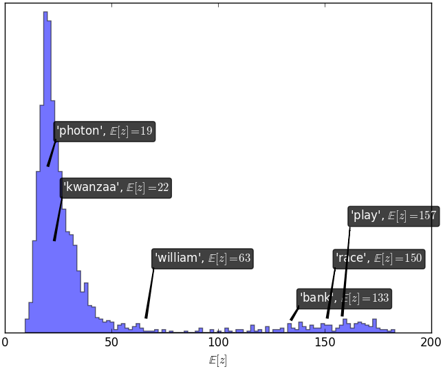
(a) Histogram of the expected dimensionalities.

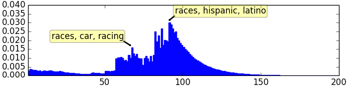
(b) $p(z|w=\text{`race'})$

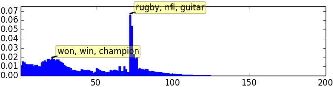
(c) $p(z|w=\text{`player'})$

Figure 1: Subfigure (a) shows results for semantic similarity tasks. The Spearman’s rank correlation between model and human scores are calculated for the WordSim-353 and MEN datasets. Subfigure (b) shows a histogram of the expected vector dimensionalities after training SD-CBOW. Subfigures (c) and (d) show the distribution over dimensionalities SD-SG learned for the words race and player.

4 Related Work

As mentioned in the Introduction, we are aware of no previous work that defines embedding dimensionality as a random variable whose distribution is learned from data. Yet, there is much existing work on increasing the flexibility of embeddings via auxiliary parameters. For instance, Vilnis & McCallum (2015) represent each word with a multivariate Gaussian distribution. The Gaussian embedding’s mean parameter serves much like a traditional vector representation, and the method’s novelty arises from the covariance parameter’s ability to capture word specificity (Vilnis and McCallum, 2015). Other related work proposes using multiple embeddings per word in order to handle polysemy and homonymy Huang et al. (2012); Reisinger and Mooney (2010); Neelakantan et al. (2014); Tian et al. (2014); Bartunov et al. (2016). Bartunov et al. (2016)’s AdaGram model is closest in spirit to SD-SG and SD-CBOW in that it uses the Dirichlet Process to learn an unconstrained, data-dependent number of embeddings for each word. Yet, in contrast to SD-SG/-CBOW, the dimensionality of each embedding is still user-specified.

5 Evaluation

We evaluate SD-SG and SD-CBOW quantitatively and qualitatively against original SG and CBOW. For all experiments, models were trained on a one billion word subset of Wikipedia (6/29/08 snapshot). The same learning rate ($\alpha=0.05$ for CBOW, $\alpha=0.025$ for SG), number of negative samples (5), context window size (6), and number of training epochs (1) were used for all models. SD-SG and SD-CBOW were initialized to ten dimensions.

Quantitative Evaluation. We test each model’s ability to rank word pairs according to their semantic similarity, a task commonly used to gauge the quality of WEs. We evaluate our embeddings on two standard test sets: WordSim353 (Finkelstein et al., 2001) and MEN (Bruni et al., 2014). As is typical for evaluation, we measure the Spearman’s rank correlation between the similarity scores produced by the model and those produced by humans. The correlations for all models are reported in Subtable (a) of Figure 1. We see that the SD-SG and SD-CBOW perform better than their 50 dimensional counterparts but worse than their 200 dimensional counterparts. All scores are relatively competitive though, separated by no more than $0.1$.

Qualitative Evaluation. Observing that the SD-SG and SD-CBOW models perform comparatively to finite versions somewhere between 50 and 200 dimensions, we qualitatively examine their distributions over vector dimensionalities. Subfigure (b) of Figure 1 shows a histogram of the expected dimensionality—i.e. $\mathbb{E}_{z|w,c}[z]$—of each vector after training the SD-CBOW model. As expected, the distribution is long-tailed, and vague words occupy the tail while specific words are found in the head. As shown by the annotations, the word photon has an expected dimensionality of 19 while the homograph race has 150. Note that expected dimensionality correlates with word frequency—due to the fact that multi-sense words, by definition, can be used more frequently—but does not follow it strictly. For instance, the word william is the 482nd most frequently occurring word in the corpus but has an expected length of 62, which is closer to the lengths of much rarer words (around 20-40 dimensions) than to similarly frequent words.

In subfigures (c) and (d) of Figure 1, we plot the quantity $p(z|w)$ for two homographs, race (c) and player (d), as learned by SD-SG, in order to examine if their multiple meanings are conspicuous in their distribution over dimensionalities. For race, we see that the distribution does indeed have at least two modes: the first at around 70 dimensions represents car racing, as determined by computing nearest neighbors with that dimension as a cutoff, while the second at around 100 dimensions encodes the anthropological meaning.

6 Conclusions

We propose modest modifications to SG and CBOW that allow embedding dimensionality to be learned from data in a probabilistically principled way. Our models preserve performance on semantic similarity tasks while providing a view–via the distribution $p(z|w,c)$–into how embeddings utilize their parameters and distribute semantic information.

Appendix

A Finite Partition Function

Stochastic Dimensionality Skip-Gram’s partition function, containing a sum over all countably infinite values of $z$, would seem to be divergent and thus incomputable. However, it is not, due to two key properties first proposed by Côté and Larochelle (2016) to define a Restricted Boltzmann Machine with an infinite number of hidden units (iRBM). They are:

1. Sparsity penalty: The $L2$ penalty in $E(\mathbf{w}_{i},\mathbf{c}_{k},z)$ (i.e. the $w_{i,j}^{2}$ and $c_{k,j}^{2}$ terms) ensures the word and context vectors must have a finite two-norm under iterative gradient-based optimization with a finite initial condition. In other words, no proper optimization method could converge to the infinite solution if all $\mathbf{w}$ and $\mathbf{c}$ vectors are initialized to have a finite number of non-zero elements (Côté and Larochelle, 2016).

2. Per-dimension constant penalty: The energy function’s $z\log a$ term results in dimensions greater than $l$ becoming a convergent geometric series. This is discussed further below.

With those two properties in mind, consider the conditional distribution of $z$ given an input and context word:

$$p(z|w,c)=\frac{e^{-E(\mathbf{w},\mathbf{c},z)}}{\sum_{z^{\prime}=1}^{\infty}e^{-E(\mathbf{w},\mathbf{c},z^{\prime})}}.$$ (7)

Again, the denominator looks problematic due to the infinite sum, but notice the following:

$$\begin{split}Z_{z}&=\sum_{z^{\prime}=1}^{l}e^{-E(\mathbf{w},\mathbf{c},z^{\prime})}+\sum_{z^{\prime}=l+1}^{\infty}e^{-E(\mathbf{w},\mathbf{c},z^{\prime})}\\ &=\sum_{z^{\prime}=1}^{l}e^{-E(\mathbf{w},\mathbf{c},z^{\prime})}+e^{-E(\mathbf{w},\mathbf{c},l)}\sum_{z^{\prime}=0}^{\infty}\frac{1}{a^{z^{\prime}}}\\ &=\sum_{z^{\prime}=1}^{l}e^{-E(\mathbf{w},\mathbf{c},z^{\prime})}+\frac{a}{a-1}e^{-E(\mathbf{w},\mathbf{c},l)}.\end{split}$$ (8)

The sparsity penalty allows the sum to be split as it is in step #2 into a finite term ($\sum_{z^{\prime}=1}^{l}e^{-E(\mathbf{w},\mathbf{c},z^{\prime})}$) and an infinite sum ($\sum_{z^{\prime}=l+1}^{\infty}e^{-E(\mathbf{w},\mathbf{c},z^{\prime})}$) at an index $l$ such that $w_{i,j}=c_{k,j}=0$ $\ \forall j>l$. After $e^{-E(\mathbf{w},\mathbf{c},l)}$ is factored out of the second term, all remaining $w_{i,j}$ and $c_{k,j}$ terms are zero. A few steps of algebra then reveal the presence of a convergent geometric series. Intuitively, we can think of the second term, $\frac{a}{a-1}e^{-E(\mathbf{w},\mathbf{c},l)}$, as quantifying the data’s need to expand the model’s capacity given $w$ and $c$.

References

- Bartunov et al. (2016) Sergey Bartunov, Dmitry Kondrashkin, Anton Osokin, and Dmitry Vetrov. 2016. Breaking sticks and ambiguities with adaptive skip-gram. International Conference on Artificial Intelligence and Statistics .
- Bengio et al. (2003) Yoshua Bengio, Réjean Ducharme, Pascal Vincent, and Christian Janvin. 2003. A neural probabilistic language model. The Journal of Machine Learning Research 3:1137–1155.
- Bruni et al. (2014) Elia Bruni, Nam Khanh Tran, and Marco Baroni. 2014. Multimodal distributional semantics. J. Artif. Int. Res. 49(1):1–47.
- Côté and Larochelle (2016) Marc-Alexandre Côté and Hugo Larochelle. 2016. An infinite restricted boltzmann machine. Neural computation .
- Finkelstein et al. (2001) Lev Finkelstein, Evgeniy Gabrilovich, Yossi Matias, Ehud Rivlin, Zach Solan, Gadi Wolfman, and Eytan Ruppin. 2001. Placing search in context: The concept revisited. In Proceedings of the 10th International Conference on World Wide Web. WWW ’01, pages 406–414.
- Huang et al. (2012) Eric H. Huang, Richard Socher, Christopher D. Manning, and Andrew Y. Ng. 2012. Improving word representations via global context and multiple word prototypes. In Annual Meeting of the Association for Computational Linguistics (ACL).
- Mikolov et al. (2013) Tomas Mikolov, Ilya Sutskever, Kai Chen, Greg S Corrado, and Jeff Dean. 2013. Distributed representations of words and phrases and their compositionality. In Advances in neural information processing systems. pages 3111–3119.
- Mnih and Hinton (2009) Andriy Mnih and Geoffrey E Hinton. 2009. A scalable hierarchical distributed language model. In Advances in neural information processing systems. pages 1081–1088.
- Neelakantan et al. (2014) Arvind Neelakantan, Jeevan Shankar, Alexandre Passos, and Andrew McCallum. 2014. Efficient non-parametric estimation of multiple embeddings per word in vector space. Conference on Empirical Methods in Natural Language Processing .
- Reisinger and Mooney (2010) Joseph Reisinger and Raymond J Mooney. 2010. Multi-prototype vector-space models of word meaning. In Human Language Technologies: The 2010 Annual Conference of the North American Chapter of the Association for Computational Linguistics. Association for Computational Linguistics, pages 109–117.
- Tian et al. (2014) Fei Tian, Hanjun Dai, Jiang Bian, Bin Gao, Rui Zhang, Enhong Chen, and Tie-Yan Liu. 2014. A probabilistic model for learning multi-prototype word embeddings. In Proceedings of COLING. pages 151–160.
- Turian et al. (2010) Joseph Turian, Lev Ratinov, and Yoshua Bengio. 2010. Word representations: a simple and general method for semi-supervised learning. In Proceedings of the 48th annual meeting of the association for computational linguistics. Association for Computational Linguistics, pages 384–394.
- Vilnis and McCallum (2015) Luke Vilnis and Andrew McCallum. 2015. Word representations via gaussian embedding. International Conference on Learning Representations .