Probabilistic Segmentation via Total Variation Regularization

Abstract

We present a convex approach to probabilistic segmentation and modeling of time series data. Our approach builds upon recent advances in multivariate total variation regularization, and seeks to learn a separate set of parameters for the distribution over the observations at each time point, but with an additional penalty that encourages the parameters to remain constant over time. We propose efficient optimization methods for solving the resulting (large) optimization problems, and a two-stage procedure for estimating recurring clusters under such models, based upon kernel density estimation. Finally, we show on a number of real-world segmentation tasks, the resulting methods often perform as well or better than existing latent variable models, while being substantially easier to train.

1 Introduction

In this paper, we consider the tasks of time series segmentation and modeling. Formally, suppose that we observe a sequence of $T$ input/output pairs, represented as

$$(x_{1},y_{1}),(x_{2},y_{2}),\ldots,(x_{T},y_{T})$$ (1)

for $x_{t}\in\mathbb{R}^{n}$ (which can even include functions of past outputs of the time series to capture scenarios such as autoregressive models) and $y_{t}\in\mathbb{R}^{p}$ (though we can also consider other possible forms of the output vector, such as categorical variables). Our goal is twofold: 1) to segment the time series into (potentially non-contiguous) partitions $x_{\mathcal{I}_{1}},\ldots,x_{\mathcal{I}_{k}}$, such that all the time points within each partition can be modeled via a single probabilistic model $p(y_{t}|x_{t};\theta_{i}),\;\;\forall t\in\mathcal{I}_{i}$, parameterized by $\theta_{i}\in\mathbb{R}^{d}$; and 2) to determine the parameter,s $\theta_{i}$, of each different segment. This is an extremely general problem formulation and captures many of the aims of time series latent variable models like hidden Markov models and their many extensions [14], multiple change-point detection methods [2], and switched dynamical systems [17].

A common approach to such tasks is what we generically refer to as a latent state mixture model, with an illustrative example shown in Figure 1 (left). In such models, we associate with each time a discrete latent state $z_{t}\in\{1,\ldots,k\}$ that “selects” parameters to use for modeling the conditional distribution $p(y_{t}|x_{t},z_{t})=p(y_{t}|x_{y};\theta_{z_{t}})$. Under such a model, the segmentation and modeling challenges above can be addressed respectively by e.g., 1) computing the most likely sequence of latent states; and 2) jointly inferring the distribution over hidden states and model parameters through the classical EM algorithm. Though such models are very powerful, the fact that the EM algorithm can be highly susceptible to local optima often makes learning such models difficult, especially for complex distributions with many parameters. Furthermore, although the model over the latent variables, $p(z_{t+1}|z_{t};A)$ can capture complex dynamics in the system, in practice a primary characteristic that these models must capture is simply a “stickiness” property: the fact that a system in state $z_{t}$ tends to stay in this state with relatively high probability; indeed, including such properties in latent variable models has been crucial to obtaining good performance [8].

In this work, we propose to capture very similar behavior, but in a fully convex probabilistic framework. In particular, we directly associate with each time point a separate set of parameters, $\theta_{t}$, but then encourage the parameters to remain constant over time by penalizing the $\ell_{2}$ norm of the difference between successive parameters. As is well-known from the group lasso setting [21], a penalty on the $\ell_{2}$ norm will encourage group sparseness in the differences, i.e., a piecewise-constant sequence of parameters; a graphical representation of this approach is show in Figure 1. Formally, we jointly segment and model the system by solving the (convex) optimization problem

$$\operatorname*{\mathrm{minimize}}_{\theta_{1},\ldots,\theta_{T}}\;\;-\sum_{t=1}^{T}\log p(y_{t}|x_{t};\theta_{t})+\lambda\sum_{t=1}^{T-1}\|\theta_{t+1}-\theta_{t}\|_{2}.$$ (2)

This penalty function on $\theta$ is sometimes referred to as the group fused lasso [1, 3] or the multivariate total variation penalty, but the key of our approach is to apply such penalties to the underlying parameters of the probability distribution rather than to the output signal itself. The resulting model generalizes several existing methods from the literature, including the standard group fused lasso itself [3], time-varying linear regression [12] and auto-regressive modeling [13], and $\ell_{1}$ mean and variance filtering [18].

Although the proposed approach is conceptually simple, there are a number of elements needed to make this approach practical; together, these make up the majority of our contribution in this work. First, the optimization problem (2) is challenging: it involves a $kT$ dimensional optimization variable, potentially non-quadratic loss functions, a non-smooth $\ell_{2}$ norm penalty, and achieving exact sparseness in these differences is crucial given that we want to use the method to split the time series into distinct segments. Second, a major advantage of latent variable models is that they can capture disjoint segments, where the underlying parameters change and return to previous values; this structure is inherently missed by the total variation penalties, as there is no innate mechanism by which we can “return” to previous parameter values. Instead, we propose to capture much of this same behavior via a two-pass algorithm that clusters the parameters themselves using kernel density estimation. Finally, the main message of this paper is an empirical one, that the convex framework (2) can perform as well, in practice, as much more complex latent variable models, while simultaneously being much faster and easier to optimize. Thus, we present empirical results on three real-world domains studied in the latent variable modeling literature: segmenting honey bee motion, detecting and modeling device energy consumption in a home, and segmenting motion capture data. Together, these illustrate the wide applicability of the proposed approach.

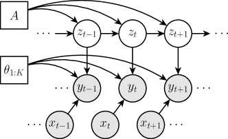
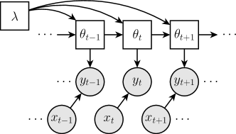
Figure 1: A generic latent variable time series model (left) and our convex framework for segmentation and modeling (right).

2 Efficient ADMM optimization method with fast Newton subroutines

In this section, we develop fast algorithms for solving the probabilistic segmentation problem (2) with different probabilistic models $p(y_{t}|x_{t};\theta_{t})$, a necessary step for applying the model to real data sets. Although the problem is convex, optimization is complicated by the non-smooth nature of the total variation norm (i.e. exactly the structure that promotes sparsity in the change points which we desire) and the composite objective incorporating a probability distribution with a possibly different set of parameters at each time point. The result is a difficult-to-solve optimization problem, and we found that off-the-shelf solvers performed poorly on even moderately sized examples. Our approach to optimization decomposes the objective into many smaller subproblems using the alternating direction methods of multipliers (ADMM) [4]—iterating between solving the subproblems and taking a gradient step in the dual.

Omitting details for the sake of brevity (the derivations here are straightforward and for a thorough description of ADMM including complete description of the algorithm, we refer readers to [4] and a similar form form of ADMM, though just for quadratic loss, is also described in [19]), for problems of the form (2), the algorithm iteratively performs the following updates starting at some initial $\theta_{1:T}^{0}$, $z_{1:T}^{0}$, and $u_{1:T}^{0}$:

$$\begin{split}\theta^{k+1}_{t}&\leftarrow\operatorname*{\mathrm{argmin}}_{\theta_{t}}\;\;-\log p(y_{t}|x_{t};\theta_{t})+\frac{\rho}{2}\|\theta_{t}-z^{k}_{t}+u^{k}_{t}\|_{2}^{2},\;\;\forall t=1,\ldots,T\\ z^{k+1}_{1:T}&\leftarrow\operatorname*{\mathrm{argmin}}_{z_{1:T}}\;\;\sum_{t=1}^{T-1}\|z_{t}-z_{t+1}\|_{2}+\frac{\rho}{2}\sum_{t=1}^{T}\|x^{k+1}_{t}-z_{t}+u^{k}_{t}\|_{2}^{2}\\ u^{k+1}_{t}&\leftarrow u^{k}_{t}+x^{k+1}_{t}-z^{k+1}_{t},\;\;\forall t=1,\ldots,T.\end{split}$$ (3)

ADMM is particularly appealing for such problems because the $z$ update here is precisely a group fused lasso, a problem for which efficient second-order methods exist [19], and because the $\theta_{t}$ updates are separate, which allows the method to be trivially parallelized. In addition, the proposed ADMM approach is appealing because it is extensible—for example, we could encode additional structure in the problem by penalizing the trace norm [15] of $[\theta_{1},\ldots,\theta_{T}]$, an extension that is straightforward requiring only minor modifications to the algorithm and the implementation of the proximal operator for this new penalty (in this case, thresholding on singular values).

While fast algorithms exist for the total variation norm, the novel element required for our problem is efficient implementation of the proximal operators for the log-loss term, that is, the $\theta$ updates in (3). In particular (observing that the this term separates over time points, we drop the subscript $t$) we derive efficient implementations for the subproblems

$$\operatorname*{\mathrm{minimize}}_{\theta}-\log p(y|x;\theta)+\frac{\rho}{2}\|\theta-\theta_{0}\|_{2}^{2}.$$ (4)

Note that since our framework allows for the possibility of different parameters at each time point, in each iteration of ADMM we must solve this problem $T$ times resulting in different estimates for $\theta_{t}$, a setting somewhat different than standard maximum likelihood estimation in which we estimate one set of parameters for many data points. Furthermore, as we highlight in the sequel, minimizing the log-loss term over only a single observation gives rise to additional structure which we can exploit. Next, we consider fast updates for the cause of a multivariate conditional Gaussian (with unknown covariance/precision matrix), a natural distribution for our model. The models are of course also extensible to other probability models such as the softmax model for discrete outputs, and the resulting method is very similar to that presented below. Code for the full algorithm will be included with the final version of the paper.

2.1 Gaussian model

Suppose we have a continuous output variable $y\in\mathbb{R}^{p}$ and we model $y|x$ as

$$p(y|x;\Lambda,\Theta)=\frac{1}{Z(x)}\exp\left(-\frac{1}{2}y^{T}\Lambda y-x^{T}\Theta y\right)$$ (5)

with parameters $\Lambda\in\mathbb{R}^{p\times p}$ and $\Theta\in\mathbb{R}^{n\times p}$; note that under this model, $\Theta$ and $\Lambda$ take the place of $\theta$ with $\theta=[\operatorname*{\mathrm{vec}}(\Lambda)^{T},\operatorname*{\mathrm{vec}}(\Theta)^{T}]^{T}$ and for the rest of this section we simply consider the parameters to be $\Lambda$ and $\Theta$ for ease of notation. This model is equivalent to a multivariate Gaussian with $y|x\sim\mathcal{N}(-\Lambda^{-1}\Theta^{T}x,\Lambda^{-1})$ but this particular parameterization with the scaled mean parameter is attractive as it admits a convex regularized maximum likelihood estimation problem:

$$\operatorname*{\mathrm{minimize}}_{\Lambda,\Theta}-\log\det\Lambda+y^{T}\Lambda y+x^{T}\Theta^{T}\Lambda^{-1}\Theta x+2y^{T}\Theta x+\frac{\rho}{2}\left(\|\Lambda-\Lambda_{0}\|_{F}^{2}+\|\Theta-\Theta_{0}\|_{F}^{2}\right).$$ (6)

This problem is convex and without the addition of the augmented Lagrangian terms can be solved in closed form; however, with those terms no such closed form exists and thus our approach is to develop a second-order Newton method. We start by taking the gradient

$$\begin{split}\nabla_{\Lambda}&=-\Lambda^{-1}+yy^{T}-\Lambda^{-1}\Theta^{T}xx^{T}\Theta\Lambda^{-1}+\rho(\Lambda-\Lambda_{0})\\ \nabla_{\Theta}&=2xx^{T}\Theta\Lambda^{-1}+2xy^{T}+\rho(\Theta-\Theta_{0})\end{split}$$ (7)

and we solve for the Newton direction, parameterized by $(U,V)$ where $U$ represents the change in $\Lambda$ and $V$ in $\Theta$, by considering the system of equations

$$\begin{split}\Lambda^{-1}U\Lambda^{-1}+\Lambda^{-1}\Theta^{T}xx^{T}\Theta\Lambda^{-1}U\Lambda^{-1}+\Lambda^{-1}U\Lambda^{-1}\Theta^{T}xx^{T}\Theta\Lambda^{-1}\\ -\Lambda^{-1}V^{T}xx^{T}\Theta\Lambda^{-1}-\Lambda^{-1}\Theta^{T}xx^{T}V\Lambda^{-1}+\rho U&=\nabla_{\Lambda}\\ 2xx^{T}V\Lambda^{-1}-2xx^{T}\Theta\Lambda^{-1}U\Lambda^{-1}+\rho V&=\nabla_{\Theta}\end{split}$$ (8)

which is a Sylvester-like equation that we could solve using the identity $\operatorname*{\mathrm{vec}}(AXB)=(B^{T}\otimes A)\operatorname*{\mathrm{vec}}(A)$ where $\otimes$ denotes the Kronecker product.

However, naively employing this approach requires inverting a $p(n+p)\times p(n+p)$ matrix and thus is not computationally tractable for reasonably sized problems. Instead, we simplify the system of equations analytically so that solving for the Newton direction requires only $O(p^{3})$ operations. We proceed by taking the eigendecomposition $\Lambda^{-1}=WSW^{T}$ and writing this system of equations as

$$\begin{split}S\tilde{U}S+S\tilde{\Theta}^{T}xx^{T}\tilde{\Theta}S\tilde{U}S+S\tilde{U}S\tilde{\Theta}^{T}xx^{T}\tilde{\Theta}S\\ -S\tilde{V}^{T}xx^{T}\tilde{\Theta}S-S\tilde{\Theta}^{T}xx^{T}\tilde{V}S+\rho\tilde{U}&=W^{T}\nabla_{\Lambda}W\\ 2xx^{T}\tilde{V}S-2xx^{T}\tilde{\Theta}S\tilde{U}S+\rho\tilde{V}&=\nabla_{\Theta}W\end{split}$$ (9)

where $\tilde{U}=W^{T}UW$, $\tilde{V}=VW$ and $\tilde{\Theta}=\Theta W$. Now using the $\operatorname*{\mathrm{vec}}$ operator we have

$$\left[\begin{array}[]{cc}S\otimes S+S\otimes aa^{T}+aa^{T}\otimes S+\rho I&S\otimes ax^{T}+(S\otimes ax^{T})K_{np}\\ S\otimes xa^{T}+K_{pn}(xa^{T}\otimes S)&2S\otimes xx^{T}+\rho I\end{array}\right]\left[\begin{array}[]{cc}\operatorname*{\mathrm{vec}}\tilde{U}\\ \operatorname*{\mathrm{vec}}\tilde{V}\end{array}\right]=\left[\begin{array}[]{cc}\operatorname*{\mathrm{vec}}{W^{T}\nabla_{\Lambda}W}\\ \operatorname*{\mathrm{vec}}\nabla_{\Theta}W\end{array}\right]$$ (10)

where $a=-S\tilde{\Theta}^{T}x$ and $K_{np}$ is the commutation matrix (see e.g. [10]). Although the matrix on the LHS of this linear system is large, it is highly structured; specifically it can be factorized into diagonal and low rank components, written as $D+AA^{T}$ with

$$D=\left[\begin{array}[]{cc}S\otimes S+\rho I&0\\ 0&\rho I\end{array}\right] A=\left[\begin{array}[]{cc}S^{1/2}\otimes a&a\otimes S^{1/2}\\ S^{1/2}\otimes x&S^{1/2}\otimes x\end{array}\right].$$ (15)

Next, using the matrix inversion lemma we have

$$(D+AA^{T})^{-1}=D^{-1}-D^{-1}A(I+A^{T}D^{-1}A)^{-1}A^{T}D^{-1}$$ (16)

and after a bit of algebra, we observe that

$$(I+A^{T}D^{-1}A)=\left[\begin{array}[]{cc}X+C_{1}&X+C_{2}\\ X+C_{2}&X+C_{1}\end{array}\right]$$ (17)

where

$$X=\frac{1}{\rho}(x^{T}x)S, C_{1}=\operatorname*{\mathrm{diag}}\left(\frac{(a\circ a)s^{T}}{ss^{T}+\rho}1\right), C_{2}=\frac{S^{1/2}aa^{T}S^{1/2}}{ss^{T}+\rho}.$$ (18)

Using this form, we are able to compute each term in the Newton direction $(D+AA^{T})^{-1}\operatorname*{\mathrm{vec}}(G)$ where $G$ is the RHS of the equation from (10) without ever forming the Kronecker products explicitly resulting in a computation complexity of $O(p^{3})$, the cost to invert (17).

3 Segment clustering via kernel density estimation

As mentioned above, a notable disadvantage our proposed convex segmentation methods is that, unlike latent variable models, there is no inherent notion of parameters being tied across disjoint segments of the time series. Indeed, the effect of the above segmentation model will be to determine the best single model for each segment individually (modulo the regularization penalties). Although we observe that, in real-world settings, this does not appear to be as large a problem as might be imagined for learning the individual model parameters themselves (the “stickiness” component mentioned above typically means that there is enough data per segment to learn good models), it is a substantial concern if the overall goal is to make joint inferences about the nature of related segments in the same time series or across multiple time series. To this end, we advocate for a two-stage alternative to the latent variable model: in the first stage,we compute the convex segmentation as above and in the second stage, we cluster the segments directly in parameter space, via kernel density estimation.

While there are many methods to cluster points in Euclidean space, density clustering using the kernel estimator is appealing as identifying modes in the distribution over the parameter space fits well with our probabilistic model. The intuitive idea is that given the true probability distribution over the parameter space $p$ and a point $\theta\in\mathbb{R}^{d}$, we define the cluster for $\theta$ to be the mode found by following the gradient $\nabla p(\theta)$. In practice, since we do not know the true underlying distribution, we replace $p$ with $\hat{p}_{h}$, the kernel density estimator constructed with bandwidth $h$

$$\hat{p}_{h}(\theta)=\frac{1}{T}\sum_{t=1}^{T}\frac{1}{h^{d}}K\left(\frac{\|\theta-\theta_{t}\|}{h}\right)$$ (19)

where $K$ is a smooth, symmetric kernel. The standard kernel choice (which we use) is the Gaussian kernel; in this case, it is known that the number of modes of $\hat{p}_{h}$ is a nonincreasing function of $h$ [16] and thus the clustering is well-behaved. Furthermore, given this property, in practice we typically fix the number of clusters based on the application and choose $h$ such that kernel density clustering results in the desired number of modes. However, we note that there are several possibilities for a more nuanced selection of the bandwidth—for example, we could select $h$ based on the terms of the objective function or the difference in norms between adjacent segments.

4 Experimental results

In this section, we evaluate the proposed method on several applications, some of which were previously considered in the context of parametric and nonparametric latent variable models using Bayesian inference [6, 7, 11, 20]. In these applications, we typically demonstrate equal or better performance with a substantially different approach—unlike the latent variables models, our method is fully convex and thus not subject to local optima. Following the direction of previous work, we treat these tasks as unsupervised with the parameter $\lambda$ controlling the trade-off between the complexity of the model (number of change points) and the data fit. In addition to considering our probabilistic method (“TV Gaussian”), we also consider the previously proposed linear regression model [12] (“TV LR”) in which case the log-loss term simply becomes the least squares penalty.

Table 1: Performance on dancing honey bees data set.

	1	2	3	4	5	6	Average
HDP-VAR(1)-HMM unsupervised	46.5	44.1	45.6	83.2	93.2	88.7	66.9
HDP-VAR(1)-HMM partially supervised	65.9	88.5	79.2	86.9	92.3	89.1	83.7
SLDS DD-MCMC	74.0	86.1	81.3	93.4	90.2	90.4	85.9
PS-SLDS DD-MCMC	75.9	92.4	83.1	93.4	90.4	91.0	87.7
TV Linear regression	54.4	47.7	79.6	78.8	76.1	75.5	68.9
TV Gaussian	82.2	83.3	76.1	91.1	93.1	93.1	86.5

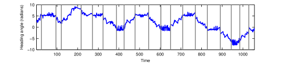
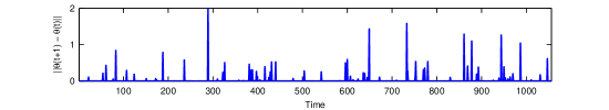
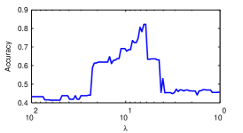
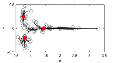
Figure 2: Segmentation results for honey bee sequence 1 with top plot showing the observed heading angle of the bee along with the (unobserved) segmentation provided by human experts. In middle, we show the segmentation provided by the best choice of $\lambda$ and on bottom left the comparison of performance vs. $\lambda$. On bottom right, the parameters for each segment (gray circles) are clustered using kernel density estimation to identify three modes (red circles).

Dancing honey bees. Our first data set involves tracking honey bees from video, a task that was first considered in [11] and subsequently studied by [20, 6]. The data includes the output of a vision system which identifies the bees position and heading angle over time and the task is to segment these observed values into three distinct actions: turn left, turn right and “waggle”—characterized by rapid back and forth movement. It is known that these actions are used by the bees to communicate about food sources, and for the 6 sequences provided we also have a ground truth labeling of actions by human experts. In Figure 2 (top) we show the angle variable along with labels showing behavior changes; as can be seen from the graph, we found that the change in angle to be highly indicative of the bees behavior, to the extent that we model this time series ignoring the other data. Specifically we take first order differences $y_{t}=\phi_{t+1}-\phi_{t}$ and represent this sequence probabilistically as $y_{t}\sim\mathcal{N}(\mu_{t},\sigma^{2}_{t})$, expecting that both the mean and variance to change based on the bee’s action.

In Table 1 we compare the accuracy of our segmentation using the best setting of $\lambda$ to that of previous work on this data set [11, 6]. Although this is an optimistic comparison, we observe that our method is not especially sensitive to $\lambda$ as can be seen in Figure 2 (bottom left); in particular, while the performance is particularly good for the best $\lambda$, there is a wide range in which the model performs as well or better than the other methods. It should also be noted that with the exception of “HDP-VAR(1)-HMM unsupervised” all of the considered approaches include some level of supervision (e.g. first training on the other 5 sequences) while our method is fully unsupervised with only a single tuning parameter. Next, considering the distribution of the parameters using kernel density estimation, we see in Figure 2 (bottom right) that our method indeed identifies the 3 modes of the distribution corresponding to labeled actions: turning left/right correspond to positive/negative mean while waggle has zero mean but significantly larger variance. The change in variance offers one intuitive explanation as to why the probabilistic model outperforms linear regression on this data set since the latter does not model this behavior.

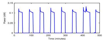
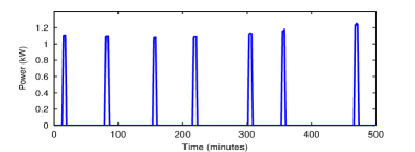
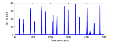
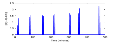
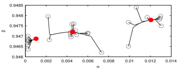
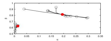
Figure 3: Segmentation results for power traces from the Pecan street data set with refrigerator on left and A/C on right. We model each device with an AR(1) process parameterized as $y_{t}=\alpha_{t}+\beta_{t}y_{t-1}$ and in the middle row show a particular segmentation for each device using $\lambda=0.1$ and $1$, respectively. The bottom row shows the result of kernel density estimation for clustering the parameter space, identifying 2 modes (off/on) for the A/C and 3 modes for the refrigerator—the third capturing the initial spike when the refrigerator switches on.

Modeling sources of energy consumption. In our next example, we consider the task of modeling energy consumed by household appliances using data from Pecan Street, Inc. (http://www.pecanstreet.org/) collected with current sensors installed at the circuit level inside the home. In this data set each device has a unique energy profile and our goal is to build accurate models which can be used to understand energy consumption in order to improve energy efficiency. In Figure 3 (top) we show typical power traces for two such devices, a refrigerator and A/C unit—these devices that are characterized by a small number of states and and their energy usage demonstrates strong persistence between being on/off which we capture with an AR(1) model parameterized by $y_{t}=\alpha_{t}+\beta_{t}y_{t-1}$. Empirically (as in the previous example) we found that the probabilistic approach improved significantly upon the simpler linear regression model which typically did not produce segments corresponding to logical device states (the on state was often over-segmented). In contrast, Figure 3 (bottom) shows the estimated modes from probabilistic segmentation which correspond to an off state, on state, and in the case of the refrigerator, a state representing the initial spike in energy consumed when the device transitions from off to on.

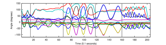
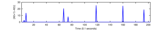
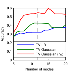
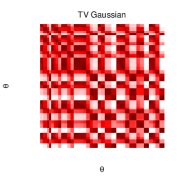
Figure 4: Segmentation results on motion capture with input data of 12 joint angles measured at 10Hz and manual segmentation on top; in middle, the segmentation from the AR(2) Gaussian model plus iterative reweighting. On bottom, we compare accuracy on identifying actions (segmentation plus clustering) with the reweighted Gaussian model performing the best. We examine this behavior on bottom middle/right, by reordering $\theta_{1},\ldots,\theta_{T}$ so that identical actions are adjacent and consider distance between pairs $(\theta_{t},\theta_{t^{\prime}})$ with dark signifying closer. Comparing middle (non-reweighted) vs. right (reweighted), the evident block structure indicates that parameters for the same action are relatively closer after reweighting (presumably) allows for better parameter estimation.

Motion capture. In our final example we consider segmenting motion capture data, a task first proposed in [7] in conjunction with a hierarchical nonparametric Bayesian model specifically designed to jointly model behavior across subjects. We attempt to replicate that experimental setup here which includes sub-selecting from 62 available measurements a representative set of 12 angles characterizing the behavior of the subject and manually labeling the sequences with one of 12 actions. A typical sequence is shown in Figure 4 (top), which (after normalization) we take as the output variables $y_{t}\in\mathbb{R}^{12}$. As the signal shows not only persistence but also clear periodic structure, we model this as an AR(2) process resulting in $x_{t}\in\mathbb{R}^{25}$ and a parameter space with much higher dimension that in previous examples (in the Gaussian model, $\Lambda_{t}\in\mathbb{R}^{12\times 12}$ and $\Theta_{t}\in\mathbb{R}^{25\times 12}$).

First, in Figure 4 (middle) we have an accurate segmentation provided by the Gaussian model with the additional step of a few iterations of iterative reweighting [5], an extension to the algorithm that previous authors have suggested in the case of linear regression [13]. We found that while all methods considered on this data set performed well on segmentation, the addition of the reweighting step improved parameter estimation significantly resulting in the better performance shown in Figure 4 (bottom left); here the comparison depends on both accurate segmentation and parameter estimation in order for density-based clustering to identifying similar segments which is required to do well on this task.

The intuition behind the improvement from reweighting is shown in Figure 4 (bottom right) which compares the distance of the parameters after segmentation for the Gaussian model and the Gaussian model plus reweighting—we see that when the parameters are allowed to vary more significantly between segments (as a consequence of reweighting), the parameters corresponding to the same action remains close relative to the parameters for different actions. This is likely due to better parameter estimation on the individual segments from reducing the bias from total variation regularization. Overall, the reweighted Gaussian model achieves accuracy of around 60% which is comparable to most previous results from [7] but somewhat worse than the best model which is specifically designed for this task and benefits from highly structured prior information.

5 Conclusions and future work

At a basic level, the techniques proposed in this paper center around finding a convex (and hence, local-optima-free) approach to modeling time series data in a manner that naturally segments the data into different probabilistic models. While the proposed method works well in many settings, numerous extensions are possible in the overall framework. For instance, we can consider imposing additional regularization on the joint space of parameters to enforce further structure; we can generalize the getting to many other possible loss functions; we can generalize the total variation penalty to the more general $\ell_{1}$ trend filtering setting [9], to capture linear or higher order smooth segments in parameter space; and we can extend the total variation penalty non-adjacent time points, potentially directly allowing for segmentation across non-contiguous regions. Further, we can explore extensions to kernel density estimation in the parameter space that explicitly model the evolution of these parameters, allowing us to build a full generative model rather than just finding modes as we do now. Together, we believe that this combination of approaches can lead to time series methods competitive with latent variable models in terms of their flexibility and representational power, but which are substantially easier and more efficient to build and learn.

References

- [1] Carlos M Alaız, Álvaro Barbero, and José R Dorronsoro. Group fused lasso. Artificial Neural Networks and Machine Learning–ICANN 2013, page 66, 2013.
- [2] Michèle Basseville, Igor V Nikiforov, et al. Detection of abrupt changes: theory and application, volume 104. Prentice Hall Englewood Cliffs, 1993.
- [3] Kevin Bleakley and Jean-Philippe Vert. The group fused lasso for multiple change-point detection. arXiv preprint arXiv:1106.4199, 2011.
- [4] Stephen Boyd, Neal Parikh, Eric Chu, Borja Peleato, and Jonathan Eckstein. Distributed optimization and statistical learning via the alternating direction method of multipliers. Foundations and Trends® in Machine Learning, 3(1):1–122, 2011.
- [5] Emmanuel J Candes, Michael B Wakin, and Stephen P Boyd. Enhancing sparsity by reweighted ℓ 1 minimization. Journal of Fourier analysis and applications, 14(5-6):877–905, 2008.
- [6] Emily Fox, Erik B Sudderth, Michael I Jordan, and Alan Willsky. Bayesian nonparametric inference of switching dynamic linear models. Signal Processing, IEEE Transactions on, 59(4):1569–1585, 2011.
- [7] Emily B Fox, Michael C Hughes, Erik B Sudderth, and Michael I Jordan. Joint modeling of multiple time series via the beta process with application to motion capture segmentation. arXiv preprint arXiv:1308.4747, 2013.
- [8] Emily B Fox, Erik B Sudderth, Michael I Jordan, Alan S Willsky, et al. A sticky hdp-hmm with application to speaker diarization. The Annals of Applied Statistics, 5(2A):1020–1056, 2011.
- [9] Seung-Jean Kim, Kwangmoo Koh, Stephen Boyd, and Dimitry Gorinevsky. trend filtering. Siam Review, 51(2):339–360, 2009.
- [10] Jan R Magnus and Heinz Neudecker. Matrix differential calculus with applications in statistics and econometrics. 1988.
- [11] Sang Min Oh, James M Rehg, Tucker Balch, and Frank Dellaert. Learning and inferring motion patterns using parametric segmental switching linear dynamic systems. International Journal of Computer Vision, 77(1-3):103–124, 2008.
- [12] Henrik Ohlsson and Lennart Ljung. Identification of switched linear regression models using sum-of-norms regularization. Automatica, 49(4):1045–1050, 2013.
- [13] Henrik Ohlsson, Lennart Ljung, and Stephen Boyd. Segmentation of arx-models using sum-of-norms regularization. Automatica, 46(6):1107–1111, 2010.
- [14] Lawrence Rabiner. A tutorial on hidden markov models and selected applications in speech recognition. Proceedings of the IEEE, 77(2):257–286, 1989.
- [15] Benjamin Recht, Maryam Fazel, and Pablo A Parrilo. Guaranteed minimum-rank solutions of linear matrix equations via nuclear norm minimization. SIAM review, 52(3):471–501, 2010.
- [16] Bernard W Silverman. Using kernel density estimates to investigate multimodality. Journal of the Royal Statistical Society. Series B (Methodological), pages 97–99, 1981.
- [17] Zhendong Sun. Switched linear systems: Control and design. Springer, 2006.
- [18] Bo Wahlberg, Stephen Boyd, Mariette Annergren, and Yang Wang. An admm algorithm for a class of total variation regularized estimation problems. arXiv preprint arXiv:1203.1828, 2012.
- [19] Matt Wytock, Suvrit Sra, and J. Zico Kolter. Fast Newton methods for the group fused lasso. In Uncertainty in Artificial Intelligence, 2014.
- [20] Xiang Xuan and Kevin Murphy. Modeling changing dependency structure in multivariate time series. In Proceedings of the 24th international conference on Machine learning, pages 1055–1062. ACM, 2007.
- [21] Ming Yuan and Yi Lin. Model selection and estimation in regression with grouped variables. Journal of the Royal Statistical Society: Series B (Statistical Methodology), 68(1):49–67, 2006.