Imprints of relic gravitational waves on pulsar timing^∗

Abstract

Relic gravitational waves (RGWs) , a background originated during inflation, would give imprints on the pulsar timing residuals. This makes RGWs be one of important sources for detection using the method of pulsar timing. In this paper, we discuss the effects of RGWs on the single pulsar timing, and give quantitively the timing residuals caused by RGWs with different model parameters. In principle, if the RGWs are strong enough today, they can be detected by timing a single millisecond pulsar with high precision after the intrinsic red noise in pulsar timing residuals were understood, even though observing simultaneously multiple millisecond pulsars is a more powerful technique in extracting gravitational wave signals. We corrected the normalization of RGWs using observations of the cosmic microwave background (CMB), which leads to the amplitudes of RGWs being reduced by two orders of magnitude or so compared to our previous works. We made new constraints on RGWs using the recent observations from the Parkes Pulsar Timing Array, employing the tensor-to-scalar ratio $r=0.2$ due to the tensor-type polarization observations of CMB by BICEP2 as a referenced value even though it has been denied. Moreover, the constraints on RGWs from CMB and BBN (Big Bang nucleosynthesis) will also be discussed for comparison.

1 Introduction

A stochastic background of relic gravitational waves (RGWs) is predicted by the validities of both general relativity and quantum mechanics (Grishchuk 1975; Grishchuk 2001; Starobinsky 1979; Maggiore 2000; Zhang et al. 2005; Zhang et al. 2006; Miao & Zhang 2007; Giovannini 2010). It was originated from the quantum fluctuations during the inflationary stage. Hence, RGWs carry an unique information of the very early universe and serve as a probe into the universe much earlier than the cosmic microwave background (CMB) can do. As an advantage for detection, RGWs spread a very broad frequency band, $\sim 10^{-19}-10^{10}$ Hz, which make them be one of the major scientific targets of various types of gravitational wave (GW) detectors, such as the ground-based interferometers at $10^{2}-10^{3}$ Hz (The LIGO Scientific Collaboration & The Virgo Collaboration 2009; Willkeet al. 2002; Acernese 2005; Somiya 2012), the space-based interferometers at $10^{-4}-10^{-1}$ Hz ( Seto et al. 2001; Crowder & Cornish 2005; Cutler & Harms 2006; Kawamura et al. 2006; Amaro-Seoane et al. 2012), and high-frequency GW detectors around 100 MHz (Cruise 2000; Tong & Zhang 2008; Li et al. 2003; Li et al. 2008; Tong et al. 2008; Akutsu et al. 2008). For the very low frequency around $10^{-18}$ Hz, RGWs can be detected by the measuring the magnetic type of polarization of CMB (Zaldarriaga & Seljak 1997; Kaminonkowski et al. 1997), which has been a detecting goal of WMAP (Page et al. 2007; Komatsu et al. 2011; Hinshaw et al. 2013), Planck (Planck Collaboration 2014), and BICEP2 (Ade et al. 2014).

Another important tool to detect RGWs directly is pulsar timing. The existence of a stochastic gravitational wave (GW) background will make the times of arrival (TOA) of the pulses emitted from pulsars fluctuate. The fluctuations of TOA are implied in the pulsar timing residuals. If multiple millisecond pulsars are observed simultaneously, forming the pulsar timing arrays (PTAs) (Detweiler 1979; Romani & Taylor 1983; Hellings & Downs 1983; Kaspi et al. 1994), the GW signals can be extracted by correlating the timing residuals of each pair (Detweiler 1979; Jenet et al. 2005). PTAs respond to the frequency range of $10^{-9}-10^{-6}$ Hz, determined by the observational Characteristics. Currently, there are several such projects running, such as the Parkes Pulsar Timing Array (PPTA) (Hobbs 2008; Manchester 2013), European Pulsar Timing Array (EPTA) (van Haasteren et al. (2011)), the North American Nanohertz Observatory for Gravitational Waves (NANOGrav) (Demorest et al. 2013). The much more sensitive Five-hundred-meter Aperture Spherical Radio Telescope (FAST) (Nan 2011; Hobbs et al. 2014) and Square Kilometre Array (SKA) (Kramer et al. 2004; Janssen et al. 2015) are also under planning.

Even though there is no direct detection of RGWs so far, one can still give constraints on RGWs based on the current observations and some conceivable theories. These constraints could prevent us from choosing some unreasonable parameters of RGWs. At present, various constraints on GW background have been studied. The recent observations from Parkes Pulsar Timing Array (PPTA) gave an upper limit on the energy density spectrum $\Omega_{g}(f_{\rm PPTA})$ at $f_{\rm PPTA}=2.8$ nHz (Shannon et al. 2013). On the other hand, the physical processes happened in the early universe can also given constraints on RGWs. The successful Big Bang nucleosynthesis (BBN) puts a tight upper bound on the total energy fraction (Maggiore 2000) of GW background for frequencies $f>10^{-10}$ Hz (Allen & Romano 1999). The CMB and matter power spectra also give an upper limit of the total energy fraction of GWs for frequencies $f>10^{-15}$ Hz (Smith et al. 2006). Therefore, a successful model of RGWs should be compatible with the above constraints. The RGWs spectrum is, to a large extent, mainly described by the initial amplitude normalized by the tensor-to-scalar ratio $r$ (Boyle & Steinhardt 2008) and the inflation spectral index $\beta$ (Grishchuk 2001; Zhang et al. 2005; Miao & Zhang 2007; Tong & Zhang 2009). Here, we assume a zero running spectral index $\alpha_{t}$ (Tong & Zhang 2009), since it only affects the spectrum at high frequencies. Since $\beta$ describes directly the expansion behavior of inflation, the determination or constraint of $\beta$ would be powerful in discriminating inflationary models. The afore-mentioned bounds can be converted into the constraints on $\beta$ for a fixed $r$ (Tong & Zhang 2009; Zhang et al. 2010) and for a varying $r$ as a general analysis (Tong et al. 2014). The WMAP observations of the spectra of CMB anisotropies and polarization have yielded upper bounds on the ratio $r$ of RGWs for the fixed scalar index (Komatsu et al. 2011). Moreover, the recent observations of the polarizations of CMB by BICEP2 (Ade et al. 2014) gave a best estimation: $r=0.2$. Even though this result is disfavored now, we still use $r=0.2$ as a referenced value throughout this paper.

It is worth to point out that, we corrected the normalization of the amplitude of RGWs at a pivot $k_{0}$ by using the tensor-type power spectrum of CMB at the time of $k_{0}$ mode re-entering the Hubble horizon instead of that at the present time. This will reduce the amplitudes of RGWs for all the modes by two orders of magnitude or so compared to our previous works (Tong 2012; Tong et al. 2014). Hence, we will give new constraints on RGWs based on the theoretical RGWs and the updated observational data of PPTA. As a general discussion, we will not employ the quantum normalization (Grishchuk 2001; Tong et al. 2014) in this paper. Based on that, we will study how RGWs affect pulsar timing with different values of $\beta$ both in the time domain and the frequency domain. Moreover, we will quantitively calculated the corresponding pulsar timing residuals induced by RGWs for different $\beta$. Even though observing simultaneously multiple millisecond pulsars is a more powerful technique in extracting gravitational wave signals, in this paper we only discuss the effect of RGWs on the TOAs of an individual pulsar since it is the basement for gravitational wave detection by PTAs. In principle, one can also extract the signal of GWs from a single timing residuals with the assumption that the intrinsic red noises are understood. Thus, a comparison between the detecting sensitive curve determined by the ground clock and white-timing noise with the theoretical spectra of RGWs will be given.

Throughout this paper we the use units in which the light speed $c=1$.

2 Relic gravitational waves in the accelerating universe

In a spatially flat universe, the perturbed Friedmann-Robertson-Walker metric under the existence of the RGWs is

$$ds^{2}=a^{2}(\tau)[-d\tau^{2}+(\delta_{ij}+h_{ij})dx^{i}dx^{j}],$$ (1)

where $a(\tau)$ is the scale factor, $\tau$ is the conformal time, and $h_{ij}$ stands for the perturbations to the homogenous and isotropic spacetime background due to RGWs. According to Einstein field equation, RGWs satisfy

$$\partial_{\mu}(\sqrt{-g}\partial^{\mu}h_{ij}(\tau,{\bf{x}}))=0,$$ (2)

where $g\equiv{\rm det}(g_{\mu\nu})$. The general solution of Eq. (2) can be expanded as the Fourier $k$-modes space, and has the following form:

$$h_{ij}(\tau,{\bf x})=\sum_{A=+,\times}\int\frac{d^{3}\bf{k}}{(2\pi)^{3/2}}\epsilon^{A}_{ij}h_{k}^{A}(\tau)e^{i\bf{k}\cdot{x}},$$ (3)

where $A$ stands for the two polarization states, under the transverse-traceless (TT) gauge. Since the two polarizations of $h^{A}_{k}(\tau)$ have the same statistical properties and give equal contributions to the unpolarized RGWs background, the super index $A$ can be dropped. For a power-law form of $a(\tau)\propto\tau^{\alpha}$, $h_{k}(\tau)$ has an analytic solution which is a linear combination of Bessel and Neumann functions (Zhang et al. 2005; Zhang et al. 2006; Miao & Zhang 2007). In fact, the scale factor in all the cosmic expansion stages of the universe can be written in power-law forms (Grishchuk 2001; Miao & Zhang 2007; Tong & Zhang 2009; Tong 2012). For example, the scale factor in the inflationary stage has the following form:

$$a(\tau)=l_{0}|\tau|^{1+\beta},\,\,\,\,-\infty<\tau\leq\tau_{1},$$ (4)

where the inflation index $\beta$ is a model parameter describing the expansion behavior of the inflation, and $\tau_{1}$ denotes the end of the inflation. The special case of $\beta=-2$ corresponds to the exact de Sitter expansion driven by a constant vacuum energy density. However, for inflationary expansions driven by some dynamic field, the predicted values of $\beta$ could deviate from $-2$, depending on specific models. In the single-field slow-roll inflation model, one always has $\beta<-2$, i.e., red spectrum (Liddle & Lyth 2000). For example, the relation $n_{s}=2\beta+5$ which is often employed (Grishchuk 2001; Tong & Zhang 2009) gives $\beta=-2.02$ for $n_{s}\simeq 0.96$ based on the observation of CMB by Planck (Planck Collaboration 2014). However, some other inflation models, such as the phantom inflations (Piao & Zhang 2004) also predict the blue spectrum, which has not been excluded by observations (Stewart & Brandenberger 2008; Camerini et al. 2008). Below, we recognize $\beta$ as a major free parameter of RGWs. As shown in Tong 2013, $\beta_{s}$ describing the expansion behavior of the reheating process only affects the RGWs in very high frequencies which are far above the upper limit frequency of the pulsar timing response. In this paper, we will take $\beta_{s}=1$ (Starobinsky 1980; Kuroyanagi et al. 2009). After the radiation-dominant stage and the matter-dominant stage, the universe is undergoing an accelerating stage, where the scale factor has the following form:

$$a(\tau)=l_{H}|\tau-\tau_{a}|^{-\gamma},$$ (5)

where $\gamma\simeq 3.5$ can be determined by numerically fitting method with the energy density contrast $\Omega_{\Lambda}=0.685$ given by Planck+WMAP (Planck Collaboration 2014). Conveniently, $|\tau_{0}-\tau_{a}|=1$ was employed (Zhang et al. 2005; Zhang et al. 2006), i.e., the present scale factor $a(\tau_{0})=l_{H}$. By definition, one has $l_{H}=\gamma/H_{0}$, where the Hubble constant $H_{0}=100\,h$ km s^-1 Mpc^-1 with $h=0.673$ (Planck Collaboration 2014). The coefficients and constants embedded in the expressions of the scale factors can be determined by the continuity of $a(\tau)$ and $a^{\prime}(\tau)$ at the points joining the various stages.

The increases of the scale factor for different stages are defined as: $\zeta_{1}\equiv{a(\tau_{s})}/{a(\tau_{1})}$, $\zeta_{s}\equiv{a(\tau_{2})}/{a(\tau_{s})}$, $\zeta_{2}\equiv{a(\tau_{E})}/{a(\tau_{2})}$, and $\zeta_{E}\equiv{a(\tau_{0})}/{a(\tau_{E})}$, where $\tau_{s}$, $\tau_{2}$ and $\tau_{E}$ represent the beginning of the radiation-dominated stage, the matter-dominated stage and the accelerating stage, respectively. For the accelerating stage in the simple $\Lambda$CDM model, one has $\zeta_{E}=1+z_{E}\simeq({\Omega_{\Lambda}}/{\Omega_{m}})^{1/3}$, where $z_{E}$ is the redshift when the accelerating expansion begins. For the matter-dominated stage, one has $\zeta_{2}=(1+z_{eq})\zeta_{E}^{-1}$ with $z_{eq}=3402$ (Planck Collaboration 2014). For the radiation-dominated stage, the value of $\zeta_{s}$ depends on the reheating temperature $T_{\rm{RH}}$, at which the radiation-dominated stage begins. Due to the conservation of the entropy, $\zeta_{s}$ can be written in terms of $T_{\rm{RH}}$ (Tong 2012; Tong 2013):

$$\zeta_{s}=\frac{T_{\rm{RH}}}{T_{\rm{CMB}}(1+z_{eq})}\left(\frac{g_{\ast s}}{g_{\star s}}\right)^{1/3},$$ (6)

where $T_{\rm{CMB}}=2.725\,{\rm K}=2.348\times 10^{-13}$ GeV is the present CMB temperature, $g_{\ast s}\simeq 200$ is the effective number of relativistic species contributing to the entropy after the reheating, and $g_{\star s}=3.91$ is the one after recombination (Watanabe & Komatsu 2006; Tong 2012). For the single field inflation, CMB data would yield the lower bound of $T_{\rm{RH}}\gtrsim 6\times 10^{3}$ GeV, and the most upper bound could be up to $T_{\rm{RH}}\lesssim 3\times 10^{15}$ GeV (Martin & Ringeval 2010). Some model like the slow-roll massive scalar field inflation predicts a definite value $T_{\rm{RH}}=5.8\times 10^{14}$ GeV (Tong 2012). In this paper we generally consider a large range of $T_{\rm{RH}}\sim(10^{4}-10^{15})$ GeV for a complete demonstration. The uncertainty of $T_{\rm{RH}}$ is due to the lack of knowledges of the reheating process happened following the inflationary expansion that converts the vacuum energy into radiation. So the parameter $\zeta_{1}$ is also uncertain. Based on the slow-roll scalar inflation models (Mielczarek 2011; Tong 2012; Tong 2013), $\zeta_{1}$ depends on the specific form of the potential $V$ that drives the inflation. However, the determination of $\zeta_{1}$ in that method has a very large relative uncertainty. If we calculate the spectra of RGWs in low frequencies, some particular values of $\zeta_{1}$ can be set as it only affects RGWs in very high frequencies.

The spectrum of RGWs $h(k,\tau)$ is defined by

$$\langle h^{ij}(\tau,\mathbf{x})h_{ij}(\tau,\mathbf{x})\rangle\equiv\int_{0}^{\infty}h^{2}(k,\tau)\frac{dk}{k},$$ (7)

where the angle brackets mean ensemble average. The present RGWs spectrum relates to the characteristic strain spectrum (Maggiore 2000) or chirp amplitude (Boyle et al. 2006; Boyle & Steinhardt 2008) as $h_{c}(f)\equiv h(f,\tau_{0})/\sqrt{2}$. Assuming that the wave mode crosses the horizon of the universe when $\lambda/(2\pi)=1/H$, then the characteristic comoving wave number at a certain joining time $\tau_{x}$ can be defined as (Tong et al. 2014)

$$k_{x}\equiv k(\tau_{x})=a(\tau_{x})H(\tau_{x}).$$ (8)

For example, the characteristic comoving wave number at present is $k_{H}=a(\tau_{0})H_{0}=\gamma$. By a similar calculation, one has the following relations:

$$\frac{k_{E}}{k_{H}}=\zeta_{E}^{-\frac{1}{\gamma}},\quad\frac{k_{2}}{k_{E}}=\zeta_{2}^{\frac{1}{2}},\quad\frac{k_{s}}{k_{2}}=\zeta_{s},\quad\frac{k_{1}}{k_{s}}=\zeta_{1}^{\frac{1}{1+\beta_{s}}}.$$ (9)

In the present universe, the physical frequency relates to a comoving wave number $k$ as

$$f=\frac{k}{2\pi a(\tau_{0})}=\frac{k}{2\pi l_{H}}.$$ (10)

Thus, one can easily has $f_{H}=H_{0}/2\pi$, and other characteristic frequencies can be easily determined subsequently by Eq. (9). Note that, $f_{s}$ depends on the value of $T_{\rm{RH}}$. The present energy density contrast of RGWs is defined by $\Omega_{GW}=\langle\rho_{g}\rangle/{\rho_{c}}$, where $\rho_{g}$ is the energy density of RGWs and $\rho_{c}=3H_{0}^{2}/8\pi G$ is the critical energy density. The dimensionless energy density spectrum relates to the characteristic amplitude of RGWs as (Grishchuk 2001; Maggiore 2000)

$$\Omega_{g}(f)=\frac{d\Omega_{GW}}{d\ln{f}}=\frac{2\pi^{2}}{3}h^{2}_{c}(f)\Big{(}\frac{f}{H_{0}}\Big{)}^{2}.$$ (11)

The analytic solutions of the RGWs were studied by many authors (Zhang et al. 2006; Watanabe & Komatsu 2006; Miao & Zhang 2007; Kuroyanagi et al. 2009; Tong & Zhang 2009). On the other hand, the approximate solutions of RGWs in the whole frequency range were listed in Tong 2012. Even though the initial amplitude of RGWs can be, in principle, given by the quantum normalization condition (Tong et al. 2014), it relies on many physical processes which are not well known so far. Here, for a simple discussion, we will not consider the normalization condition. On the other hand, the initial amplitude should be normalized to observations. Below, we will determine the initial amplitude of RGWs due to the observations of CMB.

3 Constraints on RGWs by current observations

3.1 Determine the primordial amplitude of RGWs from observations of CMB

From the observations of the B-mode polarization in the spectrum of CMB, the power spectrum of RGWs at a pivot wave number $k_{0}/a(\tau_{0})=0.002$ Mpc^-1 can be normalized to the scalar power spectrum using the tensor-to-scalar ratio (Peiris et al. 2003; Spergel et al. 2007; Komatsu et al. 2011):

$$r\equiv\frac{\Delta^{2}_{h}(k_{0})}{\Delta^{2}_{\mathcal{R}}(k_{0})},$$ (12)

where $\Delta^{2}_{h}(k_{0})\equiv h^{2}(k_{0},\tau_{i})$ (Boyle & Steinhardt 2008) with $\tau_{i}$ denoting the moment of a mode $k$ re-enters the Hubble horizon, and the scalar power spectrum $\Delta^{2}_{\mathcal{R}}(k_{0})=2.427\times 10^{-9}$ given by WMAP 9+BAO+$H_{0}$ (Hinshaw et al. 2013). It is worth to point out that we made a wrong normalization in our previous work (Tong 2012; Tong et al. 2014), where $\Delta^{2}_{h}(k_{0})\equiv h^{2}(k_{0},\tau_{0})$ was employed. It will overestimate the spectrum of RGWs by two orders of magnitude or so, which will be analyzed later. Recently, the detection of B-mode polarization at degree angular scales in CMB by BICEP2 (Ade et al. 2014) gave a definite value $r=0.2^{+0.07}_{-0.05}$. Even though this result is denied (BICEP2/Keck and Planck Collaborations 2015), we still take $r=0.2$ in the following for an tentative demonstration. Besides, CMB observations can also give constraints on the ratio $r$ (Hinshaw et al. 2013; Planck Collaboration 2014; BICEP2/Keck and Planck Collaborations 2015). For example, Planck Collaboration 2014 gave $r<0.11$ and $r<0.26$ for the vanishing $\alpha_{s}$ and the non-vanishing $\alpha_{s}$, respectively. The current limit is given by a joint analysis of BICEP2/Keck Array and Planck Data (BICEP2/Keck and Planck Collaborations 2015): $r_{0.05}<0.12$ at $95\%$ confidence level. On the other hand, a lower limit $r\gtrsim 10^{-2}$ was obtained (Boyle et al. 2006) using a discrete, model-independent measure of the degree of fine-tuning required, if $0.95\lesssim n_{s}<0.98$, in accord with current measurements.

According to the approximate solutions listed in Tong 2012, the spectrum of RGWs at $f=f_{0}$ satisfies

$$h(k_{0},\tau_{0})=A\left(\frac{f_{0}}{f_{H}}\right)^{\beta}(1+z_{E})^{-\frac{2+\gamma}{\gamma}},$$ (13)

where $A$ stands for the initial amplitude of RGWs and it can be determined by observations. Eq. (13) means that $k_{0}$-mode of RGWs re-entered the horizon at the matter-dominated stage since $f_{H}<f_{0}<f_{2}$. So $h(k_{0},\tau_{0})$ has been suffered a decay from the $k_{0}$-mode re-entered the horizon to the present time, i.e., $h(k_{0},\tau_{0})=h(k_{0},\tau_{i})\frac{a(\tau_{i})}{a(\tau_{0})}$, where $\frac{a(\tau_{i})}{a(\tau_{0})}$ is the decaying factor. From Eqs. (9) and (13), one can easily have

$$h(k_{0},\tau_{i})=A\left(\frac{f_{0}}{f_{H}}\right)^{2+\beta}.$$ (14)

Combining Eqs. (12) and (14), one has

$$A=\sqrt{\Delta^{2}_{\mathcal{R}}(k_{0})r}\left(\frac{f_{H}}{f_{0}}\right)^{2+\beta}.$$ (15)

Hence, $A$ can be determined for the given $r$ and $\beta$. Figure 1 shows a comparison of the analytic spectrum and the approximate spectrum of RGWs for $T_{\rm{RH}}=10^{15}$ GeV, where $\beta=-2$ and $\zeta_{1}=10^{5}$ were also set. The value of $\zeta_{1}$ was chosen that $f_{1}$ should be lower than the upper limit frequency $\sim 4\times 10^{10}$ Hz (Grishchuk 2001; Tong 2012). One can see that the approximate spectrum is in accord with the analytic spectrum very well. So we can constrain some model parameters using the approximate spectra of RGWs simply from observations. $\zeta_{s}$ depends on $T_{\rm{RH}}$ linearly, so dose $f_{s}$ as can be seen from Eq. (9). We plotted the approximate spectrum for the cases of $T_{\rm{RH}}=10^{4}$ GeV in Figure 1. It is clear that different $T_{\rm{RH}}$ only affects the spectrum in the very high frequencies ($\gtrsim 10^{-3}$ Hz). Since pulsar timing arrays respond to the frequencies localized at the range of $10^{-9}-10^{-6}$ Hz, the imprints of RGWs on the pulsar timing arrays do not depend on the value of $T_{\rm{RH}}$.

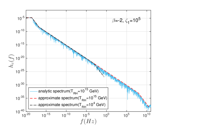
Figure 1: The comparison between the analytic (solid line) and approximate (dashed line) spectra of RGWs with a fixed parameter set of $\beta=-2$, $\zeta_{1}=10^{-5}$ and $T_{\rm{RH}}=10^{15}$ GeV. The approximate spectrum (dot-dashed line) of RGWs with $T_{\rm{RH}}=10^{4}$ GeV was also plotted for comparison.

3.2 Constraints on $\beta$ by pulsar timing arrays and the very early universe

PTA experiments have set constraints on GW background (Bertotti et al. 1983; Kaspi et al. 1994;Thorsett & Dewey 1996; McHugh et al. 1996; Jenet et al. 2006; Hobbs et al. 2009; van Haasteren et al. 2011; Demorest et al. 2013; Zhao et al. 2013). In the data analysis of PTAs, the characteristic strain spectrum of GW background is usually modeled with a power-law form:

$$h_{c}(f)=h_{{\rm yr}}\left(\frac{f}{{\rm yr}^{-1}}\right)^{\alpha},$$ (16)

where $h_{yr}$ is the amplitude at $f={\rm yr}^{-1}$. For the frequency band $10^{-9}\leq f\leq 10^{-6}$ Hz of PTA experiments, the characteristic strain spectrum has the following form (Tong 2012):

$$h_{c}(f)=\frac{A}{\sqrt{2}}\left(\frac{f}{f_{H}}\right)^{1+\beta}\left(\frac{f_{H}}{f_{2}}\right)(1+z_{E})^{-\frac{2+\gamma}{\gamma}}.$$ (17)

With the help of Eq. (15), Eq. (17) can be rewritten as

$$h_{c}(f)=\sqrt{\frac{\Delta_{\mathcal{R}}^{2}(k_{0})r}{2}}\left(\frac{f_{H}^{2}}{f_{0}f_{2}}\right)\left(\frac{f}{f_{0}}\right)^{1+\beta}(1+z_{E})^{-\frac{2+\gamma}{\gamma}}.$$ (18)

Note that $f/f_{0}\gg 1$ in the pulsar timing frequency band. Comparing Eq.(16) and Eq.(18) tells that the power-law index is related to the inflation index via

$$\alpha=1+\beta.$$ (19)

Improving the earlier work (eg. Kaspi et al. 1994), Jenet et al. 2006 developed a frequentist technique of statistics, and have placed an upper limit on $h_{yr}$ for different values of $\alpha$. Recently, Shannon et al. 2013 gave an upper limit $h_{yr}<2.4\times 10^{-15}$ at the $95\%$ confidence level for $\alpha=-2/3$ using data from PPTA and that available observations from the Arecibo observatory. Even though this limit is intended for supermassive black hole binaries, one can equivalently translate it to the case of RGWs, which leads to $h_{yr}<1.0\times 10^{-15}$ for $\alpha=-1$. Note that these limits are independent of $H_{0}$. Fig. 2 gives the upper limit curves of $h_{yr}(\alpha)$ for PPTA at different phases. The PPTA(2006) and the future PPTA obtained from the simulated data of the potential 20 pulsars for the future goal of the PPTA timing are taken from Jenet et al. 2006. To constrain the parameter $\alpha$, $h_{c}(\rm{yr}^{-1})$ with $r=0.2$ was also plotted. As shown in Tong et al. 2014, the condition $h_{c}({\rm yr}^{-1})<h_{yr}(\alpha)$ leads to an upper limit of $\alpha$ (or $\beta$) for a given $r$. Since $r=0.2$ is set in this paper, the PPTA(2013) gives an upper limit $\alpha<-0.70$ ($\beta<-1.70$). Comparably, PPTA(2006) gives an upper limit $\alpha<-0.63$ ($\beta<-1.63$), and the future PPTA will give a limit $\alpha<-0.76$ ($\beta<-1.76$).

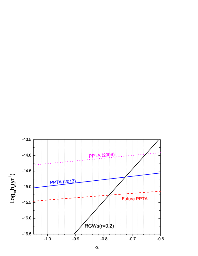
Figure 2: The constraints of $\alpha$ given by the PPTA(2006) (Jenet et al. 2006), the PPTA(2013) (Shannon et al. 2013) and the future PPTA (Jenet et al. 2006), respectively, confronting RGWs with $r=0.2$. These constraints are made at the frequency of one cycle per year.

Besides the constraints from PTAs, some other observations also give constraints on RGWs. For example, $\beta$ can be constrained by ground-based laser interferometer (Tong & Zhang 2009; Chen et al. 2014). However, the ground-based laser interferometers respond to RGWs at the frequency range of $10^{2}-10^{3}$ Hz, and the RGWs with high frequencies depend on theoretical models which are not known well. For instance, if we choose $T_{\rm{RH}}=10^{4}$ GeV, there will be no RGWs with frequencies lager than $0.24$ Hz. In addition, BBN and CMB can give constraints on the GW energy density contrast at the time of nucleosynthesis and CMB decoupling, respectively. The constraint from BBN is given by $\Omega_{GW}^{\rm{BBN}}<1.1\times 10^{-5}(N_{\nu}-3)$ (Maggiore 2000), where the effective number of neutrino species at the time of BBN has an upper bound $N_{\nu}-3<1.4$ (Cyburt et al. 2005). On the other hand, CMB gives $\Omega_{GW}^{\rm{CMB}}<1.3\times 10^{-5}$ (Smith et al. 2006). Note that, the lower frequency limits contributing the energy density contrasts for BBN and CMB are different. For BBN $f_{low}\sim 10^{-10}$ Hz, corresponds to the horizon scale at the time of BBN (Allen & Romano 1999); while for CMB $f_{low}\sim 10^{-15}$, corresponds to the horizon scale at the decoupling of CMB (Zhang et al. 2010). However, the upper limit frequency for the two cases is both $f_{1}$. As pointed out above, $f_{1}$ depends of $\zeta_{s}$, and thus depends of $T_{\rm{RH}}$ in turn. So the constraints on $\beta$ given by BBN or CMB depend on $T_{\rm{RH}}$. As shown in Eq. (9), $f_{1}$ also depends on $\zeta_{1}$, however, we found that the limits of $\beta$ constrained by BBN/CMB are nearly independent on $\zeta_{1}$. It can explained that $\zeta_{1}$ only affects the power spectrum in the frequency band ($f_{s}$, $f_{1}$), which contributes very little to the total energy density contrast. It was also demonstrated clearly in Fig. 1 of Tong et al. 2014. Fig. 3 shows the upper limits of $\beta$ constrained by BBN and CMB with varying $T_{\rm{RH}}$. One can see that BBN and CMB almost give the same constraints for the whole range of $T_{\rm{RH}}$. The most stringent constraint is given by $\beta<-1.83$ with $T_{\rm{RH}}=10^{15}$ GeV, which is more stringent than those given by the present PPTA data. However, one should put it in mind that the constraints of $\beta$ given by PTAs are independent of $T_{\rm{RH}}$.

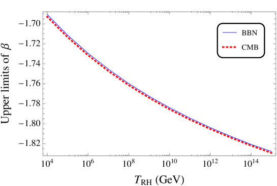
Figure 3: Upper limits of $\beta$ with varying $T_{\rm{RH}}$ given by BBN and CMB , respectively.

4 Imprints of RGWs on pulsar timing

The existence of gravitational waves will change the geodesic of the photons from millisecond pulsars to the observer. Consequently, the TOAs of the electromagnetic signals from pulsars will be perturbed, forming the so-called timing residuals if the effect of RGWs is not taken into account in the timing model. The GW background would lead to a red power-law spectrum of the timing residuals. Even though such red spectra can also be produced by intrinsic noise of pulsars (Verbiest et al. 2009; Shannon & Cordes 2010), inaccuracies in the solar system ephemeris (Champion et al. 2010), or variations in terrestrial time standards (Hobbs et al. 2012), a GW background produces a unique signature in the timing residuals that can be confirmed by observing correlated signals between multiple pulsars widely distributed on the sky (Hellings & Downs 1983; Jenet et al. 2005). However, here we only analyze how RGWs affect the timing residuals of a single pulsar. In principle, if the GW signals are strong enough, one could extract their signals buried in the data of the timing residual measurements after all known effects have been accounted for. On the other hand, even GWs are very weak, one can still constrain the amplitude of GWs with the long-time accumulating data of timing residuals.

The frequency of the signals from a pulsar will be shifted due to the existence of a GW. For a GW propagating in the direction $\hat{\Omega}$, the redshift of the signals from a pulsar in the direction $\hat{p}$ is given by (Detweiler 1979; Anholm et al. 2009)

$$z(t,\hat{\Omega})=\frac{\nu_{e}-\nu_{p}}{\nu_{p}}=\frac{\hat{p}^{i}\hat{p}^{j}}{2(1+\hat{\Omega}\cdot\hat{p})}\Delta h_{ij},$$ (20)

where $\nu_{e}$, $\nu_{p}$ represent the frequencies of the pulse received at the Earth and the pulse emitted at the pulsar, respectively, and

$$\Delta h_{ij}=[h_{ij}(t_{p},\hat{\Omega})-h_{ij}(t_{e},\hat{\Omega})]$$ (21)

is the difference in the metric perturbation traveling along the direction $\hat{\Omega}$ at the pulsar and at the Earth. $t_{p}$ and $t_{e}$ are the times at which the GW passes the pulsar and the Earth, respectively. Note that, the standard Einstein summation convention was used in Eq. (20). The vectors $(t_{e},{\bf{x}}_{e})$ and $(t_{p},{\bf{x}}_{p})$ give the spacetime coordinates of the Solar System barycenter (SSB) and the pulsar, respectively. In the following, we choose a coordinate system that the origin of the space coordinates is located at the SSB, and use $t$ instead of $t_{e}$ denoting the time coordinate. Moreover, the following conventions are often used (Anholm et al. 2009),

$$t_{p}=t-L,\quad{\bf{x}}_{p}=L\hat{p},$$ (22)

where $L$ is the distance of the pulsar away from the SSB. If we assume that the amplitude of the GW is the same at the SSB and the pulsar then $\Delta h_{ij}$ can be written as the following Fourier integration form (Anholm et al. 2009):

$$\Delta h_{ij}(t,\hat{\Omega})=\sum_{A=+,\times}\int_{-\infty}^{\infty}dfe^{i2\pi ft}(e^{-i2\pi fL(1+\hat{\Omega}\cdot\hat{p})}-1)h_{A}(f,\hat{\Omega})\epsilon_{ij}^{A}(\hat{\Omega}),$$ (23)

where $A$ stands for the two polarizations of GWs, and the corresponding tensor $\epsilon_{ij}^{A}(\Omega)$ can be written as

$$\epsilon_{ij}^{+}(\hat{\Omega})=\hat{m}_{i}\hat{m}_{j}-\hat{n}_{i}\hat{n}_{j},\quad\epsilon_{ij}^{\times}(\hat{\Omega})=\hat{m}_{i}\hat{n}_{j}+\hat{n}_{i}\hat{m}_{j},$$ (24)

with $\hat{m},\hat{n}$ unit vectors orthognal to $\hat{\Omega}$ and to each other. One has straightforwardly,

$$\epsilon_{ij}^{A}(\hat{\Omega})\epsilon^{A^{\prime},ij}(\hat{\Omega})=2\delta^{AA^{\prime}}.$$ (25)

If we assume that the stochastic background is isotropic, unpolarized and stationary, the ensemble average of the Fourier amplitudes can be written as

$$\langle\tilde{h}_{A}^{\ast}(f,\hat{\Omega})\tilde{h}_{A^{\prime}}(f^{\prime},\hat{\Omega}^{\prime})\rangle=\frac{1}{16\pi}\delta(f-f^{\prime})\delta^{2}(\hat{\Omega},\hat{\Omega}^{\prime})\delta_{AA^{\prime}}S_{h}(f).$$ (26)

Note that, the spectral density $S_{h}(f)$ defined above is twice as much as that shown in Eq.(8) of Maggiore 2000, and satisfies $S_{h}(f)=S_{h}(-f)$. Here $S_{h}(f)$ is called one-sided spectral density, and it is related to the characteristic strain amplitude as (Maggiore 2000)

$$h_{c}^{2}(f)=fS_{h}(f).$$ (27)

Substitute Eq. (23) into Eq.(20), one has

$$z(t,\hat{\Omega})=\sum_{A}\int_{-\infty}^{\infty}dfe^{i2\pi ft}(e^{-i2\pi fL(1+\hat{\Omega}\cdot\hat{p})}-1)h_{A}(f,\hat{\Omega})F^{A}(\hat{\Omega}),$$ (28)

where

$$F^{A}(\hat{\Omega})\equiv\epsilon_{ij}^{A}(\hat{\Omega})\frac{1}{2}\frac{\hat{p}^{i}\hat{p}^{j}}{1+\hat{\Omega}\cdot\hat{p}}$$ (29)

has been defined. For a stochastic GW background, the total redshift is given by summing over the contributions coming from GWs in every direction (Anholm et al. 2009)

$$z(t)=\int_{S^{2}}d\hat{\Omega}\ z(t,\hat{\Omega}).$$ (30)

The pulsar timing residual is defined as the integral of the redshift

$$R(t)\equiv\int_{0}^{t}dt^{\prime}z(t^{\prime}).$$ (31)

The total relative frequency changes can be divided into two parts:

$$s(t)=z(t)+n(t),$$ (32)

where $z(t)$ is induced by the RGWs and $n(t)$ is the noise intrinsic in the timing measurement which is assumed to be stationary and Gaussian. In addition, we also assume that

$$\langle z(t)\rangle=\langle n(t)\rangle=0,\quad\langle z(t)n(t)\rangle=0,$$ (33)

where the angle brackets denote an expectation value. With the help of Eqs.(26), (28) and (30), the variance of the relative frequency changes is given by

$$\langle z^{2}(t)\rangle\equiv\int_{0}^{\infty}dfS_{z}(f)=F\int_{0}^{\infty}dfS_{h}(f),$$ (34)

where $S_{z}(f)=FS_{h}(f)$ and

$$F\equiv\frac{1}{8\pi}\int_{S^{2}}d\hat{\Omega}\left|e^{i2\pi fL(1+\hat{\Omega}\cdot\hat{p})}-1\right|^{2}\sum_{A}F^{A}(\hat{\Omega})F^{A}(\hat{\Omega}).$$ (35)

Using the definition in Eq.(29), one can easily obtain (Jenet et al. 2011)

$$F=\frac{1}{3}-\frac{1}{8\pi^{2}f^{2}L^{2}}+\frac{\sin{(4\pi fL)}}{32\pi^{3}f^{3}L^{3}}.$$ (36)

The property of $F$ is shown in Fig. 4. It can be seen that $F$ is generally frequency-dependent, however, F will converge to a fixed value $1/3$ when $fL\gtrsim 3$. For pulsar timing experiments, the distances of millisecond pulsars are usually larger than 0.1 kpc, and then $fL>10$ for the frequencies $f>10^{-9}$ Hz. Therefore, one always has $F=1/3$ for pulsar timing experiments. The factor $F$ represents the root-mean-square (rms) signal response averaged over the sky and polarization states.

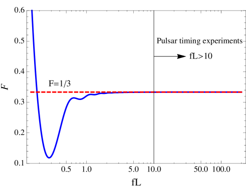
Figure 4: The property of the reduction factor $F$ with different regimes of $fL$. For the pulsar timing experiments, one has $fL>10$.

Similarly, the ensemble average of the Fourier components of the noise satisfies

$$\langle\tilde{n}^{\ast}(f)\tilde{n}(f^{\prime})\rangle=\frac{1}{2}\delta(f-f^{\prime})S_{n}(f),$$ (37)

where the noise spectrum density satisfies $S_{n}(f)=S_{n}(-f)$ with dimension Hz^-1. So, the variance of the noises is

$$\langle n^{2}(t)\rangle=\int_{0}^{\infty}dfS_{n}(f).$$ (38)

Equivalently, the noise level of a GW detector is usually measured by the strain sensitivity $\tilde{h}(f)\equiv\sqrt{S_{n}(f)}$ with dimension Hz^-1/2. For a given signal-to-noise ratio (SNR), one can discuss the ability of a detector to reach the minimum detectable amplitude of RGWs. Under the assumption that the dispersion caused by the interplanetary plasma is adequately calibrated and the intrinsic rotation instability of the pulsar can be negligible or be well understood, the noise spectrum is characterized by the contribution due to the ground clock and a white-timing noise of 100 ns in a Fourier band $+/-0.5$ cycles/day (da Silva Alves & Tinto 2011). The 100 ns level is the current timing goal of PTAs and three pulsars are being timed to this level (Verbiest et al. 2009). Following the noise model discussed in Jenet et al. 2011, the expression for the noise spectrum density of the relative frequency fluctuations is (da Silva Alves & Tinto 2011)

$$S_{zn}(f)=[4.0\times 10^{-31}f^{-1}+3.41\times 10^{-8}f^{2}]\ {\rm{Hz}}^{-1}.$$ (39)

For SNR=1, i.e., $S_{z}(f)/S_{zn}(f)=1$, we plotted the strain sensitivity of the detection on GW background by a single pulsar and the analytic strain amplitude per root Hz (considering the $F$ factor) of RGWs, $h_{c}(f)\sqrt{F/f}$ (Zhang et al. 2010), with different values of $\beta$ in Fig. 5. One can see that it is hard to detect RGWs even for the blue spectrum by an individual pulsar timing method, however, the lower frequencies of RGWs are more hopeful to be detected. Note that, SNR=5 is conventionally taken as detection threshold for PTAs. Thus, the sensitivity curve shown in Fig. 5 should be multiplied a factor of $\sqrt{5}$. Therefore, significant SNR improvements of pulsar timing sensitivities of radio telescopes will be required for reliable detection. There are two ways for this target. First, one can simultaneously timing several pulsars. The SNR can be improved by correlating the data of several pulsars just as the method used in the networks of ground-based interferometers. Second, one should try to suppress the various noises in the timing measurement.

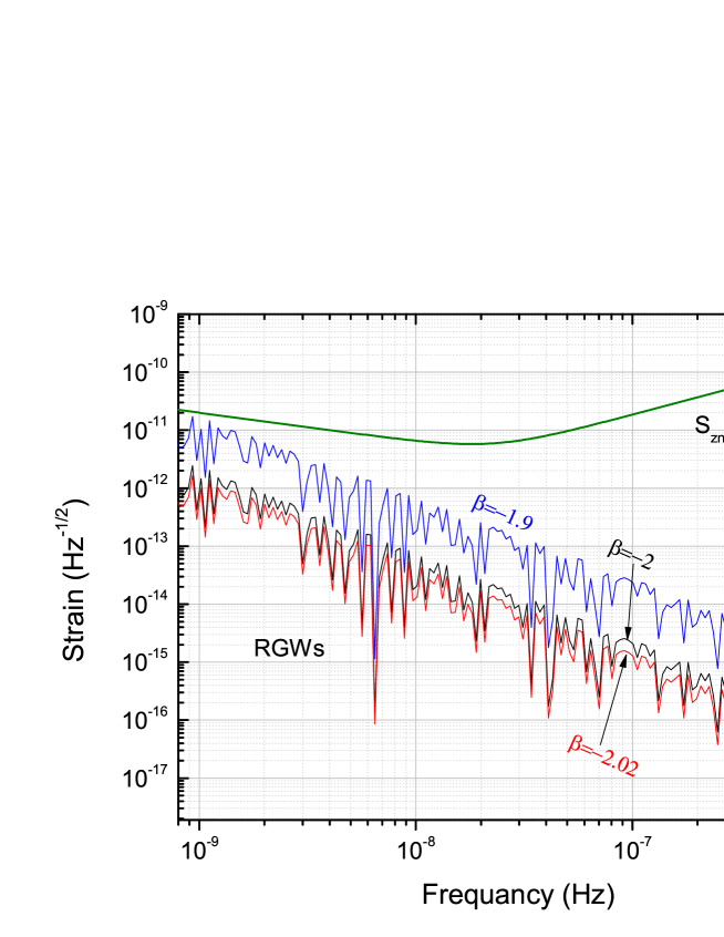
Figure 5: The strain sensitivity curve to be explored by the noise spectrum of the relative frequency fluctuations for a single pulsar timing. The quantities, $h_{c}(f)\sqrt{F/f}$, of RGWs with different parameters $\beta=-1.9$, $\beta=-2.0$ and $\beta=-2.02$, respectively, are also demonstrated for comparison.

The one-sided power spectrum of the induced timing residuals by RGWs, $P(f)$, is defined as (Jenet et al. 2006)

$$\int_{0}^{\infty}P(f)df=\sigma^{2},$$ (40)

where $\sigma^{2}$ is the variance of the timing residuals generated by the stochastic background of RGWs. The power spectrum $P(f)$ is related to the characteristic strain as

$$P(f)=\frac{1}{12\pi}\frac{1}{f^{3}}h_{c}(f)^{2}.$$ (41)

$P(f)$ has the unit of $s^{3}$. Fig. 6 shows the corresponding one-sided power spectrum of the induced timing residuals by RGWs with $\beta=-1.9$, $\beta=-2$ and $\beta=-2.02$, respectively. It can be seen that RGWs with $\beta=-1.9$ leads to a higher $P(f)$ by about two orders of magnitude than that given by RGWs with $\beta=-2$. For $\beta=-1.9$, the power spectrum is as high as $10^{-5}$ $s^{3}$ around $10^{-9}$ Hz. In fact, the integrating limits are determined by observational strategy. The lowest detectable frequency is given by $1/T$, where $T$ is the total time span of the data set. The highest one is determined by the Nyquist sampling rate. If one observes pulsars at an interval of $\Delta t$, then the highest frequency is $2/\Delta t$. For the observation of pulsar timing, $\Delta t$ is typically two weeks, and total data span are assumed to be around 10 years. Then, based on Eq.(40), one has the standard deviation of the timing residuals $\sigma=3.2$ ns, $0.4$ ns and $0.3$ ns for $\beta=-1.9$, $-2$ and $-2.02$, respectively. For comparison, we also calculated the case of $\beta=-1.8$, $\sigma=26.2$ ns, even though $\beta$ is not possibly so large.

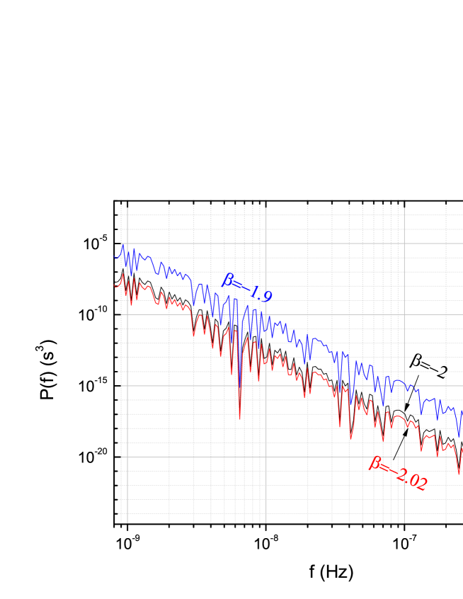
Figure 6: The one-sided power spectra of the induced timing residuals by RGWs with different $\beta$.

5 Summary

In summary, we analyzed the effects of RGWs on the pulsar timing residuals, based on some reasonable parameters constrained by the recent observations of PPTA and the physical processes happened in the very early universe. First of all, we corrected the normalization of RGWs by the CMB observations, and now the spectra are reduced by two orders of magnitude compared to our previous results. Then, we compared the analytic spectrum and the approximate spectrum of RGWs, and we found they matched each other very well. Therefore, one can take advantage of them alternatively. When we constrain the parameter $\beta$ by the PPTA , the approximate spectrum is applied simply; while we calculated the total energy density contrast and the timing residuals induced by RGWs, the analytic spectrum is used. The current PPTA gives a constraint, $\beta<-1.70$, and the future PPTA would give a constraint as $\beta<-1.76$. On the other hand, the constraints of $\beta$ from the BBN/CMB are dependent on some other cosmic parameters, such as the temperature of the reheating process $T_{\rm{RH}}$ and the expansion times of the reheating process $\zeta_{1}$. The strongest constraint from BBN/CMB is $\beta<-1.83$. Note that, the constraints from BBN/CMB are a little bit overestimated because of the effects of the neutrino free-streaming (Weinberg 2004), the $e^{+}e^{-}$ annihilation and the QCD transition (Schwarz 1998; Wang et al. 2008). It is worth to point out that the constraints of $\beta$ from the PPTA are more convincing since it is independent of other parameters. Based on these constraints, we chose $\beta=-1.9$, $\beta=-2$ and $\beta=-2.02$, respectively, for demonstration. We compared the sensitivity curve determined by the ground clock and a white noise of $100$ ns with the predicted RGWs. It was found that RGWs can not be detected by single pulsar timing at present, however, RGWs with frequencies as low as $10^{-9}$ Hz are very hopeful to be detected if the intrinsic red noises were understood. Note that, the noise spectrum discussed in this paper is quite ideal, since many other noise components are not included. We quantitatively calculated the rms residuals induced by RGWs with different values of $\beta$, and found that the rms residuals are $\sigma=3.2$ ns, $0.4$ ns and $0.3$ ns for $\beta=-1.9$, $-2$ and $-2.02$, respectively. Moreover, the rms residual can be as much as $26.2$ ns for $\beta=-1.8$. Besides, we also showed the power spectra of the induced timing residuals by RGWs with different values of $\beta$.

RGWs are a very important and effective tool to exploit the knowledges of the very early universe. All the afore-mentioned constraints on RGWs will help us to know the early universe more clearly. For example, the parameters of expansion times of the reheating process $\zeta_{1}$, the expansion times $\zeta_{s}$ of the radiation-dominated stage and some other parameters would be known better. Even though, the quantum normalization is not employed here in order to give a general result, it should be considered elsewhere for a more complete discussion. Moreover, RGWs act as a key role to connect the subject of cosmology with pulsar timing observations.