Sensor Scheduling in Variance Based Event Triggered Estimation with Packet Drops
Abstract
This paper considers a remote state estimation problem with multiple sensors observing a dynamical process, where sensors transmit local state estimates over an independent and identically distributed (i.i.d.) packet dropping channel to a remote estimator. At every discrete time instant, the remote estimator decides whether each sensor should transmit or not, with each sensor transmission incurring a fixed energy cost. The channel is shared such that collisions will occur if more than one sensor transmits at a time. Performance is quantified via an optimization problem that minimizes a convex combination of the expected estimation error covariance at the remote estimator and expected energy usage across the sensors. For transmission schedules dependent only on the estimation error covariance at the remote estimator, this work establishes structural results on the optimal scheduling which show that 1) for unstable systems, if the error covariance is large then a sensor will always be scheduled to transmit, and 2) there is a threshold-type behaviour in switching from one sensor transmitting to another. Specializing to the single sensor case, these structural results demonstrate that a threshold policy (i.e. transmit if the error covariance exceeds a certain threshold and don’t transmit otherwise) is optimal. We also consider the situation where sensors transmit measurements instead of state estimates, and establish structural results including the optimality of threshold policies for the single sensor, scalar case. These results provide a theoretical justification for the use of such threshold policies in variance based event triggered estimation. Numerical studies confirm the qualitative behaviour predicted by our structural results. An extension of the structural results to Markovian packet drops is also outlined.
I Introduction
The concept of event triggered estimation of dynamical systems, where sensor measurements or state estimates are sent to a remote estimator/controller only when certain events occur, has gained significant recent attention. By transmitting only when necessary, as dictated by performance objectives, e.g., such as when the estimation quality at the remote estimator has deteriorated sufficiently, potential savings in energy usage can be achieved, which are important in networked estimation and control applications.
Related Work: Event triggered estimation has been investigated in e.g. [2, 3, 4, 5, 6, 7, 8, 9, 10, 11, 12, 13], while event triggered control has also been studied in e.g. [14, 15, 16, 17, 18]. Many rules for deciding when a sensor should transmit have been proposed in the literature, such as if the estimation error [3, 5, 7, 10], error in predicted output [6, 13], other functions of the estimation error [4, 11, 12], or the error covariance [9], exceeds a given threshold. These transmission policies often lead to energy savings. However, the motivation for using these rules are usually based on heuristics. Another gap in current literature on event triggered estimation is that mostly the idealized case, where all transmissions (when scheduled) are received at the remote estimator, is considered. Packet drops [19], which are unavoidable when using a wireless communication medium, are neglected in these works, save for some works in event triggered control [16, 18].
In a different line of research, sensor scheduling problems, where one wants to determine a schedule such that at each time instant, one or more sensors are chosen to transmit in order to minimize an expected error covariance performance measure, have been extensively studied, see e.g. [20, 21, 22, 23, 24]. However, these schedules are often constructed ahead of time in an offline manner and do not take into account random packet drops or variations in the state estimates, i.e. are not event triggered. Covariance based switching for scheduling between two sensors was investigated in [25]. Structural results were derived for infinite horizon sensor scheduling problems in [26, 27], which showed that optimal schedules are independent of initial conditions and can be approximated arbitrarily closely with periodic schedules of finite length, with [26] also extending these results to networks with packet drops.
Summary of Contributions: In this paper, we consider a multi-sensor event triggered estimation problem with i.i.d. packet drops, and derive structural properties on the optimal transmission schedule. In particular, the main contributions of this paper are:
-
•
In contrast to previous works on event-triggered estimation, we allow for the more practical situation where sensor transmissions experience random packet drops.
-
•
Rather than specifying the form of the transmission schedule a priori, in this work the transmission decisions are determined by solving an optimization problem that minimizes a convex combination of the expected error covariance and expected energy usage.
-
•
We derive structural results on the form of the subsequent optimal transmission schedule. For transmission schedules which decide whether to transmit local state estimates based only on knowledge of the error covariance at the remote estimator, our analysis shows that 1) for unstable systems, if the error covariance is large, then a sensor will always be scheduled to transmit, and 2) there is a threshold-type behaviour in switching from one sensor transmitting to another.
-
•
Specializing these structural results to the single sensor case shows that a threshold policy, where the sensor transmits if the error covariance exceeds a threshold and does not transmit otherwise, is optimal. This result has also been proved different techniques in our conference contribution [1], and, in a related setup, in [28]. For noiseless measurements and no packet drops, similar structural results were derived using majorization theory for scalar [29] and vector [30] systems respectively.
-
•
In the situation where sensor measurements (rather than local estimates) are transmitted, related structural results are derived, in particular the optimality of threshold policies in the single sensor, scalar case. These structural results provide a theoretical justification for the use of such variance based threshold policies in event triggered estimation. However, for vector systems, we provide counterexamples to show that in general threshold-type policies are not optimal.
-
•
The structural results are extended to Markovian packet drops, where we show that for a single sensor there exist in general two different thresholds, depending on whether packets were dropped or received at the previous time instant.
The remainder of this paper is organized as follows. Section II presents the system model, while the optimization problems are formulated in Section III. Structural results on the optimal transmission scheduling are derived in Sections IV-A and IV-B. The special case of a single sensor is then studied in Section IV-C. The situation where sensor measurements are transmitted is studied in Section V. Numerical studies, including comparisons of our approach with schemes where transmission decisions are made using current sensor measurements, are presented in Section VI. An extension of our structural results to Markovian packet drops is outlined in Section VII.
II System model and Remote Estimation Schemes
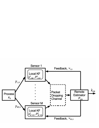
A diagram of the system model is shown in Fig. 1. Consider a discrete time process
| (1) |
where and is i.i.d. Gaussian with zero mean and covariance . There are sensors, with each sensor having measurements
| (2) |
where and is Gaussian with zero mean and covariance .
The noise processes are assumed to be mutually independent.
Each sensor has some computational capability and can run a local Kalman filter. The local state estimates and error covariances
can be computed using the standard Kalman filtering equations at sensors . For the results in Sections II-IV, we will assume that each pair is detectable and the pair is stabilizable. In Section V we will relax this assumption when we consider transmission of sensor measurements, and consequently only detectability of the overall system is required. Let be the steady state value of , and be the steady state value of , as , which both exist due to the detectability assumptions.
Let be decision variables such that if and only if is to be transmitted to the remote estimator at time . Transmitting state estimates when there are packet drops generally gives better estimation performance than transmitting measurements [31, 32], and in the case of a single sensor is the best non-causal strategy [33]. We will focus on the situation where are computed at the remote estimator at time and communicated to the sensors without error via feedback links before transmission at the next time instant ,111This requires synchronization between each sensor and the remote estimator, though not between individual sensors. Note that in wireless communications, online computation of powers at the base station which is then fed back to the mobile transmitters is commonly done in practice [34], at time scales on the order of milli-seconds. see Section II-C on how to take into account losses in the feedback links. Since our interest lies in decision making at the remote estimator, we shall assume that the decisions do not depend on the current value of (or functions of such as measurements and local state estimates). In particular, in this paper we will assume that depends only on the error covariance at the remote estimator, similar to the variance based triggering schemes of [9], see Section III.
At time instances when , sensor transmits its local state estimate over a packet dropping channel. Let be random variables such that if the transmission from sensor at time is successfully received by the remote estimator, and otherwise. It is assumed that the channel is shared such that if more than one sensor transmits at any time, then collisions will occur. Thus, and with probability one if both . We will assume that are i.i.d. Bernoulli with
See Section VII for some results with Markovian packet drops.
II-A Optimal Remote Estimator
At instances where , it is assumed that the remote estimator knows whether the transmission was successful or not, i.e., the remote estimator knows the value . While if , since sensor is not scheduled to transmit at this time, the corresponding is assumed to be of no use to the remote estimator. We can define
as the information set available to the remote estimator at time . Denote the state estimates and error covariances at the remote estimator by:
If a sensor has been scheduled by the remote estimator to transmit at time ,222Since collisions occur if more than one sensor transmits at the same time, we clearly should not schedule more than one sensor to transmit at a time. then the state estimates and error covariances at the remote estimator are updated as follows:
| (3) |
where is the local Kalman filter gain of sensor at time , if , and otherwise. The last three equations in (II-A) compute the quantities:
for where we note that , and .
If no sensors are scheduled to transmit at time , then the state estimates and error covariances are simply updated by:
| (4) |
The derivation of the optimal estimator equations (II-A)-(4) can be found in Appendix -A.
Remark II.1.
In (II-A), the terms and for also need to be computed, since the scheduled sensor will in general change over time.
II-B Suboptimal Remote Estimator
The estimator equations (II-A) are optimal, but difficult to analyze and derive structural results for. A suboptimal estimator that often performs well is a constant gain estimator, which has the form (II-A) but with replaced by the constant gain whenever sensor is scheduled to transmit. Suppose the constant gains are chosen using a similar procedure to [32], where is a fixed point of the following set of equations:
| (5) |
with being the steady state local Kalman gain of sensor . The equations (II-B) are obtained by averaging over in the recursion for (as well as the associated quantities and ) in (II-A), and taking the steady state.
Then we have the following result:
Theorem II.2.
Suppose that is either (i) stable, or (ii) unstable but with , where is an eigenvalue of . Then for each , amongst all possible constant gains satisfying , there is a unique fixed point to the set of equations (II-B) with , and being the unique solution to the equation
Proof.
See Appendix -B ∎
By Theorem II.2, and in particular the fact that for each , the constant gain estimator with gains chosen by solving (II-B) is easily seen to simplify to the following:
| (6) |
where
| (7) |
For the case of two sensors estimating independent Gauss-Markov systems, a similar estimator to (6) was also studied in [23]. We now give some examples comparing the performance of the suboptimal estimator (6) with the optimal estimator (II-A). Consider a two sensor system with parameters
| (8) |
The other parameters are randomly generated: and are matrices with entries drawn from the uniform distribution , and are scalars drawn from , and are drawn from . The sensor that transmits is randomly chosen, with each sensor equally likely to be chosen. Table I gives for the optimal (Opt.) and suboptimal (Subopt.) estimators for different randomly generated sets of parameters, where are obtained by taking the time average over a Monte Carlo simulation of length 100000. We also give values of for the case where measurements are transmitted (Tx. Meas.), which will be studied in Section V. We see that the suboptimal estimator often gives good performance when compared to the optimal estimator.
| Opt. | Subopt. | Tx. Meas. | Opt. | Subopt. | Tx. Meas. |
|---|---|---|---|---|---|
| 3.1410 | 3.2216 | 3.2441 | 2.9906 | 3.0736 | 3.0705 |
| 3.9206 | 4.1434 | 4.2254 | 3.4654 | 3.6203 | 3.5358 |
| 3.6410 | 3.6990 | 3.8116 | 4.3822 | 4.6349 | 4.7211 |
| 3.2056 | 3.3040 | 3.3117 | 3.1704 | 3.2737 | 3.2766 |
| 4.9104 | 5.0146 | 5.1417 | 5.5227 | 5.6810 | 5.7757 |
| 3.5692 | 3.7251 | 3.7227 | 4.5079 | 4.6076 | 4.8558 |
| 4.1598 | 4.2227 | 4.2522 | 3.9006 | 4.0154 | 4.0603 |
| 3.8327 | 3.9082 | 3.9827 | 3.2849 | 3.3567 | 3.3775 |
| 2.9210 | 3.0015 | 2.9704 | 7.0825 | 7.4793 | 7.8819 |
| 3.7504 | 3.9277 | 3.9376 | 3.9697 | 4.1427 | 4.1661 |
II-C Imperfect Feedback Links
We have assumed that the feedback links are perfect, which models the most commonly encountered situation where the remote estimator has more resources than the sensors and can transmit on the feedback links with very low probability of error, e.g., the remote estimator can use more energy or can implement sophisticated channel coding. But interestingly, imperfect feedback links can also be readily incorporated into our framework.
Recall that at each discrete time instant , the remote estimator feeds back the values to notify which sensors should transmit, with at most one in order to avoid collisions. If the feedback command is lost, then the sensor that may have been scheduled to transmit at time will no longer do so, while the other sensors not scheduled to transmit still remain silent. Thus, from an estimation perspective, a dropout in the feedback signal is equivalent to a dropout in the forward link from the sensor to the remote estimator. Assume that the feedback link from the remote estimator to sensor is an i.i.d. packet dropping link with packet reception probability , with the packet drops occurring independently of the forward links from the sensors to the remote estimator. Then for the sensor that is scheduled to transmit, the situation is mathematically equivalent to this sensor transmitting successfully with probability . Thus, the case of imperfect feedback links can be modelled as the case of perfect feedback links with lower packet reception probabilities .
III Optimization of transmission scheduling
In this section we will formulate optimization problems for determining the transmission schedules, that minimize a convex combination of the expected error covariance and expected energy usage, and describe some numerical techniques for solving them. Structural properties of the optimal solutions to these problems will then be derived in Section IV.
Define the countable set
| (9) |
where is the -fold composition of , with the convention that . Then it is clear from (6) that consists of all possible values of at the remote estimator. Note that if the local Kalman filters are operating in steady state, then simplifies to
| (10) |
As foreshadowed in Section II, we will consider transmission policies where depends only on , similar to [9]. From the way in which the error covariances at the remote estimator are updated, see (6), such policies will not depend on , cf. [11]. To take into account energy usage, we will assume a transmission cost of for each scheduled transmission from sensor (i.e., when ).333The transmission cost could represent the energy use in each transmission, but can also be regarded as a tuning parameter to provide some control on how often different sensors will transmit, e.g. increasing will make sensor less likely to transmit. We will consider the following finite horizon (of horizon ) optimization problem:
| (11) |
for some design parameter , where the last line holds since is a deterministic function of and , and is a function of , and . Problem (11) minimizes a convex combination of the trace of the expected error covariance at the remote estimator and the expected sum of transmission energies of the sensors. Due to collisions when more than one sensor is scheduled to transmit, we have
where is defined in (7).
Let the functions be defined recursively as:
| (12) |
Problem (11) can then solved using the dynamic programming algorithm by computing for , providing the optimal . Further call , , and
| (13) |
Then it is clear that the minimization in (III) can be carried out over the set (with cardinality ) instead of the larger set (with cardinality ).
Note that the finite horizon problem (11) can be solved exactly via explicit enumeration, since for a given initial , the number of possible values for , is finite. When the problem has been solved (which only needs to be done once and offline), a “lookup table” will be constructed at the remote estimator which allows for the transmit decisions (for different error covariances) to be easily determined in real time.
We will also consider the infinite horizon problem:
| (14) |
where we now assume that the local Kalman filters are operating in the steady state regime, with . Problem (14) is a Markov decision process (MDP) based stochastic control problem with as the “action” and as the “state” at time .444In (14), “limsup” is used instead of “lim” since in some MDPs the limit may not exist. However, if the conditions of Theorem III.1 are satisfied then the limit will exist. The Bellman equation for problem (14) is
| (15) |
where is the optimal average cost per stage and is the differential cost or relative value function [35, pp.388-389]. For the infinite horizon problem (14), existence of optimal stationary policies can be ensured via the following result:
Theorem III.1.
Suppose that is either (i) stable, or (ii) unstable but with for at least one , where is an eigenvalue of . Then there exist a constant and a function satisfying the Bellman equation (III).
Proof.
See Appendix -C. ∎
Remark III.2.
Remark III.3.
Dynamic programming techniques have also been used to design event triggered estimation schemes in, e.g., [3, 4, 5]. However, these works assume a priori that the transmission policy is of threshold-type, whereas here we don’t make this assumption but instead prove in Section IV that the optimal policy is of threshold-type.
As a consequence of Theorem III.1, Problem (14) can be solved using methods such as the relative value iteration algorithm [35, p.391]. In computations, since the state space is (countably) infinite, one can first truncate in (10) to
| (16) |
which will cover all possible error covariances with up to successive packet drops or non-transmissions. We then use the relative value iteration algorithm to solve the resulting finite state space MDP problem, as follows: For a given , define for the value functions by:
Let be a fixed state (which can be chosen arbitrarily). The relative value iteration algorithm is then given by computing:
| (17) |
for . As , we have , with satisfying the Bellman equation (III). In practice, the algorithm terminates once the differences become smaller than a desired level of accuracy . One then compares the solutions obtained as increases to determine an appropriate value of for truncation of the state space , see Chapter 8 of [36] for further details.
IV Structural properties of optimal transmission scheduling
Numerical solutions to the optimization problems (11) and (14) via dynamic programming or solving MDPs do not provide much insight into the form of the optimal solution. In this section, we will derive some structural results on the optimal solutions to the finite horizon problem (11) and the infinite horizon problem (14) in Sections IV-A and IV-B respectively. To be more specific, we will prove that if the error covariance is large, then a sensor will always be scheduled to transmit (for unstable ), and show threshold-type behaviour in switching from one sensor to another. In Section IV-C, we specialize these results to demonstrate that, in the case of a single sensor, a threshold policy is optimal, and derive simple analytical expressions for the expected energy usage and expected error covariance.
Preliminaries: For symmetric matrices and , we say that if is positive semi-definite, and if is positive definite. In general, only gives a partial ordering on the set defined in (9). Let denote the set of all positive semi-definite matrices. In this section, we will say that a function is increasing if
| (18) |
Note that (18) does not take into account the situations where neither nor holds under the partial order .
Lemma IV.1.
The function is an increasing function of .
Proof.
This is easily seen from the definition. ∎
IV-A Finite Horizon Costs
Lemma IV.2.
The functions defined in (III) are increasing functions of .
Proof.
Theorem IV.3.
(i) The functions defined by
for , , are increasing functions of .
(ii) Define
for , . Suppose that for some , and with , we have
| (20) |
Then for , we have
Proof.
Theorem IV.3 characterizes some structural properties of the optimal transmission schedule over a finite horizon. Theorem IV.3(i) and expression (IV-A) allow one to conclude that for unstable and sufficiently large one will always schedule a sensor to transmit. This is because as increases, so that (21) is always positive for sufficiently large . On the other hand, for stable , we could encounter the situation where sensors are never scheduled to transmit if the costs of transmission are large, since now is always bounded (where the bound could depend on the initial error covariance).
Theorem IV.3(ii) and expression (IV-A) further show that the optimal schedule exhibits threshold-type behaviour in switching from one sensor to another: If for some , sensor is scheduled to transmit, while for some larger , sensor (with ) is scheduled to transmit, then sensor will not transmit . Note however that Theorem IV.3 may not cover all possible situations, since the set given by (9) is in general not a totally ordered set.
For scalar systems (or systems with scalar states and hence scalar ), the set is totally ordered, and Theorem IV.3 and (IV-A) can be used to provide a fairly complete characterization.555The set is also totally ordered in the vector system, single sensor situation in steady state, see Section IV-C. For example, in the situation with two sensors, we have:
Corollary IV.4.
For a scalar system with two sensors, for each , the behaviour of the optimal and falls into exactly one of the following four scenarios:
(i) There exists a such that , for , and for .
(ii) There exists a such that , for , and for .
(iii) There exists some and such that for , for , and for .
(iv) There exists some and such that for , for , and for .
From numerical simulations, one finds that each of the above four scenarios can occur (for different parameter values), see Section VI-B.
IV-B Infinite Horizon Costs
Lemma IV.5.
(i) The functions defined by
for , are increasing functions of .
(ii) Define
for . Suppose that for some , and with , we have and Then for , we have
Proof.
In the infinite horizon situation, any thresholds (which for the finite horizon situation are generally time-varying) become constant, i.e. do not depend on . Thus for example, with the scalar system, two sensor situation considered in Corollary IV.4, one may replace and with and respectively, see also Theorem IV.8.
Remark IV.6.
The structural results derived above allow for significant reductions in the amount of computation required to solve problems (11) and (14). For example, by Theorem IV.3 or IV.5, if for some one has , and for a larger one has , then one can automatically set for all . See also [37] for a related discussion.
When the covariance matrices are not comparable in the positive semi-definite ordering, then the full dynamic programming or value iteration algorithm will need to be run in order to solve the optimization problems. Nevertheless, when the remote estimator (6) is used the computational complexity is not prohibitive. In the case where the local Kalman filters have converged to steady state, which is likely when the horizon is large or if we’re interested in the infinite horizon, the “state space” simplifies to (10), which in numerical approaches is truncated to the set defined in (16). The cardinality of is , which is not exponential in the number of sensors or the horizon . Furthermore, the “action space” defined in (13) has cardinality , which is also linear in .
IV-C Single Sensor Case
In this subsection we will focus on a vector system with a single sensor, and where the local Kalman filter operates in steady state, to further characterize the optimal solutions to problems (11) and (14). For notational simplicity, we will drop the subscript “1” from quantities such as . Recall the set defined by (9), which in the multi-sensor case is not totally ordered in general. For the single sensor case in steady state, becomes:
| (24) |
Lemma IV.7.
In the single sensor case, there is a total ordering on the elements of given by
Proof.
Using (IV-A), Theorems IV.3, IV.5, and Lemma IV.7, we then conclude the following threshold behaviour of the optimal solution:
Theorem IV.8.
(i) In the single sensor case, the optimal solution to the finite horizon problem (11) is of the form:
for some thresholds , where the thresholds may be infinite (meaning that ) when is stable.
(ii) In the single sensor case, the optimal solution to the infinite horizon problem (14) is of the form:
| (25) |
for some constant threshold , where the threshold may be infinite when is stable.
Remark IV.9.
In Theorem IV.8, we could have or equal to , in which case .
Remark IV.10.
As mentioned in the Introduction, Theorem IV.8 was proved in our conference contribution [1] using the theory of submodular functions. Under a related setup that minimizes an expected error covariance measure subject to a constraint on the communication rate, the optimality of threshold policies over an infinite horizon was also proved using different techniques in [28].
Thus in the single sensor case the optimal policy is a threshold policy on the error covariance. This also allows us to derive simple analytical expressions for the expected energy usage and expected error covariance for the single sensor case over an infinite horizon. A similar analysis can be carried out for the finite horizon situation but the expressions will be more complicated due to the thresholds in Theorem IV.8 being time-varying in general.
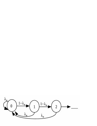
Let be such that , see (25). Note that will depend on the value of chosen in problem (14). Then the evolution of the error covariance at the remote estimator can be modelled as the (infinite) Markov chain shown in Fig. 2, where state of the Markov chain corresponds to the value , with .

The transition probability matrix for the Markov chain can be written as:
For , one can easily verify that this Markov chain is irreducible, aperiodic, and with all states being positive recurrent. Then the stationary distribution
where is the stationary probability of the Markov chain being in state , exists and can be computed using the relation . We find after some calculations that , and , and so
Hence
We can now derive analytical expressions for the expected energy usage and expected error covariance. For the expected energy usage, since the sensor transmits only when the Markov chain is in states , an energy amount of is used in reaching the states corresponding to . Hence
| (26) |
For the expected error covariance, we have
| (27) |
which can be computed numerically. Under the assumption that , will be finite, by a similar argument as that used in the proof of Theorem III.1.
V Transmitting measurements
In this section we will study the situation where sensor measurements instead of local state estimates are transmitted to the remote estimator. In particular, we wish to derive structural results on the optimal transmission schedule. An advantage with transmitting measurements is that detectability at each sensor is not required, but just the detectability of the overall system [9]. In addition, local Kalman filtering at the individual sensors is not required. The optimal remote estimator when sending measurements also has a simpler form than the optimal remote estimator derived in (II-A) when sending state estimates (though not as simple as the suboptimal estimator (6)), which makes it amenable to analysis. Our descriptions of the model and optimization problem below will be kept brief, in order to proceed quickly to the structural results.
V-A System Model
The process and measurements follow the same model as in (1)-(2). Instead of assuming that the individual sensors are detectable, we will now merely assume that is detectable, where is the matrix formed by stacking on top of each other.
Let be decision variables such that if the measurement (rather than the local state estimate) is to be transmitted to the remote estimator at time , and if there is no transmission. As before (see Fig. 1), the transmit decisions are to be decided at the remote estimator and assumed to only depend on the error covariance at the remote estimator.
At the remote estimator, if no sensors are scheduled to transmit, then the state estimates and error covariances are updated by (4). If sensor has been scheduled by the remote estimator to transmit at time then the state estimates and error covariances at the remote estimator are now updated as follows:
| (28) |
where . We can thus write:
| (29) |
where as before, and
| (30) |
for . In (29) the recursions are given in terms of and rather than and , since the resulting expressions are more convenient to work with.
V-B Optimization of Transmission Scheduling
We consider transmission policies that depend only on . The finite horizon optimization problem is:
| (31) |
where we can compute
with defined in (7) and defined in (30). Let the functions be defined as:
| (32) |
Problem (31) can be solved using the dynamic programming algorithm by computing for , with the optimal .
The infinite horizon problem can be formulated in a similar manner but will be omitted for brevity.
V-C Structural Properties of Optimal Transmission Scheduling
Much of this subsection is devoted to proving Theorem V.2, which is the counterpart of Theorem IV.3(i) for scalar systems, and in particular establishes the optimality of threshold policies in the single sensor, scalar case. However, for vector systems we will give a counterexample (Example V.4) to show that, in general, the optimal policy is not a simple threshold policy. The counterpart of Theorem IV.3(ii) also turns out to be false when measurements are transmitted, and we will give another counterexample (Example V.5) to illustrate this.
The following results will assume scalar systems, thus , and are all scalar.
Lemma V.1.
Let be a function formed by composition (in any order) of any of the functions where
and is the identity function. Then:
(i) is either of the affine form
| (33) |
or the linear fractional form
| (34) |
(ii) is an increasing function of , for .
Proof.
(i) We prove this by induction. Firstly, has the form (33), has the form (33), and
has the form (34) since .
Now assume that , which is a composition of the functions , has the form of either (33) or (34). Then we will show that and also has the form of either (33) or (34). For notational convenience, let us write
for some , and
for some with , which can be achieved as shown at the beginning of the proof.
If has the form (34), then
has the form (34), since . Finally,
has the form (34), since .
(ii) By part (i), we know that is either of the form
(33) or (34).
If has the form (33), then
will be an increasing function of , since
can be easily checked to be an increasing function of .
If has the form (34), then it can be verified after some algebra that
since . Hence is an increasing function of . ∎
Theorem V.2.
The functions
for , are increasing functions of .
Proof.
The functions are equivalent to
| (35) |
As stated in the proof of Lemma V.1(ii), can be easily verified to be an increasing function of . Thus Theorem V.2 will be proved if we can show that is an increasing function of for all and .
In fact, we will prove the stronger statement (see Remark V.3) that is an increasing function of for all and , where is a function formed by composition of any of the functions . The proof is by induction. The case of is clear. Now assume that for ,
holds for . We have
| (36) |
In the minimization of (V-C) above, if the optimal (recall the notation of (13)), then
where the last inequality holds by Lemma V.1 (ii), the induction hypothesis, and the fact that is a composition of functions of the form . If instead the optimal , then by a similar argument
| (37) |
Remark V.3.
The reason for proving in Theorem V.2 the stronger statement that is an increasing function of , is that if we carry out the arguments in (V-C) using just , then in (V-C) we end up needing to show statements such as and , neither of which are covered by the weaker induction hypothesis that holds for .
∎
Theorem V.2 is the counterpart of Theorem IV.3(i), for estimation schemes where measurements are transmitted. Referring back to (V-B), is the cost function when no sensors transmit, while is the cost function when sensor transmits. Theorem V.2 thereby establishes that the cost difference between not transmitting and sensor transmitting increases with , and in particular implies the optimality of threshold policies in the single sensor, scalar case. This provides a theoretical justification for the variance based triggering strategy proposed in [9].
For vector systems, it is well known from Kalman filtering that when measurements are transmitted, the error covariance matrices are only partially ordered. One might hope that Theorem V.2 will still hold for vector systems, but in general this is not the case, as the following counterexample shows.
Example V.4.
Consider the case and sensor, so that we are interested in the function (35) with :
Suppose we have a system with parameters
, . Let
Then one can easily verify that , but that
so the function is not an increasing function of .
For vector systems with scalar measurements, a threshold policy was considered in [9], where a sensor would transmit if exceeded a threshold. Since implies , the above example also shows that such a threshold policy is in general not optimal when measurements are transmitted (under our problem formulation of minimizing a convex combination of the expected error covariance and expected energy usage).
Recall the property implied by Theorem IV.3(ii), namely that if for some , sensor is scheduled to transmit, while for some larger , sensor (with ) is scheduled to transmit, then sensor will not transmit . As illustrated below, this property does not hold when measurements are transmitted, even for scalar systems.
Example V.5.
Consider a system with 2 sensors, with parameters , , , , , , . Again look at the case . Then comparing the functions , , and (corresponding respectively to the cases when no sensor transmits, sensor 1 transmits and sensor 2 transmits), we can verify that the optimal strategy is for no sensor to transmit when , sensor 2 to transmit when , sensor 1 to transmit when , but sensor 2 will again transmit when .
V-D Transmitting State Estimates or Measurements
There are advantages and disadvantages to both scenarios of transmitting state estimates or measurements, which we will summarize in this subsection. Sending measurements is more practical when the sensor has limited computation capabilities. Furthermore, detectability at individual sensors is not required. However, as mentioned in Section II, transmitting state estimates outperforms sending of measurements. From Table I, we can see that the optimal estimator when sending estimates outperforms sending of measurements in all cases, while the suboptimal estimator also outperforms the sending of measurements in many cases.
The optimization problems in the infinite horizon situation are also less computationally intensive in the case where state estimates are transmitted and the remote estimator (6) is used. As mentioned in Remark IV.6, the set has a simple form in steady state, which in practice can be easily truncated to a finite set . On the other hand, when measurements are transmitted, the set of all possible values of the error covariance is difficult to determine in the infinite horizon case. Hence it is difficult to discretize the set of all positive semi-definite matrices (which the error covariance matrices will be a subset of) efficiently, and the computational complexity of the associated optimization problems can be very high.
VI Numerical studies
VI-A Single Sensor
We consider an example with parameters
in which case
The packet reception probability is chosen to be , and the transmission energy cost .
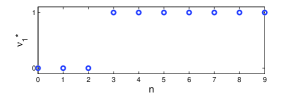
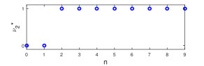
We first consider the finite horizon problem, with and , and with the local Kalman filter operating in steady state. Figs. 3 and 4 plots respectively the optimal and (i.e. and ) for different values of , which we recall represents the different values that the error covariance can take. In agreement with Theorem IV.8, we observe a threshold behaviour in the optimal . In this example we have and ; the thresholds are in general different for different values of .
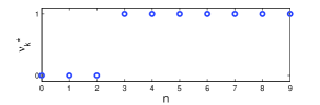
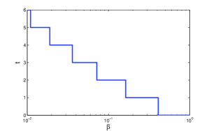
We next consider the infinite horizon problem, with . Fig. 5 plots the optimal for different values of , where we again see a threshold behaviour, with .
In Fig. 6 we plot the values of the thresholds for different values of . As increases, the relative importance of minimizing the error covariance (vs the energy usage) is increased, thus one should transmit more often, leading to decreasing values of the thresholds.
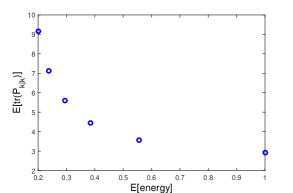
Finally, in Fig. 7 we plot the trace of the expected error covariance vs the expected energy, obtained by solving the infinite horizon problem for different values of , with the values computed using the expressions (26) and (27). Note that the plot is discrete as in (26) and (27), see also Fig. 6.
VI-B Multiple Sensors
We first consider a two sensor, scalar system with parameters , , , , , . We solve the infinite horizon problem with . Fig. 8 plots the optimal and for different values of , with transmission energies . The behaviour corresponds to scenario (i) of Corollary IV.4.
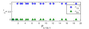
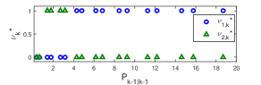
Fig. 9 plots the optimal and for different values of , but with transmission energies . With these parameters, the behaviour corresponds to scenario (iii) of Corollary IV.4. The remaining scenarios (ii) and (iv) of Corollary IV.4 can be illustrated by, e.g., swapping the parameter values of sensors 1 and 2.
VI-C Performance Comparison
Here we will compare the performance of our approach with a scheme similar to that investigated in [5] (see also [10]) that transmits when the difference between the state estimates at sensor and the remote estimator exceeds a threshold .666The scheme is not exactly the same as in [5] since here we also consider random packet drops. In order to avoid collisions, which from simulation experience will greatly deteriorate performance, we allow each sensor to transmit (if it exceeds the threshold ) once every time steps in a round-robin fashion. Specifically,
| (38) |
where is the remote estimate at time .
When the decisions depend on the state estimates, the optimal estimator is generally nonlinear [8, 11]. In the spirit of (6), we consider a suboptimal estimator given by
| (39) |
With this scheme the decision on whether to transmit is made by the sensor (rather than the remote estimator). The sensor has access to its local state estimate, but also requires knowledge of the remote estimate. In the single sensor case, the sensor can reconstruct the remote estimate provided the values of are fed back to the sensor before transmission at time . However, in the multiple sensor case simply feeding back is not enough for the sensors to reconstruct the remote estimate, and it appears that one requires the entire state estimate to be fed back to the sensors in order to implemement this scheme. Thus the scheme (38)-(39) is not intended as a practical scheme for the multi-sensor case, but is only used here for performance comparison with our approach that schedules transmit decisions at the remote estimator.
We consider the two sensor, vector system with parameters
The packet reception probabilities are , , and the transmission energies are . In Fig. 10 we plot the trace of the expected error covariance vs the expected total energy, obtained by solving the infinite horizon problem (14) for different values of . We compare the performance with the scheme (38)-(39) for different values of the thresholds and , with .
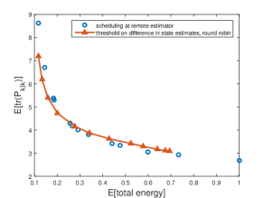
For smaller expected energies, the scheme of (38)-(39) performs better due to the utilization of additional information in the local state estimates, but as stated before requires feedback of the full remote state estimates in order to implement. The approach proposed in Sections II-III performs better when a smaller expected error covariance specification (with corresponding higher expected energy) is required. Furthermore, scheduling at the remote estimator doesn’t require feedback of the remote estimates, but only feedback of the decision variables , which takes values of either 0 or 1 (i.e., one bit of information).
VII Markovian packet drops
So far we have considered i.i.d. packet drops. In this section we briefly outline how our results extend to the case when state estimates are transmitted and the packet loss processes are Markovian. For notational simplicity, we restrict ourselves to the single sensor situation with the local Kalman filter operating in steady state, where the packet loss process is a Markov chain, with transition probabilities and . The probabilities and are also known as, respectively, the failure and recovery rates [39]. We shall consider transmission decisions dependent only on and , in which case the remote estimator equations will still have the form
The finite horizon problem becomes:
| (40) |
for some , where now
The infinite horizon problem is:
| (41) |
The following results can be derived:
Lemma VII.1.
Let the functions be defined recursively for as:
and the functions and as:
Then the functions and are decreasing functions of .
Proof.
Similar to Lemma IV.2, we can show that and are both increasing functions of . One can also easily verify that
and
which can both be shown to be decreasing functions of . ∎
Lemma VII.1 implies that in the finite horizon problem (40), for each there exist two (in general different) thresholds and , , such that when then if and only if ; and when then if and only if .
For the infinite horizon problem (41), arguing in a similar manner as in the proof of Lemma IV.5, the optimal policy will be such that when then if and only if ; and when then if and only if , for some constant thresholds and . Similar to Remark IV.6, knowing that the optimal policy is a threshold policy can lead to significant computational savings when solving problems (40) and (41).
VIII Conclusion
This paper has studied an event based remote estimation problem using multiple sensors, with sensor transmissions over a shared packet dropping channel, where at most one sensor may transmit at a time. By considering an optimization problem for transmission scheduling that minimizes a convex combination of the expected error covariance at the remote estimator and the expected energy across the sensors, we have derived structural properties on the form of the optimal solution, when either local state estimates or sensor measurements are transmitted. In particular, our results show that in the single sensor case a threshold policy is optimal. Possible extensions of this work include the consideration of event triggered estimation with energy harvesting capabilities at the sensors [30, 40], channels where multiple sensors can transmit at the same time, and efficient ways to solve the optimal transmission scheduling problem in the case when measurements are transmitted.
-A Derivation of Optimal Estimator Equations (II-A)
Note first that for the local Kalman filters at the sensors, we have, ,
| (42) |
from which one can obtain
| (43) |
The remote estimator has the form
when sensor is scheduled to transmit. We can write
| (44) |
| (45) |
Let us use the shorthand . Then we have the recursion given in (46).
| (46) |
The recursions for in the optimal estimator equations (II-A) can then be extracted from (46) and (45). It remains to determine the optimal gains . When , we have irrespective of . When , we have
Choosing to minimize the expression for , e.g. by differentiating with respect to (see [41]), we find that if
and
otherwise.
-B Proof of Theorem II.2
We first note that if , then the first equation of (II-B) becomes
which is a Lyapunov equation, that has a unique solution if either (i) is stable, or (ii) is unstable but with
Next, we will show that the second equation of (II-B) also has a solution , irrespective of the value of . We begin by recalling the following expressions for the error covariance and Kalman gain for the local Kalman filter at sensor :
| (47) |
Since we can use (47) to show that
and
we have
Thus the equation
has as a fixed point (irrespective of the value of ). Since for the local Kalman filters , and by assumption , uniqueness of the fixed point can be shown by a similar argument as in p.65 of [42].
It remains to show that . With , we now have from (II-B) that
Similar to above, we can show that
and hence
-C Proof of Theorem III.1
We will verify the conditions (CAV*1) and (CAV*2) given in Corollary 7.5.10 of [36], which guarantee the existence of solutions to the Bellman equation for average cost problems with countably infinite state space. Condition (CAV*1) says that there exists a standard policy777 is a standard policy if there exists a state such that the expected first passage time from to satisfies , and the expected first passage cost from to satisfies . such that the recurrent class of the Markov chain induced by is equal to the whole state space . Condition (CAV*2) says that given , the set is finite, where is the cost at each stage when in state and using action .
We first restrict ourselves to the case of a single sensor . To verify (CAV*1), let be the policy that always transmits, i.e. . Let state of the induced Markov chain correspond to the value , where we define . The state diagram of the induced Markov chain is given in Fig 11, with state space .
Let . Then the expected first passage time from state to state is
The expected cost of a first passage from state to state is
| (48) |
For stable , the infinite series above always converges. To show convergence of the infinite series for unstable , note that the scenario where sensor always transmits to the remote estimator, with packet reception probability , corresponds to the situation studied in [32, 31]. By computing the stationary probabilities of the Markov chain in Fig. 11, we can show that the expected error covariance can be written as . From the stability results of [32, 31], we know that is bounded if and only if . Thus
when .
Hence is a standard policy. Furthermore, one can see from Fig. 11 that the positive recurrent class of the induced Markov chain is equal to , which verifies (CAV*1).
Since the cost per stage corresponds to , condition (CAV*2) can also be easily verified. This thus proves the existence of solutions to the infinite horizon problem in the case of a single sensor .
For the general case with multiple sensors, if at least one sensor satisfies , then solutions to the infinite horizon problem will exist, since restricting to this sensor already guarantees the existence of solutions.
References
- [1] A. S. Leong, S. Dey, and D. E. Quevedo, “On the optimality of threshold policies in event triggered estimation with packet drops,” in Proc. Europ. Contr. Conf., Linz, Austria, Jul. 2015, pp. 921–927.
- [2] Y. Xu and J. P. Hespanha, “Optimal communication logic in networked control systems,” in Proc. IEEE Conf. Decision and Control, Paradise Islands, Bahamas, Dec. 2004, pp. 842–847.
- [3] O. C. Imer and T. Başar, “Optimal estimation with limited measurements,” in Proc. IEEE Conf. Decision and Control, Seville, Spain, Dec. 2005, pp. 1029–1034.
- [4] R. Cogill, S. Lall, and J. P. Hespanha, “A constant factor approximation algorithm for event-based sampling,” in Proc. American Contr. Conf., New York City, Jul. 2007, pp. 305–311.
- [5] L. Li, M. Lemmon, and X. Wang, “Event-triggered state estimation in vector linear processes,” in Proc. American Contr. Conf., Baltimore, MD, Jun. 2010, pp. 2138–2143.
- [6] S. Trimpe and R. D’Andrea, “An experimental demonstration of a distributed and event-based state estimation algorithm,” in Proc. IFAC World Congress, Milon, Italy, Aug. 2011, pp. 8811–8818.
- [7] J. Weimer, J. Araújo, and K. H. Johansson, “Distributed event-triggered estimation in networked systems,” in Proc. IFAC Conf. Analysis and Design of Hybrid Systems, Eindhoven, Netherlands, Jun. 2012, pp. 178–185.
- [8] J. Sijs and M. Lazar, “Event based state estimation with time synchronous updates,” IEEE Trans. Autom. Control, vol. 57, no. 10, pp. 2650–2655, Oct. 2012.
- [9] S. Trimpe and R. D’Andrea, “Event-based state estimation with variance-based triggering,” IEEE Trans. Autom. Control, vol. 59, no. 12, pp. 3266–3281, Dec. 2014.
- [10] M. Xia, V. Gupta, and P. J. Antsaklis, “Networked state estimation over a shared communication medium,” in Proc. American Contr. Conf., Washington, DC, Jun. 2013, pp. 4134–4319.
- [11] J. Wu, Q.-S. Jia, K. H. Johansson, and L. Shi, “Event-based sensor data scheduling: Trade-off between communication rate and estimation quality,” IEEE Trans. Autom. Control, vol. 58, no. 4, pp. 1041–1046, Apr. 2013.
- [12] D. Han, Y. Mo, J. Wu, B. Sinopoli, and L. Shi, “Stochastic event-triggered sensor scheduling for remote state estimation,” in Proc. IEEE Conf. Decision and Control, Florence, Italy, Dec. 2013, pp. 6079–6084.
- [13] S. Trimpe, “Stability analysis of distributed event-based state estimation,” in Proc. IEEE Conf. Decision and Control, Los Angeles, CA, Dec. 2014, pp. 2013–2019.
- [14] K. J. Åström and B. M. Bernhardsson, “Comparison of Riemann and Lebesgue sampling for first order stochastic systems,” in Proc. IEEE Conf. Decision and Control, Las Vegas, NV, Dec. 2002, pp. 2011–2016.
- [15] P. Tabuada, “Event-triggered real-time scheduling of stabilizing control tasks,” IEEE Trans. Autom. Control, vol. 52, no. 9, pp. 1680–1685, Sep. 2007.
- [16] M. Rabi and K. H. Johansson, “Scheduling packets for event-triggered control,” in Proc. Europ. Contr. Conf., Budapest, Hungary, Aug. 2009, pp. 3779–3784.
- [17] C. Ramesh, H. Sandberg, and K. H. Johansson, “Design of state-based schedulers for a network of control loops,” IEEE Trans. Autom. Control, vol. 58, no. 8, pp. 1962–1975, Aug. 2012.
- [18] D. E. Quevedo, V. Gupta, W.-J. Ma, and S. Yüksel, “Stochastic stability of event-triggered anytime control,” IEEE Trans. Autom. Control, vol. 59, no. 12, pp. 3373–3379, Dec. 2014.
- [19] B. Sinopoli, L. Schenato, M. Franceschetti, K. Poolla, M. I. Jordan, and S. S. Sastry, “Kalman filtering with intermittent observations,” IEEE Trans. Autom. Control, vol. 49, no. 9, pp. 1453–1464, September 2004.
- [20] V. Gupta, T. H. Chung, B. Hassibi, and R. M. Murray, “On a stochastic sensor selection algorithm with applications in sensor scheduling and sensor coverage,” Automatica, vol. 42, no. 2, pp. 251–260, 2006.
- [21] L. Shi, P. Cheng, and J. Chen, “Optimal periodic sensor scheduling with limited resources,” IEEE Trans. Autom. Control, vol. 56, no. 9, pp. 2190–2195, Sep. 2011.
- [22] Y. Mo, E. Garone, A. Casavola, and B. Sinopoli, “Stochastic sensor scheduling for energy constrained estimation in multi-hop wireless sensor networks,” IEEE Trans. Autom. Control, vol. 56, no. 10, pp. 2489–2495, Oct. 2011.
- [23] L. Shi and H. Zhang, “Scheduling two Gauss-Markov systems: An optimal solution for remote state estimation under bandwidth constraint,” IEEE Trans. Signal Process., vol. 60, no. 4, pp. 2038–2042, Apr. 2012.
- [24] M. F. Huber, “Optimal pruning for multi-step sensor scheduling,” IEEE Trans. Autom. Control, vol. 57, no. 5, pp. 1338–1343, May 2012.
- [25] H. Sandberg, M. Rabi, M. Skoglund, and K. H. Johansson, “Estimation over heterogeneous sensor networks,” in Proc. IEEE Conf. Decision and Control, Cancun, Mexico, Dec. 2008, pp. 4898–4903.
- [26] Y. Mo, E. Garone, and B. Sinopoli, “On infinite-horizon sensor scheduling,” Systems and Control Letters, vol. 67, pp. 65–70, May 2014.
- [27] L. Zhao, W. Zhang, J. Hu, A. Abate, and C. J. Tomlin, “On the optimal solutions of the infinite-horizon linear sensor scheduling problem,” IEEE Trans. Autom. Control, vol. 59, no. 10, pp. 2825–2830, Oct. 2014.
- [28] Y. Mo, B. Sinopoli, L. Shi, and E. Garone, “Infinite-horizon sensor scheduling for estimation over lossy networks,” in Proc. IEEE Conf. Decision and Control, Maui, HI, Dec. 2012, pp. 3317–3322.
- [29] G. M. Lipsa and N. C. Martins, “Remote state estimation with communication costs for first-order LTI systems,” IEEE Trans. Autom. Control, vol. 56, no. 9, pp. 2013–2025, Sep. 2011.
- [30] A. Nayyar, T. Başar, D. Teneketzis, and V. V. Veeravalli, “Optimal strategies for communication and remote estimation with an energy harvesting sensor,” IEEE Trans. Autom. Control, vol. 58, no. 9, pp. 2246–2260, Sep. 2013.
- [31] Y. Xu and J. P. Hespanha, “Estimation under uncontrolled and controlled communications in networked control systems,” in Proc. IEEE Conf. Decision and Control, Seville, Spain, December 2005, pp. 842–847.
- [32] L. Schenato, “Optimal estimation in networked control systems subject to random delay and packet drop,” IEEE Trans. Autom. Control, vol. 53, no. 5, pp. 1311–1317, Jun. 2008.
- [33] V. Gupta, B. Hassibi, and R. M. Murray, “Optimal LQG control across packet-dropping links,” Systems and Control Letters, vol. 56, pp. 439–446, 2007.
- [34] A. F. Molisch, Wireless Communications, 2nd ed. John Wiley & Sons, 2011.
- [35] D. P. Bertsekas, Dynamic Programming and Optimal Control, Volume I, 2nd ed. Massachusetts: Athena Scientific, 2000.
- [36] L. I. Sennott, Stochastic Dynamic Programming and the Control of Queueing Systems. New York: Wiley-Interscience, 1999.
- [37] M. H. Ngo and V. Krishnamurthy, “Optimality of threshold policies for transmission scheduling in correlated fading channels,” IEEE Trans. Commun., vol. 57, no. 8, pp. 2474–2483, Aug. 2009.
- [38] L. Shi, M. Epstein, and R. M. Murray, “Kalman filtering over a packet-dropping network: A probabilistic perspective,” IEEE Trans. Autom. Control, vol. 55, no. 3, pp. 594–604, Mar. 2010.
- [39] M. Huang and S. Dey, “Stability of Kalman filtering with Markovian packet losses,” Automatica, vol. 43, pp. 598–607, 2007.
- [40] M. Nourian, A. S. Leong, and S. Dey, “Optimal energy allocation for Kalman filtering over packet dropping links with imperfect acknowledgments and energy harvesting constraints,” IEEE Trans. Autom. Control, vol. 59, no. 8, pp. 2128–2143, Aug. 2014.
- [41] D. Simon, Optimal State Estimation: Kalman, , and Nonlinear Approaches. New Jersey: Wiley-Interscience, 2006.
- [42] B. D. O. Anderson and J. B. Moore, Optimal Filtering. New Jersey: Prentice Hall, 1979.