Synchronization of coupled stick-slip oscillators

Zusammenfassung

A rationale is provided for the emergence of synchronization in a system of coupled oscillators in stick-slip motion. The single oscillator has a limit cycle in a region of the state space for each parameter set beyond the supercritical Hopf bifurcation. The two-oscillator system that has similar weakly coupled oscillators exhibits synchronization in a parameter range. The synchronization has an anti-phase nature for an identical pair. However, it tends to be more in-phase for a non-identical pair with a rather weak coupling. A system of three identical oscillators (1, 2, and 3) coupled in a line (with two springs $k_{12}=k_{23}$) exhibits synchronization with two of them (1 and 2 or 2 and 3) being nearly in-phase. These collective behaviors are systematically estimated using the phase reduction method.

Synchronization is ubiquitous in nature as there are numerous natural networks of nonlinear dynamical systems (Pikovsky et al., 2003). Because faults that cause earthquakes or seismogenic processes can be described as nonlinear dynamical systems, synchronization may occur in fault behavior (Scholz, 2010). The standard picture for the occurrence of interplate earthquakes is that a fault segment elastically driven by one plate, under the frictional resistance by another plate, exhibits a stick-slip motion that causes near-periodic spikes. A group of such segments can collectively cause recurring earthquakes with some statistical regularity (e.g., Scholz, 2002; Kawamura et al., 2012). Although many factors about the interaction between fault segments are still unknown, some evidence suggests that they can exhibit synchronization (Rubeis et al., 2010). For example, Chelidze et al. (2005) reported that a stick-slip object in a laboratory setting was entrained by a periodic force. Scholz (2010) statistically determined that the occurrence of earthquakes in some regions was clustered. He reported that synchronous clusters of ruptures of several faults were identified in the south Iceland seismic zone, the central Nevada seismic belt, and the eastern California shear zone. Meanwhile, Mitsui and Hirahara (2004) successfully demonstrated that the numerically modeled coupled stick-slip oscillators exhibited some degree of synchronization. They used a simple spring-slider system composed of several mutually coupled stick-slip oscillators to capture the nature of the earthquake generation cycle along the Nankai trough, which is located in a zone of high seismicity where multiple segments that constitute the fault zone have been reported to rupture almost simultaneously (Ishibashi, 2004a). It is worth noting that they found that a pair of coupled oscillators with slightly different parameter sets synchronized even for weak coupling (Fig. 6 of Mitsui and Hirahara (2004)), although their emphasis was on cases with strong coupling between oscillators.

In spite of these observations, there has been little research that provides a specific description of the conditions for synchronization and how phases behave collectively. In this regard, we focus on the time evolution of the phases to elucidate the synchronization dynamics behind such collective behaviors and how phases are locked in the synchronization.

The occurrences of some earthquakes are nearly periodic (e.g., Matsuzawa et al., 2002; Ishibashi, 2004b; Sykes and Menke, 2006); thus, the generation process can be well modeled as a limit-cycle oscillation. The timing of a limit-cycle oscillation can be described by a single phase variable. If the limit-cycles are somehow connected, they should interact with each other and exhibit some collective behavior as a consequence of the attraction or repulsion between them in terms of the phase. The phase reduction method (Kuramoto, 1984) enables us to quantify the rate at which the progress of an oscillator phase is affected by another oscillator, thereby offering a powerful analytical tool to approximate the limit-cycle dynamics as a closed equation for only a single phase variable.

We shall confine our attention to simple systems of only a few oscillators that remain close to a common limit-cycle orbit, rather than the complicated ones that may produce chaotic motion (e.g., Huang and Turcotte, 1990, 1992; Abe and Kato, 2012), so that we can extract some regularity from the collective behavior of the oscillator system. This setting, of assuming almost homogeneous system of limit cycle oscillators, looks reasonable in the light of observations. In fact, there are some seismic zones that consist of fault segments that have quite similar recurrence periods. The deviation of the earthquake generation periods between different segments along the Nankai trough is a few years, much smaller than the periods themselves, $\sim 1\times 10^{2}\mathrm{year}$ (Ishibashi, 2004a). Likewise, Scholz (2010) points out that synchronization occurs within systems of evenly spaced, subparallel faults with very similar slip rates.

In this study, we quantitatively analyze how a single slider oscillates under the rate- and state-dependent friction against a plate motion using a bifurcation analysis and center-manifold reduction method. Then, we identify when and how coupled sliders driven by a plate synchronize as a collective substance using a phase reduction method.

1 The spring-slider-dashpot system

It is well established that a fault segment that can cause earthquakes is well described by a spring-slider system (e.g., Perfettini and Avouac, 2004) subjected to a rate- and state-dependent friction (Dieterich, 1979; Ruina, 1983; Scholz, 1998); this model exhibits a limit cycle oscillation.

Our research interest, therefore, is in spring-coupled sliders (Fig. 1) that are driven by a common plate through spring and dashpot arrangements set for each slider (e.g., Rice, 1993; Cochard and Madariaga, 1994), against the frictional resistance by another plate. The equations of motion for the $i$-th slider are

$$m_{i}\frac{d^{2}x_{i}}{dt^{2}} = k_{i}\left(V_{p}t-x_{i}-x_{i}^{0}\right)-\frac{G}{2c}\left(\frac{dx_{i}}{dt}-V_{p}\right)-\tau_{i}$$ (1)

$$+\sum_{j}k_{ij}\left(x_{j}-x_{i}-x_{ij}^{0}\right),$$

$$\frac{dx_{i}}{dt} = V_{i},$$ (2)

where $x_{i}$ is the position of the slider, $x_{i}^{0}$ and $x_{ij}^{0}$ are the lengths of springs at rest, $k_{i}$ is the spring constant between the slider and plate, $k_{ij}$ is the spring constant between a pair of sliders, $V_{i}$ is the velocity, $G$ is the rigidity, $c$ is the shear wave velocity, and $V_{p}$ is the constant velocity of the plate. The frictional force $\tau_{i}$ has a rate- and state-dependent form that can be represented as (Ruina, 1983; Dieterich and Kilgore, 1994):

$$\tau_{i} = \sigma_{i}\left(\mu^{*}_{i}+a_{i}\log{\frac{V_{i}}{V^{*}}}+b_{i}\log{\frac{\theta_{i}}{\theta^{*}}}\right),$$ (3)

where $a_{i}$ and $b_{i}$ are frictional parameters, $\sigma_{i}$ is the normal stress, $V^{*}$ and $\theta^{*}$ are the arbitrary reference velocity and state, respectively, and $\mu_{i}^{*}$ is a reference frictional coefficient. The state variable $\theta_{i}$ obeys an aging law represented by (Ruina, 1983; Linker and Dieterich, 1992):

$$\frac{d\theta_{i}}{dt} = 1-\frac{V_{i}\theta_{i}}{L_{i}},$$ (4)

where $L_{i}$ is the characteristic length. Under a quasi-static approximation where the inertia $m_{i}d^{2}x_{i}/dt^{2}$ is sufficiently small (Gu et al., 1984; Perfettini and Avouac, 2004; Perfettini et al., 2005; Kano et al., 2010, 2013), the governing equation for $V_{i}$ can be derived as

$$\frac{dV_{i}}{dt} = \frac{k_{i}(V_{p}-V_{i})-\frac{B_{i}}{\theta_{i}}\left(1-\frac{V_{i}\theta_{i}}{L_{i}}\right)}{\frac{A_{i}}{V_{i}}+g}$$ (5)

$$+\sum_{j}\frac{k_{ij}}{{\frac{A_{i}}{V_{i}}+g}}\left(V_{j}-V_{i}\right),$$

where $A_{i}=\sigma_{i}a_{i}$, $B_{i}=\sigma_{i}b_{i}$, and $g=G/(2c)$. In accordance with the typical applications of the model to the seismogenic process, we assume that the parameters are in the range of

$$g>0,\leavevmode\nobreak\ V_{p}>0,$$ (6)

$$(\forall{i}) A_{i}>0,\leavevmode\nobreak\ L_{i}>0,\leavevmode\nobreak\ k_{i}>0,\leavevmode\nobreak\ B_{i}-L_{i}k_{i}>0,$$ (7)

$$(\forall{i\neq j}) k_{ij}=k_{ji}\geq 0.$$ (8)

We also assume that all of the initial states are placed in the first quadrant:

$$(\forall{i})\leavevmode\nobreak\ V_{i}(0)>0,\leavevmode\nobreak\ \theta_{i}(0)>0.$$ (9)

In Section 2, we investigate the basic properties of a single oscillator. After introducing the phase reduction method in Section 3, we analyze the properties of synchronization, which occurs in a two-oscillator system, in Section 4. We mention some extensions to a three-oscillator system in Section 5.

2 The Dieterich-Ruina oscillator

Here, we investigate the basic properties of a single oscillator using the bifurcation and perturbation analyses.

2.1 Governing equations

Dropping the index $i$ in Eqs. (4) and (5) for simplicity, we obtain the following equations describing a single oscillator:

$$\frac{d\theta}{dt} = 1-\frac{V\theta}{L},$$ (10)

$$\frac{dV}{dt} = \frac{k(V_{p}-V)-\frac{B}{\theta}\left(1-\frac{V\theta}{L}\right)}{\frac{A}{V}+g}.$$ (11)

This is a two-dimensional dynamical system with six parameters $(k,V_{p},g,A,B,L)$. Hereafter, the dynamical system described by Eqs. (10) and (11) is called the Dieterich-Ruina oscillator, and the state vector is denoted as $\vec{X}=(\theta,V)^{T}$. For the simplicity of analytical expressions, we use a new parameter set $(\mu,V_{p},C,d,q,L)$ that is defined as

$$C = (A+gV_{p})^{-1},\leavevmode\nobreak\ d=CgV_{p},\leavevmode\nobreak\ q=\sqrt{CLk},$$ (12)

$$\mu = B-A-gV_{p}-Lk,$$ (13)

where $\mu$ serves as a bifurcation parameter. Here, we investigate how the system behaves as $\mu$ changes. This system has a unique equilibrium point at $\vec{X}_{0}=(L/V_{p},V_{p})^{T}$, which is given by the intersection of the nullclines:

$$\mbox{I}:\quad V = \frac{L}{\theta}\quad\mbox{for}\leavevmode\nobreak\ \frac{d\theta}{dt}=0,$$ (14)

$$\mbox{II}:\quad V = \left(\frac{B}{L}-k\right)^{-1}\left(\frac{B}{\theta}-kV_{p}\right)\quad\mbox{for}\leavevmode\nobreak\ \frac{dV}{dt}=0.$$ (15)

One of the important facts concerning the linear structure of the system around an equilibrium point is that the Jacobi matrix $\mathbf{J}$ has a characteristic sign pattern given by

$$\mathbf{J}=\left[\begin{array}[]{cc}-\frac{V_{p}}{L}&-\frac{1}{V_{p}}\\ \frac{V_{p}^{3}(q^{2}+1)}{L^{2}}&\frac{V_{p}}{L}\end{array}\right]+\mu\left[\begin{array}[]{cc}0&0\\ \frac{CV_{p}^{3}}{L^{2}}&\frac{CV_{p}}{L}\end{array}\right]=\left[\begin{array}[]{cc}-&-\\ +&+\end{array}\right],$$ (16)

which represents a substrate-depletion system (Arcuri and Murray, 1986). The two eigenvalues of the Jacobi matrix at $\vec{X}_{0}$ are

$$\lambda_{1,2}=\frac{CV_{p}}{L}\mu\pm\frac{V_{p}}{2L}\sqrt{-4q^{2}+C^{2}\mu^{2}}.$$ (17)

2.2 Stable spiral: $\mu<0$

The equilibrium point is a stable spiral when $-2q/C<\mu<0$ because the eigenvalues of $\mathbf{J}$ are a complex conjugate pair,

$$\lambda_{1,2}=\frac{CV_{p}}{L}\mu\pm\mathrm{i}\frac{V_{p}}{2L}\sqrt{4q^{2}-C^{2}\mu^{2}},$$ (18)

and have a common negative real part.

2.3 Hopf bifurcation: $\mu=0$

At the very instance when $\mu=0$, the equilibrium point begins to lose its stability. The system encounters a Hopf bifurcation because the Jacobi matrix has a pair of imaginary eigenvalues

$$\lambda_{1,2}=\pm\mathrm{i}\frac{V_{p}q}{L}.$$ (19)

The corresponding eigenvectors are

$$\vec{U}=\left[\begin{array}[]{c}\frac{L(\mathrm{i}q-1)}{V_{p}(q^{2}+1)}\\ V_{p}\end{array}\right],$$ (22)

and its complex conjugate, $\overline{\vec{U}}$. $\vec{U}$ and $\overline{\vec{U}}$ span the plane containing linear solutions. By introducing a complex amplitude, $W(t)$, the neutral solution of the system is expressed as

$$\vec{X}(t) = \vec{X}_{0}+\left\{\vec{U}W(t)\exp{\left[\mathrm{i}\omega_{0}t\right]}+\mathrm{c.c.}\right\},$$ (23)

$$\omega_{0} = \frac{V_{p}q}{L},$$ (24)

where $\mathrm{c.c.}$ represents the complex conjugate. The graph containing the solution indicates an elliptic orbital motion, while the complex amplitude is an arbitrary complex constant at this stage ($\mu=0$) if we neglect nonlinear terms.

2.4 Weakly nonlinear: $\mu\gtrsim 0$

When the bifurcation parameter $\mu$ becomes slightly larger than $0$, the equilibrium point becomes an unstable spiral because the eigenvalues of $\mathbf{J}$ are a complex conjugate pair with a common positive real part. Here, we develop an analytical expression for the asymptotic solutions in a weakly nonlinear regime, by expanding Eqs. (10) and (11) as a Taylor series in terms of the deviation $\vec{u}\equiv\vec{X}-\vec{X}_{0}$ (See appendix A), and using $\vec{U}$ in Eq. (22) and its dual, $\vec{U}^{*}$ (a left eigenvector), which is given by:

$$\vec{U}^{*} = \left(-\mathrm{i}\frac{V_{p}(q^{2}+1)}{2Lq},\leavevmode\nobreak\ V_{p}^{-1}\left(\frac{1}{2}-\mathrm{i}\frac{1}{2q}\right)\right).$$ (25)

With the expansion and eigenvectors, we can compute the coefficients for a small-amplitude equation near the Hopf bifurcation following the center-manifold reduction method described in Kuramoto (1984). Assuming the solutions are in the form of Eq. (23), the time evolution of the complex amplitude can be described by the Stuart-Landau equation as

$$\frac{dW}{dt} = \mu\alpha W-\beta\left|W\right|^{2}W,$$ (26)

$$\alpha = \vec{U}^{*}\mathbf{L}_{1}\vec{U}=\frac{CV_{p}}{2L},$$ (27)

$$\beta = -3\vec{U}^{*}\mathbf{N}\left(\vec{U},\vec{U},\overline{\vec{U}}\right)$$ (28)

$$+4\vec{U}^{*}\mathbf{M}\left(\vec{U},\mathbf{M}(\vec{U},\mathbf{L}_{0}^{-1}\mathbf{M}(\vec{U},\overline{\vec{U}})\right)$$

$$+2\vec{U}^{*}\mathbf{M}\left(\overline{\vec{U}},\left(\mathbf{L}_{0}-2\mathrm{i}\omega_{0}\mathbf{I}\right)^{-1}\mathbf{M}(\vec{U},\vec{U})\right)$$

$$= \frac{V_{p}}{2L}\left(d(1-d)+\mathrm{i}\frac{q^{2}(1+2d)(1-d)+d^{2}}{3q}\right).$$

This system encounters a supercritical bifurcation to a stable limit cycle, because the supercriticality condition $\mathrm{Re}\,\beta>0$ is derived from $0<d=gV_{p}/(A+gV_{p})<1$. Note that the type of the bifurcation may have some dependence on the laws of friction and assumptions made on the equation of motion (Gu et al., 1984; Putelat et al., 2010). In the original vector form, the limit-cycle solution of Eq. (26) is given by

$$\vec{X} = \vec{X}_{0}+\left\{\vec{U}R_{s}\exp{\left[\mathrm{i}(\omega_{0}+\tilde{\omega})t\right]}+\mathrm{c.c.}\right\},$$ (29)

$$R_{s} = \sqrt{\frac{\mu\mathrm{Re}\,\alpha}{\mathrm{Re}\,\beta}}=\sqrt{\frac{\mu C}{d(1-d)}},$$ (30)

$$\tilde{\omega} = \mu\mathrm{Re}\,\alpha\left(\frac{\mathrm{Im}\,\alpha}{\mathrm{Re}\,\alpha}-\frac{\mathrm{Im}\,\beta}{\mathrm{Re}\,\beta}\right)$$ (31)

$$= -\mu\frac{CV_{p}}{L}\frac{q^{2}(1+2d)(1-d)+d^{2}}{6qd(1-d)},$$

which graphically describes an elliptic orbital motion. The modulus, $R_{s}$, and frequency shift, $\tilde{\omega}$, are scaled with $\mu^{1/2}$ and $\mu$, respectively.

We performed numerical integrations of Eqs. (10) and (11) to simulate the limit-cycle oscillation near the Hopf bifurcation point for three cases with $\mu=10^{-5}$, $10^{-4}$, and $10^{-3}\mathrm{Nm^{-2}}$. The time integrations were performed with the fourth-order Runge-Kutta scheme containing variable time step-sizes (Press et al., 1992). The rest of the parameters were set according to a previous study by Kano et al. (2010) for an inter-plate earthquake occurred on September 25, 2003 in Hokkaido, Japan: $(V_{p},g,A,B,L)=(3.17\times 10^{-9}\,\mathrm{ms^{-1}},\leavevmode\nobreak\ 5.00\times 10^{6}\,\mathrm{Nm^{-3}s},\leavevmode\nobreak\ 1.50\times 10^{5}\,\mathrm{Nm^{-2}},\leavevmode\nobreak\ 2.20\times 10^{5}\,\mathrm{Nm^{-2}},\leavevmode\nobreak\ 1.00\times 10^{-2}\,\mathrm{m})$; these values also serve as the standard set of parameter values for this study. In Fig. 2, we show the results with the orbits of the limit cycle compared to those derived using Eq. (29). The corresponding orbits are in good agreement when $\mu$ is small.

In the context of seismogenic processes, the analytical solution (Eq. (29)) in the weakly nonlinear regime may offer a simplified description of slow earthquakes (e.g., Yoshida and Kato, 2003; Helmstetter and Shaw, 2009), which can be viewed as sustaining aseismic oscillations in which the slip instability is sufficiently weak (Kawamura et al., 2012). In particular, the frequencies in Eqs. (24) and (31) can be used to evaluate the recurrence intervals of such earthquakes.

2.5 Limit cycle: $\mu>0$

When we increase $\mu$, the system will enter a strongly nonlinear regime. The equilibrium point becomes either an unstable spiral (when $0<\mu<2q/C$) or unstable node (when $\mu>2q/C$). Then, the Poincaré-Bendixson theorem (e.g., Strogatz, 2001) ensures the existence of a limit cycle within some region surrounding the equilibrium point, because we now have an unstable equilibrium point with a surrounding trapping region, $R$. Appendix B describes how flows are trapped into the region. Figure 3 shows an example of a limit cycle orbit derived by numerically integrating Eqs. (10) and (11). The orbit appears more polygonal than elliptical and extends over a wide range in the first quadrant.

3 The phase reduction method

Here, we introduce the phase reduction method for general limit-cycle oscillators, as well as its specific representation for weakly nonlinear oscillators.

3.1 Limit-cycle oscillators

A system of coupled self-sustained oscillators can be described by

$$\frac{d\vec{X}_{i}}{dt} = \vec{F}(\vec{X}_{i})+\delta\vec{f}_{i}(\vec{X}_{i})+\sum_{j\neq i}\vec{g}_{ij}(\vec{X}_{i},\vec{X}_{j}),$$ (32)

where we assume that the system $d\vec{X}/dt=\vec{F}(\vec{X})$ behaves by itself as a limit-cycle oscillator and that the system described by Eq. (32) has an oscillatory behavior similar to it, including the frequency and orbit. Provided that the oscillators have similar properties and are weakly coupled, the phase reduction method (Kuramoto, 1984), shown below, is applicable to the system. Using the period, $T$, and the frequency, $\omega$, for the limit cycle of the system $d\vec{X}/dt=\vec{F}(\vec{X})$, we can define the phase, $\phi$, of a state that is determined up to an integral multiple of $T$, which varies from $0$ to $2\pi$. The time evolution of the phase obeys

$$\frac{d\phi_{i}}{dt} = \omega+\delta\omega_{i}+\sum_{j\neq i}\Gamma_{ij}(\phi_{i}-\phi_{j}),$$ (33)

where $\phi_{i}$ is the phase of the oscillator $i$, $\delta\omega_{i}$ is the frequency deviation of oscillator $i$ from the original limit cycle frequency, and $\Gamma_{ij}$ is the phase coupling function (hereafter, the PCF) between the oscillators $i$ and $j$, which is periodic with a period of $2\pi$. These terms are defined as the averaged values of the deviation terms in Eq. (32) over a period of the limit cycle under the action of phase sensitivity, $\vec{Z}(\phi)$, (a row vector):

$$\delta\omega_{i} = \frac{1}{2\pi}\int_{0}^{2\pi}\vec{Z}(\phi)\delta\vec{f}_{i}(\phi)\,d\phi,$$ (34)

$$\Gamma_{ij}(\psi) = \frac{1}{2\pi}\int_{0}^{2\pi}\vec{Z}(\phi)\vec{g}_{ij}(\phi,\phi-\psi)\,d\phi.$$ (35)

Here, $\vec{Z}(\phi)$ coincides with a left Floquet eigenvector, with eigenvalue 0, for the linearized equation around the limit cycle. Refer to Kuramoto (1984) for the details of the phase reduction method discussed here.

This procedure is applicable to the system containing Dieterich-Ruina oscillators (Eqs. (4) and (5)), provided that both the parameter differences and coupling intensities of the oscillators are small enough to be treated as a perturbation. Substituting the specific functions in Eq. (5) into Eq. (35), we obtain the phase description of the system:

$$\frac{d\phi_{i}}{dt} = \omega+\delta\omega_{i}+\sum_{j\neq i}k_{ij}\hat{\Gamma}\left(\phi_{i}-\phi_{j}\right),$$ (36)

$$\Gamma\left(\psi\right) = k_{ij}\hat{\Gamma}\left(\psi\right)$$ (37)

$$= \frac{k_{ij}}{2\pi}\int_{0}^{2\pi}\frac{V^{*}(\phi)}{A/V(\phi)+g}\left[V(\phi-\psi)-V(\phi)\right]\,d\phi,$$

where $V^{*}$ is the phase sensitivity for $V$. Note that $V$ and $V^{*}$ are defined along a stable orbit of a single oscillator without coupling, which has a frequency $\omega$.

3.2 Weakly nonlinear oscillators

Suppose we have a system of weakly nonlinear oscillators that are identical and mutually coupled. Near the Hopf bifurcation point, each oscillator can be described by Eq. (26) and a coupling term, which is supposed to be small:

$$\frac{dW_{i}}{dt} = \mu\alpha W_{i}-\beta|W_{i}|^{2}W_{i}+\sum_{j\neq i}k_{ij}\gamma(W_{j}-W_{i}).$$ (38)

Normalizing the equations to $t^{\prime}=\left(\mu\mathrm{Re}\,\alpha\right)t$ and $W^{\prime}=\left(\mu\mathrm{Re}\,\alpha/\mathrm{Re}\,\beta\right)^{-\frac{1}{2}}W$, we get

$$\frac{dW^{\prime}_{i}}{dt^{\prime}} = (1+\mathrm{i}c_{0})W^{\prime}_{i}-\left(1+\mathrm{i}c_{2}\right)|W^{\prime}_{i}|^{2}W^{\prime}_{i}$$ (40)

$$+\sum_{j\neq i}k^{\prime}_{ij}(1+\mathrm{i}c_{1})(W^{\prime}_{j}-W^{\prime}_{i}),$$

$$c_{0}=\frac{\mathrm{Im}\,\alpha}{\mathrm{Re}\,\alpha},\quad c_{1}=\frac{\mathrm{Im}\,\gamma}{\mathrm{Re}\,\gamma},$$

$$c_{2}=\frac{\mathrm{Im}\,\beta}{\mathrm{Re}\,\beta},\quad k^{\prime}_{ij}=\frac{k_{ij}\mathrm{Re}\,\gamma}{\mu\mathrm{Re}\,\alpha}.$$

By treating each oscillator as a two-dimensional system with independent variables $\left(\mathrm{Re}\,W^{\prime}_{i},\mathrm{Im}\,W^{\prime}_{i}\right)^{T}$, we can analytically derive the PCF for this complex Ginzburg-Landau-type equation (Kuramoto, 1984):

$$\Gamma_{ij}(\psi) = -k^{\prime}_{ij}\left[(1+c_{1}c_{2})\sin{\psi}+(c_{2}-c_{1})(\cos{\psi}-1)\right].$$ (41)

For the case of the weakly nonlinear Dieterich-Ruina oscillators, (Eqs. (4) and (5) near the Hopf bifurcation point), the coupling coefficient, $\gamma$, is defined in the same manner as $\alpha$ in Eq. (27):

$$\gamma = \vec{U}^{*}\left[\begin{array}[]{cc}0&0\\ 0&\frac{1}{A/V_{p}+g}\end{array}\right]\vec{U}=\left(\frac{1}{2}-\mathrm{i}\frac{1}{2q}\right)\left(\frac{1}{A/V_{p}+g}\right).$$ (44)

Substituting Eqs. (27), (28), and (44) into Eq. (40), we get the coefficients in Eq. (40):

$$c_{0}=0,\quad c_{1}=-\frac{1}{q},\quad c_{2}=\frac{q^{2}(1+2d)(1-d)+d^{2}}{3qd(1-d)},$$

$$k^{\prime}_{ij}=\frac{k_{ij}L}{\mu}\geq 0.$$ (45)

Thus, the PCF (Eq. (41)) for the weakly nonlinear Dieterich-Ruina oscillator is characterized by

$$1+c_{1}c_{2} = -\frac{q^{2}(1-d)^{2}+d^{2}}{3q^{2}d(1-d)}<0,$$ (46)

$$c_{2}-c_{1} = \frac{q^{2}(1+2d)(1-d)+d(3-2d)}{3qd(1-d)}>0.$$ (47)

In particular, the inequality (46) indicates that the coupling has an anti-phase nature ($d\Gamma/d\psi(0)>0,\leavevmode\nobreak\ d\Gamma/d\psi(\pi)<0)$). Figure 4 shows the PCF as a function of the phase with the same parameters as in Fig. 2.

4 Two-oscillator system

Here, we explore when and how synchronization occurs in the system of two mutually coupled Dieterich-Ruina oscillators. We assume the two oscillators are identical except for a slight difference in the value of $B_{i}$. To confirm the applicability of the phase reduction method to the stick-slip oscillator system, we examine the properties of the synchronization in two different ways. First, we observe the synchronization through numerical integrations of a coupled oscillator system. Second, we derive the PCF for the phase equations using the results from the numerical integration of a single oscillator system and its adjoint. Then, we determine some quantities from the plot.

4.1 Numerical Integrations

We performed numerical integrations of a discrete-time version of Eqs. (4) and (5), for a pair of coupled oscillators: a reference oscillator (oscillator 1) and a second oscillator (oscillator 2). Oscillator 1 had the following parameters: $(k,V_{p},g,A,B,L)=(1.00\times 10^{5}\,\mathrm{Nm^{-3}},\leavevmode\nobreak\ 3.17\times 10^{-9}\,\mathrm{ms^{-1}},\leavevmode\nobreak\ 5.00\times 10^{6}\,\mathrm{Nm^{-3}s},\leavevmode\nobreak\ 1.50\times 10^{5}\,\mathrm{Nm^{-2}},\leavevmode\nobreak\ 2.20\times 10^{5}\,\mathrm{Nm^{-2}},\leavevmode\nobreak\ 1.00\times 10^{-2}\,\mathrm{m})$, and the natural frequency was $1.0687876\times 10^{-9}\mathrm{s^{-1}}$. Two identical oscillators are coupled for case 0. For cases 1, 2, and 3, we used oscillator 2 that has the same set of parameters as oscillator 1 except for $B=2.2025\times 10^{5}$, $2.225\times 10^{5}$, and $2.25\times 10^{5}\mathrm{Nm^{-2}}$, respectively. The natural frequencies of oscillator 2 in cases 1, 2, and 3 were $1.0652082\times 10^{-9}\mathrm{s^{-1}}$, $1.0340304\times 10^{-9}\mathrm{s^{-1}}$, and $1.00143857\times 10^{-9}\mathrm{s^{-1}}$, respectively. We used a common coupling strength of $K=k_{12}=k_{21}=3\times 10^{3}\,\mathrm{Nm^{-3}}$ for all cases, based on the one used in Kano et al. (2010), which was derived through the inversion of strain rate from the GPS observation. We also checked that the values of $B$ and $K$ were within the range of application of the phase reduction method (See appendix C). The time integrations are performed using the same method described in Section 2.4. Figure 5 shows the results of case 0, in which the oscillators synchronize at the phase difference $\psi=-3.14$ (anti-phase). Figure 6 shows the results of case 1, in which the oscillators synchronize at the phase difference $\psi=-1.18$ (out-of-phase). Figure 7 shows the results of case 2, in which the oscillators synchronize at the phase difference $\psi=-7.07\times 10^{-3}$ (almost in-phase). Figure 8 shows the results of case 3, in which they exhibit no synchronization. These phase differences and synchronized oscillator frequencies are listed in Table 1.

4.2 Application of the PCF

In this setting, the evolution of the phases can be described as

$$\frac{d\phi_{1}}{dt} = \omega+\delta\omega_{1}+K\hat{\Gamma}\left(\phi_{1}-\phi_{2}\right),$$ (48)

$$\frac{d\phi_{2}}{dt} = \omega+\delta\omega_{2}+K\hat{\Gamma}\left(\phi_{2}-\phi_{1}\right),$$ (49)

where the PCF is defined in Eq. (37), and the difference between the natural frequencies is estimated to be

$$\Delta\omega \equiv \delta\omega_{1}-\delta\omega_{2}$$ (50)

$$= \frac{B_{1}-B_{2}}{2\pi}\int_{0}^{2\pi}\frac{-V^{*}(\phi)/\theta(\phi)}{A/V(\phi)+g}\left(1-\frac{V(\phi)\theta(\phi)}{L}\right)\,d\phi.$$ (51)

Taking the difference between Eqs. (48) and (49), we obtain the time evolution of the phase difference, $\psi=\phi_{1}-\phi_{2}$:

$$\frac{d\psi}{dt} = 2K\left[\frac{\Delta\omega}{2K}+\hat{\Gamma}_{a}(\psi)\right],$$ (52)

$$\hat{\Gamma}_{a}(\psi) \equiv \frac{1}{2}\left(\hat{\Gamma}(\psi)-\hat{\Gamma}(-\psi)\right).$$ (53)

Using a primitive function on the right-hand side of Eq. (52), we find that the phase difference obeys a gradient dynamical system

$$\frac{d\psi}{dt} = -\frac{dU}{d\psi},$$ (54)

$$U(\psi) \equiv -\int_{-\pi}^{\psi}\left[\Delta\omega+2K\hat{\Gamma}_{a}(\zeta)\right]\,d\zeta.$$ (55)

As $t\to\infty$, the state approaches a stable point at the bottom of the potential $U$. The realization of synchronization is equivalent to the existence of a phase difference $\psi_{\mathrm{sync}}$ that satisfies

$$\frac{dU}{d\psi} = -\Delta\omega-2K\hat{\Gamma}_{a}(\psi_{\mathrm{sync}})=0,$$ (56)

subject to

$$\frac{d^{2}U}{d\psi^{2}} = -2K\hat{\Gamma}_{a}^{\prime}(\psi_{\mathrm{sync}})>0.$$ (57)

Taking the average of Eqs. (48) and (49), we obtain the time evolution of the phase average, $\varphi=(\psi_{1}+\psi_{2})/2$:

$$\frac{d\varphi}{dt} = \overline{\omega}\left[1+\frac{K}{\overline{\omega}}\hat{\Gamma}_{s}(\psi)\right],$$ (58)

$$\hat{\Gamma}_{s}(\psi) \equiv \frac{1}{2}\left(\hat{\Gamma}(\psi)+\hat{\Gamma}(-\psi)\right),$$ (59)

where $\overline{\omega}=\omega+\left(\delta\omega_{1}+\delta\omega_{2}\right)/2$. When synchronization is achieved, the frequency is shifted to

$$\left.\frac{d\varphi}{dt}\right|_{\mathrm{sync}} = \overline{\omega}\left[1+\frac{K}{\overline{\omega}}\hat{\Gamma}_{s}(\psi_{\mathrm{sync}})\right].$$ (60)

We calculated the phase sensitivity, $V^{*}$, with a relaxation method (Ermentrout, 1996; Ermentrout and Terman, 2010), using a numerical integration of the adjoint model of the Dieterich-Ruina oscillator. The integration is also performed using a fourth-order Runge-Kutta scheme with variable time-step sizes (Press et al., 1992). Figure 9 shows the phase sensitivity, or the values of $V^{*}$, during a time interval. The value of the sensitivity remains positive for most of the period except at the moment when a slip event occurs. After the slip event, the sensitivity starts to increase for a while, following which it gradually decreases. Using the calculated values of $V$, $\theta$, and $V^{*}$ as functions of phase, we have also calculated the PCF for the oscillator according to Eq. (37). Figure 10(a) shows the PCF as a function of phase. Figure 10(b) shows the PCF on negative and positive half-planes of phase in a logarithmic scale. The PCF is classified as an anti-phase type as in Fig. 4, although the shape does not resemble a sine curve.

By checking the positional relation between the horizontal line, $\hat{\Gamma}=-\Delta\omega/(2K)$, and antisymmetric part, $\hat{\Gamma}_{a}$, of the PCF curve in Fig. 10, we can determine whether Eq. (56) subject to inequality (57) has a solution, i.e., we can evaluate whether synchronization is achieved. In this setting, synchronization is expected in the range of $-6.5\times 10^{-15}<-\Delta\omega/(2K)<6.5\times 10^{-15}\mathrm{kg^{-1}m^{2}s}$. If there is an intersection between the horizontal line and antisymmetric part, $\hat{\Gamma}_{a}$, of the PCF, in addition to $\hat{\Gamma}_{a}$ being a decreasing function of the phase at that point, then the synchronization is achieved with the difference of phase at which the intersection is located, as indicated in Fig. 10(a). The frequency of synchronized oscillators is also derived using the symmetric part, $\hat{\Gamma}_{s}$, of the PCF according to Eq. (60).

4.3 Comparison of the results of numerical integration and phase reduction

In table 1, important quantities representing the synchronization properties are summarized: the difference of the natural frequencies $\Delta\omega$, phase difference $\psi_{\mathrm{sync}}$, and frequency $\left.d\varphi/dt\right|_{\mathrm{sync}}$. Data in the parentheses are the estimated values for the synchronization properties of the oscillator pairs, which are derived from the intersection of the PCF and a horizontal line. The estimated values from the PCF are in reasonable agreement with the corresponding ones by numerical integration. This indicates that the synchronization properties of coupled oscillators can be quantitatively estimated using the phase reduction method when the coupling is sufficiently weak. The PCF $\hat{\Gamma}_{a}$ has a pretty complicated “micro-structure” near $|\psi|\simeq 0$, a flat hill-like structure $0\lesssim\psi<10^{-2}$ with a sudden jump to the origin, as shown in Fig. 10(b). Thus, we cannot decide the exact phase difference at which the oscillators are nearly synchronized in-phase. However, we are sure that the phases never become exactly in-phase, where $\hat{\Gamma}^{\prime}_{a}$ violates the inequality (57).

According to the phase reduction method, the range of parameters in which two oscillators synchronize is estimated to be

$$\eta \equiv \left|1.6\times 10^{-2}\frac{\Delta\left(\frac{A}{L}\right)}{K}-1.1\times 10^{-2}\frac{\Delta\left(\frac{B}{L}\right)}{K}\right|<1,$$ (61)

where $\Delta$ represents the difference between two oscillators. This gives $|\Delta B|<2.7\times 10^{3}\mathrm{Nm^{-2}}$ for the parameters used here, which is consistent with the results of numerical integrations.

5 Three-oscillator system

Here, we extend the analysis to a system of three identical mutually coupled Dieterich-Ruina oscillators. Each oscillator in the system is assumed to be described by Eqs. (4) and (5) and contain the same parameter set as oscillator 1 in Section 4. We consider two different coupling topologies: a periodical coupling in a ring with spring constants $k_{12}=k_{23}=k_{31}=K$ and a non-periodical coupling in a line with $k_{12}=k_{23}=K,\leavevmode\nobreak\ k_{31}=0$. In terms of phase, the state of the three-oscillator system can be characterized by the phase differences between the oscillators, $\psi_{1}=\phi_{1}-\phi_{2}$ and $\psi_{3}=\phi_{3}-\phi_{2}$.

5.1 Numerical Integrations

We performed numerical integrations of a discrete-time version of the original system of differential equations for the two types of coupling patterns. Figure 11 shows the results for the periodical coupling. After convergence, the three oscillators share a common phase difference of $2\pi/3$, i.e., $(\psi_{1},\psi_{3})\simeq(\frac{2}{3}\pi,-\frac{2}{3}\pi)$. Figure 12 shows the results for the non-periodical coupling. Although the convergence is rather slow, the oscillators gradually synchronize at phase differences near $(\psi_{1},\psi_{3})\simeq(7.0\times 10^{-3},2.6)$.

5.2 Application of the PCF

By applying the phase reduction method to the system of three identical oscillators, the evolution of the phases can be described as

$$\frac{d\phi_{i}}{dt} = \omega+\sum_{j\neq i}k_{ij}\hat{\Gamma}\left(\phi_{i}-\phi_{j}\right),\quad i=1,2,3,$$ (62)

where $\hat{\Gamma}=\Gamma/K$.

Differences between the three equations in (62) give the time evolution for the phase differences as in Eq. (52). The time evolution of the system of periodically coupled oscillators can be written as

$$\frac{d\psi_{1}}{dt} = \Gamma(\psi_{1})-\Gamma(-\psi_{1})-\Gamma(-\psi_{3})+\Gamma(\psi_{1}-\psi_{3}),$$ (63)

$$\frac{d\psi_{3}}{dt} = \Gamma(\psi_{3})-\Gamma(-\psi_{3})-\Gamma(-\psi_{1})+\Gamma(\psi_{3}-\psi_{1}).$$ (64)

The time evolution of the system of non-periodically coupled oscillators can be written as

$$\frac{d\psi_{1}}{dt} = \Gamma(\psi_{1})-\Gamma(-\psi_{1})-\Gamma(-\psi_{3}),$$ (65)

$$\frac{d\psi_{3}}{dt} = \Gamma(\psi_{3})-\Gamma(-\psi_{3})-\Gamma(-\psi_{1}).$$ (66)

Each three-oscillator system is thereby reduced to a two-dimensional dynamical system for the phase differences (e.g., Aihara et al., 2011); this two-dimensional system has a symmetry because $\psi_{1}$ and $\psi_{3}$ are interchangeable. Similar to conditions (56) and (57) for a system of two oscillators, the synchronization of the three-oscillator system is expected to be realized at the stable equilibrium points of the phase flow in the $(\psi_{1},\psi_{3})$-plane; these equilibrium points emerge as intersections of the nullclines for the phase flows (Figs. 13 and 14). In the upper-right part of Fig. 14, the nullclines for $d\psi_{1}/dt=0$ and $d\psi_{3}/dt=0$ nearly overlap because $\Gamma(\psi_{1})$ is almost equal to $\Gamma(\psi_{3})$ owing to a rather flat region of $\Gamma$ (Fig. 10(b)) they share in this range.

5.3 Comparison of the results of numerical integration and phase reduction

The triphase synchronization (e.g., Aihara et al., 2011) in the periodically coupled system (Fig. 11) is achieved because the phase oscillators exclude each other with an equal intensity owing to the anti-phase nature of the PCF (Fig. 10). It corresponds to a stable spiral in the fourth quadrant of the phase plane (Fig. 13). The synchronization in the non-periodically coupled system (Fig. 12) corresponds to one of the two stable nodes in the first quadrant of the phase plane (Fig. 14). The reason for the slow convergence for the latter case is that the orbit of the phase differences should follow a static pathway along one of nearly overlapped nullclines mentioned above. In each three-oscillator system, the phase flow has a pair of stable equilibrium points at a symmetric position in the phase plane with different basins of attraction. Hence, the convergence of the phase differences is dependent on which basin the initial condition belongs.

[Conclusions]

The Dieterich-Ruina oscillator can be viewed as a self-sustained oscillatory system with two degrees of freedom. This concisely describes the stick-slip motion of a slider driven by a plate through a spring and dashpot against a rate- and state-dependent friction.

When the bifurcation parameter $\mu=\sigma(b-a)-GV_{p}/(2c)-Lk$ passes through zero, it encounters a supercritical Hopf bifurcation, and an asymptotic analytical solution (Eqs. (24), (29)–(31)) in the weakly nonlinear regime is available for $\mu\gtrsim 0$, which may serve as a formula for evaluating the recurrence intervals of slow earthquakes if the slip instability is sufficiently weak.

Some collective behaviors are found for a pair of weakly coupled Dieterich-Ruina oscillators. The two-oscillator system that has similar weakly coupled oscillators exhibited synchronization for some combinations of the coupling strength and similarity of the oscillators. Synchronization is expected in the parameter range of inequality (61). Even though different systems of oscillators should have different criteria, a simple model for the earthquake generation cycle along the Nankai trough exhibited synchronization in a similar range of $\eta<0.35$ (Cases 1, 2, and 3 of Mitsui and Hirahara (2004)), which suggests that synchronization can occur in seismogenic process.

The synchronization is anti-phase for an identical pair; however, their phases tend to align for non-identical pairs with weak coupling. The phase behavior was quantitatively estimated using the phase coupling function for the oscillator. It is interesting that a pair of non-identical oscillators with weak coupling can nearly cause an in-phase synchronization. This suggests the possibility of sequential occurrences of adjacent earthquakes.

Distinct phase alignment behaviors were found for three-oscillator systems. The system of three identical oscillators equally coupled in a ring exhibits a triphase synchronization, in which they arrange themselves such that they are out-of-phase with respect to each other by $2\pi/3$. In contrast, if three identical oscillators (1, 2, and 3) are equally coupled in a line with spring constants $k_{12}=k_{23},\leavevmode\nobreak\ k_{31}=0$, then oscillators 1 and 2 or oscillators 2 and 3 become nearly in-phase, while the other remains nearly anti-phase. The synchronization properties were quantitatively estimated using the phase reduction method.

These results demonstrate that synchronization should occur between several coupled oscillators in stick-slip motion, for which we can systematically use the phase reduction method as an analytical tool. In the context of seismogenic processes, the phase reduction method can be applied to the analysis of observed synchronization in a seismogenic zone that is presumed to consist of neighboring groups of faults moving at similar slip rates with mutual stress coupling (Scholz, 2010). Moreover, the method is still applicable even if the inertia is included in the model or another friction constitutive law is adopted. It may be of interest to examine how the phase coupling function changes its property according to these details of the modeling. In particular, it will be meaningful to specify the extent to which the inertia term will affect the timing of slip events.

The phase description (36) has a general form applicable to a system with an arbitrarily large number of the oscillators described by Eqs. (4) and (5), as long as the oscillators are weakly coupled. As a consequence of the anti-phase nature of the oscillator, which is evident from the inequality (46) or from the shape of the PCF (Fig. 4 or 10), an irregular pattern may emerge even in a homogeneous system with a large population of diffusively coupled oscillators. This is where we will be able to find the Benjamin-Feir instability developing phase turbulence (Kuramoto, 1984).

Anhang A The Taylor expansion

The Taylor expansion of Eqs. (10) and (11) in terms of the deviation $\vec{u}\equiv\vec{X}-\vec{X}_{0}$ is as follows.

$$\frac{d\vec{u}}{dt} = \mathbf{L}_{0}\vec{u}+\mu\mathbf{L}_{1}\vec{u}+\mathbf{M}(\vec{u},\vec{u})+\mathbf{N}(\vec{u},\vec{u},\vec{u})+\mathit{h.o.t.},$$ (67)

$$\mathbf{L}_{0} = \left[\begin{array}[]{cc}-\frac{V_{p}}{L}&-\frac{1}{V_{p}}\\ \frac{V_{p}^{3}(q^{2}+1)}{L^{2}}&\frac{V_{p}}{L}\end{array}\right],$$ (70)

$$\mathbf{L}_{1} = \left[\begin{array}[]{cc}0&0\\ \frac{CV_{p}^{3}}{L^{2}}&\frac{CV_{p}}{L}\end{array}\right],$$ (73)

$$\mathbf{M}\left(\vec{u},\vec{u}\right) = \left[\begin{array}[]{c}-\frac{1}{L}u_{x}u_{y}\\ c_{xx}u_{x}^{2}+c_{xy}u_{x}u_{y}+c_{yy}u_{y}^{2}\end{array}\right],$$ (76)

$$\mathbf{N}\left(\vec{u},\vec{u},\vec{u}\right) = \left[\begin{array}[]{c}0\\ c_{xxx}u_{x}^{3}+c_{xxy}u_{x}^{2}u_{y}+c_{xyy}u_{x}u_{y}^{2}+c_{yyy}u_{y}^{3}\end{array}\right],$$ (79)

$$\vec{u} = \vec{X}-\vec{X}_{0}=\left[\begin{array}[]{c}u_{x}\\ u_{y}\end{array}\right],$$ (83)

$$c_{xx} = -\frac{V_{p}^{4}(q^{2}+1)}{L^{3}},$$ (84)

$$c_{xy} = -\frac{V_{p}^{2}(q^{2}+1)(d-1)}{L^{2}},$$ (85)

$$c_{yy} = -\frac{d-1}{L},$$ (86)

$$c_{xxx} = \frac{V_{p}^{5}(q^{2}+1)}{L^{4}},$$ (87)

$$c_{xxy} = \frac{V_{p}^{3}(q^{2}+1)(d-1)}{L^{3}},$$ (88)

$$c_{xyy} = \frac{V_{p}(q^{2}+1)(d-1)d}{L^{2}},$$ (89)

$$c_{yyy} = \frac{(d-1)d}{V_{p}L},$$ (90)

where $\mathit{h.o.t.}$ denotes higher order terms.

Anhang B The trapping region

The region $R$ can be constructed by bounding it with a hexagon $H=ABCDEF$ in a $\log{\theta}$-$\log{V}$ plane, where $A=(\log{\theta_{1}},\log{V_{1}})$, $B=(\log{\theta_{4}},\log{V_{1}})$, $C=(\log{\theta_{4}},\log{V_{3}})$, $D=(\log{\theta_{2}},\log{V_{2}})$, $E=(\log{\theta_{3}},\log{V_{2}})$, and $F=(\log{\theta_{5}},\log{V_{p}})$. Using small positive values $\epsilon_{i},\leavevmode\nobreak\ 1\leq i\leq 6$, we can define the constants for these positional coordinates as

$$V_{1} = V_{p}\left(\frac{B}{Lk}-1\right)^{-1}\left(\frac{1}{1-\epsilon_{1}}-1\right),$$ (91)

$$V_{2} = \frac{V_{p}}{\epsilon_{2}},$$ (92)

$$V_{3} = \frac{V_{p}}{\epsilon_{2}(1+\epsilon_{3})},$$ (93)

$$\theta_{1} = \frac{B}{V_{p}k}(1-\epsilon_{1}),$$ (94)

$$\theta_{2} = \frac{L}{V_{p}}\left[\frac{1}{\epsilon_{2}}\left(1-\frac{Lk}{B}\right)+\frac{Lk}{B}\right]^{-1},$$ (95)

$$\theta_{3} = \frac{L}{V_{p}}\epsilon_{2}\epsilon_{5},$$ (96)

$$\theta_{4} = \frac{L}{V_{p}}\frac{1}{\epsilon_{4}},$$ (97)

$$\theta_{5} = \frac{L}{V_{p}}(1-\epsilon_{6})\epsilon_{5}.$$ (98)

An example of the trapping region is illustrated in Fig. 15. If we assign appropriate values to $\epsilon_{i}$, then all the trajectories in $R$ will be confined within it. To be specific, we can set the diagonal segments $\overline{CD}$, $\overline{EF}$, and $\overline{FA}$ to be sufficiently steep, or vertical, such that any flows on them would be trapped. This is derived as follows. Slopes of the flows on a $\log{\theta}$-$\log{V}$ plane are defined as

$$\gamma \equiv \frac{\frac{d}{dt}\log{V}}{\frac{d}{dt}\log{\theta}}=\frac{\theta\frac{dV}{dt}}{V\frac{d\theta}{dt}}$$ (99)

$$= \frac{Lk}{A+gV}\left(\frac{V_{p}}{V}-1\right)\left(\frac{1}{1-\frac{V\theta}{L}}-1\right)-\frac{B}{A+gV}.$$

Here, we assess this quantity especially on the diagonal segments $\overline{CD}$, $\overline{EF}$, and $\overline{FA}$.

• Segment $\overline{CD}$
  Since $\overline{CD}$ has no intersections with nullcline I, and is placed on the upper right side of it, the quantity $1/(1-V\theta/L)-1$ has a finite negative value. Hence, if we assign $V$ a large value, $|\gamma|$ can be arbitrarily small. In other words, if we place the segment $\overline{CD}$ in a large $V$ region, then the flows on it should have sufficiently gentle, or horizontal, slopes to be trapped in the region $R$.

• Segment $\overline{EF}$
  On this segment, using $V_{p}\leq V\leq V_{2}$ and $0<V\theta/L\leq\epsilon_{5}<1$, we find

  $$\frac{1}{A+gV_{2}}\leq\frac{1}{A+gV}\leq\frac{1}{A+gV_{p}},$$ (100)

  $$\frac{V_{p}}{V_{2}}-1\leq\frac{V_{p}}{V}-1\leq 0,$$ (101)

  $$0<\frac{1}{1-\frac{V\theta}{L}}-1\leq\frac{1}{1-\epsilon_{5}}-1.$$ (102)

  From these three inequalities, we get an estimation for the negative slope $\gamma$:

  $$\gamma \geq \frac{1}{A+gV_{p}}\left[kL\left(\frac{V_{p}}{V_{2}}-1\right)\left(\frac{1}{1-\epsilon_{5}}-1\right)-B\right]\equiv\xi_{1}<-1.$$ (103)

  The rightmost inequality is a consequence of $\mu>0$. If we use $\xi_{1}$ as the slope of the segment $\overline{EF}$, then flows on it should have sufficiently gentle slopes to be trapped in the region $R$.

• Segment $\overline{FA}$
  On this segment, using $V_{1}\leq V\leq V_{p}$ and $0<V\theta/L<1$, we find

  $$0<\frac{1}{A+gV}\leq\frac{1}{A+gV_{1}},$$ (104)

  $$0\leq\frac{V_{p}}{V}-1,$$ (105)

  $$0<\frac{1}{1-\frac{V\theta}{L}}-1.$$ (106)

  From these three inequalities, we get an estimation:

  $$0>\gamma\geq-\frac{B}{A+gV_{1}}\equiv\xi_{2}<-1.$$ (107)

  Using the same method as the $\overline{EF}$ case, if we use $\xi_{2}$ as the slope of the segment $\overline{FA}$, then flows on it should have gentle slopes to be trapped in the region $R$.

See Strogatz (2001) for the construction of trapping regions.

Anhang C The range of application of the phase reduction method

To investigate the range of application of the phase reduction method, we quantify here the weakness of heterogeneity and interaction of the oscillators in terms of the system of mutually coupled Dieterich-Ruina oscillators. Since the orbit of oscillator is well captured on a logarithmic scale as in Fig. 3, it is convenient to deal with the logarithm of the variables in this discussion. The time evolution of $(\log{\tilde{\theta}_{i}},\log{\tilde{V}_{i}})$ can be written in a dimensionless form:

$$\frac{d\log{\tilde{\theta}_{i}}}{d\tau} = \left(\frac{2\pi}{\omega}\frac{V_{p}}{L}\right)\left(1-\tilde{V}_{i}\tilde{\theta}_{i}\right),$$ (108)

$$\frac{d\log{\tilde{V}_{i}}}{d\tau} = \left(\frac{2\pi}{\omega}\frac{k_{i}V_{p}}{A_{i}}\right)\frac{1}{\frac{1}{\tilde{V}_{i}}+\left(\frac{gV_{p}}{A_{i}}\right)}\left[1-\tilde{V}_{i}-\left(\frac{B_{i}}{k_{i}L_{i}}\right)\left(1-\tilde{V}_{i}\tilde{\theta}_{i}\right)\frac{1}{\tilde{V}_{i}\tilde{\theta}_{i}}\right]$$ (109)

$$+\left(\frac{2\pi}{\omega}\frac{k_{ij}V_{p}}{A_{i}}\right)\frac{1}{\frac{1}{\tilde{V}_{i}}+\left(\frac{gV_{p}}{A_{i}}\right)}\left(\frac{\tilde{V}_{j}}{\tilde{V}_{i}}-1\right),$$

where $\tilde{\theta}=\theta V_{p}/L,\tilde{V_{i}}=V_{i}/V_{p},\tau=\omega t/(2\pi).$

We can apply the phase reduction method if the perturbations caused by the oscillator difference and the coupling term are sufficiently smaller than the absolute value of the Floquet exponent for the amplitude mode of the limit cycle $d\vec{X}/dt=\vec{F}(\vec{X})$. This condition ensures that the orbits of coupled oscillators stay in the neighborhood of the original limit cycle orbit owing to the restoring effect. The Floquet exponent for the amplitude mode of oscillator 1 in section 4 is estimated to be $\lambda=-8.8\times 10^{-10}\mathrm{s^{-1}}$, while the averaged perturbations caused by the oscillator difference and the coupling term are estimated to be

$$\Delta\lambda_{h} \equiv \Delta B\frac{V_{p}}{AL}\left|\frac{1}{2\pi}\int\frac{-1}{\frac{1}{\tilde{V}}+\frac{gV_{p}}{A}}\left[\left(1-\tilde{V}\tilde{\theta}\right)\frac{1}{\tilde{V}\tilde{\theta}}\right]d\phi\right|$$ (110)

$$= \Delta B\times\left(8.0\times 10^{-15}\mathrm{N^{-1}m^{2}s^{-1}}\right),$$

$$\Delta\lambda_{c} \equiv \frac{KV_{p}}{A}\frac{1}{2\pi}\int\frac{1}{\frac{1}{\tilde{V}}+\frac{gV_{p}}{A}}d\phi$$ (111)

$$= K\times\left(3.5\times 10^{-15}\mathrm{N^{-1}m^{3}s^{-1}}\right),$$

where $\Delta B=B_{i}-B_{j}$, $K=k_{ij}$, and the integrations are performed along the limit cycle orbit. Substituting these into $\Delta\lambda_{h},\Delta\lambda_{c}\ll|\lambda|$, we get the conditions for $\Delta B$ and $K$:

$$\Delta B \ll 1.1\times 10^{5}\mathrm{Nm^{-2}},$$ (112)

$$K \ll 2.5\times 10^{5}\mathrm{Nm^{-3}}.$$ (113)

Furthermore, we can apply averaging over a period to derive the phase shifts if the averaged perturbation on the phase does not alter the natural frequency substantially. The natural frequency of oscillator 1 in section 4 is $\omega=1.0\times 10^{-9}\mathrm{s^{-1}}$, while the perturbations on the phase caused by the oscillator difference and the coupling term are estimated, using Eqs. (37) and (51), to be

$$\Delta\omega_{h} \equiv \Delta B\left|\frac{1}{2\pi}\int_{0}^{2\pi}\frac{-V^{*}(\phi)/\theta(\phi)}{A/V(\phi)+g}\left(1-\frac{V(\phi)\theta(\phi)}{L}\right)d\phi\right|$$ (114)

$$= \Delta B\times\left(1.4\times 10^{-14}\mathrm{N^{-1}m^{2}s^{-1}}\right),$$

$$\Delta\omega_{c} \equiv K\,\max_{\psi}\left|\hat{\Gamma}(\psi)\right|$$ (115)

$$= K\times\left(1.3\times 10^{-14}\mathrm{N^{-1}m^{3}s^{-1}}\right).$$

Substituting these into $\Delta\omega_{h},\Delta\omega_{c}\ll\omega$, we get the conditions for $\Delta B$ and $K$:

$$\Delta B \ll 7.1\times 10^{4}\mathrm{Nm^{-2}},$$ (116)

$$K \ll 7.6\times 10^{4}\mathrm{Nm^{-3}}.$$ (117)

Taking into account these criteria, we choose these parameters in the range of $0\leq\Delta B\leq 5\times 10^{3}\mathrm{Nm^{-2}}$ and $0\leq K\leq 3\times 10^{3}\mathrm{Nm^{-3}}$. We have also checked directly that each orbit in the numerical integrations stays in the neighborhood of the original limit cycle orbit. Figure 16 shows a comparison of the orbits.

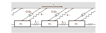
Abbildung 1: Diagram of the spring-slider-dashpot system. The configuration is identical to the Burridge-Knopoff model (Burridge and Knopoff, 1967), except that it is also equipped with dashpots and the friction on the bottom of the sliders is rate- and state-dependent.

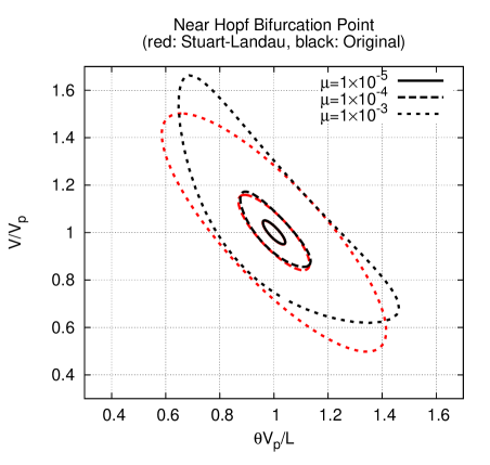
Abbildung 2: Periodic orbits of the Dieterich-Ruina oscillator near the bifurcation point, graphs of $\left(\theta V_{p}/L,V/V_{p}\right)$. Red and black curves are for the periodic solutions of the Stuart-Landau and original differential equations, respectively. The equilibrium point is $(1,1)$. The values of bifurcation parameter $\mu$ are set to $1\times 10^{-5}\mathrm{Nm^{-2}}$ (solid curves), $1\times 10^{-4}\mathrm{Nm^{-2}}$ (dashed curves), and $1\times 10^{-3}\mathrm{Nm^{-2}}$ (dotted curves). The values of $k$ used here are obtained by setting $k=(B-A-gV_{p}-\mu)/L$ and using the corresponding values of $\mu$. The rest of parameters are set to $(V_{p},g,A,B,L)=(3.17\times 10^{-9}\,\mathrm{ms^{-1}},\leavevmode\nobreak\ 5.00\times 10^{6}\,\mathrm{Nm^{-3}s},\leavevmode\nobreak\ 1.50\times 10^{5}\,\mathrm{Nm^{-2}},\leavevmode\nobreak\ 2.20\times 10^{5}\,\mathrm{Nm^{-2}},\leavevmode\nobreak\ 1.00\times 10^{-2}\,\mathrm{m})$.

Abbildung 3: A periodic orbit of the Dieterich-Ruina oscillator, a graph of $\left(\theta V_{p}/L,V/V_{p}\right)$, in a double logarithmic plane. The parameters are set to $(k,V_{p},g,A,B,L)=(1.00\times 10^{5}\,\mathrm{Nm^{-3}},\leavevmode\nobreak\ 3.17\times 10^{-9}\,\mathrm{ms^{-1}},\leavevmode\nobreak\ 5.00\times 10^{6}\,\mathrm{Nm^{-3}s},\leavevmode\nobreak\ 1.50\times 10^{5}\,\mathrm{Nm^{-2}},\leavevmode\nobreak\ 2.20\times 10^{5}\,\mathrm{Nm^{-2}},\leavevmode\nobreak\ 1.00\times 10^{-2}\,\mathrm{m})$. The equilibrium point is $(1,1)$.

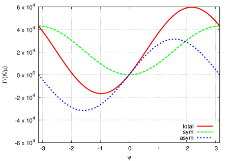
Abbildung 4: The phase coupling function as a function of phase, normalized by $\mu/k_{12}=\mu/k_{21}$ for a weakly nonlinear oscillator. The parameters are set to $(V_{p},g,A,B,L)=(3.17\times 10^{-9}\,\mathrm{ms^{-1}},\leavevmode\nobreak\ 5.00\times 10^{6}\,\mathrm{Nm^{-3}s},\leavevmode\nobreak\ 1.50\times 10^{5}\,\mathrm{Nm^{-2}},\leavevmode\nobreak\ 2.20\times 10^{5}\,\mathrm{Nm^{-2}},\leavevmode\nobreak\ 1.00\times 10^{-2}\,\mathrm{m})$. The blue, green, and red curves are the antisymmetric part defined by Eq. (53), symmetric part by Eq. (59), and total by Eq. (37), respectively.

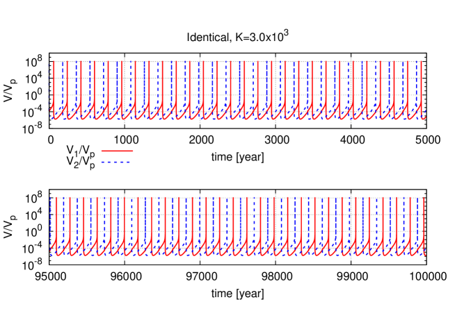
Abbildung 5: The time evolution of $V/V_{p}$ for case 0 in a logarithmic scale. The variation from $5000$ to $95000\mathrm{yr}$ is not shown. The parameters are $B=2.20\times 10^{5}\mathrm{Nm^{-2}}$ for both oscillators, and $K=3\times 10^{3}\mathrm{Nm^{-3}}$. The oscillators synchronize at a phase difference of $\psi=-3.14$ (anti-phase).

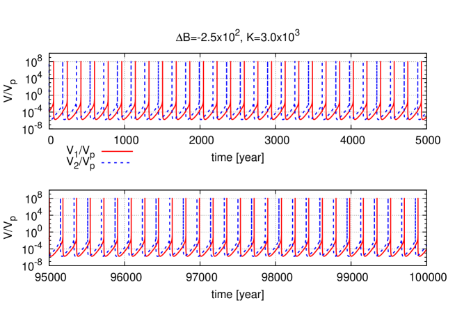
Abbildung 6: The time evolution of $V/V_{p}$ for case 1 in a logarithmic scale. The variation from $5000$ to $95000\mathrm{yr}$ is not shown. The parameters are $B=2.20\times 10^{5}\mathrm{Nm^{-2}}$ for oscillator 1, $B=2.2025\times 10^{5}\mathrm{Nm^{-2}}$ for oscillator 2, and $K=3\times 10^{3}\mathrm{Nm^{-3}}$. The oscillators synchronize at a phase difference of $\psi=-1.18$.

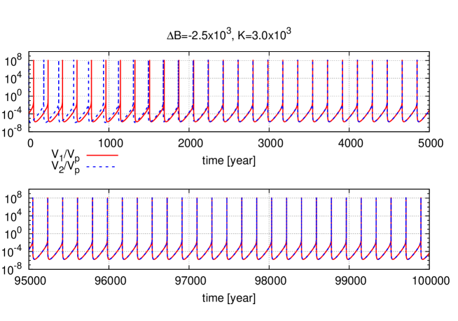
Abbildung 7: The time evolution of $V/V_{p}$ for case 2 in a logarithmic scale. The variation from $5000$ to $95000\mathrm{yr}$ is not shown. The parameters are $B=2.20\times 10^{5}\mathrm{Nm^{-2}}$ for oscillator 1, $B=2.225\times 10^{5}\mathrm{Nm^{-2}}$ for oscillator 2, and $K=3\times 10^{3}\mathrm{Nm^{-3}}$. The oscillators synchronize at a phase difference of $\psi=-7.07\times 10^{-3}$.

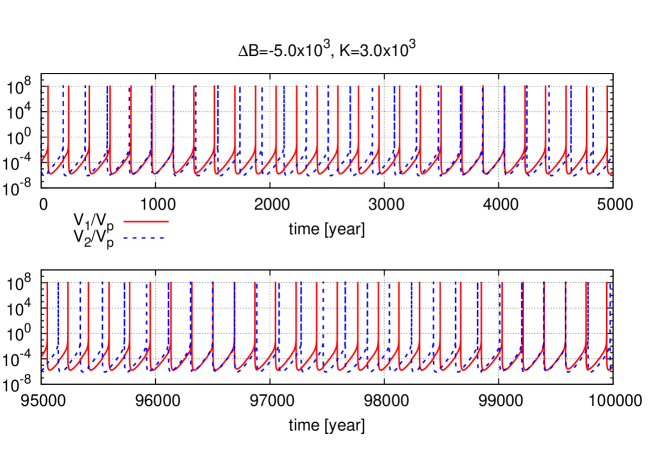
Abbildung 8: The time evolution of $V/V_{p}$ for case 3 in a logarithmic scale. The variation from $5000$ to $95000\mathrm{yr}$ is not shown. The parameters are $B=2.20\times 10^{5}\mathrm{Nm^{-2}}$ for oscillator 1, $B=2.25\times 10^{5}\mathrm{Nm^{-2}}$ for oscillator 2, and $K=3\times 10^{3}\mathrm{Nm^{-3}}$. The oscillators are not synchronized.

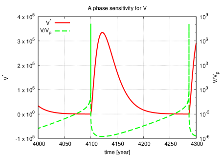
Abbildung 9: Phase sensitivity, $V^{*}$, as a function of time in years (red curve) calculated numerically using the relaxation method. The parameters are set to $(k,V_{p},g,A,B,L)=(1.00\times 10^{5}\,\mathrm{Nm^{-3}},\leavevmode\nobreak\ 3.17\times 10^{-9}\,\mathrm{ms^{-1}},\leavevmode\nobreak\ 5.00\times 10^{6}\,\mathrm{Nm^{-3}s},\leavevmode\nobreak\ 1.50\times 10^{5}\,\mathrm{Nm^{-2}},\leavevmode\nobreak\ 2.20\times 10^{5}\,\mathrm{Nm^{-2}},\leavevmode\nobreak\ 1.00\times 10^{-2}\,\mathrm{m})$. The green curve is for $V/V_{p}$ in a logarithmic scale. Note that $V^{*}$ becomes negative for some time periods in which $V/V_{p}$ is large.

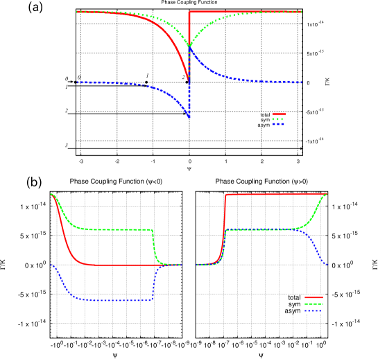
Abbildung 10: The phase coupling function, $\hat{\Gamma}$, as a function of phase, normalized by the coupling intensity $K=k_{12}=k_{21}$, in (a) linear scale of $\psi$ and (b) logarithmic scales of $\psi$. The parameters are set to $(k,V_{p},g,A,B,L)=(1.00\times 10^{5}\,\mathrm{Nm^{-3}},\leavevmode\nobreak\ 3.17\times 10^{-9}\,\mathrm{ms^{-1}},\leavevmode\nobreak\ 5.00\times 10^{6}\,\mathrm{Nm^{-3}s},\leavevmode\nobreak\ 1.50\times 10^{5}\,\mathrm{Nm^{-2}},\leavevmode\nobreak\ 2.20\times 10^{5}\,\mathrm{Nm^{-2}},\leavevmode\nobreak\ 1.00\times 10^{-2}\,\mathrm{m})$. The blue, green, and red curves are the antisymmetric part $\hat{\Gamma}_{a}$, symmetric part $\hat{\Gamma}_{s}$, and total $\hat{\Gamma}$, respectively. For each case in Table 1, the phase difference $\psi$ of synchronized oscillators and the corresponding value of $-\Delta\omega/(2K)$ are indicated by a filled circle and an arrow, respectively.

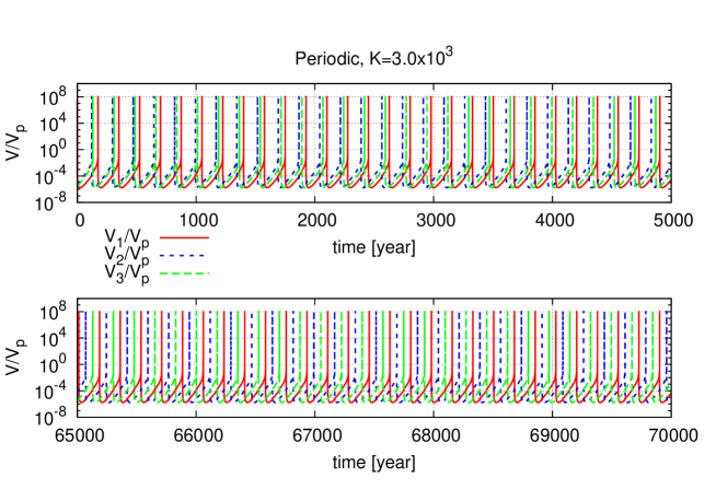
Abbildung 11: The time evolution of $V/V_{p}$ for three identical oscillators with a periodic coupling in a logarithmic scale. Red, blue, and green curves correspond to oscillator 1, 2, and 3, respectively. The variation from $5000$ to $65000\mathrm{yr}$ is not shown. The parameters are $B=2.20\times 10^{5}\mathrm{Nm^{-2}}$ for all oscillators, and $k_{12}=k_{23}=k_{31}=3\times 10^{3}\mathrm{Nm^{-3}}$ (periodic one-dimensional coupling). The three oscillators synchronize at the phase differences $(\psi_{1},\psi_{3})\simeq(\frac{2}{3}\pi,-\frac{2}{3}\pi)$. This synchronization corresponds to a stable spiral in Fig. 13.

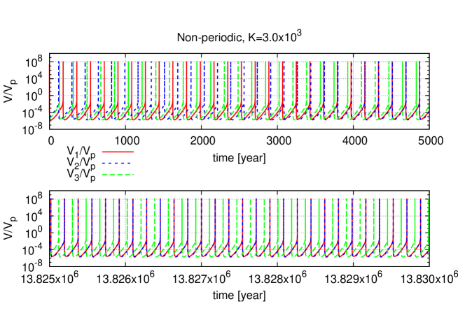
Abbildung 12: The time evolution of $V/V_{p}$ for three identical oscillators with a non-periodic one-dimensional coupling in a logarithmic scale. Red, blue, and green curves correspond to oscillator 1, 2, and 3, respectively. The variation from $5000$ to $13825000\mathrm{yr}$ is not shown. The initial states for three oscillators are different from each other. The parameters are $B=2.20\times 10^{5}\mathrm{Nm^{-2}}$ for all oscillators, and $k_{12}=k_{23}=3\times 10^{3}\mathrm{Nm^{-3}},k_{31}=0$ (non-periodic one-dimensional coupling). They synchronize at the phase differences of $(\psi_{1},\psi_{3})\simeq(7.0\times 10^{-3},2.6)$, where oscillators 1 and 2 are nearly in-phase. This synchronization corresponds to a stable node in Fig. 14.

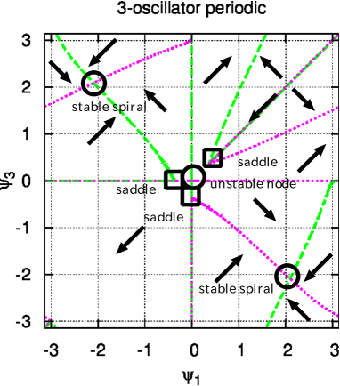
Abbildung 13: Flow directions and nullclines on the $(\psi_{1},\psi_{3})$-plane for the phase flow of three identical oscillators that are periodically coupled. Arrows indicate the flow direction. Green and red curves represent the nullcline $d\psi_{1}/dt=0$ and $d\psi_{3}/dt=0$, respectively. Stable spirals are located at $\left(\pm\frac{2}{3}\pi,\mp\frac{2}{3}\pi\right)$. The origin is an unstable node, and the three saddles are around $(0,-0.3)$,$(-0.3,0)$, and $(0.375,0.375)$.

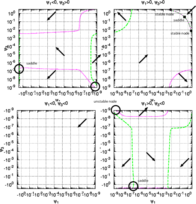
Abbildung 14: Flow direction and nullclines on the $(\psi_{1},\psi_{3})$-plane in a logarithmic scale for the phase flow of three identical oscillators that are non-periodically coupled. Arrows indicate the flow direction. Green and red curves represent the nullcline $d\psi_{1}/dt=0$ and $d\psi_{3}/dt=0$, respectively. Stable nodes are located around $\left(8\times 10^{-3},2.6\right)$ and $\left(2.6,8\times 10^{-3}\right)$. The origin is an unstable node, and saddles are around $(0.375,0.375)$, $(2\times 10^{-7},-3)$, and $(-3,2\times 10^{-7})$.

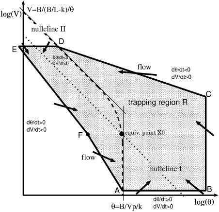
Abbildung 15: A trapping region in the $\log{\theta}$-$\log{V}$ plane. Dotted line represents nullcline I, dashed curve represents nullcline II, black dot is the equilibrium point $\vec{X}_{0}$, thick solid line represents a hexagon $H=ABCDEF$ that bounds the trapping region $R$, thin solid lines represent the asymptotes for nullcline II, and arrows represent the flows.

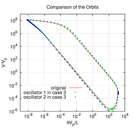
Abbildung 16: A comparison of the orbits, graphs of $\left(\theta V_{p}/L,V/V_{p}\right)$, in a double logarithmic plane. The red curve, green dots, and blue triangles are the orbits of the original limit cycle, oscillator 1 and 2 in case 3, respectively.

Tabelle 1: The synchronization properties of some pairs of coupled oscillators with different parameter settings. The corresponding values estimated from the PCF are shown in parentheses.

Case	0	1	2	3
$K$   $[\mathrm{Nm^{-3}}]$	$3.0\times 10^{3}$
$\Delta\omega$    $[\mathrm{s^{-1}}]$	0	$3.57\times 10^{-12}$	$3.47\times 10^{-11}$	$6.73\times 10^{-11}$
	(0)	($3.59\times 10^{-12}$)	($3.59\times 10^{-11}$)	($7.19\times 10^{-11}$)
$-\frac{\Delta\omega}{2K}$    $[\mathrm{kg^{-1}m^{2}s}]$	0	$-5.96\times 10^{-16}$	$-5.79\times 10^{-15}$	$-1.12\times 10^{-14}$
	(0)	($-5.99\times 10^{-16}$)	($-5.99\times 10^{-15}$)	($-1.19\times 10^{-14}$)
Synchronized?	Yes	Yes	Yes	No
	(Yes)	(Yes)	(Yes)	(No)
$\psi_{\mathrm{sync}}$	$-3.14$	$-1.18$	$-7.07\times 10^{-3}$	-
	($-3.14$)	($-1.23$)	($-7.53\times 10^{-3}$)	( - )
$\left.\frac{d\varphi}{dt}\right|_{\mathrm{sync}}-\overline{\omega}$    $[\mathrm{s^{-1}}]$	$3.62\times 10^{-11}$	$3.44\times 10^{-11}$	$1.76\times 10^{-11}$	-
	($3.61\times 10^{-11}$)	($3.44\times 10^{-11}$)	($1.81\times 10^{-11}$)	( - )