Hilbert-space localization in closed quantum systems

Abstract

Quantum localization within an energy-shell of a closed quantum system stands in contrast to the ergodic assumption of Boltzmann, and to the corresponding eigenstate thermalization hypothesis. The familiar case is the real-space Anderson localization and its many-body Fock-space version. We use the term Hilbert-space localization in order to emphasize the more general phase-space context. Specifically, we introduce a unifying picture that extends the semiclassical perspective of Heller, which relates the localization measure to the probability of return. We illustrate our approach by considering several systems of experimental interest, referring in particular to the Bosonic Josephson tunneling junction. We explore the dependence of the localization measure on the initial state, and on the strength of the many-body interactions using a novel recursive projection method.

I Introduction

For long time, the most important example of a complex finite quantum system was the atomic nuclei Blaizot_86 . Nowadays, there exist several other types of complex finite quantum systems that are experimentally accessible and widely studied, such as photon cavities, quantum dots, trapped atoms, metallic and magnetic nanoclusters, and graphene flakes cqed ; Walther_06 ; Lipparini_08 ; Pethick_08 ; Yukalov09 ; Katsnelson_12 ; Birman_13 . The existence of a variety of finite quantum systems opens a wide field for studying fundamental quantum properties. In recent years, high interest has been directed to the investigation of such interconnected problems as equilibration and thermalization PSSV_11 ; Yukalov_11 , and entanglement Williams_98 ; Nielsen_00 ; Vedral_02 ; Keyl_02 .

Random scattering in a quantum or classical wave-like system can cause a severe interference effect that creates a complex dynamics. While we expect diffusion in the presence of very weak random scattering, strong random scattering can lead to Anderson localization. In this case a particle cannot escape from a finite region, defined by the localization length. This picture was proposed in the seminal work of Anderson under the assumption that a single quantum particle is scattered in a static random environment anderson58 . A natural extension is a quantum gas, consisting of many particles. The description of such a system is substantially more complex, requiring a many-body wave function rather than a single-particle wave function in real space. The definition of localization is also different in the many-body system because the relevant space is the many-body Hilbert space rather than the real space of a single particle. On the other hand, a static random environment is not necessary to produce interference because interparticle scattering plays a similar role: An individual particle inside the quantum gas experiences scattering by other particles. Since the dynamics of the gas is quite complex, the scattering of an individual particle by other particles can be considered as random. Then the main difference in comparison to Anderson’s picture is that the scattering environment is dynamic rather than static. Thus, we expect that the motion of the many-body system is constraint to subregions in the Hilbert space by scattering events which cause strong interference of the many-body wave function. This will be called Hilbert-space localization subsequently, in contrast to Anderson localization. Our approach should be distinguished from other many-body generalizations, where the interplay of disorder and interactions was addressed Basko_06 ; gora ; Pal_10 ; Huse_13 .

The first work that placed the Quantum-localization theme in the context of finite complex systems concerns “the Standard Map”, aka “the Quantum Kicked Rotator model” QKRc . It has been realized QKRf that the observed localization can be mapped to the one-dimensional Anderson model with quasi-random disorder. Thus, the underlying “chaos” induces an effective disorder, but the localization is not in space but in momentum, hence termed dynamical localization. Subsequent studies have expanded this perspective. In particular we note the analysis of localization for coupled rotors TIPb , which has been motivated by the interest in getting a better understanding for the coherent propagation of interacting particles in random potential TIPs ; TIPb ; TIPi .

An important finding of Borgonovi and Shepelyansky TIPb is the enhancement of the localization length for two kicked rotators, as compared to the length of a single kicked rotator. This result suggests that particle interactions can induce an increased localization length or even delocalization of otherwise localized single noninteracting particles, although in many other cases, particle interactions strengthen localization Kramer . Thus, interaction can produce both effects of either strengthening, weakening or even destroying localization. Another examples are cold atoms, where Anderson localization of noninteracting atoms in random or quasiperiodic optical lattices can be destroyed by atomic interactions (see review Modugno ).

Generally speaking, the role of interactions is not as simple, and they can produce both effects, either enhancing localization or destroying it. Their influence depends on details of the considered physical system, including Bose or Fermi statistics, the peculiarity of the energy spectrum, the specifics of the interaction forces, whether the latter are short-ranged or long-ranged, repulsive or attractive, and thermodynamic characteristics, such as temperature or pressure, also play their role.

We would like to point out that in a small complex system, disorder is in general not a relevant notion, and the localization effect can depend in a non-monotonic way on the strength of the interactions. A minimal example for that is the observed localization in the 4 site Bose-Hubbard model ckt . What matter are the characteristics of the phase-space structure. The interplay between disorder and interaction becomes an issue if one considers larger clusters, still the same framework should handle all cases on equal footing.

In the present paper we address the question of quantum localization from a more general point of view. Using the term Hilbert-space localization (HSL) we want to make clear that quantum localization does not have to show up in a particular dynamical variable. Our perspective is motivated by the work of Heller Heller_87 regarding the semiclassical picture of weak localization in phase-space, aka “scarr theory”. Here we extend this perspective and use it to discuss strong localization, irrespective of whether it originates from disorder or from interactions between particles, and irrespective of whether it is in “position” or in “momentum”.

The outline of the paper is as follows. In section II, we distinguish between two notions of phase-space exploration. This allows for a generalized definition of quantum breaktime in sections III and  IV, which is the reason for having quantum localization. In Section V, we discuss the calculation of the localization measure, while in Section VI, we illustrate the procedure with regard to the Bosonic Josephson junction. For completeness, the traditional notion of spatial localization and its related entropy-based measures are briefly summarized in Appendix A and in the Appendix B. The other appendices contain models-related material that has not been included in the main text.

II Exploration of phase-space

In “Quantum localization and the rate of exploration of phase space” Heller_87 Heller has provided a semiclassical perspective for quantum localization of eigenstates. His framework was effective for the discussion of weak localization and scarring, while the strong localization effect, as well as the many-body localization theme, were left out of the semiclassical framework. We would like to refine the phase-space semiclassical framework in order to achieve a more comprehensive heuristic understanding of quantum localization. This proposed extension incorporates the dynamical breaktime concept (see dittrich ; brk and further references therein) that had been introduced in order to shed light on the strong Anderson localization effect in ${d=1,2,3}$ dimensions. Our starting point is a distinction between two different notions of participation numbers:

$$\mathcal{N}_{\text{cells}}(t) = \mbox{\#explored ``cells" at time~{}$t$}\;,$$

$$\mathcal{N}_{\text{states}}(t) = \mbox{\#participating states up to time~{}$t$}\;.$$

We shall define these two functions below. Schematic illustration of them in the case of a diffusive-like system is provided in Fig. 1. For the purpose of the present section, it is useful to have in mind a simpler example: the free expansion of a wavefunction is a chaotic ballistic (non diffusive) billiard. The initial state is a Gaussian wavepacket. Two energy scales are involved:

$$\Delta_{0}= \equiv\ {2\pi\hbar}/{t_{H}}$$ mean level spacing (1)

$$\Delta_{E}= \equiv\ {2\pi\hbar}/{\tau_{E}}\;,$$ energy shell width (2)

where we have defined corresponding time scales $t_{H}$ (Heisenberg time) and $\tau_{E}$ (uncertainty time). The width of the energy shell is determined by the energy uncertainty of the preparation. The effective Hilbert space dimension is

$$\mathcal{N}_{E}\ \ =\ \ \frac{\Delta_{E}}{\Delta_{0}}\;.$$ (3)

Without loss of generality, and for presentation clarity, we assume that all the out-of-shell states have been truncated and, hence, we regard $\mathcal{N}_{E}$ as the actual Hilbert space dimension. It follows that any “participation number” $\mathcal{N}$ is a-priori bounded by the value $\mathcal{N}_{E}$.

Given an arbitrary statistical state $\rho$, the number of participating (pure) states $\mathcal{N}\equiv\exp[\mathcal{S}]$ can be defined either via the Shanon entropy $\mathcal{S}=-\mbox{Trace}[\rho\ln\rho]$, or via $\mathcal{N}=1/\mbox{Trace}[\rho^{2}]$, or more generally via the Renyi entropy which involves $\mbox{Trace}[\rho^{\gamma}]$, see App.B for definitions. An initial Gaussian wavepacket preparation ${\rho=|\psi\rangle\langle\psi|}$, as well as the evolved state ${\rho=|\psi(t)\rangle\langle\psi(t)|}$, have zero entropy, meaning that the number of participating states in any instant of time is $\mathcal{N}(t)=1$. We now turn to explain the definitions of $\mathcal{N}_{\text{cells}}(t)$ following Boltzmann, and of $\mathcal{N}_{\text{states}}(t)$ following Heller.

The procedure of Boltzmann is to divide phase space into cells. In the quantum version, one can define a corresponding partitioning of Hilbert space using a complete set of projectors $\hat{P}_{n}=|n\rangle\langle n|$. Then, from the coarse-grained distribution ${p_{n}}$, using any of the above Renyi measures, one can define the number of explored “cells” $\mathcal{N}_{\text{cells}}(t)$. We shall prefer below to use the $\mbox{Trace}[\rho^{2}]$ based definition, Namely,

$$\mathcal{N}_{\text{cells}}(t)\ =\ \left[\sum p_{n}^{2}\right]^{-1},$$ (4)

$$\ \ \ \text{where}\ \ \ p_{n}(t)=\left|\left\langle n\middle|\psi(t)\right\rangle\right|^{2}\;.$$ (5)

Following Heller, we define also $\mathcal{N}_{\text{states}}(t)$, which was described in Heller_87 as the “number of phase-space cells accessed”. We prefer the term “number of participating states up to time $t$”. We shall see in a moment that the semantics is important. The definition of $\mathcal{N}_{\text{states}}(t)$ is based not on the coarse grained $\rho$ at time $t$, but rather on the time-averaged $\rho$ during the time interval ${[0,t]}$. Namely,

$$\mathcal{N}_{\text{states}}(t) = \mbox{Trace}\left[\left(\frac{1}{t}\int_{0}^{t}\rho(t^{\prime})dt^{\prime}\right)^{2}\right]^{-1}$$ (6)

$$= \left[\frac{2}{t}\int_{0}^{t}\left(1-\frac{\tau}{t}\right)\mathcal{P}(\tau)d\tau\right]^{-1}\;.$$ (7)

The last equality relates $\mathcal{N}_{\text{states}}(t)$ to the survival probability. The latter is defined as follows:

$$\mathcal{P}(t)\ =\ \left|\left\langle\psi(0)\middle|\psi(t)\right\rangle\right|^{2}\ =\ \sum_{\alpha,\beta}p_{\alpha}p_{\beta}\,e^{i(E_{\beta}-E_{\alpha})t},\ \ \$$ (8)

$$\ \ \ \text{where}\ \ \ p_{\alpha}=\left|\left\langle E_{\alpha}\middle|\psi\right\rangle\right|^{2}\;.$$ (9)

The function $\mathcal{N}_{\text{states}}(t)$ provides the size of the basis that is required in order to simulate the dynamics up to time $t$. It is a-priori bounded by the value $\mathcal{N}_{E}$. Its asymptotic value is

$$\mathcal{N}_{\infty}\ =\ \mathcal{N}_{\text{states}}(\infty)\ =\ \left[\overline{\mathcal{P}(t)}\right]^{-1}$$ (10)

where the overline indicated time averaging. For a non-degenerate spectrum it follows that

$$\mathcal{N}_{\infty}\ =\ \left[\sum p_{\alpha}^{2}\right]^{-1}$$ (11)

This is known as the participation number (PN) of eigenstates. The function $\mathcal{N}_{\text{states}}(t)$ can be regarded as a time-dependent generalization of the conventional PN notion.

III The localization measure

The concept of spatial localization can be adopted to more complex quantum systems Heller_87 ; Logan_90 by considering a general basis of states $\{|n\rangle\}$ that define “locations” within the energy shell. Then the evolution starts with an initial state $|\psi\rangle$ and evolves in time as ${|\psi(t)\rangle=\exp(-i\mathcal{H}t)|\psi\rangle}$. It can be understood as a walk in the Hilbert space, where we expect that all states are visited with some probability. An important point is that the general form of the transition probability

$$P_{t}(n^{\prime}|n)\ \ =\ \ |\langle n^{\prime}|e^{-i\mathcal{H}t}|n\rangle|^{2}$$ (12)

depends on $n$ and $n^{\prime}$ separately, whereas the spatial transition probability, characterizing spatial localization (see App.A), depends only on the difference $|r^{\prime}-r|$. This is a consequence of the translational invariance in real space after disorder averaging. It follows that both $\mathcal{P}(t)$ and $\mathcal{N}_{\text{states}}(t)$, as well as the asymptotic value $\mathcal{N}_{\infty}$ dependent in general on the initial state $|\psi\rangle$. Let us re-write Eq. (10) in a way that emphasize this point:

$$\mathcal{N}_{\infty}^{-1}\ =\ \lim_{\epsilon\to 0}\epsilon\int_{0}^{\infty}|\langle\psi|e^{-i\mathcal{H}t}|\psi\rangle|^{2}e^{-\epsilon t}dt\;.$$ (13)

The dependence on the initial state $\psi$ becomes obvious when we choose it to be an eigenstate $\left|E_{\alpha}\right\rangle$ of $\mathcal{H}$, which gives $\mathcal{N}_{\infty}=1$. In this case, the system remains in the initial state for all times. An initial state $\left|n_{0}\right\rangle$ within the energy-shell might be similar to an eigenstate of $\mathcal{H}$. Then the question is whether it will visit only a fraction or the entire Hilbert space. From the definition Eq. (10) and the spectral decomposition Eq. (8) it follows that

$$\mathcal{N}_{\infty}^{-1}\ =\ \lim_{\epsilon\to 0}\epsilon^{2}\sum_{\alpha,\beta}\frac{p_{\alpha}p_{\beta}}{\epsilon^{2}+(E_{\alpha}-E_{\beta})^{2}}\;.$$ (14)

For a non-degenerate discrete spectrum we obtain Eq. (11), and hence identify $\mathcal{N}_{\infty}$ as the number of participating eigenstates. Recall that $\mathcal{N}_{E}$ is the effective Hilbert space dimension. Accordingly, the following ratio can be used as a measure for localization Heller_87 :

$$\mathcal{F}\ \ =\ \ \frac{\mathcal{N}_{\infty}}{\mathcal{N}_{E}}\;.$$ (15)

It is the fraction of eigenstates within the energy shell that participate in the dynamics, and by Eq. (10) it is also the fraction of cells that will be occupied by the probability distribution in the long time limit. It is implicitly assumed that the preparation $\psi$ is localized in a small region of the energy shell, as in the case of a Gaussian wavepacket in a chaotic billiard. The dimension of Hilbert space $\mathcal{N}_{E}$ is proportional to the volume, while $\mathcal{N}_{\infty}$ would be volume-independent if the eigenstates were localized. Accordingly a vanishingly small $\mathcal{F}$ constitutes an indication for a strong quantum localization effect.

In a practical calculation, it is essential to use consistent mathematical definitions for $\mathcal{N}_{E}$ and $\mathcal{N}_{\infty}$. It is convenient to express them in terms of a the smoothed spectral density, the so called local density of states,

$$\varrho_{\epsilon}(\omega)\ = \ \frac{1}{\pi}\mbox{Im}\left\langle\psi\middle|(\omega-i\epsilon-\mathcal{H})^{-1}\middle|\psi\right\rangle$$ (16)

$$= \left\langle\psi\middle|\delta(\omega-\mathcal{H})\middle|\psi\right\rangle\;.$$ (17)

The survival probability $\mathcal{P}(t)$ is the squared absolute value of its Fourier transform, while for the participation number we get

$$\mathcal{N}_{\infty}^{-1}\ =\ 2\pi\lim_{\epsilon\to 0}\epsilon\int[\varrho_{\epsilon}(\omega)]^{2}d\omega\;.$$ (18)

The right-hand-side can be treated within the recursive projection method ziegler03 ; ziegler11 , see Sec.VI. On equal footing, we can define the effective Hilbert space dimension from a semiclassical calculation:

$$\mathcal{N}_{E}^{-1}\ =\ 2\pi\int[\varrho_{\text{cl}}(\omega)]^{2}d\omega\;.$$ (19)

In the absence of a classical limit $\varrho_{\text{cl}}(\omega)$ can be regarded as the envelope of $\varrho_{\epsilon}(\omega)$.

IV Quantum ergodization

The simplest dynamical scenario of ergodization concerns a fully-chaotic Sinai billiard. The function $\mathcal{N}_{\text{cells}}(t)$ approaches the saturation value $\sim\mathcal{N}_{E}$ after a very short ergodic time $t_{\text{erg}}$ that is determined by the curvature of the walls. Similarly, the function $\mathcal{N}_{\text{states}}(t)$ approaches the asymptotic value $\mathcal{N}_{\infty}=\mathcal{N}_{E}$ in the classical case, or $\mathcal{N}_{\infty}=\mathcal{N}_{E}/3$ in the quantum case. The factor ${\mathcal{F}_{\text{RMT}}=1/3}$ reflects the Gaussian statistics of a random-wave amplitude. Not all possible preparations look like random waves. If we start a wavepacket at the vicinity of an unstable periodic orbit, $\mathcal{F}$ might be further suppressed due to recurrences. The suppression factor depends on the Lyapunov instability exponent $\lambda$, and is given by a variation of a formula of the following type scar1 ; scar2 :

$$\mathcal{F}\ \ \approx\ \ \left[\sum_{s=-\infty}^{\infty}\frac{1}{\cosh(\lambda s)}\right]^{-1}\mathcal{F}_{\text{RMT}}\;.$$ (20)

The study of a periodically kicked Bosonic Joshephson Junction provides a nice demonstration for this formula ckt . One should regard “scarring” as a weak localization effect.

Let us describe how $\mathcal{N}_{\text{states}}(t)$ looks like in the absence of strong localization effect. We still have in mind the simplest dynamical scenario of ergodization that concerns a fully-chaotic Sinai billiard. This function differs from $\mathcal{N}_{\text{cells}}(t)$ because the time-averaged $\rho(t)$ gives a large weight to the initial preparation, which diminishes only algebraically (as $1/t$) in the ${t\rightarrow\infty}$ limit. To make this point clear, notice that the survival probability $\mathcal{P}(t)$ decays within a time $\tau_{E}$. For short times it is roughly described by recurrences-free quantum exploration function

$$\mathcal{N}^{(0)}_{\text{states}}(t)\ \ =\ \ \frac{t}{\tau_{E}}\;.$$ (21)

After that, there are recurrences whose long time average saturates asymptotically to the value $1/\mathcal{N}_{\infty}$. Therefore we get roughly

$$\mathcal{N}_{\text{states}}(t)\ \ \approx\ \ \left[\frac{1}{t/\tau_{E}}+\frac{1}{\mathcal{N}_{\infty}}\right]^{-1}\;.$$ (22)

This expression is characterized by a crossover time that we call “quantum breaktime”. In the present example we identify the quantum breaktime with the Heisenberg time, namely,

$$t^{*}[\text{for ergodic system}]\ \ \sim\ \ \mathcal{N}_{\infty}\tau_{E}\ \ \sim\ \ t_{H}\ .$$ (23)

We conclude that in the simple quantum ergodization scenario the two functions $\mathcal{N}_{\text{cells}}(t)$ and $\mathcal{N}_{\text{states}}(t)$ involve completely different time scales. The former get ergodized after a short classical time $t_{\text{erg}}$, while the latter saturates only after the quantum Heisenberg time $t_{H}$. This picture changes completely if we have a strong localization effect, as discussed in the next section.

In more complicated systems, there are two types of modifications that are expected in Eq. (22). Weak localization corrections (scar-theory related) can be deduced from the study of the survival probability. Recall that $\mathcal{P}(t)$ is determined by the Fourier transform of the local density of states $\varrho(\omega)$. The short time behavior reflects the envelope of this spectral function, while for longer times a power law decay $\mathcal{P}(t)\sim t^{-\gamma}$ would reflect the fractal dimension of the participating eigenstates lea1 ; lea2 . Accordingly,

$$\mathcal{N}_{\text{states}}(t)\ \ \sim\ \ \left[\frac{\text{const}}{t^{\gamma}}+\frac{1}{\mathcal{N}_{\infty}}\right]^{-1}\;.$$ (24)

By definition, the asymptotic value $\mathcal{N}_{\infty}$ reflects the number of participating eigenstates, and can be deduced semiclassically too. This will be discussed in the following sections. We refer to the possibility of having ${\mathcal{N}_{\infty}\ll\mathcal{N}_{E}}$ as a strong localization effect.

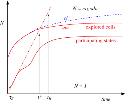
Figure 1: Schematic description for the exploration of phase-space versus time. For example it might be the phase-space of billiard that consists of connected-boxes (see text). Diffusion-like dynamics is assumed. The participation number is bounded between the minimal value $\mathcal{N}=1$ and the maximal ergodic value $\mathcal{N}_{E}$, which are represented by horizontal dotted lines. The upper dashed and solid lines are the Boltzmann exploration function $\mathcal{N}_{\text{cells}}(t)$ in the classical and in the quantum evolution, respectively. They depart at the breaktime $t^{*}$, and consequently a quantum localization effect manifests itself. The lower solid and dashed lines are $\mathcal{N}_{\text{states}}(t)$ and its upper bound $\mathcal{N}_{\text{states}}^{(0)}(t)$, respectively. The former reflects the survival probability, while the latter is determined by the width of the energy-shell and intersects $\mathcal{N}_{E}$ at the Heisenberg time $t_{H}$. The actual breaktime $t^{*}$ is determined by the intersection with $\mathcal{N}_{\text{cells}}(t)$. Quantum localization is implied if $t^{*}<t_{H}$. If the dynamics were fully chaotic as for Sinai billiard, then $\mathcal{N}_{\text{cells}}(t)$ would reach the ergodic limit almost immediately, and consequently we would have $t^{*}\sim t_{H}$ implying no localization. In the absence of recurrences $\mathcal{N}_{\text{states}}(t)\sim\mathcal{N}_{\text{states}}^{(0)}(t)$ implying full quantum-ergodization without even a weak localization effect.

V Strong localization

Strong localization means that the breaktime $t^{*}$ is shorter than the Heisenberg time $t_{H}$. The prototype example is of course Anderson localization where the breaktime is related to the strength of the disorder and not to the total volume of the system, leading to a finite localization length in space. Here we would like to formulate the notion of “strong localization” in a more general way, within the HSL phase-space framework.

If we have a strong quantum-localization effect the role of $t_{\text{erg}}$ and $t_{H}$ is taken by the quantum breaktime $t^{*}$, as illustrated in Fig. 1. For presentation purpose we still consider a variant of the Anderson model: an array of connected chaotic boxes, with a particle that can migrate from box to box via small holes. In such a scenario, the classical exploration of phase-space is slow, diffusive-like. This means that $t_{\text{erg}}$ is very large, and can be defined as the time that it takes to diffuse over the whole volume of the array. The basic conjecture is that quantum-to-classical correspondence (QCC) is maintained as long as $t$ is smaller than the running Heisenberg time. The latter refers, by definition, not to the total volume but to the explored volume. Accordingly, the necessary condition for QCC is ${t\ll[\mathcal{N}_{\text{cells}}(t)/\mathcal{N}_{E}]t_{H}}$. This can be re-written as ${\mathcal{N}^{(0)}_{\text{states}}(t)\ll\mathcal{N}_{\text{cells}}(t)}$. Using a classical estimate for the number of explored cells, we deduce a more practical version for this condition:

$$\mathcal{N}^{(0)}_{\text{states}}(t)\ \ll\ \mathcal{N}^{cl}_{\text{cells}}(t),\ \ \ \ \ \ \ \ \text{[QCC condition]}\;.$$ (25)

Clearly, for diffusive-like dynamics, the breakdown of this inequality might happen before the ergodic time as illustrated in Fig. 1. Under such circumstances strong quantum localization is expected.

The reasoning above is not rigorous, still it provides the correct predictions as far as Anderson localization is concerned, and we believe that it can be trusted in more general circumstances (see below). It offers an illuminating semi-classical alternative to the formal Anderson criterion anderson58 . Note that the use of the Anderson criterion is restricted to disordered lattices that have well defined “connectivity”, while semiclassics can take into account the implications of complex phase-space structures.

The semiclassical localization criterion determines whether strong localization effect is expected, and provides a practical estimate for the localization volume. The procedure is simple: Given a dynamical system we have to find $\mathcal{N}^{cl}_{\text{cells}}(t)$. Then we estimate $t^{*}$ as the time when Eq. (25) breaks down, and the localization volume as $\mathcal{N}^{cl}_{\text{cells}}(t^{*})$. We can further conjecture that the saturation value $\mathcal{N}_{\infty}$ is of the same order of magnitude (“one parameter scaling”). The implicit assumption in this procedure is that the localization effect correlates the functions $\mathcal{N}_{\text{cells}}(t)$ and $\mathcal{N}_{\text{states}}(t)$, as illustrated in Fig. 1.

In a diffusive system, the classical exploration grows asymptotically like $t^{1/2}$ in 1D, like $t/\ln(t)$ in 2D, and like $t$, with small corrections, for higher dimensions brk . Schematically, we write

$$\mathcal{N}^{cl}_{\text{cells}}(t)\ \sim\ \text{const}\ +\ g\times\left(\frac{t}{\tau_{E}}\right)^{\alpha}\;.$$ (26)

From Eq. (25) we deduce that for sub-linear time dependence (${\alpha<1}$), we always have quantum localization, as in the case of diffusion in 1D/2D. On the other hand, if the asymptotic rate of exploration is linear (${\alpha=1}$), then the prefactor $g$ becomes important: the condition for quantum localization becomes ${g<1}$, implying a mobility edge. For a diffusive particle in a $d$-dimensional array of connected-boxes, one can easily show that ${g=(k\ell)^{d-1}(\ell/L)}$, where $k$ is the wavenumber, $\ell$ is the linear size of each box, and $L$ is the mean free path for box-to-box migration.

More generally, in quantized chaotic systems, the exploration of phase space can be slowed down by cantori (remnants of Kolmogorov-Arnold-Moser tori) or due to the sparsity of the Arnold web. Turning to the many body localization problem, a mobility edge is implied in any dimension, provided the classical rate of exploration depends on energy, such that above some $E_{c}$ the exploration is linear in time and fast enough. For any system with more than two degrees of freedom, the resonances between the coupled degrees of freedom form an “Arnold web” in phase-space. As energy is increased, the competition is between the width of the filaments and their density. Typically, above some critical energy the filaments overlap and we get fast exploration – this is called Chirikov criterion. But also, below this critical energy there is spreading which is called “Arnold diffusion”. Thus one expects in the latter case quantum localization too ArQ1 ; ArQ2 .

An interesting application of the above framework is in order to determine the criterion for superfluidity in atomtronic circuits. It has been demonstrated numerically sfc that superfluidity can be dynamically stable in rings that are described by the Bose-Hubbard Hamiltonian. The explanation of this stability requires “quantum localization” in a region where the Arnold diffusion prevails.

VI The recursive projection method

In principle, the participation number $\mathcal{N}_{\infty}$ can be determined numerically, provided the total dimension of Hilbert space is not too large. But if we want analytical results, we have to adopt an appropriate method. One possibility is to use semiclassics. The leading order semiclassics is merely the calculation of phase space-volumes, and hence can provide us $\mathcal{N}_{E}$. But then we have to adopt higher order semiclassics (periodic orbit theory or RMT phenomenology) in order to say anything regarding $\mathcal{F}$. If we want to get results for strong localization, we have to use complicated summation methods, or to be satisfied with the breaktime phenomenology.

In the next section, we would like to demonstrate an exact calculation of $\mathcal{N}_{\infty}$ using the recursive projection method (RPM). Given an initial state $|\psi\rangle$, this method facilitates the calculation of the return amplitude. A Laplace transformation ${t\to z}$ maps the evolution operator to the resolvent $(z-H)^{-1}$, while the inverse mapping is provided by a Cauchy integration on the complex $z$-plane. The advantage of using the resolvent is its presentation as a rational function with polynomials $Q_{N}(z)$ and $P_{N-1}(z)$:

$$G_{0}(z)\ =\ \langle\psi|(z-H)^{-1}|\psi\rangle=\frac{P_{N-1}(z)}{Q_{N}(z)}\ .$$ (27)

Its poles of $G_{0}(z)$ are determined by the the zeros of $Q_{N}(z)$, and they are the eigenvalues of $H$. The RPM provides an efficient procedure to calculate these polynomials. Starting from the fact that the resolvent can be expanded in powers of $H$, the resulting geometric series can be understood as a random walk in Hilbert space, where each sub-Hilbert space is visited an arbitrary number of times. In general, this series, also known as the Neumann series of the resolvent, has an infinite number of terms and is valid only within its radius of convergence. The main idea of the RPM is to re-organize the geometric series as a directed random walk through the $N$-dimensional Hilbert space, where each sub-Hilbert space is visited only once ziegler03 ; ziegler11 , rather than an arbitrary number of times.

Following the recipe described in Ref. ziegler11 , we obtain the rational function Eq. (27) in $N$ calculational steps. Since this still gives quite lengthy expressions for the polynomials with typical values $N=30...50$, we plot only the resulting values of the return probability as a function of time and $\mathcal{N}_{\infty}$ as a function of $N$ here.

VII Bosonic Josephson Junction

Small closed systems have the advantage that: (i) they can be realized experimentally and (ii) theoretical calculations are simple and in many cases can be performed exactly for finite dimension $N$. Prominent examples are the Jaynes-Cummings model jaynes63 ; cummings65 , which describes the interaction of a two-level system in an optical cavity (cf. App.C), coupled photon cavities cqed , and Josephson tunneling junctions for bosonic atoms in a double well potential milburn97 ; ketterle04 ; oberthaler05 ; Boukobza ; gati06 ; oberthaler07 ; cohen10 . Interacting bosons in a double-well potential are described in a two-mode approximation by the Bose-Hubbard Hamiltonian oberthaler07 :

$$\mathcal{H}_{\text{BH}}=\frac{U}{2}\sum_{j=1}^{2}a_{j}^{{\dagger}}a_{j}^{{\dagger}}a_{j}a_{j}-\frac{J}{2}\left(a_{2}^{{\dagger}}a_{1}+\text{h.c.}\right)\ ,$$ (28)

where $a_{j}$ and $a_{j}^{\dagger}$ are the bosonic annihilation and creation operators of the two wells, respectively. This Hamiltonian acts on the space that is spanned by the Fock basis $\{|N-k,k\rangle\}_{0\leq k\leq N}$, where

$$\left|n\right\rangle\ \ \equiv\ \ |N-n,n\rangle\ \ \equiv\ \ |N-n\rangle\otimes|n\rangle$$ (29)

is the state with $N-n$ bosons in the left well and $n$ bosons in the right well. The first term of the Hamiltonian describes a local interaction of the bosons, enforcing a symmetric distribution in the double well for $U>0$, while the second term of $\mathcal{H}_{\text{BH}}$ describes tunneling of bosons between the wells. As a characteristic dimensionless parameter of the Bose-Hubbard Hamiltonian we employ

$$u\ \ =\ \ \frac{NU}{J}\ ,$$ (30)

which is the ratio of the interaction energy over the tunneling energy. The factor $N$ takes care of the fact that the interaction energy grows like $N^{2}$ in our model, while the tunneling energy grows like $N$.

VII.1 Limiting cases

We first consider two limiting cases for the bosonic Josephson junction: (i) the $J{=}0$ case; (ii) the $U{=}0$ case. The latter describes e.g. photons in two coupled cavities. The transition probability in case (i) is

$$|\langle N-n,n|e^{-iHt}|N-n,n\rangle|^{2}\ =\ 1\;,$$ (31)

which implies $\mathcal{N}_{\infty}=1$ and describes a trivial case of HSL. For case (ii), a simple calculation reveals for the return amplitude cqed ; ziegler11

$$\langle N,0|e^{-iHt}|N,0\rangle\ =\ \cos^{N}(Jt/2)\;,$$ (32)

when the initial state has all $N$ bosons in one well. Thus the evolution in the Fock state is periodic with period $2\pi/J$. For $N=1$, we get $\mathcal{N}_{\infty}=2$, while for $N\gg 1$, using the Stirling formula (see App.E), we obtain

$$\mathcal{N}_{\infty}\sim\sqrt{\pi N/2}\ ,$$ (33)

which clearly indicates the absence of HSL, as we would have anticipated for independent bosons.

The most interesting question is what happens if $J,U\neq 0$; i.e., when tunneling and interaction compete. This can be addressed either in a mean-field approximation, in a semiclassical calculation, or by an exact solution of the quantum dynamics, using the recursive projection method for $\mathcal{N}_{\infty}$ in Eq. (18).

VII.2 Pendulum analogy

It is natural to consider first the simplest possible approximation. The prototype one-degree of freedom system is the pendulum. The Josephson junction is described formally by the same Hamiltonian with conjugate action-angle canonical coordinates ${(\varphi,n)}$, and with $\hbar\rightarrow(E_{C}/E_{J})^{1/2}$. The Bosonic Josephson junction (”dimer”) is a different version of the pendulum Hamiltonian with $\hbar\rightarrow 1/N$, where $N$ is the number of particles. Our calculation below refers to the latter, therefore we highlight the $N$ dependence of the results.

Let us summarize a few known results that concern the dimer ckt : (1) For a ground-state preparation $\mathcal{N}_{\infty}$ is of order unity. (2) For a preparation at the vicinity of the hyperbolic classically-unstable point $\mathcal{N}_{\infty}\sim\log(N)$. (3) For a generic preparation $\mathcal{N}_{\infty}\sim N^{1/2}$. The latter is implied by the uncertainty relation $\Delta\varphi\Delta n\sim\hbar\rightarrow 1/N$. (4) For a periodically driven chaotic dimer $\mathcal{N}_{\infty}\sim N$, with scar-theory correction Eq. (20) in the vicinity of unstable periodic periods.

VII.3 Mean-field dynamics

We consider the initial preparation ${\left|N,0\right\rangle}$. Then the expectation values for the number of bosons in the left well at time $t$ is

$$N_{1}(t) = \langle\psi(t)|a_{1}^{\dagger}a_{1}|\psi(t)\rangle$$ (34)

$$= \langle\psi(0)|e^{iHt}a_{1}^{\dagger}a_{1}e^{-iHt}|\psi(0)\rangle\ .$$ (35)

For this quantity, a mean field approximation exists in the form of a nonlinear Schrödinger (Gross-Pitaevskii) equation milburn97 ; eilbeck85 . The solution reads

$$N_{1}(t) = \frac{N}{2}\left[1+\mbox{cn}(2Jt|N^{2}/N_{c}^{2})\right],$$ (36)

$$N_{c} = \frac{2N}{u}=\frac{2J}{U}$$ (37)

with the initial value $N_{1}(0)=N$. The Jacobian elliptic function $\mbox{cn}(x|y)$ abramowitz is periodic in the first argument for $y\neq 1$ and changes its behavior qualitatively when the second argument $y=(u/2)^{2}$ crosses over from $y<1$ to $y>1$. The corresponding spectrum is equidistant, with $E_{k}=(2k+1)\pi J/K(u^{2}/4)$, where $K(m)$ is the integral

$$K(m)=\int_{0}^{\pi/2}\frac{1}{\sqrt{1-m\sin^{2}\phi}}d\phi\ .$$

Two examples for $N_{1}(t)$ are depicted in Fig. 2. In terms of our bosonic double well system, the behavior for ${N<N_{c}}$ describes unhindered tunneling of the bosons from one well to the other, whereas for ${N>N_{c}}$, only a fraction of the bosons are allowed to tunnel. This behavior is known as self-trapping milburn97 ; eilbeck85 or mode-locking YYB_97 ; YYB_00 ; YYB_02 and reminds us of HSL, since it indicates that the bosons are trapped in the well from which the particle dynamics started originally, and it cannot explore the entire Hilbert space spanned by $\{\left|n\right\rangle\}$.

Figure 2: Mean field dynamics of the boson density $N_{1}(t)/N$ in the left well, as described in Eq. (36). The function $[1+\mbox{cn}(t|y)]/2$ is plotted for different values of $y$, namely $y=0.8$ (full curve) and $y=1.1$ (dashed curve). Axes units are dimensionless.

VII.4 Semiclassical dynamics

The two-site Bose-Hubbard Hamiltonian for $N$ bosons is equivalent to a nonlinear $SU(2)$ spin model in $N+1$ dimensions (cf. App.D)

$$H_{S}\ =\ UL_{z}^{2}-JL_{x}\ .$$ (38)

Thus the semiclassical dynamics can be represented in a spherical phase-space. The expectation values of ${(L_{x},L_{y},L_{z})}$ are known as the Bloch vector. In order to visualize a wavefunction, the Bloch vector is not sufficient: we have to think about the Wigner function $\rho_{W}(\theta,\varphi)$. For coherent-state preparation, the Wigner function looks like a minimal Gaussian. In the leading order semiclassics, so called truncated Wigner approximation, the Wigner “distribution” propagates by the classical equations of motion, that are formally identical to the mean field equations. Note however that the semiclassical perspective is beyond mean field because we propagate a cloud and not a single point on the Bloch sphere.

In the following, we focus on two initial states with different energies, namely $|N,0\rangle$ and $|N/2,N/2\rangle$, assuming that $N$ is even. For $J=0$ these are eigenstates of $\mathcal{H}_{\text{BH}}$ with energies $E=UN^{2}/2$ and $E=UN^{2}/4$, respectively. On the Bloch sphere, these states are represented by “distributions” that reside in the North-pole and along the the Equator respectively.

VII.5 Semiclassical $\mathcal{N}_{E}$

The semiclassical perspective can provide us a qualitative expectation regarding the dependence of $\mathcal{N}_{\infty}$ on $u$. In leading order, we expect ${\mathcal{N}_{\infty}\sim\mathcal{N}_{E}}$, which is simply the phase-space volume that is filled by the evolving cloud. We recall cohen10 that for $u>1$ a separatrix appears with hyperbolic point at ${(\theta,\varphi)=(\pi/2,\pi)}$ on the Bloch sphere. As $u$ is increased, this separatrix stretches further along the $\theta=\pi/2$ axis. For $u>2$ it goes beyond the North Pole. This is the reason why a North Pole preparation becomes self-trapped: it is locked inside the North island, and cannot migrate to the South island (assuming that tunneling is ignored). From this picture it follows that $\mathcal{N}_{\infty}$ is expected to drop sharply for ${u>2}$.

A somewhat different $u$ dependence is expected for an Equator state preparation. Here part of the cloud is trapped at the vicinity of the hyperbolic point as soon as the separatrix is created (${u>1}$). The drop in $\mathcal{N}_{\infty}$ is expected to be less dramatic because only a small portion of the cloud is affected.

The total Hilbert space dimension is ${(N{+}1)}$, which is the number of Planck-cells on the spherical phase space. The number of participating cells $\mathcal{N}_{E}$, within the energy shell, can be found analytically in terms of a phase-space integral. The scaling of $\mathcal{N}_{E}$ with respect to ${(N{+}1)}$ depends on the initial preparation: For the $|N,0\rangle$ North-Pole preparation we expect ${\mathcal{N}_{E}\propto(N{+}1)^{1/2}}$, reflecting the area of a minimal wave-packet; while for the $|N/2,N/2\rangle$ preparation we expect ${\mathcal{N}_{E}\propto(N{+}1)}$, reflecting that the number of energy-contours that intersect the Equator scales linearly with the total Hilbert space dimension. For a fixed finite $N$ the $u$ dependence of $\mathcal{N}_{E}$ might be described by some scaling function $f(u)$. We shall find this function using an exact RPM quantum calculation.

Figure 3: Time-dependent return probability $\mathcal{P}(t)$ for the initial state $\left|N,0\right\rangle$ with $N=40,54,60$. The model parameters are $U=0.16$ and $J=4$ with the dimensionless interaction $u=N/25$. The critical value $u_{c}=2$ for mean field self-trapping is $N_{c}=50$. Axes units are dimensionless.

Figure 4: The spectral density $\varrho(\omega)$ with respect to the state $|N,0\rangle$, for several values of $u$ between $u=1$ and $u=2.6$ (from bottom to top). Starting at ${u\approx 1.8}$ the spectral density becomes fragmented, see text for details. Axes units are dimensionless.

VII.6 Exact calculation - $\mathcal{P}(t)$

In Fig. 4, we plot the time-dependent return probability $\mathcal{P}(t)$ for the initial state $\left|0,N\right\rangle$. It is obtained analytically from the resolvent by a Cauchy integration. We see that on short time scales the overlap with the initial state decays very quickly with the same behavior for different values of $N$, but the recurrences are somewhat different for $N<N_{c}$ and $N>N_{c}$. This agrees with the short time behavior of the mean field solution in Fig. 2. On the other hand, the dynamical behavior of the return probability does not clearly distinguish two qualitatively different regimes, unlike the mean field dynamics. Namely, the periodic behavior with a clear signature of self-trapping, which is visible on a relative short time scale of the mean-field dynamics, is not manifest in the quantum dynamics due to its rather irregular behavior.

The somewhat erratic time dependence of $\mathcal{P}(t)$ is related to a qualitative change of the spectral density $\varrho(\omega)$, as depicted in Fig. 4: As $u$ is increased, and the critical point ${u_{c}\sim 2}$ is approached, there is a characteristic fragmentation of the spectrum into non-degenerate low-energy region and doubly-degenerate high energy region. This is quite different from the equidistant energy levels of the mean field approximation in Sect.VII.3.

Figure 5: The participation number $\mathcal{N}_{\infty}$ for the initial state $|N,0\rangle$ and with $J=2$ as a function of the boson number $N$ for different values of the interaction $U$ (upper panel) and as a function of $u$ (lower panel).

Figure 6: The normalized participation number $\mathcal{N}_{\infty}/\sqrt{N+1}$ for the initial state $|N,0\rangle$ and with $J=2$ as a function of $u$. Axes units are dimensionless.

Figure 7: The normalized participation number $\mathcal{N}_{\infty}/(N{+}1)^{\alpha}$ as a function of the parameter $u$ for different numbers of bosons $N=20,28,32$ indicates the scaling behavior of Eq. (40)). The scaling exponent $\alpha$ depends on the initial state though, with $\alpha=1/2$ for $|N,0\rangle$ and $\alpha=0.84$ for the initial state $|N/2,N/2\rangle$. Axes units are dimensionless.

VII.7 Exact calculation - $\mathcal{N}_{\infty}$

In order to include effects on large time scales, we calculated from $\mathcal{P}(t)$ the participation number $\mathcal{N}_{\infty}$. It is directly calculated from the resolvent via the expressions in Eq. (17) and Eq. (18). Some results for the initial state $|N,0\rangle$ are depicted in Fig. 6, with a clear signature of a transition, indicated by a maximum of $\mathcal{N}_{\infty}$ at ${1.8\lesssim u_{c}\lesssim 1.9}$, with some weak $N$ dependence. From the semiclassical considerations, the transition should take place near the critical mean-field value ${u_{c}=2}$. On the other hand, looking at Fig. 6 we see that

$$\mathcal{N}_{\infty}(N,u)\sim 1\ \ \ {\rm for}\ \ \ u\rightarrow\infty\ .$$ (39)

This is because in the soc-called Fock regime (${u\gg N^{2}}$) the preparations that we consider become eigenstates of the hamiltonian, hence the participation number becomes unity.

In Fig. 6 we plot the normalized participation number $\mathcal{N}_{\infty}/\sqrt{N+1}$, as a function of the dimensionless parameter $u$, for $|\psi_{0}\rangle=|N,0\rangle$ and different values of $N$. The curves fall on top of each other for small values of $u$, whereas they depend on $N$ for larger values of $u$. In Fig. 7 we focus on the range of $u$ values where the maximum appears, considering both preparations $|\psi_{0}\rangle=|N,0\rangle$ and $|\psi_{0}\rangle=|N/2,N/2\rangle$. We observe a scaling behavior with the scaling law

$$\mathcal{N}_{\infty}(N,u)\ \ \approx\ \ (N+1)^{\alpha}\ f(u)\ ,$$ (40)

where the exponent $\alpha$ depends on the initial state. We have found ${\alpha\approx 1/2}$ for $|N,0\rangle$ and ${\alpha\approx 0.84}$ for $|N/2,N/2\rangle$. Also the scaling-function $f(u)$ depends on the initial state: there is a characteristic maximum near ${u=1.8}$ for ${|\psi_{0}\rangle=|N,0\rangle}$ and near ${u=1.1}$ for ${|\psi_{0}\rangle=|N/2,N/2\rangle}$. Thus the exact results are qualitatively in accordance with the semiclassical expectation, but with some pronounced deviations, notably of $\alpha$ in the case of the Equator preparation.

VIII Discussion and Conclusion

The possibility of HSL in closed quantum systems has been discussed in general terms. We have extended the original ideas of Boltzmann and Heller, introducing a distinction between two notions of phase-space exploration. This provides naturally a semiclassical perspective for both weak and strong localization effects.

In order to clarify the practical procedure for estimating the pertinent exploration measures, we have analyzed in detail the prototype Bosonic Josephson junction, where the number of bosons $N$ plays the role of inverse Planck constant. We have used both the semiclassical perspective and an exact quantum calculation using the recursive projection method.

We have explored the dependence of the participation number $\mathcal{N}_{\infty}$ on the number of bosons in the Josephson junction. Its use is convenient due to its direct connection with the return probability to the initial quantum state. We have found that its dependence on the dimensionless parameter $u$ obeys the scaling laws Eq. (39) for $u\sim\infty$, and Eq. (40) for ${0\lesssim u\lesssim 3}$, where the self-trapping transition takes place.

Generally, the return probability as well as the participation number depend on the initial state $|\psi\rangle$. In the scaling law Eq. (40), the exponent changes from ${\alpha\approx 1/2}$ for ${|\psi\rangle=|N,0\rangle}$ to ${\alpha\approx 0.84}$ for ${|\psi\rangle=|N/2,N/2\rangle}$. The former value agrees with the naive semiclassical expectation, while the latter deviates significantly. The quantum dynamics is more complex than the mean-field dynamics, as indicated by the examples in Fig. 2 and Fig. 4. This is related to the spectral properties of the participating eigenstates, namely, the appearance of fragmentation as the separatrix region is crossed (cf. Fig. 4).

The self-trapping behavior of the mean-field approximation might be regarded as some kind of HSL. Considering a North Pole preparation (all the particles are initially in the left site), ignoring the possibility of tunneling, or breaking a bit the mirror symmetry of the Hamiltonian, then for ${u>2}$ only half of Hilbert space is explored (${\mathcal{F}=1/2}$). Irrespective of that, there are other characteristic features of the quantum behavior, such as the complex dynamics in Fig. 4, the change of the spectral properties in Fig. 4, and the shift of the transition point $u_{c}$ in Fig. 7, which indicate a complex behavior, that cannot be anticipated by a simple mean-field approximation.

Acknowledgements.– This research has been supported by the Israel Science Foundation (grant No. 29/11). One of the authors (V.I.Y) acknowledges financial support from the RFBR (grant No. 14-02-00723)

Appendix A Spatial localization

In this Appendix, we briefly recall how the occurrence of spatial localization can be quantified. A closed quantum system is defined by a Hamiltonian $H$. Then its dynamics can be characterized by the transition amplitude $\langle n^{\prime}|e^{-iHt}|n\rangle$, which describes the evolution of the initial state $|n\rangle$ over the time period $t$ and measures the overlap of the resulting state with the state $|n^{\prime}\rangle$. The corresponding transition probability reads $P_{t}(n^{\prime}|n)=|\langle n|e^{-iHt}|m\rangle|^{2}$, which is an observable quantity. An example for the latter is diffusion in a $d$–dimensional real space:

$$P_{t}(r^{\prime}|r)\ \equiv\ |\langle r^{\prime}|e^{-iHt}|r\rangle|^{2}=\frac{e^{-|r-r^{\prime}|^{2}/4Dt}}{(4\pi Dt)^{d/2}}\ ,$$ (41)

which describes the probability to find a particle at site $r^{\prime}$ after a period of time $t$, when it started from the site $r$. In particular, the probability for a particle to return to its starting point $r$ after time $t$ is given by the return probability

$$\mathcal{P}(t)\ =\ P_{t}(r|r)\ =\ \frac{1}{(4\pi Dt)^{d/2}}\ ,$$ (42)

which vanishes like the power law $t^{-d/2}$ for long times $t$. In other words, the particles diffuse further and further away from the starting point. Diffusion is a concept which has been realized in nature for classical particles and waves (e.g. for light). Quantum particles and other wave-like states can escape from diffusion if there is sufficient random scattering. In his seminal work, Anderson anderson58 suggested that quantum particles can localize in the presence of random scattering due to interference effects. It means that the particle stays in the vicinity of the initial site for all times. In more formal terms, the transition probability decays exponentially in space and is characterized by the localization length $\xi$,

$$P_{t}(r^{\prime}|r)\ \sim\ P_{\infty}\,e^{-|r-r^{\prime}|/\xi}$$ (43)

for $t\sim\infty$, where the return probability $\mathcal{P}(t)$ is just the constant $P_{\infty}$. Thus, diffusion and localization can be characterized by the return probability. This quantity either vanishes on long time scales for diffusion or is nonzero for localization. It is convenient to integrate over all times to obtain the inverse participation number from the expression

$$\mathcal{N}_{\infty}^{-1}\ =\ \lim_{\epsilon\to 0}\epsilon\int_{0}^{\infty}\mathcal{P}(t)\,e^{-\epsilon t}dt\ \equiv\ P_{\infty}\;,$$ (44)

which is either zero (diffusion) or nonzero (localization).

Appendix B Localization and entropy

A localized quantum state is expected to display a smaller entropy than an extended delocalized state. Therefore the degree of delocalization can be characterized by the Shannon entropy or information entropy

$$S_{I}=-\sum_{n}p_{n}\ln p_{n}\;,$$ (45)

where $p_{n}\equiv\langle n|\hat{\rho}|n\rangle$ is a diagonal matrix element of the statistical operator Wehrl_91 ; Mirbach_98 . The matrix elements can be taken with respect to any basis, for instance, the basis formed by the eigenvectors of the system Hamiltonian. Since the Shannon entropy can be treated as obtained from the von Neumann entropy by cancelling the off-diagonal matrix elements, it can be termed the diagonal entropy. For the basis of coherent states, the above form of the Shannon entropy was introduced by Wehrl Wehrl_78 and studied in a number of papers, e.g., Zyczkowski_90 ; Anderson_93 ; Buzek_95 ; Buzek_1995 and using other natural bases in Refs. Gorin_97 ; Frischat_97 . It is sometimes called the Wehrl entropy. The information entropy, with the time averaged statistical operators, has also been used as a measure of localization Thiele_84 . The diagonal entropy $S_{I}$ was shown to be useful for considering thermalization and equilibration of finite quantum systems Polkovnikov_11 . Note that the summation over $n$ in the information entropy can be replaced by the appropriate integration, when necessary.

A generalized form of the information entropy is the Renyi entropy

$$S_{\gamma}=\frac{1}{1-\gamma}\;\ln\;\sum_{n}p_{n}^{\gamma}\qquad(0<\gamma<\infty)\;,$$ (46)

which has also been employed for quantifying localization Mirbach_98 . Localization was shown to be connected to entanglement entropy Serbin_15 .

Figure 8: The partition number $\mathcal{N}_{\infty}$ of the Jaynes-Cummings model in Eq. (53) for $g=\delta$.

Appendix C Jaynes-Cummings model

The Jaynes-Cummings model describes cavity photons which interact with a two-level atom, where the latter can absorb or emit a single photon. It is defined by the Hamiltonian

$$H_{JC}=\hbar\omega(a^{\dagger}a+\frac{1}{2}\sigma_{z})+\frac{\hbar\delta}{2}\sigma_{z}+\frac{\hbar g}{2}(a\sigma_{+}+a^{\dagger}\sigma_{-})\;,$$ (47)

which is acting on the product states $|n,\sigma\rangle=|n\rangle\otimes|\sigma\rangle$, where $|n\rangle$ is a state of $n$ cavity photons and $|\sigma\rangle$ is a state of a two level system (e.g., an atom) with the atomic ground state $|\downarrow\rangle$ and the atomic excitation state $|\uparrow\rangle$. The Pauli matrices $\sigma_{x,y,z}$ are operating on the two atomic levels, where $\sigma_{\pm}=\sigma_{x}\pm i\sigma_{y}$ creates and annihilates an excitation, respectively. The terms with $\sigma_{z}$ represent the energy splitting between the ground state and the excited state. The photon creation (annihilation) operators $a^{\dagger}$ ($a$) act only on the photon states. Finally, the coupling strength between the two-level atom and the cavity photons is $g$.

The Hamiltonian Eq. (47) maps the state $|n,\uparrow\rangle$ to a linear combination of $|n,\uparrow\rangle$ and $|n+1,\downarrow\rangle$, and the state $|n,\downarrow\rangle$, to a linear combination of $|n,\downarrow\rangle$ and $|n-1,\uparrow\rangle$. This implies that the eigenstates $|E_{\pm},n\rangle$ are the linear combinations of two states with

$$\langle E_{+},n|n,\uparrow\rangle = \cos\alpha_{n}\ ,$$ (48)

$$\langle E_{-},n|n,\uparrow\rangle = -\sin\alpha_{n}\ ,$$ (49)

$$\langle E_{+},n|n+1,\downarrow\rangle = \sin\alpha_{n}\ ,$$ (50)

$$\langle E_{-},n|n+1,\downarrow\rangle = \cos\alpha_{n}\;\ ,$$ (51)

where

$$\alpha_{n}=\arctan\left(g\sqrt{n+1}/\delta\right)\;.$$ (52)

This gives for the participation number (inverse return probability), with the initial states $|n,\uparrow\rangle$ and $|n,\downarrow\rangle$,

$$\mathcal{N}_{\infty;n,\uparrow}=\mathcal{N}_{\infty;n+1,\downarrow}=\cos^{4}\alpha_{n}+\sin^{4}\alpha_{n}\ ,$$ (53)

indicating HSL. This is plotted as a function of $n$ in Fig. 8. This rather simple example demonstrates that the return probability $\mathcal{N}_{\infty}$ does not need to go to a simple asymptotic value for a large number of particles but can have an oscillatory behavior.

Appendix D Spin representation of the 2-site Bose-Hubbard model

The Hamiltonian $\mathcal{H}_{\text{BH}}$ can also be expressed as a nonlinear $SU(2)$ spin Hamiltonian in $N+1$ dimensions, when we write for the $SU(2)$ spin components

$$L_{x} = {1\over 2}(a_{1}^{\dagger}a_{2}+a_{2}^{\dagger}a_{1}),$$ (54)

$$L_{y} = {-i\over 2}(a_{1}^{\dagger}a_{2}-a_{2}^{\dagger}a_{1}),$$ (55)

$$L_{z} = {1\over 2}(a_{1}^{\dagger}a_{1}-a_{2}^{\dagger}a_{2})\ .$$ (56)

Thus, the Hamiltonian in Eq. (28) becomes the nonlinear spin Hamiltonian in Eq. (38).

Appendix E Double well without interaction

For the expression in Eq. (13), the specific case of Eq. (32) gives

$$\mathcal{N}_{\infty}^{-1} = \lim_{\epsilon\to 0}\epsilon\int_{0}^{\infty}\cos^{2N}(Jt/2)e^{-\epsilon t}dt$$ (57)

$$= 2^{-2N}\sum_{k=0}^{2N}{2N\choose k}\lim_{\epsilon\to 0}\epsilon\int_{0}^{\infty}e^{-[\epsilon+iJ(N-k)]t}dt$$

$$= 2^{-2N}{2N\choose N}\ \ \approx\ \ \sqrt{\frac{2}{\pi}}\frac{1}{\sqrt{N}}\ ,$$

where the approximation is the Stirling formula.

References

- (1) J.P. Blaizot and G. Ripka, Quantum Theory of Finite Systems (Massachusetts Insitutute of Technolodgy, Cambridge, 1986).
- (2) S. Haroche, J.M. Raimond, Exploring the Quantum: Atoms, Cavities and Photons (Oxford University Press, Oxford, 2006).
- (3) H. Walther, B.T.H. Varcoe, B.G. Englert, and T. Becker, Rep. Prog. Phys. 69, 1325 (2006).
- (4) E. Lipparini, Modern Many-Particle Physics (World Scientific, Singapore, 2008).
- (5) C.J. Pethick and H. Smith, Bose-Einstein Condensation in Dilute Gases (Cambridge University, Cambridge, 2008).
- (6) V.I. Yukalov, Laser Phys. 19, 1 (2009).
- (7) M.I. Katsnelson, Graphene: Carbon in Two Dimensions (Cambridge University, Cambridge, 2012).
- (8) J.L. Birman, R.G. Nazmitdinov, and V.I. Yukalov, Phys. Rep. 526, 1 (2013).
- (9) A. Polkovnikov, K. Sengupta, A. Silva, and M. Vengalatore, Rev. Mod. Phys. 83, 863 (2011).
- (10) V.I. Yukalov, Laser Phys. Lett. 8, 485 (2011).
- (11) C.P. Williams and S.H. Clearwater, Explorations in Quantum Computing (Springer, New York, 1998).
- (12) M.A. Nielsen and I.L. Chuang, Quantum Computation and Quantum Information (Cambridge University, New York, 2000).
- (13) V. Vedral, Rev. Mod. Phys. 74, 197 (2002).
- (14) M. Keyl, Phys. Rep. 369, 431 (2002).
- (15) P.W. Anderson, Phys. Rev. 109, 1492 (1958).
- (16) D.M. Basco, I.L. Aleiner, and B.L. Altshuler, Ann. Phys. (N.Y.) 321, 1126 (2006).
- (17) I.L. Aleiner, B.L. Altshuler, G.V. Shlyapnikov, Nature Phys. 6, 900 (2010).
- (18) A. Pal and D. Huse, Phys. Rev. B 82, 174411 (2010).
- (19) D.A. Huse, R. Nandkishore, V. Oganesyan, A. Pal, and S.L. Sondhi, Phys. Rev. B 88, 014206 (2013).
- (20) G. Casati, B.V. Chirikov, F.M. Izrailev, and J. Ford, in Stochastic Behaviour in classical and Quantum Hamiltonian Systems, Vol. 93 of Lecture Notes in Physics, edited by G. Casati and J. Ford (Springer, N.Y. 1979), p. 334.
- (21) S. Fishman, D.R. Grempel, and R.E. Prange, Phys. Rev. Lett. 49, 509 (1982).
- (22) F. Borgonovi and D.L. Shepelyansky, Nonlinearity 8, 877 (1995).
- (23) B. Kramer and A. MacKinnon, Rep. Prog. Phys. 56, 1469 (1993).
- (24) G. Modugno, Rep. Prog. Phys. 73, 102401 (2010).
- (25) D. L. Shepelyansky, Phys. Rev. Lett. 73, 2607 (1994).
- (26) Y. Imry, Europhysics Letters 30, 405 (1995).
- (27) C. Khripkov, D. Cohen, and A. Vardi, Phys. Rev. E 87, 012910 (2013).
- (28) E.J. Heller, Phys. Rev. A 35, 1360 (1987).
- (29) T. Dittrich, Phys. Rep. 271, 267 (1996).
- (30) D. Cohen, J. Phys. A 31, 277 (1998).
- (31) E.J. Torres-Herrera, L.F. Santos, Phys. Rev.B 92, 014208 (2015).
- (32) L. F. Santos and F. Perez-Bernal, arXiv:1506.06765 (2015).
- (33) G. Arwas, A. Vardi, and D. Cohen, Sci. Rep. 5, 13433 (2015).
- (34) L. Kaplan and E.J. Heller, Phys. Rev. E 59, 6609 (1999).
- (35) L. Kaplan, Nonlinearity 12, R1 (1999).
- (36) D.E. Logan and P.G. Wolynes, J. Chem. Phys. 93, 4994 (1990).
- (37) K. Ziegler, Phys. Rev. A 68, 053602 (2003).
- (38) K. Ziegler, J. Phys. B: At. Mol. Opt. Phys. 44, 145302 (2011).
- (39) E.T. Jaynes and F.W. Cummings, Proc. Inst. Elect. Eng. 51, 89 (1963).
- (40) F.W. Cummings, Phys. Rev. 140, A1051 (1965).
- (41) G.J. Milburn, J. Corney, E.M. Wright, D.F. Walls, Phys. Rev. A 55, 4318 (1997).
- (42) Y. Shin, M. Saba, A. Schirotzek, T.A. Pasquini, A.E. Leanhardt, D.E. Pritchard, and W. Ketterle, Phys. Rev. Lett. 92, 150401 (2004).
- (43) M. Albiez, R. Gati, J. Fölling, S. Hunsmann, M. Cristiani, and M.K. Oberthaler, Phys. Rev. Lett. 95, 010402 (2005).
- (44) E. Boukobza, M. Chuchem, D. Cohen and A. Vardi, Phys. Rev. Lett. 102, 180403 (2009).
- (45) R. Gati et al., New J. Phys. 8, 189 (2006).
- (46) R. Gati and M.K. Oberthaler, J. Phys. B: At. Mol. Opt. Phys. 40 (2007) R61.
- (47) M. Chuchem, K. Smith-Mannschott, M. Hiller, T. Kottos, A. Vardi and D. Cohen, Phys. Rev. A 82, 053617 (2010).
- (48) J.C. Eilbeck, P.S. Lomdahl, and A.C. Scott, Physica D 16, 318 (1985).
- (49) M. Abramowitz and I. Stegun, Handbook of Mathematical Functions (Dover, New York, 1972).
- (50) V.I. Yukalov, E.P. Yukalova, and V.S. Bagnato, Phys. Rev. A 56, 4845 (1997).
- (51) V.I. Yukalov, E.P. Yukalova, and V.S. Bagnato, Laser Phys. 10, 26 (2000).
- (52) V.I. Yukalov, E.P. Yukalova, and V.S. Bagnato, Phys. Rev. A 66, 043602 (2002).
- (53) A. Wehrl, Rep. Math. Phys. 30, 119 (1991).
- (54) B. Mirbach and H.J. Korsch, Ann. Phys. (N.Y.) 265, 80 (1998).
- (55) A. Wehrl, Rev. Mod. Phys. 50, 221 (1978).
- (56) K. Zyczkowski, J. Phys. A 23, 4427 (1990).
- (57) A. Anderson and J.J. Halliwel, Phys. Rev. D 48, 2753 (1993).
- (58) V. Bužek, C.H. Keitel, and P.L. Knight, Phys. Rev. A 51, 2575 (1995).
- (59) V. Bužek, C.H. Keitel, and P.L. Knight, Phys. Rev. A 51, 2594 (1995).
- (60) T. Gorin, H.J. Korsch, and B. Mirbach, Chem. Phys. 217, 147 (1997).
- (61) S.D. Frischat and E. Doron, J. Phys. A 30, 3613 (1997).
- (62) E. Thiele and J. Stone, J. Chem. Phys. 80, 5187 (1984).
- (63) A. Polkovnikov, Ann. Phys. (N.Y.) 326, 486 (2011).
- (64) M. Serbin, Z. Papić, and D.A. Abanin, arXiv:1507.01635 (2015).
- (65) D. M. Leitner and P. G. Wolynes, Phys. Rev. Lett. 79, 55 (1997).
- (66) V.Ya. Demikhovskii, F.M. Izrailev, and A.I. Malyshev, Phys. Rev. Lett. 88, 154101 (2002).