Abstract

We consider a thin heterogeneous layer consisted of the thin beams (of radius $r$) and we study the limit behavior of this problem as the periodicity $\varepsilon$, the thickness $\delta$ and the radius $r$ of the beams tend to zero. The decomposition of the displacement field in the beams developed in [1] is used, which allows to obtain a priori estimates. Two types of the unfolding operators are introduced to deal with the different parts of the decomposition. In conclusion we obtain the limit problem together with the transmission conditions across the interface.

1 Introduction

In this paper a system of elasticity equations in the domains separated by a thin heterogeneous layer is considered. The layer is composed of periodically distributed vertical thin, compared to their length, beams, whose diameter and height tend to zero together with the period of the structure. The structure is clamped on the bottom. We consider the case of an isotropic linearized elasticity system.

The elasticity problems involving thin layers of periodic fiber–networks appear in many technical applications, where special constraints on stiffness of technical textiles or composites are required, depending on a type of the application. For example, drainage and protective wear, working for outer–plane compression, should provide certain stiffness against external mechanical loading.

Thin layers were considered in number of papers (see e.g. [9, 10, 11, 12, 13, 14]). In particular, [9] deals with a layer composed of the holes scaled with additional small parameter; [10, 11] consider a case of a soft layer, whose stiffness is scaled by the thickness of the layer. Thin beams and their junction with 3D structures were studied in [1, 2, 3, 4]: [1] deals with the homogenization of a single thin body; in [2] a structure made of these bodies is considered. [3], [4] study the limit behavior of structures composed of rods in junction with a plate.

Our problem contains 3 small parameters: the thickness $\delta$ of the layer (and the height of the beams at the same time), the radius $r$ of the rods and the period of the layer $\varepsilon$. Obviously, the choice of an appropriate scaling of the problem defines what limit will be reached. For example, in [12, 13, 14] 3D periodic fiber–networks were considered and it is investigated, that if $r$ is of the order $\varepsilon^{2}$ the bending moments in beams enter the homogenized macroscopic equation as micro–polar rotational degrees of freedom.

Considering the structure made of thin beams the first difficulty arises when we obtain estimates on the displacements. To overcome this problem, we use the decomposition of thin beam’s displacement into a displacement of a mean line and a rotation of its cross–section, introduced in [1]. After deriving the estimates on the decomposed components, we get bounds for the minimizing sequence which depend on $\varepsilon,r,\delta$. 3 critical cases were obtained with different ratios between small parameters. Two of them are considered in the present paper and lead to the same kind of the limit problem. The third one corresponds no longer to the thin beams but to the small inclusions and therefore is not studied in the present paper.

In order to obtain the limit problem, periodic unfolding method,[6], is applied to the components of the decomposition. Two additional types of unfolding operators are introduced to deal with the mean displacements and rotations, depending only on component $x_{3}$, and the warping depending on all $(x_{1},x_{2},x_{3})$. In the limit, a 3D elasticity problem for two domains is obtained, where the domains are separated by the interface with an inhomogeneous Robin–type condition. The coefficients in the Robin condition are obtained from an auxiliary 1D bending problem for a beam. An important result is that the displacements are continuous in a direction normal to the interface and have a jump only in a tangential direction.

The paper is organized as follows. In Section 2, geometry and weak and strong formulations of the problem are introduced. Section 3 presents decomposition of a single beam and the preliminary estimates. Section 4 is devoted to derivation of a priori estimate in all subdomains of $\Omega_{r,\varepsilon,\delta}$. In Section 5, the periodic unfolding operators are introduced and their properties are defined. Also the limit fields for the beams based on the estimates from Section 4 are defined. Section 6 deals with passing to the limit and obtaining the variational formulation for the limit problem. In Section 7, the results are summarized: the strong formulation for the limit problem is given and the final result on the convergences of the solutions is introduced. Section 8 contains additional information. Section 9 provides an auxiliary lemma, used in the proofs.

2 The statement of the problem

2.1 Geometry

In the Euclidean space ${\mathbb{R}}^{2}$ let $\omega$ be a connected domain with Lipschitz boundary and let $L>0$ be a fixed real number. Define the reference domains:

$$\Omega^{-} = \,\omega\times(-L,0),$$

$$\Omega^{+} = \,\omega\times(0,L),$$

$$\Sigma = \,\omega\times\{0\}.$$

Moreover, $\Omega$ (see Figure 1b) is defined by

$$\Omega=\Omega^{+}\cup\Omega^{-}\cup\Sigma=\omega\times(-L,L).$$ (2.1)

For the domains corresponding to the structure with the layer of thickness $\delta$ introduce the following notations:

$$\Omega^{+}_{\delta} = \,\omega\times(\delta,L),$$

$$\Sigma^{+}_{\delta} = \,\omega\times\{\delta\}.$$

In order to describe the configuration of the layer, for any $(d,r)\in(0,+\infty)^{2}$ we define the rod $B_{r,d}$ by

$$B_{r,d}=D_{r}\times(0,d)$$

where $D_{r}=D(O,r)$ is the disc of center $O$ and radius $r$.

The set of rods is

$$\Omega_{r,\varepsilon,\delta}^{i}=\bigcup\limits_{{\bf i}\in\widehat{\Xi}_{\varepsilon}\times\{0\}}\left\{x\in{\mathbb{R}}^{3}\;\;|\;\;x\in{\bf i}\varepsilon+B_{r,\delta}\right\},$$ (2.2)

where

$$\widehat{\Xi}_{\varepsilon}=\Big{\{}\xi\in{\mathbb{Z}}^{2}\;\;|\;\varepsilon(\xi+Y)\subset\omega\Big{\}},\quad Y=\left(-\frac{1}{2};\frac{1}{2}\right)^{2}.$$ (2.3)

Moreover, we set:

$$\widehat{\omega}_{\varepsilon}=\hbox{interior}\bigcup_{{\bf i}\in\widehat{\Xi}_{\varepsilon}}\varepsilon\big{(}{\bf i}+\overline{Y}\big{)}.$$ (2.4)

The physical reference configuration (see Figure 1a) is defined by $\Omega_{r,\varepsilon,\delta}$:

$$\Omega_{r,\varepsilon,\delta}=\hbox{interior}\Big{(}\overline{\Omega^{-}}\cup\overline{\Omega_{r,\varepsilon,\delta}^{i}}\cup\overline{\Omega^{+}_{\delta}}\Big{)}.$$ (2.5)

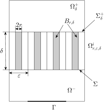
(a) The domain with the thin layer

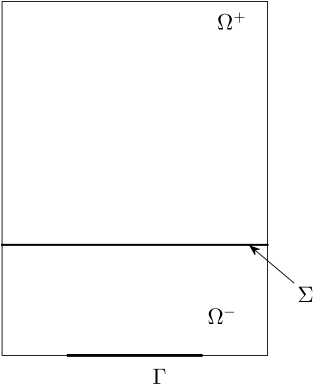
(b) The limit problem

Figure 1: The reference configuration

The structure is fixed on a part $\Gamma$ with non null measure of the boundary $\partial\Omega^{-}\setminus\Sigma$.

We make the following assumptions:

$$r<\frac{\varepsilon}{2},\qquad\frac{r}{\delta}\leq C.$$ (2.6)

Here, the first assumption (2.6)₁ is a non penetration condition for the beams while with the second one, we want to eliminate the case $\displaystyle\frac{\delta}{r}\to 0$ which needs the use of tools for plates (see [1]).

2.2 Strong formulation

Choose an isotropic material with Lamé constants $\lambda^{m},\mu^{m}$ for the beams and another isotropic material with Lamé constants $\lambda^{b},\mu^{b}$ for $\Omega^{-}$ and $\Omega^{+}_{\delta}$. Then we have the following values for the Poisson’s coefficient of the material and Young’s modulus:

$$\nu^{m}=\frac{\lambda^{m}}{2(\lambda^{m}+\mu^{m})},\quad\nu^{b}=\frac{\lambda^{b}}{2(\lambda^{b}+\mu^{b})},$$

$$E^{m}=\frac{\mu^{m}(3\lambda^{m}+2\mu^{m})}{\lambda^{m}+\mu^{m}},\quad E^{b}=\frac{\mu^{b}(3\lambda^{b}+2\mu^{b})}{\lambda^{b}+\mu^{b}}.$$

The symmetric deformation field is defined by

$$(\nabla u)_{S}=\frac{\nabla u+\nabla^{T}u}{2}.$$

The Cauchy stress tensor in $\Omega_{r,\varepsilon,\delta}$ is linked to $(\nabla u_{r,\varepsilon,\delta})_{S}$ through the standard Hooke’s law:

$$\sigma_{r,\varepsilon,\delta}=\left\{\begin{array}[]{ll}\lambda^{b}(\mathrm{Tr}\,(\nabla u_{r,\varepsilon,\delta})_{S})I+2\mu^{b}(\nabla u_{r,\varepsilon,\delta})_{S}&\quad\text{ in }\Omega^{-}\cup\Omega_{\delta}^{+},\\ \lambda^{m}(\mathrm{Tr}\,(\nabla u_{r,\varepsilon,\delta})_{S})I+2\mu^{m}(\nabla u_{r,\varepsilon,\delta})_{S}&\quad\text{ in }\Omega_{r,\varepsilon,\delta}^{i}.\end{array}\right.$$

We consider the standard linear equations of elasticity in $\Omega_{r,\varepsilon,\delta}$. The unknown displacement $u_{r,\varepsilon,\delta}:\Omega_{r,\varepsilon,\delta}\rightarrow{\mathbb{R}}^{3}$ satisfies the following problem:

$$\left\{\begin{array}[]{ll}\nabla\cdot\sigma_{r,\varepsilon,\delta}=-f_{r,\varepsilon,\delta}&\text{in }\Omega_{r,\varepsilon,\delta},\\ u_{r,\varepsilon,\delta}=0&\text{on }\Gamma,\\ \sigma_{r,\varepsilon,\delta}\cdot\nu=0&\text{on }\partial\Omega_{r,\varepsilon,\delta}\setminus\Gamma.\end{array}\right.$$ (2.7)

2.3 Weak formulation

If ${\mathbb{V}}_{r,\varepsilon,\delta}$ denotes the space

$${\mathbb{V}}_{r,\varepsilon,\delta}=\left\{v\in H^{1}(\Omega_{r,\varepsilon,\delta},{\mathbb{R}}^{3})\;|\;v=0\text{ on }\Gamma\right\},$$

the variational formulation of (2.7) is

$$\left\{\begin{array}[]{l}\text{Find }u_{r,\varepsilon,\delta}\in{\mathbb{V}}_{r,\varepsilon,\delta},\\[8.53581pt] \displaystyle\int_{\Omega_{r,\varepsilon,\delta}}\sigma_{r,\varepsilon,\delta}:(\nabla\varphi)_{S}dx=\int_{\Omega_{r,\varepsilon,\delta}}f_{r,\varepsilon,\delta}\cdot\varphi dx,\quad\forall\varphi\in{\mathbb{V}}_{r,\varepsilon,\delta}.\end{array}\right.$$ (2.8)

Throughout the paper and for any $v\in{\mathbb{V}}_{r,\varepsilon,\delta}$ we denote by

$$\sigma(v)=\lambda(\mathrm{Tr}\,(\nabla v)_{S})I+2\mu(\nabla v)_{S}=\left\{\begin{array}[]{ll}\lambda^{b}(\mathrm{Tr}\,(\nabla v)_{S})I+2\mu^{b}(\nabla v)_{S}&\quad\text{ in }\Omega^{-}\cup\Omega_{\delta}^{+},\\[5.69054pt] \lambda^{m}(\mathrm{Tr}\,(\nabla v)_{S})I+2\mu^{m}(\nabla v)_{S}&\quad\text{ in }\Omega_{r,\varepsilon,\delta}^{i}.\end{array}\right.$$

and

$${\cal E}(v)=\int_{\Omega_{r,\varepsilon,\delta}}\sigma(v):(\nabla v)_{S}\,dx$$

the total elastic energy of the displacement $v$. Indeed choosing $v=u_{r,\varepsilon,\delta}$ in (2.8) leads to the usual energy relation

$${\cal E}(u_{r,\varepsilon,\delta})=\int_{\Omega_{r,\varepsilon,\delta}}f_{r,\varepsilon,\delta}\cdot u_{r,\varepsilon,\delta}\,dx.$$ (2.9)

We equip the space ${\mathbb{V}}_{r,\varepsilon,\delta}$ with the following norm:

$$\|u\|_{V}=\|(\nabla u)_{S}\|_{L^{2}(\Omega_{r,\varepsilon,\delta})}.$$

It follows from the 3D–Korn inequality for domain $\Omega^{-}$:

$$\|u\|_{H^{1}(\Omega^{-})}\leq C\|(\nabla u)_{S}\|_{L^{2}(\Omega^{-})}.$$ (2.10)

3 Decomposition of the displacements in $\Omega_{r,\varepsilon,\delta}^{i}$

3.1 Displacement of a single beam. Preliminary estimates

To obtain a priori estimates on $u_{r,\varepsilon,\delta}$ and $(\nabla u_{r,\varepsilon,\delta})_{S}$ we will need Korn’s inequalities for this type of domain. However, for a multi-structure like this, it is not convenient to estimate the constant in a Korn’s type inequality, because the order of each component of the displacement field may be very different. To overcome this difficulty, we will use a decomposition for the displacements of beams. A displacement of the beam $B_{r,d}$ is decomposed as the sum of three fields, the first one stands for the displacement of the center line, the second stands for the rotations of the cross sections and the last one is the warping, it takes into account the deformations of the cross sections.

We recall the definition of the elementary displacement from [1].

Definition 3.1.

The elementary displacement $U_{e}$, associated to $u\in L^{1}(B_{r,d},{\mathbb{R}}^{3})$, is given by

$$U_{e}(x_{1},x_{2},x_{3})=\mathcal{U}(x_{3})+\mathcal{R}(x_{3})\wedge(x_{1}e_{1}+x_{2}e_{2}),\quad\hbox{for a.e. }\;x=(x_{1},x_{2},x_{3})\in B_{r,d},$$ (3.1)

where

$$\left\{\begin{aligned} &\mathcal{U}=\frac{1}{\pi r^{2}}\int_{D_{r}}u(x_{1},x_{2},\cdot)\,dx_{1}dx_{2},\\ &\mathcal{R}_{3}=\frac{2}{\pi r^{4}}\int_{D_{r}}\left(x_{1}u_{2}(x_{1},x_{2},\cdot)-x_{2}u_{1}(x_{1},x_{2},\cdot)\right)\,dx_{1}dx_{2},\\ &\mathcal{R}_{\alpha}=\frac{4(-1)^{3-\alpha}}{\pi r^{4}}\int_{D_{r}}x_{3-\alpha}u_{3}(x_{1},x_{2},\cdot)\,dx_{1}dx_{2},\quad\alpha=1,2.\end{aligned}\right.$$ (3.2)

We write

$$\bar{u}=u-U_{e}.$$ (3.3)

The displacement $\bar{u}$ is the warping. Note that

$$\int_{D_{r}}\bar{u}(x_{1},x_{2},\cdot)\,dx_{1}dx_{2}=0,$$ (3.4)

$$\int_{D_{r}}\left(x_{1}\bar{u}_{2}(x_{1},x_{2},\cdot)-x_{2}\bar{u}_{1}(x_{1},x_{2},\cdot)\right)\,dx_{1}dx_{2}=0,$$

$$\int_{D_{r}}x_{1}\bar{u}_{3}(x_{1},x_{2},\cdot)\;dx_{1}dx_{2}=\int_{D_{r}}x_{2}\bar{u}_{3}(x_{1},x_{2},\cdot)\,dx_{1}dx_{2}=0.$$

The following theorem is proved in [1].

Theorem 3.1.

Let $u$ be in $H^{1}(B_{r,d};{\mathbb{R}}^{3})$ and $u=U_{e}+\bar{u}$ the decomposition of $u$ given by (3.1)–(3.3). There exists a constant $C$ independent of $d$ and $r$ such that the following estimates hold:

$$\begin{aligned} &\|\bar{u}\|_{L^{2}(B_{r,d})}\leq Cr\|(\nabla u)_{S}\|_{L^{2}(B_{r,d})},\qquad\|\nabla\bar{u}\|_{L^{2}(B_{r,d})}\leq C\|(\nabla u)_{S}\|_{L^{2}(B_{r,d})},\\ &\left\|\frac{d\mathcal{R}}{dx_{3}}\right\|_{L^{2}(0,d)}\leq\frac{C}{r^{2}}\|(\nabla u)_{S}\|_{L^{2}(B_{r,d})},\\ &\left\|\frac{d\mathcal{U}}{dx_{3}}-\mathcal{R}\wedge e_{3}\right\|_{L^{2}(0,d)}\leq\frac{C}{r}\|(\nabla u)_{S}\|_{L^{2}(B_{r,d})}.\end{aligned}$$ (3.5)

We set

$$Y_{\varepsilon}=\varepsilon Y,\quad V_{\varepsilon}=Y_{\varepsilon}\times(-\varepsilon,0),\quad B^{\prime}_{r,\varepsilon}=D_{r}\times(-\varepsilon,0),\quad V^{\prime}_{r,\varepsilon,\delta}=V_{\varepsilon}\cup D_{r}\times(-\varepsilon,\delta).$$

Lemma 3.1.

Let $u$ be in $H^{1}(V^{\prime}_{r,\varepsilon,\delta},{\mathbb{R}}^{3})$ and $u=U_{e}+\bar{u}$ the decomposition of the restriction of $u$ to the rod $B^{\prime}_{r,\varepsilon}$ given by (3.1)–(3.3). There exists a constant $C$ independent of $\delta$, $\varepsilon$ and $r$ such that the following estimates hold:

$$\begin{aligned} &|\mathcal{R}(0)|^{2}\leq\frac{C}{r^{3}}\|\nabla u\|^{2}_{L^{2}(V_{\varepsilon})},\\ &\|\mathcal{R}\|^{2}_{L^{2}(0,\delta)}\leq C\frac{\delta}{r^{3}}\|\nabla u\|^{2}_{L^{2}(V_{\varepsilon})}+C\frac{\delta^{2}}{r^{4}}\|(\nabla u)_{S}\|^{2}_{L^{2}(B_{r,\delta})},\\ &\left\|\frac{d\mathcal{U}_{\alpha}}{dx_{3}}\right\|_{L^{2}(0,\delta)}^{2}\leq C\frac{\delta}{r^{3}}\|\nabla u\|^{2}_{L^{2}(V_{\varepsilon})}+C\frac{\delta^{2}}{r^{4}}\|(\nabla u)_{S}\|^{2}_{L^{2}(B_{r,\delta})},\\ &\|\mathcal{U}_{3}-\mathcal{U}_{3}(0)\|^{2}_{L^{2}(0,\delta)}\leq C\frac{\delta^{2}}{r^{2}}\|(\nabla u)_{S}\|^{2}_{L^{2}(B_{r,\delta})},\\ &\|\mathcal{U}_{\alpha}-\mathcal{U}_{\alpha}(0)\|^{2}_{L^{2}(0,\delta)}\leq C\frac{\delta^{3}}{r^{3}}\|\nabla u\|^{2}_{L^{2}(V_{\varepsilon})}+C\frac{\delta^{4}}{r^{4}}\|(\nabla u)_{S}\|^{2}_{L^{2}(B_{r,\delta})},\\ &\|u_{\alpha}(\cdot,\cdot,0)-\mathcal{U}_{\alpha}(0)\|^{2}_{L^{2}(Y_{\varepsilon})}\leq C\varepsilon\|\nabla u\|^{2}_{L^{2}(V_{\varepsilon})}+C\frac{\varepsilon^{2}}{r}\|(\nabla u)_{S}\|^{2}_{L^{2}(V_{\varepsilon})},\\ &\|u_{3}(\cdot,\cdot,0)-\mathcal{U}_{3}(0)\|^{2}_{L^{2}(Y_{\varepsilon})}\leq C\varepsilon\|\nabla u_{3}\|^{2}_{L^{2}(V_{\varepsilon})}+C\frac{\varepsilon^{2}}{r}\|(\nabla u)_{S}\|^{2}_{L^{2}(V_{\varepsilon})}.\end{aligned}$$ (3.6)

Proof.

Applying the 2D-Poincaré-Wirtinger’s inequality we obtain the following estimate:

$$\|u-\mathcal{U}\|_{L^{2}(B^{\prime}_{r,\varepsilon})}\leq Cr\|\nabla u\|_{L^{2}(B^{\prime}_{r,\varepsilon})}$$ (3.7)

The constant does not depend on $r$ and $\varepsilon$.

Step 1. Estimate of $\mathcal{R}(0)$.

Recalling the definition of $\mathcal{R}$ from (3.2) and since $\displaystyle\int_{D_{r}}x_{1}dx_{1}dx_{2}=\int_{D_{r}}x_{2}dx_{1}dx_{2}=0$, we can write

$$\forall x_{3}\in[-\varepsilon,0],\qquad\mathcal{R}_{1}(x_{3})=\frac{4}{\pi r^{4}}\int_{D_{r}}x_{2}\big{(}u_{3}(x)-\mathcal{U}_{3}(x_{3})\big{)}dx_{1}dx_{2}.$$

By Cauchy’s inequality

$$\forall x_{3}\in[-\varepsilon,0],\qquad|\mathcal{R}_{1}(x_{3})|^{2} \leq\frac{16}{\pi^{2}r^{8}}\int_{D_{r}}x^{2}dx_{1}dx_{2}\times\int_{D_{r}}(u_{3}(x)-\mathcal{U}_{3}(x_{3}))^{2}dx_{1}dx_{2}$$

$$\leq\frac{C}{r^{4}}\int_{D_{r}}(u_{3}(x)-\mathcal{U}_{3}(x_{3}))^{2}dx_{1}dx_{2}.$$

Integrating with respect to $x_{3}$ gives

$$\int_{-\varepsilon}^{0}|\mathcal{R}_{1}(x_{3})|^{2}dx_{3}\leq\frac{C}{r^{4}}\int_{B_{r,\varepsilon}}(u(x)-\mathcal{U}(x_{3}))^{2}dx.$$

Using (3.7) we can write

$$\|\mathcal{R}_{1}\|_{L^{2}(-\varepsilon,0)}\leq\frac{C}{r}\|\nabla u\|_{L^{2}(B^{\prime}_{r,\varepsilon})}.$$ (3.8)

The derivative of $\mathcal{R}_{1}$ is equal to $\displaystyle\frac{d\mathcal{R}_{1}}{dx_{3}}(x_{3})=\frac{4}{\pi r^{4}}\int_{D_{r}}x_{2}\frac{\partial u_{3}(x)}{\partial x_{3}}dx_{1}dx_{2}$ for a.e. $x_{3}\in(-\varepsilon,0)$. Then proceeding as above we obtain for a.e. $x_{3}\in(-\varepsilon,0)$

$$\left|\frac{d\mathcal{R}_{1}}{dx_{3}}(x_{3})\right|^{2}\leq\frac{C}{r^{4}}\int_{D_{r}}\left|\frac{\partial u_{3}(x)}{\partial x_{3}}\right|^{2}dx_{1}dx_{2}.$$

Hence

$$\left\|\frac{d\mathcal{R}_{1}}{dx_{3}}\right\|_{L^{2}(-\varepsilon,0)}\leq\frac{C}{r^{2}}\left\|\frac{\partial u_{3}}{\partial x_{3}}\right\|_{L^{2}(B^{\prime}_{r,\varepsilon})}\leq\frac{C}{r^{2}}\|\nabla u\|_{L^{2}(B^{\prime}_{r,\varepsilon})}.$$ (3.9)

We recall the following classical estimates for $\phi\in H^{1}(-a,0)$ ($a>0$)

$$|\phi(0)|^{2}\leq\frac{2}{a}\|\phi\|^{2}_{L^{2}(-a,0)}+\frac{a}{2}\|\phi^{\prime}\|^{2}_{L^{2}(-a,0)},$$ (3.10)

$$\|\phi\|^{2}_{L^{2}(-a,0)}\leq{2a}|\phi(0)|^{2}+{a^{2}}\|\phi^{\prime}\|^{2}_{L^{2}(-a,0)}.$$

Due to (3.8)-(3.9), (3.10)₁ with $a=r$ and since $\varepsilon>r$ that gives for $\mathcal{R}_{1}(0)$

$$|\mathcal{R}_{1}(0)|^{2}\leq\frac{C}{r^{3}}\|\nabla u\|^{2}_{L^{2}(B^{\prime}_{r,\varepsilon})}.$$

The estimates for $\mathcal{R}_{2}(0)$, $\mathcal{R}_{3}(0)$ are obtained in the same way. Hence we get (3.6)₁.

Step 2. Estimate of $\|\mathcal{R}\|_{L^{2}(0,\delta)}$.

The Poincaré’s inequality leads to

$$\|\mathcal{R}-\mathcal{R}(0)\|_{L^{2}(0,\delta)}\leq\delta\left\|\frac{d\mathcal{R}}{dx_{3}}\right\|_{L^{2}(0,\delta)}.$$

From (3.5)₃, (3.10)₂ and (3.6)₁ we get

$$\|\mathcal{R}\|^{2}_{L^{2}(0,\delta)}\leq 2\delta|\mathcal{R}(0)|^{2}+\delta^{2}\left\|\frac{d\mathcal{R}}{dx_{3}}\right\|^{2}_{L^{2}(0,\delta)}\leq C\frac{\delta}{r^{3}}\|\nabla u\|^{2}_{L^{2}(B^{\prime}_{r,\varepsilon})}+C\frac{\delta^{2}}{r^{4}}\|(\nabla u)_{S}\|^{2}_{L^{2}(B_{r,\delta})}.$$ (3.11)

Hence (3.6)₂ is proved.

Step 3. Estimate of $\mathcal{U}-\mathcal{U}(0)$.

Applying inequality (3.5)₄ from Theorem 3.1 the following estimates on $\mathcal{U}$ hold:

$$\begin{aligned} \left\|\frac{d\mathcal{U}_{3}}{dx_{3}}\right\|_{L^{2}(0,\delta)}&\leq\frac{C}{r}\|(\nabla u)_{S}\|_{L^{2}(B_{r,\delta})},\\ \left\|\frac{d\mathcal{U}_{\alpha}}{dx_{3}}\right\|_{L^{2}(0,\delta)}&\leq\|\mathcal{R}\|_{L^{2}(0,\delta)}+\frac{C}{r}\|(\nabla u)_{S}\|_{L^{2}(B_{r,\delta})}.\end{aligned}$$ (3.12)

Combining (3.12)₂ with (3.11) gives

$$\left\|\frac{d\mathcal{U}_{\alpha}}{dx_{3}}\right\|_{L^{2}(0,\delta)}^{2}\leq C\frac{\delta}{r^{3}}\|\nabla u\|^{2}_{L^{2}(B^{\prime}_{r,\varepsilon})}+C\frac{\delta^{2}}{r^{4}}\|(\nabla u)_{S}\|^{2}_{L^{2}(B_{r,\delta})}+\frac{C}{r^{2}}\|(\nabla u)_{S}\|^{2}_{L^{2}(B_{r,\delta})}.$$

Taking into account the assumption (2.6)₂, we obtain (3.6)₃. Then by (3.6)₃, (3.12)₁ and the Poincaré’s inequality (3.6)₄, (3.6)₅ follow.

Step 4. We prove the estimates (3.6)₆-(3.6)₇.

By Korn inequality there exists rigid displacement ${\bf r}$

$$\begin{aligned} &{\bf r}(x)={\bf a}+{\bf b}\wedge\left(x+\frac{\varepsilon}{2}e_{3}\right),\\ &{{\bf a}=\frac{1}{\varepsilon^{3}}\int_{V_{\varepsilon}}u(x)\,dx},\\ &{\bf b}=\frac{6}{\varepsilon^{5}}\int_{V_{\varepsilon}}\left(x+\frac{\varepsilon}{2}e_{3}\right)\wedge u(x)\,dx.\end{aligned}$$

such that

$$\begin{aligned} \|u-{\bf r}\|_{L^{2}(V_{\varepsilon})}\leq C\varepsilon\|(\nabla u)_{S}\|_{L^{2}(V_{\varepsilon})},\\ \|\nabla(u-{\bf r})\|_{L^{2}(V_{\varepsilon})}\leq C\|(\nabla u)_{S}\|_{L^{2}(V_{\varepsilon})}.\end{aligned}$$ (3.13)

Besides by Poincaré-Wirtinger inequality we have

$$\|u_{i}-{\bf a}_{i}\|_{L^{2}(V_{\varepsilon})}\leq C\varepsilon\|\nabla u_{i}\|_{L^{2}(V_{\varepsilon})},\qquad i=1,2,3.$$ (3.14)

The Sobolev embedding theorems give ($V=Y\times(-1,0)$)

$$\|\varphi\|_{L^{4}(Y)}\leq C\|\varphi\|_{H^{1/2}(Y)}\leq C\left(\|\varphi\|_{L^{2}(V)}+\|\nabla\varphi\|_{L^{2}(V)}\right),\quad\forall\varphi\in H^{1}(V).$$

By a change of variables we obtain

$$\|\varphi\|_{L^{4}(Y_{\varepsilon})}\leq C\Big{(}\frac{1}{\varepsilon}\|\varphi\|_{L^{2}(V_{\varepsilon})}+\varepsilon\|\nabla\varphi\|_{L^{2}(V_{\varepsilon})}\Big{)},\quad\forall\varphi\in H^{1}(V_{\varepsilon}).$$

Therefore, (3.13) and the above inequality lead to

$$\|u-{\bf r}\|_{L^{4}(Y_{\varepsilon})}\leq C\|(\nabla u)_{S}\|_{L^{2}(V_{\varepsilon})}.$$ (3.15)

From the identity

$$\frac{1}{\pi r^{2}}\int_{D_{r}}(u(x^{\prime},0)-{\bf r}(x^{\prime},0))dx^{\prime}=\mathcal{U}(0)-{\bf a}-{\bf b}\wedge\frac{\varepsilon}{2}e_{3},$$

estimate (3.15) and the Hölder inequality we get

$$\left|\mathcal{U}(0)-{\bf a}-{\bf b}\wedge\frac{\varepsilon}{2}e_{3}\right|\leq\frac{1}{\pi r^{2}}\left(\int_{D_{r}}1^{4/3}dx^{\prime}\right)^{3/4}\left(\int_{D_{r}}|u(x^{\prime},0)-{\bf r}(x^{\prime},0)|^{4}dx^{\prime}\right)^{1/4}\leq\frac{C}{r^{1/2}}\|(\nabla u)_{S}\|_{L^{2}(V_{\varepsilon})}.$$ (3.16)

As a first consequence, we obtain

$$\left|\mathcal{U}_{3}(0)-{\bf a}_{3}\right|\leq\frac{C}{r^{1/2}}\|(\nabla u)_{S}\|_{L^{2}(V_{\varepsilon})}.$$ (3.17)

From the Cauchy-Schwarz inequality and taking into account (3.14), we derive

$$|{\bf b}|\leq\frac{C}{\varepsilon^{5}}\left(\int_{V_{\varepsilon}}\left|x+\frac{\varepsilon}{2}e_{3}\right|^{2}dx\right)^{1/2}\left(\int_{V_{\varepsilon}}|u(x)-{\bf a}|^{2}dx\right)^{1/2}\\ \leq\frac{C}{\varepsilon^{5}}\cdot\varepsilon\cdot\varepsilon^{3/2}\|u-{\bf a}\|_{L^{2}(V_{\varepsilon})}\leq\frac{C}{\varepsilon^{5/2}}\varepsilon\|\nabla u\|_{L^{2}(V_{\varepsilon})}\leq\frac{C}{\varepsilon^{3/2}}\|\nabla u\|_{L^{2}(V_{\varepsilon})}.$$ (3.18)

Using (3.16) and (3.18) we have

$$\left|\mathcal{U}(0)-{\bf a}\right|\leq\left|\mathcal{U}(0)-{\bf a}-{\bf b}\wedge\frac{\varepsilon}{2}e_{3}\right|+\left|{\bf b}\wedge\frac{\varepsilon}{2}e_{3}\right|\leq\frac{C}{r^{1/2}}\|(\nabla u)_{S}\|_{L^{2}(V_{\varepsilon})}+\frac{C}{\varepsilon^{1/2}}\|\nabla u\|_{L^{2}(V_{\varepsilon})}.$$ (3.19)

Estimates (3.10) and (3.14) yield

$$\|u_{i}(\cdot,\cdot,0)-{\bf a}_{i}\|^{2}_{L^{2}(Y_{\varepsilon})}\leq C\varepsilon\|\nabla u_{i}\|^{2}_{L^{2}(V_{\varepsilon})},\qquad i=1,2,3.$$ (3.20)

Combining (3.19), (3.20) gives

$$\|u_{\alpha}(\cdot,\cdot,0)-\mathcal{U}_{\alpha}(0)\|^{2}_{L^{2}(Y_{\varepsilon})} \leq C(\|u_{\alpha}(\cdot,\cdot,0)-{\bf a}_{\alpha}\|^{2}_{L^{2}(Y_{\varepsilon})}+\|\mathcal{U}_{\alpha}(0)-{\bf a}_{\alpha}\|^{2}_{L^{2}(Y_{\varepsilon})})$$

$$\leq C\varepsilon\|\nabla u\|^{2}_{L^{2}(V_{\varepsilon})}+C\frac{\varepsilon^{2}}{r}\|(\nabla u)_{S}\|^{2}_{L^{2}(V_{\varepsilon})}+C\varepsilon\|\nabla u_{\alpha}\|^{2}_{L^{2}(V_{\varepsilon})}$$

$$\leq C\varepsilon\|\nabla u\|^{2}_{L^{2}(V_{\varepsilon})}+C\frac{\varepsilon^{2}}{r}\|(\nabla u)_{S}\|^{2}_{L^{2}(V_{\varepsilon})},$$

and from (3.17) and again (3.20) we obtain

$$\|u_{3}(\cdot,\cdot,0)-\mathcal{U}_{3}(0)\|^{2}_{L^{2}(Y_{\varepsilon})}\leq C\varepsilon\|\nabla u_{3}\|^{2}_{L^{2}(V_{\varepsilon})}+C\frac{\varepsilon^{2}}{r}\|(\nabla u)_{S}\|^{2}_{L^{2}(V_{\varepsilon})},$$

Hence we get (3.6)₆-(3.6)₇. ∎

4 A priori estimates

In this section all the constants do not depend on $\varepsilon,\delta$ and $r$. We denote $x^{\prime}=(x_{1},x_{2})$ the running point of ${\mathbb{R}}^{2}$.

4.1 Decomposition of the displacements in $\Omega_{r,\varepsilon,\delta}^{i}$

We decompose the displacement $u\in{\mathbb{V}}_{r,\varepsilon,\delta}$ in each beam $\varepsilon{\bf i}+B_{r,\delta}$, ${\bf i}\in\widehat{\Xi}_{\varepsilon}\times\{0\}$ as in the Definition 3.1. The components of the elementary displacement are denoted ${\cal U}_{\xi}$, ${\cal R}_{\xi}$, where $\xi=\displaystyle\left[\frac{x^{\prime}}{\varepsilon}\right]_{Y}$.

Now we define the fields $\widetilde{\mathcal{U}}$, $\widetilde{\mathcal{R}}$ and $\widetilde{\bar{u}}$ for a.e. $x\in B_{r,\delta},s\in\omega$ by

$$\widetilde{\mathcal{U}}(s_{1},s_{2},x_{3})=\left\{\begin{aligned} &\mathcal{U}_{\xi}(x_{3}),&\hbox{if}\;\;\xi=\left[\frac{s}{\varepsilon}\right]\in\widehat{\Xi}_{\varepsilon}\\ &0,&\hbox{if}\;\;\xi\not\in\widehat{\Xi}_{\varepsilon}\\ \end{aligned}\right.,\qquad\widetilde{\mathcal{R}}(s_{1},s_{2},x_{3})=\left\{\begin{aligned} &\mathcal{R}_{\xi}(x_{3}),&\hbox{if}\;\;\xi=\left[\frac{s}{\varepsilon}\right]\in\widehat{\Xi}_{\varepsilon}\\ &0,&\hbox{if}\;\;\xi\not\in\widehat{\Xi}_{\varepsilon}\end{aligned}\right.,$$

$$\widetilde{\bar{u}}(s_{1},s_{2},x)=\left\{\begin{aligned} &\bar{u}_{\xi}(x),&\hbox{if}\;\;\xi=\left[\frac{s}{\varepsilon}\right]\in\widehat{\Xi}_{\varepsilon}\\ &0,&\hbox{if}\;\;\xi\not\in\widehat{\Xi}_{\varepsilon}\end{aligned}\right..$$

We have

$$\widetilde{\mathcal{U}},\widetilde{\mathcal{R}}\in L^{2}(\omega,H^{1}((0,\delta),{\mathbb{R}}^{3})),\quad\widetilde{\bar{u}}\in L^{2}(\omega,H^{1}(B_{r,\delta},{\mathbb{R}}^{3})).$$

Moreover,

$$\|\widetilde{\mathcal{U}}\|^{2}_{L^{2}(\omega\times(0,\delta))}=\varepsilon^{2}\sum_{\xi\in\widehat{\Xi}_{\varepsilon}}\|\mathcal{U}_{\xi}\|^{2}_{L^{2}(0,\delta)},\quad\|\widetilde{\mathcal{R}}\|^{2}_{L^{2}(\omega\times(0,\delta))}=\varepsilon^{2}\sum_{\xi\in\widehat{\Xi}_{\varepsilon}}\|\mathcal{R}_{\xi}\|^{2}_{L^{2}(0,\delta)},$$

$$\|\widetilde{\bar{u}}\|^{2}_{L^{2}(\omega\times B_{r,\delta})}=\varepsilon^{2}\sum_{\xi\in\widehat{\Xi}_{\varepsilon}}\|\bar{u}_{\xi}\|^{2}_{L^{2}(B_{r,\delta})}.$$

As a consequence of the Theorem 3.1 and Lemma 3.1 we get

Lemma 4.1.

Let $u$ be in ${\mathbb{V}}_{r,\varepsilon,\delta}$. The following estimates hold:

$$\Big{\|}\frac{\partial\widetilde{\mathcal{R}}}{\partial x_{3}}\Big{\|}_{L^{2}(\omega\times(0,\delta))}\leq C\frac{\varepsilon}{r^{2}}\|u\|_{V},$$ (4.1)

$$\Big{\|}\frac{\partial\widetilde{\mathcal{U}}}{\partial x_{3}}-\widetilde{\mathcal{R}}\land e_{3}\Big{\|}_{L^{2}(\omega\times(0,\delta))}\leq C\frac{\varepsilon}{r}\|u\|_{V},$$

$$\|\nabla_{x}\widetilde{\bar{u}}\|_{L^{2}(\omega\times B_{r,\delta})}\leq C\varepsilon\|u\|_{V},$$

$$\|\widetilde{\bar{u}}\|_{L^{2}(\omega\times B_{r,\delta})}\leq C\varepsilon r\|u\|_{V},$$

$$\|\widetilde{\mathcal{R}}\|_{L^{2}(\omega\times(0,\delta))}\leq C\frac{\varepsilon\delta}{r^{2}}\|u\|_{V},$$

$$\Big{\|}\frac{\partial\widetilde{\mathcal{U}}_{\alpha}}{\partial x_{3}}\Big{\|}_{L^{2}(\omega\times(0,\delta))}\leq C\frac{\varepsilon\delta}{r^{2}}\|u\|_{V}.$$

Moreover,

$$\|\widetilde{\mathcal{R}}(\cdot,\cdot,0)\|^{2}_{L^{2}(\widehat{\omega}_{\varepsilon})}\leq C\frac{\varepsilon^{2}}{r^{3}}\|u\|^{2}_{V},$$ (4.2)

$$\|\widetilde{\mathcal{R}}(\cdot,\cdot,\delta)\|^{2}_{L^{2}(\widehat{\omega}_{\varepsilon})}\leq C\frac{\varepsilon^{2}}{r^{3}}\|\nabla u\|^{2}_{L^{2}(\Omega^{+}_{\delta})},$$

$$\|\widetilde{\mathcal{U}}_{3}-\widetilde{\mathcal{U}}_{3}(\cdot,\cdot,0)\|_{L^{2}(\omega\times(0,\delta))}\leq C\frac{\delta\varepsilon}{r}\|u\|_{V},$$

$$\|\widetilde{\mathcal{U}}_{\alpha}-\widetilde{\mathcal{U}}_{\alpha}(\cdot,\cdot,0)\|_{L^{2}(\omega\times(0,\delta))}\leq C\frac{\delta^{2}\varepsilon}{r^{2}}\|u\|_{V},\quad\text{where }\alpha=1,2.$$

Proof.

Estimates (4.1)₁ – (4.1)₆ follow directly from (2.10), (3.5)₃, (3.5)₄ and (3.6)₂–(3.6)₃ and estimates (4.2)₁ – (4.2)₄ are the consequences of the estimates in Lemma 3.1 and (2.10). ∎

4.2 Estimates of the interface traces

Lemma 4.2.

There exists a constant $C$ independent of $\varepsilon,\delta,r$ such that for any $u\in{\mathbb{V}}_{r,\varepsilon,\delta}$

$$\|u(\cdot,\cdot,0)-\widetilde{\mathcal{U}}(\cdot,\cdot,0)\|^{2}_{L^{2}(\widehat{\omega}_{\varepsilon})}\leq C\frac{\varepsilon^{2}}{r}\|u\|^{2}_{V},$$ (4.3)

$$\|u_{\alpha}(\cdot,\cdot,\delta)-\widetilde{\mathcal{U}}_{\alpha}(\cdot,\cdot,\delta)\|^{2}_{L^{2}(\widehat{\omega}_{\varepsilon})}\leq C\varepsilon\|\nabla u_{\alpha}\|^{2}_{L^{2}(\Omega^{+}_{\delta})}+C\frac{\varepsilon^{2}}{r}\|u\|^{2}_{V},$$ (4.4)

$$\|u_{3}(\cdot,\cdot,\delta)-\widetilde{\mathcal{U}}_{3}(\cdot,\cdot,\delta)\|^{2}_{L^{2}(\widehat{\omega}_{\varepsilon})}\leq C\varepsilon\|\nabla u_{3}\|^{2}_{L^{2}(\Omega^{+}_{\delta})}+C\frac{\varepsilon^{2}}{r}\|u\|^{2}_{V}.$$

Moreover,

$$\|u_{\alpha}(\cdot,\cdot,\delta)-u_{\alpha}(\cdot,\cdot,0)\|^{2}_{L^{2}(\widehat{\omega}_{\varepsilon})}\leq C\varepsilon\|\nabla u_{\alpha}\|^{2}_{L^{2}(\Omega^{+}_{\delta})}+C\frac{\varepsilon^{2}\delta^{3}}{r^{4}}\|u\|^{2}_{V},$$ (4.5)

$$\|u_{3}(\cdot,\cdot,\delta)-u_{3}(\cdot,\cdot,0)\|^{2}_{L^{2}(\widehat{\omega}_{\varepsilon})}\leq C\varepsilon\|\nabla u_{3}\|^{2}_{L^{2}(\Omega^{+}_{\delta})}+C\frac{\varepsilon^{2}\delta}{r^{2}}\|u\|^{2}_{V}.$$ (4.6)

Proof.

Using (3.6)₆-(3.6)₇ and then summing over all cells give (4.3). In the same way the estimates (4.4) are derived.

Applying (4.1)₂ we write

$$\|\widetilde{\mathcal{U}}_{3}(\cdot,\cdot,\delta)-\widetilde{\mathcal{U}}_{3}(\cdot,\cdot,0)\|_{L^{2}(\widehat{\omega}_{\varepsilon})}^{2}\leq\delta\left\|\frac{\partial\widetilde{\mathcal{U}}_{3}}{\partial x_{3}}\right\|^{2}_{L^{2}(\widehat{\omega}_{\varepsilon}\times(0,\delta))}\leq C\frac{\varepsilon^{2}\delta}{r^{2}}\|u\|^{2}_{V}.$$ (4.7)

From (4.1)₆ we have

$$\|\widetilde{\mathcal{U}}_{\alpha}(\cdot,\cdot,\delta)-\widetilde{\mathcal{U}}_{\alpha}(\cdot,\cdot,0)\|_{L^{2}(\widehat{\omega}_{\varepsilon})}^{2}\leq C\frac{\varepsilon^{2}\delta^{3}}{r^{4}}\|u\|^{2}_{V}.$$ (4.8)

Using (4.8) and the above estimates we obtain (4.5), (4.6). ∎

4.3 Estimates of the displacements in $\Omega_{\delta}^{+}$

Lemma 4.3.

There exists a constant $C$ which does not depend on $\varepsilon$, $r$ and $\delta$, such that for any $u\in{\mathbb{V}}_{r,\varepsilon,\delta}$

$$\|u_{\alpha}\|_{H^{1}(\Omega_{\delta}^{+})}\leq C\Big{(}\frac{\varepsilon\delta^{3/2}}{r^{2}}+1\Big{)}\|u\|_{V},$$ (4.9)

$$\|u_{3}\|_{H^{1}(\Omega_{\delta}^{+})}\leq C\Big{(}\frac{\varepsilon\delta^{1/2}}{r}+1\Big{)}\|u\|_{V},$$ (4.10)

where $\alpha=1,2$.

Proof.

From the Korn’s inequality and the trace theorem we derive

$$\begin{aligned} &\|u\|_{L^{2}(\Sigma)}&\leq\quad&C\|u\|_{H^{1}(\Omega^{-})}\leq C\|(\nabla u)_{S}\|_{L^{2}(\Omega^{-})},\\ &\|u\|_{H^{1}(\Omega_{\delta}^{+})}&\leq\quad&C\big{(}\|(\nabla u)_{S}\|_{L^{2}(\Omega_{\delta}^{+})}+\|u\|_{L^{2}(\Sigma^{+}_{\delta})}\big{)}.\end{aligned}$$ (4.11)

We know that there exists a rigid displacement ${\bf r}$

$$\forall x\in{\mathbb{R}}^{3},\qquad{\bf r}(x)={\bf a}+{\bf b}\land(x-\delta e_{3}),\qquad{\bf a},\;{\bf b}\in{\mathbb{R}}^{3},$$

such that

$$\|u-{\bf r}\|_{L^{2}(\Sigma_{\delta}^{+})}\leq C\|u-{\bf r}\|_{H^{1}(\Omega_{\delta}^{+})}\leq C\|(\nabla u)_{S}\|_{L^{2}(\Omega_{\delta}^{+})}.$$ (4.12)

The constant does not depend on $\delta$. Then, we get

$$\|(u-{\bf r})(\cdot,\cdot,\delta)\|_{L^{2}(\widehat{\omega}_{\varepsilon})}\leq\|u-{\bf r}\|_{L^{2}(\Sigma_{\delta}^{+})}\leq C\|(\nabla u)_{S}\|_{L^{2}(\Omega_{\delta}^{+})}.$$ (4.13)

Using

$$\|u(\cdot,\cdot,0)\|_{L^{2}(\widehat{\omega}_{\varepsilon})}\leq\|u\|_{L^{2}(\Sigma)}\leq C\|(\nabla u)_{S}\|_{L^{2}(\Omega^{-})}\leq C\|u\|_{V},$$ (4.14)

from (4.5), (4.6) we obtain

$$\begin{aligned} \|u_{\alpha}(\cdot,\cdot,\delta)\|_{L^{2}(\widehat{\omega}_{\varepsilon})}\leq C\varepsilon^{1/2}\|\nabla u_{\alpha}\|_{L^{2}(\Omega^{+}_{\delta})}+C\frac{\varepsilon\delta^{3/2}}{r^{2}}\|u\|_{V}+C\|u\|_{V},\\ \|u_{3}(\cdot,\cdot,\delta)\|_{L^{2}(\widehat{\omega}_{\varepsilon})}\leq C\varepsilon^{1/2}\|\nabla u_{3}\|_{L^{2}(\Omega^{+}_{\delta})}+C\frac{\varepsilon\delta^{1/2}}{r}\|u\|_{V}+C\|u\|_{V}.\end{aligned}$$ (4.15)

Combining this with (4.13) gives

$$\begin{aligned} \|{\bf r}_{\alpha}(\cdot,\cdot,\delta)\|_{L^{2}(\widehat{\omega}_{\varepsilon})}\leq C\varepsilon^{1/2}\|\nabla u_{\alpha}\|_{L^{2}(\Omega^{+}_{\delta})}+C\frac{\varepsilon\delta^{3/2}}{r^{2}}\|u\|_{V}+C\|u\|_{V},\\ \|{\bf r}_{3}(\cdot,\cdot,\delta)\|_{L^{2}(\widehat{\omega}_{\varepsilon})}\leq C\varepsilon^{1/2}\|\nabla u_{3}\|_{L^{2}(\Omega^{+}_{\delta})}+C\frac{\varepsilon\delta^{1/2}}{r}\|u\|_{V}+C\|u\|_{V}.\end{aligned}$$ (4.16)

Therefore,

$$|{\bf a_{1}}|+|{\bf a_{2}}|+|{\bf b_{3}}|\leq C\varepsilon^{1/2}\|\nabla u_{\alpha}\|_{L^{2}(\Omega^{+}_{\delta})}+C\frac{\varepsilon\delta^{3/2}}{r^{2}}\|u\|_{V}+C\|u\|_{V},$$

$$|{\bf a_{3}}|+|{\bf b_{1}}|+|{\bf b_{2}}|\leq C\varepsilon^{1/2}\|\nabla u_{3}\|_{L^{2}(\Omega^{+}_{\delta})}+C\frac{\varepsilon\delta^{1/2}}{r}\|u\|_{V}+C\|u\|_{V}.$$

These estimates together with (4.12) allow to obtain estimates on $u_{1},u_{2},u_{3}$. From this we have

$$\begin{aligned} \|u_{\alpha}\|_{H^{1}(\Omega_{\delta}^{+})}\leq C\varepsilon^{1/2}\|\nabla u_{\alpha}\|_{L^{2}(\Omega^{+}_{\delta})}+C\frac{\varepsilon\delta^{3/2}}{r^{2}}\|u\|_{V}+C\|u\|_{V},\\ \|u_{3}\|_{H^{1}(\Omega_{\delta}^{+})}\leq C\varepsilon^{1/2}\|\nabla u_{3}\|_{L^{2}(\Omega^{+}_{\delta})}+C\frac{\varepsilon\delta^{1/2}}{r}\|u\|_{V}+C\|u\|_{V}.\end{aligned}$$ (4.17)

Therefore, for $\varepsilon$ small enough the following hold true:

$$\|\nabla u_{\alpha}\|_{L^{2}(\Omega_{\delta}^{+})}\leq C\frac{\varepsilon\delta^{3/2}}{r^{2}}\|u\|_{V}+C\|u\|_{V},\qquad\|\nabla u_{3}\|_{L^{2}(\Omega_{\delta}^{+})}\leq C\frac{\varepsilon\delta^{1/2}}{r}\|u\|_{V}+C\|u\|_{V}.$$

Inserting that in (4.17) we derive (4.9)-(4.10). ∎

As a consequence of Lemma 4.3, the estimates (4.5), (4.6) can be replaced by

$$\|u_{\alpha}(\cdot,\cdot,\delta)-u_{\alpha}(\cdot,\cdot,0)\|^{2}_{L^{2}(\widehat{\omega}_{\varepsilon})}\leq C\frac{\varepsilon^{2}\delta^{3}}{r^{4}}\|u\|^{2}_{V},$$ (4.18)

$$\|u_{3}(\cdot,\cdot,\delta)-u_{3}(\cdot,\cdot,0)\|^{2}_{L^{2}(\widehat{\omega}_{\varepsilon})}\leq C\frac{\varepsilon^{2}\delta}{r^{2}}\|u\|^{2}_{V}.$$ (4.19)

4.4 Estimates for the set of beams $\Omega_{r,\varepsilon,\delta}^{i}$

Lemma 4.4.

There exists a constant $C$ which does not depend on $\varepsilon$, $r$ and $\delta$, such that for any $u\in{\mathbb{V}}_{r,\varepsilon,\delta}$

$$\|\nabla u\|_{L^{2}(\Omega_{r,\varepsilon,\delta}^{i})} \leq C\frac{\delta}{r}\|u\|_{V},$$ (4.20)

$$\|u_{3}\|_{L^{2}(\Omega_{r,\varepsilon,\delta}^{i})} \leq C\frac{r\delta^{1/2}}{\varepsilon}\|u\|_{V},$$

$$\|u_{\alpha}\|_{L^{2}(\Omega_{r,\varepsilon,\delta}^{i})} \leq C\frac{r\delta^{1/2}}{\varepsilon}\left(1+\frac{\varepsilon\delta^{3/2}}{r^{2}}\right)\|u\|_{V}$$

where $\alpha=1,2$.

Proof.

From the estimates in Theorem 3.1, (3.6)₂ and (3.6)₃ and after summation over all the beams, we get (we make use of the assumption (2.6)₂)

$$\|\nabla u\|^{2}_{L^{2}(\Omega_{r,\varepsilon,\delta}^{i})}\leq C\left(\frac{\delta}{r}\|\nabla u\|^{2}_{L^{2}(\Omega^{-})}+\frac{\delta^{2}}{r^{2}}\|(\nabla u)_{S}\|^{2}_{L^{2}(\Omega_{r,\varepsilon,\delta}^{i})}\right)\leq C\frac{\delta^{2}}{r^{2}}\|u\|^{2}_{V}.$$ (4.21)

From (4.3) and (4.11)₁, it follows that

$$\sum_{\xi\in\Xi_{\varepsilon}}\varepsilon^{2}|\mathcal{U}_{\xi}(0)|^{2}=\|\widetilde{\mathcal{U}}(\cdot,\cdot,0)\|^{2}_{L^{2}(\widehat{\omega}_{\varepsilon})}\leq C\frac{\varepsilon^{2}}{r}\|u\|^{2}_{V}+C\|u\|^{2}_{V},$$

$$\sum_{\xi\in\Xi_{\varepsilon}}|\mathcal{U}_{\xi}(0)|^{2}\leq C\left(\frac{1}{r}+\frac{1}{\varepsilon^{2}}\right)\|u\|^{2}_{V}.$$

Using (3.5)₄, (3.6)₃, (3.10), we obtain

$$\begin{aligned} \sum_{\xi\in\Xi_{\varepsilon}}\|\mathcal{U}_{\xi,3}\|^{2}_{L^{2}(0,\delta)}\leq C\left(\frac{\delta}{\varepsilon^{2}}+\frac{\delta^{2}}{r^{2}}\right)\|u\|^{2}_{V},\\ \sum_{\xi\in\Xi_{\varepsilon}}\|\mathcal{U}_{\xi,\alpha}\|^{2}_{L^{2}(0,\delta)}\leq C\left(\frac{\delta}{\varepsilon^{2}}+\frac{\delta^{4}}{r^{4}}\right)\|u\|^{2}_{V}.\end{aligned}$$ (4.22)

Additionally,

$$\sum_{\xi\in\Xi_{\varepsilon}}\|\bar{u}_{\xi}\|^{2}_{L^{2}(B_{r,\delta})}\leq Cr^{2}\|(\nabla u)_{S}\|^{2}_{L^{2}(\Omega_{r,\varepsilon,\delta}^{i})}\leq Cr^{2}\|u\|^{2}_{V}.$$ (4.23)

Then (3.6)₂, (4.22) and (4.23) give

$$\sum_{\xi\in\Xi_{\varepsilon}}\|u_{\xi,\alpha}\|^{2}_{L^{2}(B_{r,\delta})}\leq C\left(\frac{r^{2}\delta}{\varepsilon^{2}}+\frac{\delta^{4}}{r^{2}}+\delta^{2}+r^{2}\right)\|u\|^{2}_{V}\leq C\frac{r^{2}\delta}{\varepsilon^{2}}\left(1+\frac{\varepsilon^{2}\delta^{3}}{r^{4}}\right)\|u\|^{2}_{V},$$

$$\sum_{\xi\in\Xi_{\varepsilon}}\|u_{\xi,3}\|^{2}_{L^{2}(B_{r,\delta})}\leq C\left(\frac{r^{2}\delta}{\varepsilon^{2}}+\delta^{2}+r^{2}\right)\|u\|^{2}_{V}\leq C\frac{r^{2}\delta}{\varepsilon^{2}}\left(1+\frac{\varepsilon^{2}\delta}{r^{2}}\right)\|u\|^{2}_{V}.$$

From the last inequalities we derive (4.20)₂ and (4.20)₃. ∎

4.5 The limit cases

In view of the conditions (2.6) and the estimates in Lemma 4.3, and in order that the lower and upper parts of our structure match, we must assume that

$$\frac{\varepsilon^{2}\delta^{3}}{r^{4}}\hbox{ is uniformly bounded from above}.$$ (4.24)

From now on, the parameters $r$, $\delta$ and $\varepsilon$ are linked in this way

• $r=\kappa_{0}\varepsilon^{\eta_{0}}$, $\eta_{0}\geq 1$, $\kappa_{0}>0$, if $\eta_{0}=1$ then $\kappa_{0}\in(0,1/2)$ (non penetration condition),

• $\delta=\kappa_{1}\varepsilon^{\eta_{1}}$, $\kappa_{1}>0$ and $\eta_{1}\leq\eta_{0}$.

The above assumption (4.24) yields

$$2+3\eta_{1}-4\eta_{0}\geq 0.$$

Hence, the couple $(\eta_{0},\eta_{1})$ belongs to the triangle whose vertexes are

$$(2/3,1),\qquad(1,1),\qquad(2,2).$$ (4.25)

The case

$$\lim_{\varepsilon\to 0}{\varepsilon^{2}\delta^{3}\over r^{4}}=0$$

could be very easily analysed. Using the estimates (4.18)-(4.19), in this case we can prove that, the limit displacements on both parts coincide on the interface; hence the limit displacement belongs to $H^{1}(\omega\times(-L,L),{\mathbb{R}}^{3})$ and it is the solution of an elasticity system.

Therefore, the most interesting cases correspond to $\displaystyle\lim_{\varepsilon\to 0}{\varepsilon^{2}\delta^{3}\over r^{4}}>0$; this is the critical situation

• (i) $r=\kappa_{0}\varepsilon$, $\kappa_{0}\in(0,1/2)$ and $\delta=\kappa_{1}\varepsilon^{2/3}$, $\kappa_{1}>0$,

• (ii) $r=\kappa_{0}\varepsilon^{\eta_{0}}$, $\eta_{0}\in(1,2)$, $\kappa_{0}>0$ and $\delta=\kappa_{1}\varepsilon^{(4\eta_{0}-2)/3}$, $\kappa_{1}>0$.

We obtain the edge of the triangle with the vertexes $(2/3,1)$ and $(2,2)$. We eliminate the case $\eta_{0}=\eta_{1}=2$ to deal with small beams in the layer.

For the sake of simplicity, from now on we will use the following notations:

• $\Omega_{\varepsilon}$ instead of $\Omega_{r,\varepsilon,\delta}$,

• $\Omega_{\varepsilon}^{i}$ instead of $\Omega_{r,\varepsilon,\delta}^{i}$,

• $\Omega_{\varepsilon}^{+}$ instead of $\Omega_{\delta}^{+}$,

• $\sigma_{\varepsilon}$ instead of $\sigma_{r,\varepsilon,\delta}$,

• $u_{\varepsilon}$ instead of $u_{r,\varepsilon,\delta}$,

• $f_{\varepsilon}$ instead of $f_{r,\varepsilon,\delta}$.

With assumption (4.24) we can rewrite some estimates obtained above. For any $u\in{\mathbb{V}}_{r,\varepsilon,\delta}$ we have

$$\|u\|_{L^{2}(\Omega_{\varepsilon}^{i})}\leq C\frac{r\delta^{1/2}}{\varepsilon}\|u\|_{V},$$ (4.26)

$$\|u\|_{H^{1}(\Omega_{\varepsilon}^{+})}\leq C\|u\|_{V}.$$ (4.27)

The constants do not depend on $\varepsilon$, $r$ and $\delta$.

4.6 Force assumptions

We set

$$B_{1}=D_{1}\times(0,1).$$

To obtain estimates on $u_{\varepsilon}$ we test (2.8) with $\varphi=u_{\varepsilon}$. We have

$$M_{1}\|u_{\varepsilon}\|^{2}_{V}\leq\|f_{\varepsilon}\|_{L^{2}(\Omega_{\varepsilon},{\mathbb{R}}^{3})}\|u_{\varepsilon}\|_{L^{2}(\Omega_{\varepsilon},{\mathbb{R}}^{3})}.$$ (4.28)

We consider the following assumption on the applied forces:

$$f_{\varepsilon}(x)=\left\{\begin{aligned} &\displaystyle\frac{\varepsilon^{2}}{r^{2}\delta}\,F^{m}\left(\varepsilon\left[\frac{x^{\prime}}{\varepsilon}\right]_{Y},\frac{\varepsilon}{r}\left\{\frac{x^{\prime}}{\varepsilon}\right\}_{Y},\frac{x_{3}}{\delta}\right)\enskip\hbox{for a.e.}\;\;x\in\Omega_{\varepsilon}^{i},\\[5.69054pt] &F(x)\hskip 110.96574pt\hbox{for a.e.}\;\;x\in\Omega^{-}\cup\Omega^{+}_{\varepsilon},\end{aligned}\right.$$ (4.29)

where $F^{m}\in{\cal C}^{0}(\overline{\omega},L^{2}(B_{1},{\mathbb{R}}^{3}))$, $F\in L^{2}(\omega\times(-L,L),{\mathbb{R}}^{3})$. Then,

$$\|f_{\varepsilon}\|_{L^{2}(\Omega^{i}_{\varepsilon},{\mathbb{R}}^{3})}\leq\frac{\varepsilon}{r\delta^{1/2}}\|F^{m}\|_{L^{\infty}(\omega,L^{2}(B_{1},{\mathbb{R}}^{3}))}.$$

Making use of the estimates (2.10), (4.26), (4.27) together with inequality (4.28) yield

$$\|u_{\varepsilon}\|_{V}\leq C$$ (4.30)

The constant does not depend of $r$, $\varepsilon$ and $\delta$.

As mention above, from now on, we only consider the cases (i) and (ii) introduced in Section 4.5.

5 The periodic unfolding operators

Definition 5.1.

For $\varphi$ Lebesgue-measurable function on $\omega\times(0,\delta)$, the unfolding operator $\mathcal{T}_{\varepsilon}$ is defined as follows:

$$\mathcal{T}_{\varepsilon}(\varphi)(s_{1},s_{2},X_{3})=\left\{\begin{array}[]{ll}\varphi(s_{1},s_{2},\delta X_{3}),&\text{ for a.e. }\;\;(s_{1},s_{2},X_{3})\in\widehat{\omega}_{\varepsilon}\times(0,1),\\ 0,&\text{ for a.e. }\;\;(s_{1},s_{2},X_{3})\in\Lambda_{\varepsilon}\times(0,1).\end{array}\right.$$

Definition 5.2.

For $\varphi$ Lebesgue-measurable function on $\omega\times B_{r,\delta}$, the unfolding operator $\mathcal{T}^{\prime}_{\varepsilon}$ is defined as follows:

$$\mathcal{T}^{{}^{\prime}}_{\varepsilon}(\varphi)(s_{1},s_{2},X_{1},X_{2},X_{3})=\left\{\begin{array}[]{ll}\varphi(s_{1},s_{2},rX_{1},rX_{2},\delta X_{3}),&\text{ for a.e. }\;\;(s_{1},s_{2},X_{1},X_{2},X_{3})\in\widehat{\omega}_{\varepsilon}\times B_{1},\\ 0,&\text{ for a.e. }\;\;(s_{1},s_{2},X_{1},X_{2},X_{3})\in\Lambda_{\varepsilon}\times B_{1}.\end{array}\right.$$

Observe that if $\varphi$ is a Lebesgue-measurable function on $\omega\times(0,\delta)$ then $\mathcal{T}_{\varepsilon}(\varphi)=\mathcal{T}_{\varepsilon}^{{}^{\prime}}(\varphi)$.

Lemma 5.1.

(Properties of the operators $\mathcal{T}_{\varepsilon}$, $\mathcal{T}_{\varepsilon}^{{}^{\prime}}$)

1. $\forall v,w\in L^{2}(\omega\times(0,\delta))$

   $$\mathcal{T}_{\varepsilon}(vw)=\mathcal{T}_{\varepsilon}(v)\mathcal{T}_{\varepsilon}(w),$$

   
   

   $\forall v,w\in L^{2}(\omega\times B_{r,\delta})$

   $$\mathcal{T}_{\varepsilon}^{{}^{\prime}}(vw)=\mathcal{T}_{\varepsilon}^{{}^{\prime}}(v)\mathcal{T}_{\varepsilon}^{{}^{\prime}}(w).$$

2. $\forall u\in L^{1}(\omega\times(0,\delta))$

   $$\delta\int_{\omega\times(0,1)}\mathcal{T}_{\varepsilon}(u)\,ds_{1}\,ds_{2}\,dX_{3}=\int_{\widehat{\omega}_{\varepsilon}\times(0,\delta)}u\,ds_{1}\,ds_{2}\,dx_{3},$$

   $\forall u\in L^{1}(\omega\times B_{r,\delta})$

   $$r^{2}\delta\int_{\omega\times B_{1}}\mathcal{T}_{\varepsilon}^{{}^{\prime}}(u)\,ds_{1}\,ds_{2}\,dX_{1}\,dX_{2}\,dX_{3}=\int_{\widehat{\omega}_{\varepsilon}\times B_{r,\delta}}u\,ds_{1}\,ds_{2}\,dx_{1}\,dx_{2}\,dx_{3}.$$

3. $\forall u\in L^{2}(\omega\times(0,\delta))$

   $$\|\mathcal{T}_{\varepsilon}(u)\|_{L^{2}(\omega\times(0,1))}\leq\frac{1}{\sqrt{\delta}}\|u\|_{L^{2}(\omega\times(0,\delta))},$$

   $\forall u\in L^{2}(\omega\times B_{r,\delta})$

   $$\|\mathcal{T}_{\varepsilon}^{{}^{\prime}}(u)\|_{L^{2}(\omega\times B_{1})}\leq\frac{1}{r\sqrt{\delta}}\|u\|_{L^{2}(\omega\times B_{r,\delta})}.$$

4. Let $u$ be in $L^{2}(\omega,H^{1}(0,\delta))$, a.e. in $\omega\times(0,1)$ we have

   $$\delta\mathcal{T}_{\varepsilon}(\nabla_{x_{3}}u)=\nabla_{X_{3}}\mathcal{T}_{\varepsilon}(u).$$

   Let $u$ be in $L^{2}(\omega,H^{1}(B_{r,\delta}))$., a.e. in $\omega\times B_{1}$ we have

   $$r\mathcal{T}_{\varepsilon}^{{}^{\prime}}(\nabla_{x_{\alpha}}u)=\nabla_{X_{\alpha}}\mathcal{T}_{\varepsilon}^{{}^{\prime}}(u),\quad\delta\mathcal{T}_{\varepsilon}^{{}^{\prime}}(\nabla_{x_{3}}u)=\nabla_{X_{3}}\mathcal{T}_{\varepsilon}^{{}^{\prime}}(u),\text{ where }\alpha=1,2.$$

Proof.

Properties 1-3 are obtained similarly as in the proof of Lemma 5.1 of [3].

Property 4 is the direct consequence chain rule formulae:

$$\frac{\partial(\mathcal{T}_{\varepsilon}^{{}^{\prime}}(u))}{\partial X_{\alpha}}=r\mathcal{T}_{\varepsilon}^{{}^{\prime}}\left(\frac{\partial u}{\partial x_{\alpha}}\right),\quad\alpha=1,2,$$

$$\frac{\partial(\mathcal{T}_{\varepsilon}(u))}{\partial X_{3}}=\delta\mathcal{T}_{\varepsilon}\left(\frac{\partial u}{\partial x_{3}}\right),\quad\frac{\partial(\mathcal{T}_{\varepsilon}^{{}^{\prime}}(u))}{\partial X_{3}}=\delta\mathcal{T}_{\varepsilon}^{{}^{\prime}}\left(\frac{\partial u}{\partial x_{3}}\right).$$

∎

5.1 The limit fields (Cases (i) and (ii))

From now on, $(u_{\varepsilon})_{\alpha}$ will be denoted as $u_{\varepsilon,\alpha}$; the same notation will be used for the fields with values in ${\mathbb{R}}^{2}$ or ${\mathbb{R}}^{3}$.

From Lemmas 4.1 and 5.1 we obtain the following result.

Lemma 5.2.

There exists a constant $C$ independent of $\varepsilon$, $\delta$ and $r$ such that

$$\|\mathcal{T}_{\varepsilon}(\widetilde{\mathcal{U}}_{\varepsilon})\|_{L^{2}(\omega,H^{1}(0,1))}\leq C,$$ (5.1)

$$\|\mathcal{T}_{\varepsilon}(\widetilde{\mathcal{U}}_{\varepsilon,3})-\widetilde{\mathcal{U}}_{\varepsilon,3}(\cdot,\cdot,0)\|_{L^{2}(\omega,H^{1}(0,1))}\leq C\frac{r}{\delta},$$ (5.2)

$$\|\mathcal{T}_{\varepsilon}(\widetilde{\mathcal{R}}_{\varepsilon})\|_{L^{2}(\omega,H^{1}(0,1))}\leq\frac{C}{\delta},$$ (5.3)

$$\Big{\|}\frac{\partial\mathcal{T}_{\varepsilon}(\widetilde{\mathcal{U}}_{\varepsilon})}{\partial X_{3}}-\delta\mathcal{T}_{\varepsilon}(\widetilde{\mathcal{R}}_{\varepsilon})\land e_{3}\Big{\|}_{L^{2}(\omega\times(0,1))}\leq C\frac{r}{\delta},$$ (5.4)

$$\|\mathcal{T}_{\varepsilon}^{{}^{\prime}}(\widetilde{\bar{u}}_{\varepsilon})\|_{L^{2}(\omega\times(0,1),H^{1}(D_{1}))}\leq C\frac{r^{2}}{\delta^{2}},$$ (5.5)

$$\left\|\frac{\partial\mathcal{T}_{\varepsilon}^{{}^{\prime}}(\widetilde{\bar{u}}_{\varepsilon})}{\partial X_{3}}\right\|_{L^{2}(\omega\times B_{1})}\leq C\frac{r}{\delta}.$$ (5.6)

Further we extend function $u_{\varepsilon}$ defined on the domain $\Omega_{\varepsilon}^{+}$ by reflection to the domain $\omega\times(\delta,L+\delta)$. The new function is denoted $u_{\varepsilon}$ as before.

Proposition 5.1.

There exist a subsequence of $\{\varepsilon\}$, still denoted by $\{\varepsilon\}$, and $u^{\pm}\in H^{1}(\Omega^{\pm},{\mathbb{R}}^{3})$ with $u^{-}=0$ on $\Gamma$, $\widetilde{\mathcal{R}}\in L^{2}(\omega,H^{1}_{0}((0,1),{\mathbb{R}}^{3}))$, $\widetilde{\mathcal{U}}_{\alpha}\in L^{2}(\omega,H^{2}(0,1))$, $\widetilde{\mathcal{U}}_{3},\;\;\widetilde{\mathcal{U}}^{\prime}_{3}\in L^{2}(\omega,H^{1}(0,1))$, $\widetilde{\bar{u}}\in L^{2}(\omega\times(0,1),H^{1}(D_{1},{\mathbb{R}}^{3}))$ and $Z\in L^{2}(\omega\times(0,1),{\mathbb{R}}^{3})$ such that

$$u_{\varepsilon}\rightharpoonup u^{-}\quad\text{ weakly in }H^{1}(\Omega^{-}),\text{ strongly in }L^{2}(\Omega^{-}),$$ (5.7)

$$u_{\varepsilon}(\cdot+\delta e_{3})\rightharpoonup u^{+}\quad\text{ weakly in }H^{1}(\Omega^{+}),\text{ strongly in }L^{2}(\Omega^{+}),$$ (5.8)

$$\delta\mathcal{T}_{\varepsilon}(\widetilde{\mathcal{R}}_{\varepsilon})\rightharpoonup\widetilde{\mathcal{R}}\quad\text{ weakly in }L^{2}(\omega,H^{1}(0,1)),\text{ such that }$$ (5.9)

$$\widetilde{\mathcal{R}}(x^{\prime},0)=\widetilde{\mathcal{R}}(x^{\prime},1)=0,\text{ for a.e. }x^{\prime}\in\omega,$$ (5.10)

$$\frac{\delta}{r}(\mathcal{T}_{\varepsilon}(\widetilde{\mathcal{U}}_{\varepsilon,3})-\widetilde{\mathcal{U}}_{\varepsilon,3}(\cdot,\cdot,0))\rightharpoonup\widetilde{\mathcal{U}}^{{}^{\prime}}_{3}\quad\text{ weakly in }L^{2}(\omega,H^{1}(0,1)),$$ (5.11)

$$\mathcal{T}_{\varepsilon}(\widetilde{\mathcal{U}}_{\varepsilon,3})\rightharpoonup\widetilde{\mathcal{U}}_{3}\quad\text{ weakly in }L^{2}(\omega,H^{1}(0,1)),\text{ such that }$$ (5.12)

$$\widetilde{\mathcal{U}}_{3}(\cdot,\cdot,\cdot)=\widetilde{\mathcal{U}}_{3}(\cdot,\cdot,0)={u_{3}^{-}}_{|\Sigma}=\widetilde{\mathcal{U}}_{3}(\cdot,\cdot,1)={u_{3}^{+}}_{|\Sigma},\text{ a.e. in}\;\;\omega\times(0,1),$$ (5.13)

$$\mathcal{T}_{\varepsilon}(\widetilde{\mathcal{U}}_{\varepsilon,\alpha})\rightharpoonup\widetilde{\mathcal{U}}_{\alpha}\quad\text{ weakly in }L^{2}(\omega,H^{1}(0,1)),\quad\text{ for }\alpha=\overline{1,2},\text{ such that }$$ (5.14)

$$\widetilde{\mathcal{U}}_{\alpha}(\cdot,\cdot,0)={u_{\alpha}^{-}}_{|\Sigma},\quad\widetilde{\mathcal{U}}_{\alpha}(\cdot,\cdot,1)={u_{\alpha}^{+}}_{|\Sigma}\text{ a.e. in }\;\omega,$$ (5.15)

$$\frac{\partial\widetilde{\mathcal{U}}_{\alpha}}{\partial X_{3}}(\cdot,\cdot,0)=\frac{\partial\widetilde{\mathcal{U}}_{\alpha}}{\partial X_{3}}(\cdot,\cdot,1)=0\text{ a.e. in }\;\omega,$$ (5.16)

$$\frac{\partial\widetilde{\mathcal{U}}_{1}}{\partial X_{3}}=\widetilde{\mathcal{R}}_{2},\quad\frac{\partial\widetilde{\mathcal{U}}_{2}}{\partial X_{3}}=-\widetilde{\mathcal{R}}_{1}\text{ a.e. in }\;\omega\times(0,1),$$ (5.17)

$$\frac{\delta^{2}}{r^{2}}\mathcal{T}_{\varepsilon}^{{}^{\prime}}(\widetilde{\bar{u}}_{\varepsilon})\rightharpoonup\widetilde{\bar{u}}\quad\text{ weakly in }L^{2}(\omega\times(0,1),H^{1}(D_{1})),$$ (5.18)

$$\frac{\delta}{r}\mathcal{T}_{\varepsilon}^{{}^{\prime}}(\widetilde{\bar{u}}_{\varepsilon})\rightharpoonup 0\quad\text{ weakly in }L^{2}(\omega,H^{1}(B_{1})),$$ (5.19)

$$\frac{\delta}{r}\left(\frac{\partial\mathcal{T}_{\varepsilon}(\widetilde{\mathcal{U}}_{\varepsilon})}{\partial X_{3}}-\delta\mathcal{T}_{\varepsilon}(\widetilde{\mathcal{R}}_{\varepsilon}\wedge e_{3})\right)\rightharpoonup Z\quad\text{ weakly in }L^{2}(\omega\times(0,1)).$$ (5.20)

Proof.

Convergences (5.7), (5.8), (5.9), (5.11), (5.12), (5.14),(5.18) and (5.20) follow from the estimate (4.30) and those in Lemma 5.2.

Equalities (5.10) are the consequences of (4.2)₁-(4.2)₂. To obtain (5.17) take into account that from (5.20) we have

$$\frac{\partial\widetilde{\mathcal{U}}}{\partial X_{3}}-\widetilde{\mathcal{R}}\wedge e_{3}=\left(\begin{array}[]{c}\displaystyle\frac{\partial\widetilde{\mathcal{U}}_{1}}{\partial X_{3}}-\widetilde{\mathcal{R}}_{2}\\ \displaystyle\frac{\partial\widetilde{\mathcal{U}}_{2}}{\partial X_{3}}+\widetilde{\mathcal{R}}_{1}\\ \displaystyle\frac{\partial\widetilde{\mathcal{U}}_{3}}{\partial X_{3}}\end{array}\right)=0.$$

Then (5.10) yields (5.16). Equations (5.13) are the consequences of $\displaystyle\frac{\partial\widetilde{\mathcal{U}}_{3}}{\partial X_{3}}=0$ and the estimates (4.3), (4.4). Again due to (4.3), (4.4), we obtain

$$\widetilde{\mathcal{U}}_{\alpha}(x^{\prime},0)={u_{\alpha}^{-}}_{|\Sigma}(x^{\prime}),\qquad\widetilde{\mathcal{U}}_{\alpha}(x^{\prime},1)={u_{\alpha}^{+}}_{|\Sigma}(x^{\prime}),\quad\text{ for a.e. }x^{\prime}\in\omega.$$

From Lemma 5.2 we have $\displaystyle\|\mathcal{T}_{\varepsilon}^{{}^{\prime}}(\widetilde{\bar{u}}_{\varepsilon})\|_{L^{2}(\omega,H^{1}(B_{1}))}\leq C\frac{r}{\delta}$ from which and (5.18) we deduce (5.19). ∎

The strain tensor of the displacement $u_{\varepsilon}$ is

$$\mathcal{T}_{\varepsilon}^{{}^{\prime}}\left((\widetilde{\nabla u_{\varepsilon}})_{S}\right)_{ij}=\mathcal{T}_{\varepsilon}^{{}^{\prime}}((\widetilde{\nabla\bar{u}_{\varepsilon}})_{S})_{ij},\quad i,j=1,2,$$

$$\mathcal{T}_{\varepsilon}^{{}^{\prime}}\left((\widetilde{\nabla u_{\varepsilon}})_{S}\right)_{13}=\displaystyle\frac{1}{2}\left(\left(\frac{1}{\delta}\frac{\partial\mathcal{T}_{\varepsilon}(\widetilde{\mathcal{U}}_{\varepsilon,1})}{\partial X_{3}}-\mathcal{T}_{\varepsilon}(\widetilde{\mathcal{R}}_{\varepsilon,2})\right)-\frac{r}{\delta}\frac{\partial\mathcal{T}_{\varepsilon}(\widetilde{\mathcal{R}}_{\varepsilon,3})}{\partial X_{3}}X_{2}\right)+\mathcal{T}_{\varepsilon}^{{}^{\prime}}((\widetilde{\nabla\bar{u}_{\varepsilon}})_{S})_{13},$$

$$\mathcal{T}_{\varepsilon}^{{}^{\prime}}\left((\widetilde{\nabla u_{\varepsilon}})_{S}\right)_{23}=\displaystyle\frac{1}{2}\left(\left(\frac{1}{\delta}\frac{\partial\mathcal{T}_{\varepsilon}(\widetilde{\mathcal{U}}_{\varepsilon,2})}{\partial X_{3}}+\mathcal{T}_{\varepsilon}(\widetilde{\mathcal{R}}_{\varepsilon,1})\right)+\frac{r}{\delta}\frac{\partial\mathcal{T}_{\varepsilon}(\widetilde{\mathcal{R}}_{\varepsilon,3})}{\partial X_{3}}X_{1}\right)+\mathcal{T}_{\varepsilon}^{{}^{\prime}}((\widetilde{\nabla\bar{u}_{\varepsilon}})_{S})_{23},$$

$$\mathcal{T}_{\varepsilon}^{{}^{\prime}}\left((\widetilde{\nabla u_{\varepsilon}})_{S}\right)_{33}=\displaystyle\frac{1}{\delta}\frac{\partial\mathcal{T}_{\varepsilon}(\widetilde{\mathcal{U}}_{\varepsilon,3})}{\partial X_{3}}+\frac{r}{\delta}\frac{\partial\mathcal{T}_{\varepsilon}(\widetilde{\mathcal{R}}_{\varepsilon,1})}{\partial X_{3}}X_{2}-\frac{r}{\delta}\frac{\partial\mathcal{T}_{\varepsilon}(\widetilde{\mathcal{R}}_{\varepsilon,2})}{\partial X_{3}}X_{1}+\mathcal{T}_{\varepsilon}^{{}^{\prime}}((\widetilde{\nabla\bar{u}_{\varepsilon}})_{S})_{33}.$$

Define the field $\widetilde{\bar{u}^{\prime}}\in L^{2}(\omega\times(0,1),H^{1}(D_{1},{\mathbb{R}}^{3}))$ by

$$\widetilde{\bar{u}^{\prime}}_{\alpha}=\widetilde{\bar{u}}_{\alpha},\qquad\widetilde{\bar{u}^{\prime}}_{3}=\widetilde{\bar{u}}_{3}+X_{1}Z_{1}+X_{2}Z_{2}.$$

Then

$$\frac{\partial\widetilde{\bar{u}^{\prime}}_{3}}{\partial X_{1}}=\frac{\partial\widetilde{\bar{u}}_{3}}{\partial X_{1}}+Z_{1},\qquad\frac{\partial\widetilde{\bar{u}^{\prime}}_{3}}{\partial X_{2}}=\frac{\partial\widetilde{\bar{u}}_{3}}{\partial X_{2}}+Z_{2}.$$

As an immediate consequence of Proposition 5.1, we have

Lemma 5.3.

There exist a symmetric matrix field $X\in L^{2}(\omega\times B_{1},{\mathbb{R}}^{9})$ and a field
$\widetilde{\bar{u}^{\prime}}\in L^{2}(\omega\times(0,1),H^{1}(D_{1},{\mathbb{R}}^{3}))$, such that

$$\frac{\delta^{2}}{r}\mathcal{T}_{\varepsilon}^{{}^{\prime}}\left((\widetilde{\nabla u_{\varepsilon}})_{S}\right)\rightharpoonup X\quad\text{ weakly in }L^{2}(\omega\times B_{1},{\mathbb{R}}^{9}),$$

where $X$ is defined by

$$\begin{array}[]{l}\displaystyle X_{ij}=\frac{1}{2}\left(\frac{\partial\widetilde{\bar{u}}^{\prime}_{i}}{\partial X_{j}}+\frac{\partial\widetilde{\bar{u}}^{\prime}_{j}}{\partial X_{i}}\right),\quad i,j=1,2,\\ \displaystyle X_{13}=X_{31}=\frac{1}{2}\left(\frac{\partial\widetilde{\bar{u}^{\prime}}_{3}}{\partial X_{1}}-\frac{\partial\widetilde{\mathcal{R}}_{3}}{\partial X_{3}}X_{2}\right),\\ \displaystyle X_{23}=X_{32}=\frac{1}{2}\left(\frac{\partial\widetilde{\bar{u}^{\prime}}_{3}}{\partial X_{2}}+\frac{\partial\widetilde{\mathcal{R}}_{3}}{\partial X_{3}}X_{1}\right),\\ \displaystyle X_{33}=\frac{\partial\widetilde{\mathcal{U}}_{3}^{\prime}}{\partial X_{3}}-\frac{\partial^{2}\widetilde{\mathcal{U}}_{2}}{\partial X_{3}^{2}}X_{2}-\frac{\partial^{2}\widetilde{\mathcal{U}}_{1}}{\partial X_{3}^{2}}X_{1}.\end{array}$$ (5.25)

6 The limit problem

6.1 The equations for the domain $\Omega_{\varepsilon}^{i}$

Denote by $\Theta$ the weak limit of the unfolded stress tensor $\displaystyle\frac{\delta^{2}}{r}\mathcal{T}_{\varepsilon}^{{}^{\prime}}(\sigma_{\varepsilon})$ in $L^{2}(\omega\times B_{1},{\mathbb{R}}^{9})$:

$$\frac{\delta^{2}}{r}\mathcal{T}_{\varepsilon}^{{}^{\prime}}(\sigma_{\varepsilon})\rightharpoonup\Theta,\quad\text{ weakly in }L^{2}(\omega\times B_{1},{\mathbb{R}}^{9}).$$

Proceeding exactly as in Section 6.1 of [3] and Section 8.1 of [4], we first derive $\widetilde{\bar{u}}^{\prime}$ and this gives

$$\widetilde{\bar{u}^{\prime}}_{1}=\nu^{m}\left(-X_{1}\frac{\partial\widetilde{\mathcal{U}}^{{}^{\prime}}_{3}}{\partial X_{3}}+\frac{X_{1}^{2}-X_{2}^{2}}{2}\frac{\partial^{2}\widetilde{\mathcal{U}}_{1}}{\partial X_{3}^{2}}+X_{1}X_{2}\frac{\partial^{2}\widetilde{\mathcal{U}}_{2}}{\partial X_{3}^{2}}\right),$$

$$\widetilde{\bar{u}^{\prime}}_{2}=\nu^{m}\left(-X_{2}\frac{\partial\widetilde{\mathcal{U}}^{{}^{\prime}}_{3}}{\partial X_{3}}+X_{1}X_{2}\frac{\partial^{2}\widetilde{\mathcal{U}}_{1}}{\partial X_{3}^{2}}+\frac{X_{2}^{2}-X_{1}^{2}}{2}\frac{\partial^{2}\widetilde{\mathcal{U}}_{2}}{\partial X_{3}^{2}}\right).$$

Similarly, the same computations as in Section 6.1 of [3] lead to $\widetilde{\bar{u}^{\prime}}_{3}=0$.

As a consequence of Lemma 5.3 we obtain

$$\Theta_{11}=\Theta_{22}=\Theta_{12}=0,$$ (6.1)

$$\Theta_{13}=-\mu^{m}X_{2}\frac{\partial\widetilde{\mathcal{R}}_{3}}{\partial X_{3}},\quad\Theta_{23}=\mu^{m}X_{1}\frac{\partial\widetilde{\mathcal{R}}_{3}}{\partial X_{3}},$$

$$\Theta_{33}=E^{m}\Big{(}\frac{\partial\widetilde{\mathcal{U}}^{{}^{\prime}}_{3}}{\partial X_{3}}-X_{1}\frac{\partial^{2}\widetilde{\mathcal{U}}_{1}}{\partial X_{3}^{2}}-X_{2}\frac{\partial^{2}\widetilde{\mathcal{U}}_{2}}{\partial X_{3}^{2}}\Big{)}.$$

Proposition 6.1.

$(\widetilde{\mathcal{U}}_{1},\widetilde{\mathcal{U}}_{2})$ satisfy the variational formulation

$$\frac{\pi\kappa_{0}^{4}}{4\kappa_{1}^{3}}E^{m}\int_{0}^{1}\frac{\partial^{2}\widetilde{\mathcal{U}}_{\alpha}}{\partial X_{3}^{2}}(x^{\prime},X_{3})\frac{d^{2}\varphi_{\alpha}}{dX_{3}^{2}}(X_{3})\,dX_{3}=\int_{0}^{1}\widetilde{F}^{m}_{\alpha}(x^{\prime},X_{3})\varphi_{\alpha}(X_{3})\,dX_{3},$$ (6.2)

$$\quad\forall\varphi_{\alpha}\in H_{0}^{2}(0,1),\qquad\hbox{for a.e. }x^{\prime}\in\omega$$

where

$$\widetilde{F}^{m}_{\alpha}(x^{\prime},X_{3})=\int_{D_{1}}F^{m}_{\alpha}(x^{\prime},X)dX_{1}\,dX_{2}\quad\text{a.e. in }\omega\times(0,1)\quad\alpha=1,2.$$

Furthermore $\widetilde{\mathcal{R}}_{3}=0$ and there exists $a\in L^{2}(\omega)$ such that

$$\widetilde{\mathcal{U}}^{{}^{\prime}}_{3}(x^{\prime},X_{3})=a(x^{\prime})X_{3}\qquad\text{a.e. in }\omega\times(0,1).$$

Proof.

Step 1. We obtain the limit equations in $\Omega_{\varepsilon}^{i}$.

We will use the following test function:

$$v_{\varepsilon}(x)=\frac{r}{\delta}\psi(\varepsilon\xi)\left(\begin{array}[]{c}\displaystyle\frac{\delta}{r}\varphi_{1}\left(\frac{x_{3}}{\delta}\right)-\frac{x_{2}-\varepsilon\xi_{2}}{r}\varphi_{4}\left(\frac{x_{3}}{\delta}\right)\\[5.69054pt] \displaystyle\frac{\delta}{r}\varphi_{2}\left(\frac{x_{3}}{\delta}\right)+\frac{x_{1}-\varepsilon\xi_{1}}{r}\varphi_{4}\left(\frac{x_{3}}{\delta}\right)\\[5.69054pt] \displaystyle\varphi_{3}\left(\frac{x_{3}}{\delta}\right)-\frac{x_{1}-\varepsilon\xi_{1}}{r}\frac{d\varphi_{1}}{dX_{3}}\left(\frac{x_{3}}{\delta}\right)-\frac{x_{2}-\varepsilon\xi_{2}}{r}\frac{d\varphi_{2}}{dX_{3}}\left(\frac{x_{3}}{\delta}\right)\end{array}\right),\qquad\displaystyle\xi=\left[\frac{x^{\prime}}{\varepsilon}\right]_{Y},$$

where $\psi\in C^{\infty}_{c}(\omega)$, $\varphi_{3}$ and $\varphi_{4}\in H_{0}^{1}(0,1)$, $\varphi_{1}$ and $\varphi_{2}\in H_{0}^{2}(0,1)$. Computation of the symmetric strain tensor gives

$$(\nabla v_{\varepsilon})_{S}=\frac{r}{\delta^{2}}\psi(\varepsilon\xi)\left(\begin{array}[]{ccc}0&0&\displaystyle-\frac{1}{2}\frac{x_{2}-\varepsilon\xi_{2}}{r}\frac{d\varphi_{4}}{dX_{3}}\\[5.69054pt] \ldots&0&\displaystyle\frac{1}{2}\frac{x_{1}-\varepsilon\xi_{1}}{r}\frac{d\varphi_{4}}{dX_{3}}\\[5.69054pt] \ldots&\ldots&\displaystyle\left(\frac{d\varphi_{3}}{dX_{3}}-\frac{x_{1}-\varepsilon\xi_{1}}{r}\frac{d^{2}\varphi_{1}}{dX_{3}^{2}}-\frac{x_{2}-\varepsilon\xi_{2}}{r}\frac{d^{2}\varphi_{2}}{dX_{3}^{2}}\right)\\ \end{array}\right)\qquad\hbox{in }\varepsilon\xi+B_{1}.$$

Then

$$\frac{\delta^{2}}{r}\mathcal{T}_{\varepsilon}^{{}^{\prime}}((\widetilde{\nabla v_{\varepsilon}})_{S})\rightarrow\psi(x^{\prime})\left(\begin{array}[]{ccc}0&0&\displaystyle-\frac{1}{2}X_{2}\frac{d\varphi_{4}}{dX_{3}}\\[5.69054pt] \ldots&0&\displaystyle\frac{1}{2}X_{1}\frac{d\varphi_{4}}{dX_{3}}\\[5.69054pt] \ldots&\ldots&\displaystyle\frac{d\varphi_{3}}{dX_{3}}-X_{1}\frac{d^{2}\varphi_{1}}{dX_{3}^{2}}-X_{2}\frac{d^{2}\varphi_{2}}{dX_{3}^{2}}\\ \end{array}\right)=V(x^{\prime},X)\quad\text{ strongly in }L^{2}(\omega\times B_{1}).$$

Moreover,

$$\mathcal{T}_{\varepsilon}^{{}^{\prime}}(\widetilde{v}_{\varepsilon})\rightarrow\psi(x^{\prime})\left(\begin{array}[]{c}\varphi_{1}(X_{3})\\ \varphi_{2}(X_{3})\\ 0\end{array}\right)\quad\text{ strongly in }L^{2}(\omega\times B_{1}).$$

Unfolding the integral over $\Omega_{\varepsilon}^{i}$ yields

$$\int_{\Omega^{i}_{\varepsilon}}\sigma_{\varepsilon}:(\nabla v_{\varepsilon})_{S}dx =\sum_{\xi\in\Xi_{\varepsilon}}\int_{\varepsilon\xi+B_{r,\delta}}\sigma_{\varepsilon}:(\widetilde{\nabla v_{\varepsilon}})_{S}dx$$

$$=r^{2}\delta\sum_{\xi\in\Xi_{\varepsilon}}\int_{B_{1}}\mathcal{T}_{\varepsilon}^{{}^{\prime}}(\sigma_{\varepsilon}):\mathcal{T}_{\varepsilon}^{{}^{\prime}}((\widetilde{\nabla v_{\varepsilon}})_{S})dx^{\prime}\,dX_{1}\,dX_{2}\,dX_{3}$$

$$=\frac{r^{2}\delta}{\varepsilon^{2}}\int_{\omega\times B_{1}}\mathcal{T}_{\varepsilon}^{{}^{\prime}}(\sigma_{\varepsilon}):\mathcal{T}_{\varepsilon}^{{}^{\prime}}((\widetilde{\nabla v_{\varepsilon}})_{S})dx^{\prime}\,dX_{1}\,dX_{2}\,dX_{3}.$$

In the same way for the integral involving the forces we get

$$\int_{\Omega^{i}_{\varepsilon}}f_{\varepsilon}\cdot v_{\varepsilon}dx=\frac{r^{2}\delta}{\varepsilon^{2}}\int_{\omega\times B_{1}}\mathcal{T}_{\varepsilon}^{{}^{\prime}}(f_{\varepsilon})\cdot\mathcal{T}_{\varepsilon}^{{}^{\prime}}(\widetilde{v}_{\varepsilon})dx^{\prime}\,dX_{1}\,dX_{2}\,dX_{3}.$$

Passing to the limit gives

$$\frac{\kappa_{0}^{4}}{\kappa_{1}^{3}}\int_{\omega\times B_{1}}\Theta:Vdx^{\prime}\,dX=\sum_{\alpha=1}^{2}\int_{\omega\times B_{1}}F^{m}_{\alpha}(x^{\prime},X)\psi(x^{\prime})\varphi_{\alpha}(X)dx^{\prime}\,dX.$$ (6.3)

We can localize the above equation. Hence

$$\frac{\pi\kappa_{0}^{4}}{4\kappa_{1}^{3}}\mu^{m}\int_{\omega\times(0,1)}\frac{\partial\widetilde{\mathcal{R}}_{3}}{\partial X_{3}}\frac{d\varphi_{4}}{dX_{3}}\psi\,dx^{\prime}\,dX_{3}+\frac{\pi\kappa_{0}^{4}}{4\kappa_{1}^{3}}E^{m}\int_{\omega\times(0,1)}\left(4\frac{\partial\widetilde{\mathcal{U}}^{{}^{\prime}}_{3}}{\partial X_{3}}\frac{d\varphi_{3}}{dX_{3}}+\frac{\partial^{2}\widetilde{\mathcal{U}}_{1}}{\partial X_{3}^{2}}\frac{d^{2}\varphi_{1}}{dX_{3}^{2}}+\frac{\partial^{2}\widetilde{\mathcal{U}}_{2}}{\partial X_{3}^{2}}\frac{d^{2}\varphi_{2}}{dX_{3}^{2}}\right)\psi\,dx^{\prime}\,dX_{3}\\ =\int_{\omega\times(0,1)}\left(\widetilde{F}^{m}_{1}\varphi_{1}+\widetilde{F}^{m}_{2}\varphi_{2}\right)\psi dx^{\prime}\,dX_{3}.$$ (6.4)

The density of the tensor product ${\cal C}^{\infty}_{c}(\omega)\otimes H^{1}_{0}(0,1)$ (resp. ${\cal C}^{\infty}_{c}(\omega)\otimes H^{2}_{0}(0,1)$) in $L^{2}(\omega;H^{1}_{0}(0,1))$ (resp. $L^{2}(\omega;H^{2}_{0}(0,1))$) implies

$$\frac{\pi\kappa_{0}^{4}}{4\kappa_{1}^{3}}\mu^{m}\int_{\omega\times(0,1)}\frac{\partial\widetilde{\mathcal{R}}_{3}}{\partial X_{3}}\frac{\partial\Phi_{4}}{\partial X_{3}}\,dx^{\prime}\,dX_{3}+\frac{\pi\kappa_{0}^{4}}{4\kappa_{1}^{3}}E^{m}\int_{\omega\times(0,1)}\left(4\frac{\partial\widetilde{\mathcal{U}}^{{}^{\prime}}_{3}}{\partial X_{3}}\frac{\partial\Phi_{3}}{\partial X_{3}}+\frac{\partial^{2}\widetilde{\mathcal{U}}_{1}}{\partial X_{3}^{2}}\frac{\partial^{2}\Phi_{1}}{\partial X_{3}^{2}}+\frac{\partial^{2}\widetilde{\mathcal{U}}_{2}}{\partial X_{3}^{2}}\frac{\partial^{2}\Phi_{2}}{\partial X_{3}^{2}}\right)\,dx^{\prime}\,dX_{3}$$ (6.5)

$$=\int_{\omega\times(0,1)}\left(\widetilde{F}^{m}_{1}\Phi_{1}+\widetilde{F}^{m}_{2}\Phi_{2}\right)dx^{\prime}\,dX_{3}\qquad\forall\Phi_{3},\;\Phi_{4}\in L^{2}(\omega;H^{1}_{0}(0,1)),\quad\forall\Phi_{1},\;\Phi_{2}\in L^{2}(\omega;H^{2}_{0}(0,1)).$$

Step 2. We obtain $\widetilde{\mathcal{R}}_{3}$, $\widetilde{\mathcal{U}}^{{}^{\prime}}_{3}$.

Since $\varphi_{3}\in H_{0}^{1}(0,1)$ is not in the right-hand side of the equation (6.4) we obtain

$$E^{m}\int_{0}^{1}\frac{\partial\widetilde{\mathcal{U}}^{\prime}_{3}}{\partial X_{3}}\frac{d\varphi_{3}}{dX_{3}}dX_{3}=0\quad\Rightarrow\quad\frac{\partial^{2}\widetilde{\mathcal{U}}^{\prime}_{3}}{\partial X_{3}^{2}}=0\quad\text{ a.e. in }\;\;\omega\times(0,1).$$ (6.6)

Moreover, we have $\widetilde{\mathcal{U}}^{\prime}_{3}(x^{\prime},0)=0$ for a.e. $x^{\prime}\in\omega$. Therefore, there exists $a\in L^{2}(\omega)$ such that

$$\widetilde{\mathcal{U}}^{\prime}_{3}(x^{\prime},X_{3})=X_{3}a(x^{\prime}),\quad\hbox{for a.e. }\;(x^{\prime},X_{3})\in\omega\times(0,1).$$

Similarly, recalling that $\varphi_{4}\in H_{0}^{1}(0,1)$ and taking $\varphi_{1}=\varphi_{2}=\varphi_{3}=0$ in (6.4) lead to

$$\mu^{m}\int_{0}^{1}\frac{\partial\widetilde{\mathcal{R}}_{3}}{\partial X_{3}}\frac{d\varphi_{4}}{dX_{3}}\,dX_{3}=0\quad\Rightarrow\quad\frac{\partial^{2}\widetilde{\mathcal{R}}_{3}}{\partial X_{3}^{2}}=0\quad\text{ a.e. in }\;\;\omega\times(0,1),$$

which together with the boundary conditions (5.10) (see Proposition 5.1) gives $\widetilde{\mathcal{R}}_{3}=0$. ∎

The variational problem (6.2) and the boundary conditions (5.15)-(5.16) allow to determine ${\mathcal{U}}_{\alpha}$ ($\alpha=1,2$) in terms of the applied forces $\widetilde{F}^{m}_{\alpha}$ and the traces $u^{\pm}_{\alpha|\Sigma}$.

6.2 The equations for the macroscopic domain

Denote

$${\mathbb{V}}=\Big{\{}v\in L^{2}(\Omega^{-}\cup\Omega^{+};{\mathbb{R}}^{3})\;|\;v_{|\Omega^{-}}\in H^{1}(\Omega^{-};{\mathbb{R}}^{3})\enskip\hbox{and}\enskip v_{|\Omega^{-}}=0\;\;\hbox{on}\;\Gamma,$$

$$\hskip 128.0374ptv_{|\Omega^{+}}\in H^{1}(\Omega^{+};{\mathbb{R}}^{3})\enskip\hbox{and}\enskip v_{3|\Omega^{+}}=v_{3|\Omega^{-}}\;\;\hbox{on}\;\Sigma\Big{\}}$$

$${\mathbb{V}}_{T}=\Big{\{}(v,{\cal V}_{1},{\cal V}_{2},{\cal V}_{3},{\cal V}_{4})\in{\mathbb{V}}\times[L^{2}(\Omega;H^{2}(0,1))]^{2}\times[L^{2}(\Omega;H^{1}(0,1))]^{2}\;|\;$$

$${\mathcal{V}}_{\alpha}(\cdot,\cdot,0)={v_{\alpha}^{-}}_{|\Sigma},\quad{\mathcal{V}}_{\alpha}(\cdot,\cdot,1)={v_{\alpha}^{+}}_{|\Sigma}\text{ a.e. in }\;\omega,$$

$${\mathcal{V}}_{3}(\cdot,\cdot,0)={\mathcal{V}}_{4}(\cdot,\cdot,0)={\mathcal{V}}_{4}(\cdot,\cdot,1)=\frac{\partial{\mathcal{V}}_{\alpha}}{\partial X_{3}}(\cdot,\cdot,0)=\frac{\partial{\mathcal{V}}_{\alpha}}{\partial X_{3}}(\cdot,\cdot,1)=0\text{ a.e. in }\;\omega,\quad\alpha\in\{1,2\}\Big{\}}$$

Let $\chi$ be in ${\cal C}^{\infty}_{c}({\mathbb{R}}^{2})$ such that $\chi(y)=1$ in $D_{1}$ (the disc centered in $O=(0,0)$ and radius 1).

From now on we only consider the case (ii).

6.2.1 Determination of $\widetilde{\mathcal{U}}^{{}^{\prime}}_{3}$

Lemma 6.1.

The function $a$ introduced in Proposition 6.1 is equal to 0 and

$$\widetilde{\mathcal{U}}^{{}^{\prime}}_{3}(x^{\prime},X_{3})=0\qquad\text{a.e. in }\omega\times(0,1).$$

Proof.

For any $\psi_{3}\in{\cal C}^{1}(\overline{\omega}\times[0,1])$ satisfying $\psi_{3}(x^{\prime},0)=0$ for every $x^{\prime}\in\omega$, we consider the following test function:

$$v_{\varepsilon,\alpha}(x) =0\qquad\hbox{for a.e. }x\in\Omega_{\varepsilon},\;\;\alpha=1,2,$$

$$v_{\varepsilon}(x) =0\qquad\hbox{for a.e. }x\in\Omega^{-},$$

$$v_{\varepsilon,3}(x) =\frac{r}{\delta}\Big{[}\psi_{3}(x^{\prime},1)\Big{(}1-\chi\Big{(}\frac{\varepsilon}{r}\Big{\{}\frac{x^{\prime}}{\varepsilon}\Big{\}}_{Y}\Big{)}\Big{)}+\psi_{3}\Big{(}\varepsilon\Big{[}\frac{x^{\prime}}{\varepsilon}\Big{]}_{Y},1\Big{)}\chi\Big{(}\frac{\varepsilon}{r}\Big{\{}\frac{x^{\prime}}{\varepsilon}\Big{\}}_{Y}\Big{)}\Big{]},\qquad\hbox{for a.e. }x\in\Omega^{+}_{\varepsilon},$$

$$v_{\varepsilon,3}(x) =\frac{r}{\delta}\psi_{3}\Big{(}\varepsilon\Big{[}\frac{x^{\prime}}{\varepsilon}\Big{]}_{Y},\frac{x_{3}}{\delta}\Big{)},\qquad\hbox{for a.e. }x\in\Omega^{i}_{\varepsilon}.$$

If $\displaystyle\frac{r}{\varepsilon}$ is small enough, $v_{\varepsilon}$ is an admissible test function. The symmetric strain tensor in $\Omega^{i}_{\varepsilon}$ is given by

$$(\nabla v_{\varepsilon})_{S}=\frac{r}{\delta^{2}}\left(\begin{array}[]{ccc}0&0&0\\[5.69054pt] \ldots&0&0\\[5.69054pt] \ldots&\ldots&\displaystyle\frac{\partial\psi_{3}}{\partial X_{3}}\Big{(}\varepsilon\xi,\frac{x_{3}}{\delta}\Big{)}\\ \end{array}\right)\qquad\hbox{a.e. in }\varepsilon\xi+B_{r,\delta}.$$

Then

$$\frac{\delta^{2}}{r}\mathcal{T}_{\varepsilon}^{{}^{\prime}}((\widetilde{\nabla v_{\varepsilon}})_{S})\rightarrow\left(\begin{array}[]{ccc}0&0&0\\[5.69054pt] \ldots&0&0\\[5.69054pt] \ldots&\ldots&\displaystyle\frac{\partial\psi_{3}}{\partial X_{3}}(x^{\prime},X_{3})\\ \end{array}\right)=V(x^{\prime},X)\quad\text{ strongly in }L^{2}(\omega\times B_{1}).$$

Elements of the symmetric strain tensor in $\Omega_{\varepsilon}^{+}$ are written as follows:

$$(\nabla v_{\varepsilon})_{S}^{11}=(\nabla v_{\varepsilon})_{S}^{22}=(\nabla v_{\varepsilon})_{S}^{12}=(\nabla v_{\varepsilon})_{S}^{33}=0,$$

$$(\nabla v_{\varepsilon})_{S}^{\alpha 3}=(\nabla v_{\varepsilon})_{S}^{3\alpha}=\frac{1}{2}\frac{r}{\delta}\frac{\partial\psi_{3}}{\partial x_{\alpha}}(x^{\prime},1)(1-\chi(y))+\frac{1}{2\delta}\frac{\partial\chi}{\partial y_{\alpha}}(y)\left(\psi_{3}(x^{\prime},1)-\psi_{3}\left(\varepsilon\left[\frac{x^{\prime}}{\varepsilon}\right]_{Y},1\right)\right),$$

where $\displaystyle y=\frac{\varepsilon}{r}\Big{\{}\frac{x^{\prime}}{\varepsilon}\Big{\}}_{Y}$.

By Lemma 9.1 (see Appendix) and taking into account $\displaystyle\frac{r}{\delta}\rightarrow 0$, the following convergences hold:

$$v_{\varepsilon}(\cdot+\delta e_{3})\longrightarrow 0\quad\text{ strongly in }H^{1}(\Omega^{+};{\mathbb{R}}^{3}),$$

$$(\nabla v_{\varepsilon})_{S}\longrightarrow 0\quad\text{ strongly in }L^{2}(\Omega^{+};{\mathbb{R}}^{9}).$$

Moreover,

$$\mathcal{T}_{\varepsilon}^{\prime}(v_{\varepsilon})\longrightarrow 0\quad\text{ strongly in }H^{1}(\omega\times B_{1};{\mathbb{R}}^{3}).$$

Using $v_{\varepsilon}$ as a test function in (2.8) and passing to the limit in the unfolded formulation give

$$\int_{\omega\times(0,1)}\frac{\partial\widetilde{\mathcal{U}}^{\prime}_{3}}{\partial X_{3}}(x^{\prime},X_{3})\frac{\partial\psi_{3}}{\partial X_{3}}(x^{\prime},X_{3})\,dx^{\prime}\,dX=\int_{\omega\times(0,1)}a(x^{\prime})\frac{\partial\psi_{3}}{\partial X_{3}}(x^{\prime},X_{3})\,dx^{\prime}\,dX=0.$$

Hence $a=0$. Since the test functions are dense in

$${\mathbb{V}}_{s}=\Big{\{}\Psi\in L^{2}(\omega;H^{1}(0,1))\;|\;\Psi(x^{\prime},0)=0\;\;\text{a.e. in }\omega\Big{\}}$$

we obtain

$$\int_{\omega\times(0,1)}\frac{\partial\widetilde{\mathcal{U}}^{\prime}_{3}}{\partial X_{3}}(x^{\prime},X_{3})\frac{\partial\Psi}{\partial X_{3}}(x^{\prime},X_{3})\,dx^{\prime}\,dX=0\qquad\forall\Psi\in{\mathbb{V}}_{s}.$$ (6.7)

∎

As a consequence of the above Lemma and Proposition 6.1 one gets

$$\Theta_{ij}=0,\qquad(i,j)\not=(3,3)$$ (6.8)

$$\Theta_{33}=-E^{m}\Big{(}X_{1}\frac{\partial^{2}\widetilde{\mathcal{U}}_{1}}{\partial X_{3}^{2}}+X_{2}\frac{\partial^{2}\widetilde{\mathcal{U}}_{2}}{\partial X_{3}^{2}}\Big{)}.$$

6.2.2 Determination of $u^{\pm}_{\alpha}$ and $u_{3}$

Theorem 6.1.

The variational formulation of the limit problem for (2.8) is

$$\int_{\Omega^{+}\cup\Omega^{-}}\sigma^{\pm}\,:(\nabla v)_{S}\,dx+\frac{\pi\kappa_{0}^{4}}{4\kappa_{1}^{3}}E^{m}\int_{\omega\times(0,1)}\sum_{\alpha=1}^{2}\frac{\partial^{2}\widetilde{\mathcal{U}}_{\alpha}}{\partial X_{3}^{2}}\frac{\partial^{2}\psi_{\alpha}}{\partial X_{3}^{2}}\,dx^{\prime}\,dX_{3}$$ (6.9)

$$+ \frac{\pi\kappa_{0}^{4}}{4\kappa_{1}^{3}}\mu^{m}\int_{\omega\times(0,1)}\frac{\partial\widetilde{\mathcal{R}}_{3}}{\partial X_{3}}\frac{\partial\psi_{4}}{\partial X_{3}}\,dx^{\prime}\,dX_{3}+\frac{\pi\kappa_{0}^{4}}{\kappa_{1}^{3}}E^{m}\int_{\omega\times(0,1)}\frac{\partial\widetilde{\mathcal{U}}^{{}^{\prime}}_{3}}{\partial X_{3}}\frac{\partial\Phi_{3}}{\partial X_{3}}\,dx^{\prime}\,dX_{3}$$

$$= \int_{\Omega^{+}\cup\Omega^{-}}F\,v\,dx+\int_{\omega\times(0,1)}\sum_{\alpha=1}^{2}\widetilde{F}_{\alpha}^{m}\psi_{\alpha}dx^{\prime}\,dX_{3}+\int_{\omega}\overline{F}_{3}^{m}v_{3}dx^{\prime},$$

$$\qquad\forall(v,\psi_{1},\psi_{2},\psi_{3},\psi_{4})\in{\mathbb{V}}_{T},\qquad\forall\Phi_{3}\in L^{2}(\omega;H^{1}_{0}(0,1)),$$

where

$$\overline{F}_{3}^{m}(x^{\prime})=\int_{B_{1}}F_{3}^{m}(x^{\prime},X)\,dX,\quad x^{\prime}\in\omega.$$

Proof.

For any $v\in{\mathbb{V}}$ such that $v_{|\Omega^{-}}\in W^{1,\infty}(\Omega^{-},{\mathbb{R}}^{3})$ and $v_{|\Omega^{+}}\in W^{1,\infty}(\Omega^{+},{\mathbb{R}}^{3})$, we first define the displacement $v_{\varepsilon,r}$ in the following way:

$$v_{\varepsilon,r}(x)=v(x)\Big{(}1-\chi\Big{(}\frac{\varepsilon}{r}\Big{\{}\frac{x^{\prime}}{\varepsilon}\Big{\}}_{Y}\Big{)}\Big{)}+v\Big{(}\varepsilon\Big{[}\frac{x^{\prime}}{\varepsilon}\Big{]}_{Y},x_{3}\Big{)}\chi\Big{(}\frac{\varepsilon}{r}\Big{\{}\frac{x^{\prime}}{\varepsilon}\Big{\}}_{Y}\Big{)},\qquad\hbox{for a.e. }x\in\Omega^{-}\cup\Omega^{+}.$$ (6.10)

Then denote $h$ the following function belonging to $W^{1,\infty}(-L,L)$

$$h(x_{3})=\left\{\begin{aligned} &{x_{3}+L\over L},&\quad&x_{3}\in[-L,0],\\ &1,&\quad&x_{3}\geq 0.\end{aligned}\right.$$ (6.11)

Now consider the test displacement

$$v^{\prime}_{\varepsilon}(x) =v(x)\big{(}1-h(x_{3})\big{)}+v_{\varepsilon,r}(x)h(x_{3}),\qquad\hbox{for a.e. }x\in\Omega^{-},$$

$$v^{\prime}_{\varepsilon}(x) =v_{\varepsilon,r}(x^{\prime},x_{3}-\delta),\qquad\hbox{for a.e. }x\in\Omega^{+}_{\varepsilon},$$

$$v^{\prime}_{\varepsilon}(x) =\left(\begin{array}[]{c}\displaystyle\psi_{1}\Big{(}\varepsilon\Big{[}\frac{x^{\prime}}{\varepsilon}\Big{]}_{Y},\frac{x_{3}}{\delta}\Big{)}\\[5.69054pt] \displaystyle\psi_{2}\Big{(}\varepsilon\Big{[}\frac{x^{\prime}}{\varepsilon}\Big{]}_{Y},\frac{x_{3}}{\delta}\Big{)}\\[5.69054pt] \displaystyle v_{3}\Big{(}\varepsilon\Big{[}\frac{x^{\prime}}{\varepsilon}\Big{]}_{Y},0\Big{)}-{\varepsilon\over\delta}\Big{\{}\frac{x^{\prime}}{\varepsilon}\Big{\}}_{Y}\cdot\frac{\partial\psi}{\partial X_{3}}\Big{(}\varepsilon\Big{[}\frac{x^{\prime}}{\varepsilon}\Big{]}_{Y},\frac{x_{3}}{\delta}\Big{)}\end{array}\right)\quad\hbox{for a.e. }x\in\Omega^{i}_{\varepsilon},$$

where $\psi_{\alpha}\in{\cal C}^{1}(\overline{\omega};{\cal C}^{3}([0,1])),\alpha=1,2,$ satisfies

$$\psi_{\alpha}(x^{\prime},0)=v_{\alpha|\Omega^{-}}(x^{\prime},0),\quad\psi_{\alpha}(x^{\prime},1)=v_{\alpha|\Omega^{+}}(x^{\prime},0)\qquad\text{ for every }x^{\prime}\in\omega.$$

If $\displaystyle\frac{r}{\varepsilon}$ is small enough, $v^{\prime}_{\varepsilon}$ is an admissible test displacement.

Then by Lemma 9.1 the following convergences hold:

$$\begin{aligned} &v^{\prime}_{\varepsilon}(\cdot+\delta e_{3})\longrightarrow v\quad\text{ strongly in }H^{1}(\Omega^{+};{\mathbb{R}}^{3}),\\ &v^{\prime}_{\varepsilon}\longrightarrow v\quad\text{ strongly in }H^{1}(\Omega^{-};{\mathbb{R}}^{3}),\\ &(\nabla v^{\prime}_{\varepsilon})_{S}\longrightarrow(\nabla v)_{S}\quad\text{ strongly in }L^{2}(\Omega^{+}\cup\Omega^{-};{\mathbb{R}}^{9}).\end{aligned}$$

Computation of the strain tensor in $\Omega_{\varepsilon}^{i}$ gives

$$(\nabla v^{\prime}_{\varepsilon})_{S}^{ij} =0\qquad(i,j)\not=(3,3),$$

$$(\nabla v^{\prime}_{\varepsilon})_{S}^{33} =-\frac{r}{\delta^{2}}\left(X_{1}\frac{\partial^{2}\psi_{1}}{\partial X_{3}^{2}}\Big{(}\varepsilon\Big{[}\frac{x^{\prime}}{\varepsilon}\Big{]}_{Y},X_{3}\Big{)}+X_{2}\frac{\partial^{2}\psi_{2}}{\partial X_{3}^{2}}\Big{(}\varepsilon\Big{[}\frac{x^{\prime}}{\varepsilon}\Big{]}_{Y},X_{3}\Big{)}\right).$$

Therefore,

$$\mathcal{T}_{\varepsilon}^{\prime}(v^{\prime}_{\varepsilon})\longrightarrow\left(\begin{array}[]{c}\psi_{1}(x^{\prime},X_{3})\\ \psi_{2}(x^{\prime},X_{3})\\ v_{3}(x^{\prime},0)\end{array}\right)\quad\text{ strongly in }L^{2}(\omega\times B_{1};{\mathbb{R}}^{3}),$$

$$\frac{\delta^{2}}{r}\mathcal{T}_{\varepsilon}^{\prime}\Big{(}(\nabla v^{\prime}_{\varepsilon})^{33}_{S}\Big{)}\longrightarrow-\left(X_{1}\frac{\partial^{2}\psi_{1}}{\partial X_{3}^{2}}(x^{\prime},X_{3})+X_{2}\frac{\partial^{2}\psi_{2}}{\partial X_{3}^{2}}(x^{\prime},X_{3})\right)\quad\text{ strongly in }L^{2}(\omega\times B_{1}).$$

Unfolding and passing to the limit in (2.8) give

$$\int_{\Omega^{\pm}}\sigma^{\pm}:(\nabla v)_{S}\,dx-\frac{\kappa_{0}^{4}}{\kappa_{1}^{3}}\int_{\omega\times B_{1}}\Theta:\left(X_{1}\frac{\partial^{2}\psi_{1}}{\partial X_{3}^{2}}+X_{2}\frac{\partial^{2}\psi_{2}}{\partial X_{3}^{2}}\right)dx^{\prime}\,dX=\\ =\int_{\Omega^{\pm}}F\,v\,dx+\int_{\omega\times B_{1}}(F^{m}_{1}\psi_{1}+F^{m}_{2}\psi_{2}+F_{3}v_{3})\,dx^{\prime}\,dX.$$

Since the space $W^{1,\infty}(\Omega^{+};{\mathbb{R}}^{3})$ is dense in $H^{1}(\Omega^{+};{\mathbb{R}}^{3})$, the space of functions in $W^{1,\infty}(\Omega^{-},{\mathbb{R}}^{3})$ vanishing on $\Gamma$ is dense in $H^{1}(\Omega^{-};{\mathbb{R}}^{3})$ and the space ${\cal C}^{1}(\overline{\omega};{\cal C}^{3}([0,1]))$ is dense in $L^{2}(\omega;H^{1}(0,1))$, the above equality holds for every $v$ in ${\mathbb{V}}$ and every $\psi_{1}$, $\psi_{2}$ in $L^{2}(\omega;H^{1}(0,1))$ satisfying

$$\psi_{\alpha}(x^{\prime},0)=v_{\alpha|\Omega^{-}}(x^{\prime},0),\quad\psi_{\alpha}(x^{\prime},1)=v_{\alpha|\Omega^{+}}(x^{\prime},0)\qquad\text{ for a.e. }x^{\prime}\in\omega.$$

Finally, integrating over $D_{1}$ and due to (LABEL:Beamloc), (6.7) and (6.8) we obtain the result. ∎

6.2.3 The case (i)

We introduce the classical unfolding operator.

Definition 6.1.

For $\varphi$ Lebesgue-measurable function on $\omega$, the unfolding operator $\mathcal{T}^{\prime\prime}_{\varepsilon}$ is defined as follows:

$$\mathcal{T}^{\prime\prime}_{\varepsilon}(\varphi)(s,y)=\left\{\begin{array}[]{ll}\displaystyle\varphi\Big{(}\varepsilon\Big{[}{s\over\varepsilon}\Big{]}_{Y}+\varepsilon y\Big{)},&\text{ for a.e. }\;\;(s,y)\in\widehat{\omega}_{\varepsilon}\times Y,\\ 0,&\text{ for a.e. }\;\;(s,y)\in\Lambda_{\varepsilon}\times Y.\end{array}\right.$$

Recall that (see [7])

Lemma 6.2.

Let $\phi$ be in $W^{1,\infty}(\omega)$ and $\phi_{\varepsilon}$ defined by

$$\phi_{\varepsilon}(x^{\prime})=\chi\Big{(}\Big{\{}{x^{\prime}\over\varepsilon}\Big{\}}_{Y}\Big{)}\phi\Big{(}\varepsilon\Big{[}{x^{\prime}\over\varepsilon}\Big{]}_{Y}\Big{)}+\Big{[}1-\chi\Big{(}\Big{\{}{x^{\prime}\over\varepsilon}\Big{\}}_{Y}\Big{)}\Big{]}\phi(x^{\prime})\quad\hbox{for a.e. }\;x^{\prime}\in\omega.$$

Then we have

$$\mathcal{T}^{\prime\prime}_{\varepsilon}(\phi_{\varepsilon})\longrightarrow\phi\quad\hbox{strongly in }\;L^{2}(\omega;H^{1}(Y)),$$

$$\mathcal{T}^{\prime\prime}_{\varepsilon}(\nabla\phi_{\varepsilon})\longrightarrow\nabla\phi\quad\hbox{strongly in }\;L^{2}(\omega\times Y).$$

Theorem 6.2.

The variational formulation for the problem (2.8) in the case $(i)$

$$\int_{\Omega^{+}\cup\Omega^{-}}\sigma^{\pm}:(\nabla v)_{S}\,dx+\frac{\pi\kappa_{0}^{4}}{4\kappa_{1}^{3}}E^{m}\int_{\omega\times(0,1)}\sum_{\alpha=1}^{2}\frac{\partial^{2}\psi_{\alpha}}{\partial X_{3}^{2}}\frac{\partial^{2}\widetilde{\mathcal{U}}_{\alpha}}{\partial X_{3}^{2}}\,dx^{\prime}dX_{3}$$ (6.12)

$$+ \frac{\pi\kappa_{0}^{4}}{4\kappa_{1}^{3}}\mu^{m}\int_{\omega\times(0,1)}\frac{\partial\widetilde{\mathcal{R}}_{3}}{\partial X_{3}}\frac{\partial\psi_{4}}{\partial X_{3}}\,dx^{\prime}\,dX_{3}+\frac{\pi\kappa_{0}^{4}}{\kappa_{1}^{3}}E^{m}\int_{\omega\times(0,1)}\frac{\partial\widetilde{\mathcal{U}}^{{}^{\prime}}_{3}}{\partial X_{3}}\frac{\partial\Phi_{3}}{\partial X_{3}}\,dx^{\prime}\,dX_{3}$$

$$=\int_{\Omega^{+}\cup\Omega^{-}}F\,v\,dx+\int_{\omega\times(0,1)}\sum_{\alpha=1}^{2}\widetilde{F}_{\alpha}^{m}\psi_{\alpha}dx^{\prime}\,dX_{3}+\int_{\omega}\overline{F}_{3}^{m}v_{3}dx^{\prime},$$

$$\qquad\forall(v,\psi_{1},\psi_{2},\psi_{3},\psi_{4})\in{\mathbb{V}}_{T},\qquad\forall\Phi_{3}\in L^{2}(\omega;H^{1}_{0}(0,1)).$$

Proof.

Step 1. Pass to the limit in the weak formulation.

To (5.7) and (5.8) we add

$$\mathcal{T}^{\prime\prime}_{\varepsilon}(u_{\varepsilon})\rightharpoonup u^{-}\quad\text{ weakly in }L^{2}(\Omega^{-};H^{1}(Y)),$$ (6.13)

$$\mathcal{T}^{\prime\prime}_{\varepsilon}(\nabla u_{\varepsilon})\rightharpoonup\nabla u^{-}+\nabla_{y}\widehat{u}^{-}\quad\text{ weakly in }L^{2}(\Omega^{-}\times Y),$$ (6.14)

$$\mathcal{T}^{\prime\prime}_{\varepsilon}(u_{\varepsilon})(\cdot+\delta e_{3},\cdot\cdot)\rightharpoonup u^{+}\quad\text{ weakly in }L^{2}(\Omega^{+};H^{1}(Y)),$$ (6.15)

$$\mathcal{T}^{\prime\prime}_{\varepsilon}(\nabla u_{\varepsilon})(\cdot+\delta e_{3},\cdot\cdot)\rightharpoonup\nabla u^{+}+\nabla_{y}\widehat{u}^{+}\quad\text{ weakly in }L^{2}(\Omega^{+}\times Y),$$ (6.16)

where $\widehat{u}^{-}$ belongs to $L^{2}(\Omega^{-};H^{1}_{per}(Y;{\mathbb{R}}^{3}))$ and $\widehat{u}^{+}$ belongs to $L^{2}(\Omega^{+};H^{1}_{per}(Y;{\mathbb{R}}^{3}))$.

Remark 6.1.

Here the third variable of $u_{\varepsilon}$ is considered as a parameter, on which the unfolding operator $\mathcal{T}^{\prime\prime}_{\varepsilon}$ does not have any effect.

Step 2. Determination of ${\cal U}^{\prime}_{3}$.

To determine the function $a$ introduced in Proposition 6.1, take $\psi_{3}\in{\cal C}^{1}(\overline{\omega}\times[0,1])$ satisfying $\psi_{3}(x^{\prime},0)=0$ for every $x^{\prime}\in\omega$ and consider the following test function:

$$v_{\varepsilon,\alpha}(x) =0\qquad\hbox{for a.e. }x\in\Omega_{\varepsilon},\;\;\alpha=1,2,$$

$$v_{\varepsilon}(x) =0\qquad\hbox{for a.e. }x\in\Omega^{-},$$

$$v_{\varepsilon,3}(x) =\varepsilon^{1/3}\Big{[}\psi_{3}(x^{\prime},1)\Big{(}1-\chi\Big{(}\Big{\{}\frac{x^{\prime}}{\varepsilon}\Big{\}}_{Y}\Big{)}\Big{)}+\psi_{3}\Big{(}\varepsilon\Big{[}\frac{x^{\prime}}{\varepsilon}\Big{]}_{Y},1\Big{)}\chi\Big{(}\Big{\{}\frac{x^{\prime}}{\varepsilon}\Big{\}}_{Y}\Big{)}\Big{]}\qquad\hbox{for a.e. }x\in\Omega^{+}_{\varepsilon},$$

$$v_{\varepsilon,3}(x) =\varepsilon^{1/3}\psi_{3}\Big{(}\varepsilon\Big{[}\frac{x^{\prime}}{\varepsilon}\Big{]}_{Y},\frac{x_{3}}{\varepsilon^{2/3}}\Big{)}\chi\Big{(}\Big{\{}\frac{x^{\prime}}{\varepsilon}\Big{\}}_{Y}\Big{)}\qquad\hbox{for a.e. }x\in\Omega^{i}_{\varepsilon}.$$

We obtain the following convergences:

$$\begin{aligned} &v_{\varepsilon}(\cdot+\delta e_{3})\longrightarrow 0\quad\text{ strongly in }H^{1}(\Omega^{+}\cup\Omega^{-};{\mathbb{R}}^{3}),\\ &(\nabla v_{\varepsilon})_{S}\longrightarrow 0\quad\text{ strongly in }L^{2}(\Omega^{+}\cup\Omega^{-};{\mathbb{R}}^{9}),\end{aligned}$$

$$\mathcal{T}_{\varepsilon}^{\prime}(v_{\varepsilon})\longrightarrow 0\quad\text{ strongly in }H^{1}(\omega\times B_{1};{\mathbb{R}}^{3}).$$

Unfolding and passing to the limit as in the Subsection 6.2.1 we obtain that $a=0$.

Step 3. For any $v\in{\mathbb{V}}$ such that $v_{|\Omega^{-}}\in W^{1,\infty}(\Omega^{-};{\mathbb{R}}^{3})$ and $v_{|\Omega^{+}}\in W^{1,\infty}(\Omega^{+};{\mathbb{R}}^{3})$, define the displacement $v_{\varepsilon}$ in the following way:

$$v_{\varepsilon}(x)=v(x)\Big{(}1-\chi\Big{(}\Big{\{}\frac{x^{\prime}}{\varepsilon}\Big{\}}_{Y}\Big{)}\Big{)}+v\Big{(}\varepsilon\Big{[}\frac{x^{\prime}}{\varepsilon}\Big{]}_{Y},x_{3}\Big{)}\chi\Big{(}\Big{\{}\frac{x^{\prime}}{\varepsilon}\Big{\}}_{Y}\Big{)},\qquad\hbox{for a.e. }x\in\Omega^{-}\cup\Omega^{+}.$$ (6.17)

Consider the following test displacement:

$$v^{\prime}_{\varepsilon}(x) =v(x)\big{(}1-h(x_{3})\big{)}+v_{\varepsilon}(x)h(x_{3})+\varepsilon\Psi^{(-)}(x^{\prime},x_{3})\widehat{v}\left(\left\{\frac{x^{\prime}}{\varepsilon}\right\}_{Y}\right),\qquad\hbox{for a.e. }x\in\Omega^{-},$$

$$v^{\prime}_{\varepsilon}(x) =v_{\varepsilon}(x^{\prime},x_{3}-\delta)+\varepsilon\Psi^{(+)}(x^{\prime},x_{3}-\delta)\widehat{v}\left(\left\{\frac{x^{\prime}}{\varepsilon}\right\}_{Y}\right),\qquad\hbox{for a.e. }x\in\Omega^{+}_{\varepsilon},$$

$$v^{\prime}_{\varepsilon}(x) =\left(\begin{array}[]{c}\displaystyle\psi_{1}\Big{(}\varepsilon\Big{[}\frac{x^{\prime}}{\varepsilon}\Big{]}_{Y},\frac{x_{3}}{\delta}\Big{)}\\[5.69054pt] \displaystyle\psi_{2}\Big{(}\varepsilon\Big{[}\frac{x^{\prime}}{\varepsilon}\Big{]}_{Y},\frac{x_{3}}{\delta}\Big{)}\\[5.69054pt] \displaystyle v_{3}\Big{(}\varepsilon\Big{[}\frac{x^{\prime}}{\varepsilon}\Big{]}_{Y},0\Big{)}-{\varepsilon\over\delta}\Big{\{}\frac{x^{\prime}}{\varepsilon}\Big{\}}_{Y}\cdot\frac{\partial\psi}{\partial X_{3}}\Big{(}\varepsilon\Big{[}\frac{x^{\prime}}{\varepsilon}\Big{]}_{Y},\frac{x_{3}}{\delta}\Big{)}\end{array}\right)\qquad\hbox{for a.e. }x\in\Omega^{i}_{\varepsilon},$$

where

• $\widehat{v}\in H^{1}_{per}(Y;{\mathbb{R}}^{3})$,

• $\psi_{\alpha}\in{\cal C}^{1}(\overline{\omega};{\cal C}^{3}([0,1])),\alpha=1,2,$ satisfies

  $$\psi_{\alpha}(x^{\prime},0)=v_{\alpha|\Omega^{-}}(x^{\prime},0),\quad\psi_{\alpha}(x^{\prime},1)=v_{\alpha|\Omega^{+}}(x^{\prime},0)\qquad\text{ for every }x^{\prime}\in\omega,$$

• $\Psi^{(-)}\in W^{1,\infty}(\Omega^{-})$, $\Psi^{(+)}\in W^{1,\infty}(\Omega^{+})$ satisfying

  $$\Psi^{(\pm)}(x^{\prime},0)=0,\quad\hbox{ a.e. in }\omega,\qquad\Psi^{(-)}=0\quad\hbox{on}\;\;\Gamma,$$

• $h(x_{3})$ is defined as in (6.11).

Using (6.1) we obtain the following convergences:

$$\begin{aligned} &\mathcal{T}^{\prime\prime}_{\varepsilon}(v^{\prime}_{\varepsilon}(\cdot,\cdot\cdot))\longrightarrow v\quad\hbox{strongly in }\;L^{2}(\Omega^{-};H^{1}(Y)),\\ &\mathcal{T}^{\prime\prime}_{\varepsilon}(\nabla v^{\prime}_{\varepsilon}(\cdot,\cdot\cdot))\longrightarrow\nabla v+\Psi^{(-)}\nabla_{y}\widehat{v}\quad\hbox{strongly in }\;L^{2}(\Omega^{-}\times Y),\\ &\mathcal{T}^{\prime\prime}_{\varepsilon}(v^{\prime}_{\varepsilon}(\cdot+\delta e_{3},\cdot\cdot))\longrightarrow v\quad\hbox{strongly in }\;L^{2}(\Omega^{+};H^{1}(Y)),\\ &\mathcal{T}^{\prime\prime}_{\varepsilon}(\nabla v^{\prime}_{\varepsilon}(\cdot+\delta e_{3},\cdot\cdot))\longrightarrow\nabla v+\Psi^{(+)}\nabla_{y}\widehat{v}\quad\hbox{strongly in }\;L^{2}(\Omega^{+}\times Y).\end{aligned}$$

Moreover,

$$\mathcal{T}_{\varepsilon}(\mathcal{T}^{\prime\prime}_{\varepsilon}(v^{\prime}_{\varepsilon}))\longrightarrow\left(\begin{array}[]{c}\displaystyle\psi_{1}(x^{\prime},X_{3})\\[5.69054pt] \displaystyle\psi_{2}(x^{\prime},X_{3})\\[5.69054pt] \displaystyle v_{3}(x^{\prime},0)\end{array}\right)\quad\hbox{strongly in }\;L^{2}(\omega;H^{1}(Y\times B_{1})),$$

$$\frac{\delta^{2}}{r}\mathcal{T}_{\varepsilon}\left(\mathcal{T}^{\prime\prime}_{\varepsilon}\left((\nabla v^{\prime}_{\varepsilon})^{33}_{S}\right)\right)\longrightarrow-X_{1}\frac{\partial^{2}\psi_{1}}{\partial X_{3}^{2}}(x^{\prime},X_{3})-X_{2}\frac{\partial^{2}\psi_{2}}{\partial X_{3}^{2}}(x^{\prime},X_{3})\quad\hbox{strongly in }\;L^{2}(\omega\times Y\times B_{1}).$$

Unfolding and passing to the limit we obtain

$$\int_{\Omega^{\pm}\times Y}(\sigma^{\pm}+\widehat{\sigma}^{\pm}):\Big{(}(\nabla v)_{S}+\Psi^{(\pm)}(\nabla_{y}\widehat{v})_{S}\Big{)}\,dxdy-\frac{\kappa_{0}^{4}}{\kappa_{1}^{3}}\int_{\omega\times B_{1}}\Theta:\left(X_{1}\frac{\partial^{2}\psi_{1}}{\partial X_{3}^{2}}+X_{2}\frac{\partial^{2}\psi_{2}}{\partial X_{3}^{2}}\right)dx^{\prime}\,dX=\\ =\int_{\Omega^{\pm}}F\,v\,dx+\int_{\omega\times B_{1}}(F^{m}_{1}\psi_{1}+F^{m}_{2}\psi_{2}+F_{3}v_{3})\,dx^{\prime}\,dX.$$ (6.18)

Since $\sigma^{\pm}$ and $(\nabla v)_{S}$ do not depend on $y$ and due to the periodicity of the fields $\widehat{v}$ and $\widehat{u}^{\pm}$, the above equality reads

$$\int_{\Omega^{\pm}}\sigma^{\pm}:(\nabla v)_{S}\,dx+\int_{\Omega^{\pm}\times Y}\widehat{\sigma}^{\pm}:\Psi^{(\pm)}(\nabla_{y}\widehat{v})_{S}\,dxdy-\frac{\kappa_{0}^{4}}{\kappa_{1}^{3}}\int_{\omega\times B_{1}}\Theta:\left(X_{1}\frac{\partial^{2}\psi_{1}}{\partial X_{3}^{2}}+X_{2}\frac{\partial^{2}\psi_{2}}{\partial X_{3}^{2}}\right)dx^{\prime}\,dX=\\ =\int_{\Omega^{\pm}}F\,v\,dx+\int_{\omega\times B_{1}}(F^{m}_{1}\psi_{1}+F^{m}_{2}\psi_{2}+F_{3}v_{3})\,dx^{\prime}\,dX.$$

Step 3. To determine $\widehat{\sigma}$ we first take $v=0$. We obtain

$$\int_{\Omega^{\pm}\times Y}\widehat{\sigma}^{\pm}:\Psi^{(\pm)}(\nabla_{y}\widehat{v})_{S}\,dxdy-\frac{\kappa_{0}^{4}}{\kappa_{1}^{3}}\int_{\omega\times B_{1}}\Theta:\left(X_{1}\frac{\partial^{2}\psi_{1}}{\partial X_{3}^{2}}+X_{2}\frac{\partial^{2}\psi_{2}}{\partial X_{3}^{2}}\right)dx^{\prime}\,dX=\int_{\omega\times B_{1}}(F^{m}_{1}\psi_{1}+F^{m}_{2}\psi_{2})\,dx^{\prime}\,dX.$$

Since the right-hand side does not contain $\widehat{v}$,

$$\int_{\Omega^{\pm}\times Y}\widehat{\sigma}^{\pm}:\Psi^{(\pm)}(\nabla_{y}\widehat{v})_{S}\,dxdy=0,$$

which corresponds to the strong formulation

$$\left\{\begin{aligned} &\sum_{j=1}^{3}\frac{\widehat{\sigma}^{\pm}_{ij}}{\partial y_{j}}=0,&\text{in }&\Omega^{\pm}\times Y,\\ &\sum_{j=1}^{3}\widehat{\sigma}^{\pm}_{ij}=0,&\text{on }&\partial(\Omega^{\pm}\times Y),\end{aligned}\right.$$

for $i=1,2,3$. Therefore, $\widehat{\sigma}^{\pm}=0$, and (6.18) is rewritten as

$$\int_{\Omega^{\pm}}\sigma^{\pm}:(\nabla v)_{S}\,dx-\frac{\kappa_{0}^{4}}{\kappa_{1}^{3}}\int_{\omega\times B_{1}}\Theta:\left(X_{1}\frac{\partial^{2}\psi_{1}}{\partial X_{3}^{2}}+X_{2}\frac{\partial^{2}\psi_{2}}{\partial X_{3}^{2}}\right)dx^{\prime}\,dX=\\ =\int_{\Omega^{\pm}}F\,v\,dx+\int_{\omega\times B_{1}}(F^{m}_{1}\psi_{1}+F^{m}_{2}\psi_{2}+F_{3}v_{3})\,dx^{\prime}\,dX.$$ (6.19)

Since the space $W^{1,\infty}(\Omega^{+};{\mathbb{R}}^{3})$ is dense in $H^{1}(\Omega^{+};{\mathbb{R}}^{3})$, the space of functions in $W^{1,\infty}(\Omega^{-},{\mathbb{R}}^{3})$ vanishing on $\Gamma$ is dense in $H^{1}(\Omega^{-};{\mathbb{R}}^{3})$ and the space ${\cal C}^{1}(\overline{\omega};{\cal C}^{3}([0,1]))$ is dense in $L^{2}(\omega;H^{1}(0,1))$, the above equality holds for every $v$ in ${\mathbb{V}}$ and every $\psi_{1}$, $\psi_{2}$ in $L^{2}(\omega;H^{1}(0,1))$ satisfying

$$\psi_{\alpha}(x^{\prime},0)=v_{\alpha|\Omega^{-}}(x^{\prime},0),\quad\psi_{\alpha}(x^{\prime},1)=v_{\alpha|\Omega^{+}}(x^{\prime},0)\qquad\text{ for a.e. }x^{\prime}\in\omega.$$

Finally, integrating over $D_{1}$ and due to (6.8) we obtain the result. ∎

7 Summarize

7.1 Strong formulation

Strong formulations are the same for the cases $(i)$ and $(ii)$. We will use the following notation.

Notation 7.1.

The convolution of the functions $K$ and $F$ is

$$(K*\widetilde{F}_{\alpha}^{m})(x^{\prime},X_{3})=\int_{0}^{1}K(X_{3},y_{3})\widetilde{F}_{\alpha}^{m}(x^{\prime},y_{3})\,dy_{3}.$$

Let $\{\varepsilon\}$ be a sequence of positive real numbers which tends to 0. Let $(u_{\varepsilon},\sigma_{\varepsilon})$ be the solution of (2.8) and $\widetilde{\mathcal{U}}_{\varepsilon}$ and $\widetilde{\mathcal{R}}_{\varepsilon}$ be the two first terms of the decomposition of $u_{\varepsilon}$ in $\Omega_{\varepsilon}^{i}$. Let $f$ satisfy assumptions (4.29). Then the limit problems for the cases $(i),(ii)$ can be written as follows.

Bending problem in the beams: $(\widetilde{\mathcal{U}}_{1},\widetilde{\mathcal{U}}_{2})\in L^{2}(\omega,H^{1}(0,1))^{2}$ is the unique solution of the problem

$$\left\{\begin{array}[]{l}\displaystyle\frac{\pi\kappa_{0}^{4}}{4\kappa_{1}^{3}}E^{m}\frac{\partial^{4}\widetilde{\mathcal{U}}_{\alpha}}{\partial X_{3}^{4}}=\widetilde{F}^{m}_{\alpha}\quad\text{a.e. in }\omega\times(0,1),\\ \displaystyle\frac{\partial\widetilde{\mathcal{U}}_{\alpha}}{\partial X_{3}}(\cdot,\cdot,0)=\frac{\partial\widetilde{\mathcal{U}}_{\alpha}}{\partial X_{3}}(\cdot,\cdot,1)=0,\quad\text{a.e. in }\omega,\\ \displaystyle\widetilde{\mathcal{U}}_{\alpha}(\cdot,\cdot,0)=u^{-}_{\alpha|\Sigma},\qquad\widetilde{\mathcal{U}}_{\alpha}(\cdot,\cdot,1)=u^{+}_{\alpha|\Sigma},\quad\text{a.e. in }\omega,\end{array}\right.$$ (7.1)

3D elasticity problem in $\Omega^{+}\cup\Omega^{-}$: $(u^{\pm},\sigma^{\pm})\in(H^{1}(\Omega^{+}\cup\Omega^{-}))^{3}\times(L^{2}(\Omega))^{3\times 3}_{S}$ is the unique weak solution of the problem

$$-\sum_{j=1}^{3}\frac{\partial\sigma^{\pm}_{ij}}{\partial x_{j}}=F_{i}\quad\text{in }\Omega^{\pm},\quad i=1,2,3,$$ (7.2)

together with the boundary conditions

$$\left\{\begin{aligned} &\displaystyle\sigma_{i3}^{+}=0&\quad&\text{in }\omega\times\{L\},&\\ &\displaystyle\sigma_{i3}^{-}=0&\quad&\text{in }\omega\times\{-L\},&\\ \end{aligned}\right.$$ (7.3)

and the transmission conditions

$$\left\{\begin{aligned} &[\sigma^{\pm}_{i3}]_{|\Sigma}=\overline{F}_{i}^{m}&\quad&\text{on }\Sigma,&\\ &[u_{3}^{\pm}]_{|\Sigma}=0&\quad&\text{on }\Sigma,&\\ &\sigma_{\alpha 3}^{+}=-\frac{3\pi\kappa_{0}^{4}}{\kappa_{1}^{3}}E^{m}[u_{\alpha}^{\pm}]_{|\Sigma}+\int_{0}^{1}K_{\alpha}*\widetilde{F}_{\alpha}^{m}dX_{3}&\quad&\text{on }\Sigma,\quad\alpha=1,2.&\end{aligned}\right.$$ (7.4)

7.1.1 Derivation of the 3D problem

Lemma 7.1.

The weak formulation of the limit problem can be rewritten as

$$\int_{\Omega^{+}\cup\Omega^{-}}\sigma^{\pm}\,:(\nabla v)_{S}\,dx+\frac{3\pi\kappa_{0}^{4}}{\kappa_{1}^{3}}E^{m}\int_{\Sigma}\sum_{\alpha=1}^{2}[u_{\alpha}^{\pm}]_{|\Sigma}[v_{\alpha}^{\pm}]_{|\Sigma}\,ds=\\ =\int_{\Omega^{+}\cup\Omega^{-}}F\,v\,dx+\int_{\Sigma}\sum_{\alpha=1}^{3}\overline{F}_{\alpha}^{m}\,v_{\alpha}^{-}\,ds+\int_{\Sigma}\sum_{\alpha=1}^{2}[v_{\alpha}^{\pm}]_{|\Sigma}\int_{0}^{1}K_{\alpha}*\widetilde{F}_{\alpha}^{m}dX_{3}\,ds,\qquad\forall v\in{\mathbb{V}},$$ (7.5)

where

$$\sigma^{\pm}=\lambda^{b}(\mathrm{Tr}\,(\nabla u^{\pm})_{S})I+2\mu^{b}(\nabla u^{\pm})_{S}\in L^{2}(\Omega^{\pm};{\mathbb{R}}^{9}),$$

$$K_{\alpha}(X_{3},y_{3})=\delta(X_{3}-y_{3})X_{3}^{2}(3-2X_{3})+6(1-2X_{3})\left((X_{3}-y_{3})H(X_{3}-y_{3})+(1-y_{3})^{2}(y_{3}-2y_{3}X_{3}-X_{3})\right).$$

Proof.

Step 1. Decomposition of $\widetilde{\mathcal{U}}_{\alpha}$.

Denote

$${\cal V}_{d} =\Big{\{}\eta\in{\cal C}^{3}([0,1])\;|\;\eta(X_{3})=(b-a)X_{3}^{2}(3-2X_{3})+a,\;\;(a,b)\in{\mathbb{R}}^{2}\Big{\}}.$$

Observe that a function $X_{3}\longmapsto\eta(X_{3})=(b-a)X_{3}^{2}(3-2X_{3})+a$ of ${\cal V}_{d}$ satisfies

$$\eta(0)=a,\quad\eta(1)=b,\quad{d\eta\over dX_{3}}(0)=0,\quad{d\eta\over dX_{3}}(1)=0,\quad\hbox{and}\quad{d^{4}\eta\over dX_{3}^{4}}=0\enskip\hbox{in}\;\;(0,1).$$

Hence for any function $\psi\in H^{2}_{0}(0,1)$ we have

$$\int_{0}^{1}{d^{2}\eta\over dX_{3}^{2}}(t){d^{2}\psi\over dX_{3}^{2}}(t)\,dt=0.$$

Let $\widetilde{\widetilde{\mathcal{U}}_{\alpha}}$ be in $L^{2}(\omega;H^{2}_{0}(0,1))$ the solution of the following problem:

$$\left\{\begin{array}[]{l}\displaystyle\frac{\pi\kappa_{0}^{4}}{4\kappa_{1}^{3}}E^{m}\frac{\partial^{4}\widetilde{\widetilde{\mathcal{U}}_{\alpha}}}{\partial X_{3}^{4}}(x^{\prime},X_{3})=\widetilde{F}^{m}_{\alpha}(x^{\prime},X_{3})\quad\text{a.e. in }\omega\times(0,1),\\ \displaystyle\frac{\partial\widetilde{\widetilde{\mathcal{U}}_{\alpha}}}{\partial X_{3}}(\cdot,\cdot,0)=\frac{\partial\widetilde{\widetilde{\mathcal{U}}_{\alpha}}}{\partial X_{3}}(\cdot,\cdot,1)=0,\quad\text{a.e. in }\omega,\\ \displaystyle\widetilde{\widetilde{\mathcal{U}}_{\alpha}}(\cdot,\cdot,0)=\widetilde{\widetilde{\mathcal{U}}_{\alpha}}(\cdot,\cdot,1)=0,\quad\text{a.e. in }\omega.\end{array}\right.$$

Using Green’s function we can write $\widetilde{\widetilde{\mathcal{U}}_{\alpha}}$ in the following way:

$$\widetilde{\widetilde{\mathcal{U}}_{\alpha}}(x^{\prime},X_{3})=\frac{4\kappa_{1}^{3}}{\pi E^{m}\kappa_{0}^{4}}\int_{0}^{1}\xi_{\alpha}(X_{3},y_{3})\widetilde{F}_{\alpha}^{m}(x^{\prime},y_{3})\,dy_{3},$$

where $\xi_{\alpha}$ is the solution of the equation

$$\left\{\begin{aligned} &\frac{d^{4}\xi_{\alpha}}{dX_{3}^{4}}=\delta(X_{3}-y_{3}),\quad y_{3}\in(0,1),\\ &\frac{d\xi_{\alpha}}{dX_{3}}(0)=\frac{d\xi_{\alpha}}{dX_{3}}(1)=0,\\ &\xi_{\alpha}(0)=\xi_{\alpha}(1)=0.\end{aligned}\right.$$

Solving the above equation we obtain

$$\xi_{\alpha}(X_{3},y_{3})=\frac{1}{6}(X_{3}-y_{3})^{3}H(X_{3}-y_{3})-\frac{1}{6}(1-y_{3})^{2}(2y_{3}+1)X_{3}^{3}+\frac{1}{2}(1-y_{3})^{2}y_{3}X_{3}^{2},$$

where $H$ is the Heaviside function.

The function $\widetilde{\mathcal{U}}_{\alpha}$ is uniquely decomposed as a function belonging to $L^{2}(\omega;{\cal V}_{d})$ and a function
in $L^{2}(\omega;H^{2}_{0}(0,1))$

$$\widetilde{\mathcal{U}}_{\alpha}(x^{\prime},X_{3}) =(1-X_{3})^{2}(2X_{3}+1)u^{-}_{\alpha|\Sigma}(x^{\prime})-X_{3}^{2}(3-2X_{3})u^{+}_{\alpha|\Sigma}(x^{\prime})+\widetilde{\widetilde{\mathcal{U}}_{\alpha}}(x^{\prime},X_{3})$$ (7.6)

$$=\overline{\mathcal{U}}_{\alpha}(x^{\prime},X_{3})+\widetilde{\widetilde{\mathcal{U}}_{\alpha}}(x^{\prime},X_{3})\qquad\hbox{for a.e. }(x^{\prime},X_{3})\in\omega\times(0,1).$$

Step 2. Taking into account decomposition (7.6) and using as a test function $\psi_{\alpha}=[v_{\alpha}^{\pm}]_{|\Sigma}X_{3}^{2}(3-2X_{3})+v_{\alpha|\Sigma}^{-}$ in (LABEL:limf) we obtain

$$\int_{\Omega^{+}\cup\Omega^{-}}\sigma^{\pm}\,:(\nabla v)_{S}\,dx+\frac{3\pi\kappa_{0}^{4}}{2\kappa_{1}^{3}}E^{m}\int_{\omega}\sum_{\alpha=1}^{2}\int_{0}^{1}\Big{(}\frac{\partial^{2}\overline{\mathcal{U}}_{1}}{\partial X_{3}^{2}}[v_{1}^{\pm}]_{|\Sigma}+\frac{\partial^{2}\overline{\mathcal{U}}_{2}}{\partial X_{3}^{2}}[v_{2}^{\pm}]_{|\Sigma}\Big{)}(1-2X_{3})\,dX_{3}\,dx^{\prime}=\\ =\int_{\Omega^{+}\cup\Omega^{-}}F\,v\,dx+\int_{\omega}\sum_{\alpha=1}^{2}[v_{\alpha}^{\pm}]_{|\Sigma}\int_{0}^{1}\Big{(}\widetilde{F}_{\alpha}^{m}X_{3}^{2}(3-2X_{3})-\frac{3\pi\kappa_{0}^{4}}{2\kappa_{1}^{3}}E^{m}\frac{\partial^{2}\widetilde{\widetilde{\mathcal{U}}_{\alpha}}}{\partial X_{3}^{2}}(1-2X_{3})\Big{)}dX_{3}\,dx^{\prime}+\\ +\int_{\omega}\sum_{\alpha=1}^{3}\overline{F}_{\alpha}^{m}\,v_{\alpha}^{-}\,dx^{\prime}.$$ (7.7)

Making use of the solutions for $\overline{\mathcal{U}}_{\alpha}$ and $\widetilde{\widetilde{\mathcal{U}}_{\alpha}}$ we can write

$$\int_{\Omega^{+}\cup\Omega^{-}}\sigma^{\pm}\,:(\nabla v)_{S}\,dx+\frac{3\pi\kappa_{0}^{4}}{\kappa_{1}^{3}}E^{m}\int_{\omega}\sum_{\alpha=1}^{2}[u_{\alpha}^{\pm}]_{|\Sigma}[v_{\alpha}^{\pm}]_{|\Sigma}\,dx^{\prime}=\int_{\Omega^{+}\cup\Omega^{-}}F\,v\,dx+\\ +\int_{\omega}\sum_{\alpha=1}^{2}[v_{\alpha}^{\pm}]_{|\Sigma}\int_{0}^{1}\Big{(}\widetilde{F}_{\alpha}^{m}X_{3}^{2}(3-2X_{3})-6(1-2X_{3})\int_{0}^{1}\frac{d^{2}\xi_{\alpha}}{dX_{3}^{2}}(X_{3},y_{3})\widetilde{F}_{\alpha}^{m}(x^{\prime},y_{3})dy_{3}\Big{)}dX_{3}\,dx^{\prime}+\\ +\int_{\omega}\sum_{\alpha=1}^{3}\overline{F}_{\alpha}^{m}\,v_{\alpha}^{-}\,dx^{\prime}.$$ (7.8)

Using the notation for convolution and the expression for $\displaystyle\frac{d^{2}\xi_{\alpha}}{dX_{3}^{2}}$ we get the result. ∎

From variational formulation (7.5) the final strong formulation is obtained.

7.2 Convergences

Theorem 7.1.

Under the assumptions (4.29) on the applied forces, we first have (convergence of the stress energy)

$$\lim_{\varepsilon\to 0}{\cal E}(u_{\varepsilon})= \int_{\Omega^{+}\cup\Omega^{-}}\sigma^{\pm}\,:(\nabla u)_{S}\,dx+\frac{\pi\kappa_{0}^{4}}{4\kappa_{1}^{3}}E^{m}\int_{\omega\times(0,1)}\sum_{\alpha=1}^{2}\Big{|}\frac{\partial^{2}\widetilde{\mathcal{U}}_{\alpha}}{\partial X_{3}^{2}}\Big{|}^{2}\,dx^{\prime}\,dX_{3}.$$ (7.9)

The sequence $(u_{\varepsilon},\sigma_{\varepsilon})$ satisfy the following convergences:

• $u_{\varepsilon}\rightarrow u^{-}$ strongly in $H^{1}(\Omega^{-})$,
  $u_{\varepsilon}(\cdot+\delta e_{3})\rightarrow u^{+}$ strongly in $H^{1}(\Omega^{+})$,

• $\sigma_{\varepsilon}\rightarrow\sigma^{-}$ strongly in $L^{2}(\Omega^{-})$,
  $\sigma_{\varepsilon}(\cdot+\delta e_{3})\rightarrow\sigma^{+}$ strongly in $L^{2}(\Omega^{+})$,

• $\displaystyle\frac{\delta^{2}}{r}\mathcal{T}_{\varepsilon}^{\prime}(\sigma_{\varepsilon})\rightarrow\Theta$ strongly in $L^{2}(\omega\times B_{1})$, where

  $$\Theta_{ij}=\left\{\begin{aligned} &-E^{m}\Big{(}X_{1}\frac{\partial^{2}\widetilde{\mathcal{U}}_{1}}{\partial X_{3}^{2}}+X_{2}\frac{\partial^{2}\widetilde{\mathcal{U}}_{2}}{\partial X_{3}^{2}}\Big{)},&\quad(i,j)=(3,3),\\ &0,&\quad\text{otherwise},\end{aligned}\right.$$

• $\delta\mathcal{T}_{\varepsilon}(\widetilde{\mathcal{R}}_{\varepsilon,\alpha})\rightarrow\widetilde{\mathcal{R}}_{\alpha},\quad\alpha=1,2$ strongly in $L^{2}(\omega;H^{1}(0,1)),$

• $\mathcal{T}_{\varepsilon}(\widetilde{\mathcal{U}}_{\varepsilon,\alpha})\rightarrow\widetilde{\mathcal{U}}_{\alpha},\quad\alpha=1,2$ strongly in $L^{2}(\omega;H^{1}(0,1))$,
  $\mathcal{T}_{\varepsilon}(\widetilde{\mathcal{U}}_{\varepsilon,3})\rightarrow u_{3}^{\pm}(\cdot,0)$ strongly in $L^{2}(\omega;H^{1}(0,1)),$
  $\displaystyle\frac{\delta}{r}\mathcal{T}_{\varepsilon}(\widetilde{\mathcal{U}}_{\varepsilon,3}-\widetilde{\mathcal{U}}_{\varepsilon,3}(\cdot,\cdot,0))\rightarrow 0$ strongly in $L^{2}(\omega;H^{1}(0,1))$.

Proof.

Step 1. We prove (7.9).

We first recall the classical identity: if $T$ is a symmetric $3\times 3$ matrix we have

$$\lambda^{m}Tr(T)Tr(T)+\sum_{i,j=1}^{3}2\mu^{m}T_{ij}T_{ij} =E^{m}T_{33}^{2}+\frac{E^{m}}{(1+\nu^{m})(1-2\nu^{m})}(T_{11}+T_{22}+2\nu^{m}T_{33})^{2}$$ (7.10)

$$+\frac{E^{m}}{2(1+\nu^{m})}[(T_{11}-T_{22})^{2}+4(T_{12}^{2}+T_{13}^{2}+T_{23}^{2})].$$

Now, we consider the total elastic energy of displacement $u_{\varepsilon}$ given by (2.9)

$${\cal E}(u_{\varepsilon})=\int_{\Omega_{\varepsilon}}\sigma_{\varepsilon}:(\nabla u_{\varepsilon})_{S}\,dx=\int_{\Omega_{\varepsilon}}f_{\varepsilon}\cdot u_{\varepsilon}\,dx.$$ (7.11)

The left hand side of (7.11) is

$${\cal E}(u_{\varepsilon}) =\int_{\Omega_{\varepsilon}}\sigma_{\varepsilon}:(\nabla u_{\varepsilon})_{S}\,dx$$ (7.12)

$$=\int_{\Omega^{-}}\sigma_{\varepsilon}:(\nabla u_{\varepsilon})_{S}dx+\int_{\Omega^{i}_{\varepsilon}}\sigma_{\varepsilon}:(\nabla u_{\varepsilon})_{S}dx+\int_{\Omega^{+}_{\varepsilon}}\sigma_{\varepsilon}:(\nabla u_{\varepsilon})_{S}dx$$

$$=\int_{\Omega^{-}}\sigma_{\varepsilon}:(\nabla u_{\varepsilon})_{S}dx+{r^{2}\delta\over\varepsilon^{2}}\int_{\omega\times B_{1}}{\cal T}^{\prime}_{\varepsilon}(\sigma_{\varepsilon}):{\cal T}^{\prime}_{\varepsilon}\big{(}(\nabla u_{\varepsilon})_{S}\big{)}dx^{\prime}dX+\int_{\Omega^{+}_{\varepsilon}}\sigma_{\varepsilon}:(\nabla u_{\varepsilon})_{S}dx.$$

The second term of the right hand side of the above equation is transformed using the identity (7.10)

$$\int_{\omega\times B_{1}}{\cal T}^{\prime}_{\varepsilon}(\sigma_{\varepsilon}):{\cal T}^{\prime}_{\varepsilon}\big{(}(\nabla u_{\varepsilon})_{S}\big{)}dx^{\prime}dX$$

$$= \int_{\omega\times B_{1}}\Big{(}E^{m}((\nabla u_{\varepsilon})_{S}^{33})^{2}+\frac{E^{m}}{(1+\nu^{m})(1-2\nu^{m})}\Big{(}(\nabla u_{\varepsilon})_{S}^{11}+(\nabla u)_{S}^{22}+2\nu^{m}(\nabla u_{\varepsilon})_{S}^{33}\Big{)}^{2}$$

$$+ \frac{E^{m}}{2(1+\nu^{m})}\left[\Big{(}(\nabla u_{\varepsilon})_{S}^{11}-(\nabla u_{\varepsilon})_{S}^{22}\Big{)}^{2}+4\Big{(}((\nabla u_{\varepsilon})_{S}^{12})^{2}+((\nabla u_{\varepsilon})_{S}^{13})^{2}+((\nabla u_{\varepsilon})_{S}^{23})^{2}\Big{)}\right]\Big{)}dx^{\prime}dX.$$

Then by standard weak lower-semi-continuity, Lemma 5.3 and (6.1) give (we recall that $\widetilde{\cal R}_{3}=0$)

$$\int_{\Omega^{+}\cup\Omega^{-}}\sigma^{\pm}\,:(\nabla u)_{S}\,dx+\frac{\kappa_{0}^{4}}{\kappa_{1}^{3}}\int_{\omega\times B_{1}}E^{m}((\nabla u)_{S}^{33})^{2}\,dx^{\prime}dX\leq\liminf_{\varepsilon\to 0}{\cal E}(u_{\varepsilon}).$$ (7.13)

Besides, the convergences in Proposition 5.1 lead to

$$\limsup_{\varepsilon\to 0}{\cal E}(u_{\varepsilon}) =\limsup_{\varepsilon\to 0}\int_{\Omega_{\varepsilon}}f_{\varepsilon}\cdot u_{\varepsilon}\,dx=\lim_{\varepsilon\to 0}\int_{\Omega_{\varepsilon}}f_{\varepsilon}\cdot u_{\varepsilon}\,dx$$

$$=\int_{\Omega^{+}\cup\Omega^{-}}F\cdot u\,dx+\int_{\omega\times(0,1)}\sum_{\alpha=1}^{2}\widetilde{F}_{\alpha}^{m}\widetilde{\cal U}_{\alpha}dx^{\prime}\,dX_{3}+\int_{\omega}\overline{F}_{3}^{m}u_{3}dx^{\prime}.$$

Hence

$$\limsup_{\varepsilon\to 0}{\cal E}(u_{\varepsilon})\leq\liminf_{\varepsilon\to 0}{\cal E}(u_{\varepsilon}).$$

Therefore (we recall that $\widetilde{\cal U}^{\prime}_{3}=0$),

$$\lim_{\varepsilon\to 0}{\cal E}(u_{\varepsilon})=\int_{\Omega^{+}\cup\Omega^{-}}\sigma^{\pm}\,:(\nabla u)_{S}\,dx+\frac{\pi\kappa_{0}^{4}}{4\kappa_{1}^{3}}E^{m}\int_{\omega\times(0,1)}\sum_{\alpha=1}^{2}\Big{|}\frac{\partial^{2}\widetilde{\mathcal{U}}_{\alpha}}{\partial X_{3}^{2}}\Big{|}^{2}\,dx^{\prime}\,dX_{3}.$$ (7.14)

Step 2. As immediate consequence of the above convergence (7.14) we have

$$\begin{aligned} &\sigma_{\varepsilon}\rightarrow\sigma^{-}\quad\text{ strongly in }L^{2}(\Omega^{-}),\\ &\sigma_{\varepsilon}(\cdot+\delta e_{3})\rightarrow\sigma^{+}\quad\text{ strongly in }L^{2}(\Omega^{+}),\\ &\frac{\delta^{2}}{r}\mathcal{T}_{\varepsilon}^{{}^{\prime}}(\sigma_{\varepsilon})\rightarrow\Theta,\quad\text{ strongly in }L^{2}(\omega\times B_{1}).\end{aligned}$$ (7.15)

Hence

$$\begin{aligned} &(\nabla u_{\varepsilon})_{S}\rightarrow(\nabla u^{-})_{S}\quad\text{ strongly in }L^{2}(\Omega^{-}),\\ &(\nabla u_{\varepsilon}(\cdot+\delta e_{3}))_{S}\rightarrow(\nabla u^{+})_{S}\quad\text{ strongly in }L^{2}(\Omega^{+}),\\ &\frac{\delta^{2}}{r}\mathcal{T}_{\varepsilon}^{{}^{\prime}}((\widetilde{\nabla u_{\varepsilon}})_{S})\rightarrow X\quad\text{ strongly in }L^{2}(\omega\times B_{1}).\end{aligned}$$ (7.16)

From (7.16)₁ and the Korn inequality (2.10) in $\Omega^{-}$ we deduce that

$$u_{\varepsilon}\rightarrow u^{-}\;\;\hbox{ strongly in }\;\;H^{1}(\Omega^{-}).$$

The above strong convergence and estimates (4.3)-(4.4) yield

$$u_{\varepsilon}(\cdot,0)1_{\widehat{\omega}_{\varepsilon}}\rightarrow u^{-}_{|\Sigma}=\widetilde{\cal U}(\cdot,0)\;\;\hbox{strongly in }L^{2}(\Sigma).$$ (7.17)

From (7.16)₃ and (5.25)₄ we derive that

$$\frac{\delta}{r}\frac{\partial\mathcal{T}_{\varepsilon}(\widetilde{\mathcal{U}}_{\varepsilon,3})}{\partial X_{3}}+\delta\frac{\partial\mathcal{T}_{\varepsilon}(\widetilde{\mathcal{R}}_{\varepsilon,1})}{\partial X_{3}}X_{2}-\delta\frac{\partial\mathcal{T}_{\varepsilon}(\widetilde{\mathcal{R}}_{\varepsilon,2})}{\partial X_{3}}X_{1}+\frac{\delta^{2}}{r}\mathcal{T}_{\varepsilon}^{{}^{\prime}}((\widetilde{\nabla\bar{u}_{\varepsilon}})_{S})_{33}\rightarrow\frac{\partial\widetilde{\mathcal{R}}_{1}}{\partial X_{3}}X_{2}-\frac{\partial\widetilde{\mathcal{R}}_{2}}{\partial X_{3}}X_{1}\\ \text{strongly in }L^{2}(\omega\times B_{1}).$$

Hence, equalities (3.4)₁-(3.4)₃ with estimates (4.2)₁ - (4.5) and convergence (7.17) lead to

$$\delta\mathcal{T}_{\varepsilon}(\widetilde{\mathcal{R}}_{\varepsilon,\alpha})\rightarrow\widetilde{\mathcal{R}}_{\alpha},\quad\alpha=1,2\quad\text{ strongly in }L^{2}(\omega;H^{1}(0,1)),$$ (7.18)

$$\frac{\delta}{r}\mathcal{T}_{\varepsilon}(\widetilde{\mathcal{U}}_{\varepsilon,3}-\widetilde{\mathcal{U}}_{\varepsilon,3}(\cdot,\cdot,0))\rightarrow 0\quad\text{ strongly in }L^{2}(\omega;H^{1}(0,1)),$$ (7.19)

$$\mathcal{T}_{\varepsilon}(\widetilde{\mathcal{U}}_{\varepsilon,3})\rightarrow u^{-}_{3|\Sigma}=u^{+}_{3|\Sigma}\quad\text{ strongly in }L^{2}(\omega,H^{1}(0,1)).$$ (7.20)

The fourth estimate in Lemma 5.2, the convergences (7.17)-(7.18) and the equalities (5.17) imply that

$$\mathcal{T}_{\varepsilon}(\widetilde{\mathcal{U}}_{\varepsilon,\alpha})\rightarrow\widetilde{\mathcal{U}}_{\alpha},\quad\alpha=1,2\quad\text{ strongly in }L^{2}(\omega;H^{1}(0,1)).$$ (7.21)

From convergences (7.20)-(7.21) and estimates (4.5)-(4.6) we obtain

$$u_{\varepsilon}(\cdot,\delta)1_{\widehat{\omega}_{\varepsilon}}\rightarrow u^{+}_{|\Sigma}=\widetilde{\cal U}(\cdot,1)\;\;\hbox{strongly in }L^{2}(\Sigma).$$ (7.22)

Finally, due to the above strong convergence together with (7.16)₂ and (4.11)₂, we get $u_{\varepsilon}(\cdot+\delta e_{3})\rightarrow u^{+}$ strongly in $H^{1}(\Omega^{+})$. ∎

8 Complements

The case

$$r=\kappa_{1}\varepsilon^{2},\quad\delta=\kappa_{2}\varepsilon^{2},\quad\kappa_{1},\kappa_{2}>0,$$

can also be considered, but should be studied separately. The structure obtained will no longer correspond to the set of the thin beams but to some kind of perforated domain.

9 Appendix

Let $\chi$ be in ${\cal C}^{\infty}_{c}({\mathbb{R}}^{2})$ such that $\chi(y)=1$ in $D_{1}$.

Lemma 9.1.

Let $\phi$ be in $W^{1,\infty}(\omega)$ and $\phi_{\varepsilon,r}$ defined by

$$\phi_{\varepsilon,r}(x^{\prime})=\chi\Big{(}{\varepsilon\over r}\Big{\{}{x^{\prime}\over\varepsilon}\Big{\}}_{Y}\Big{)}\phi\Big{(}\varepsilon\Big{[}{x^{\prime}\over\varepsilon}\Big{]}_{Y}\Big{)}+\Big{[}1-\chi\Big{(}{\varepsilon\over r}\Big{\{}{x^{\prime}\over\varepsilon}\Big{\}}_{Y}\Big{)}\Big{]}\phi(x^{\prime})\quad\hbox{for a.e. }\;x^{\prime}\in\omega.$$

If $\displaystyle{r\over\varepsilon}\to 0$ then for every $p\in[1,+\infty)$ we have

$$\phi_{\varepsilon,r}\longrightarrow\phi\quad\hbox{strongly in }\;W^{1,p}(\omega).$$

Proof.

For the sake of simplicity we extend $\phi$ in a function belonging to $W^{1,\infty}({\mathbb{R}}^{2})$ still denoted $\phi$. We denote

$$\widetilde{\Xi}_{\varepsilon}=\Big{\{}\xi\in{\mathbb{Z}}^{2}\;;\;(\varepsilon\xi+\varepsilon Y)\cap\omega\not=\emptyset\Big{\}}.$$

Observe that $\Xi_{\varepsilon}\subset\widetilde{\Xi}_{\varepsilon}$. Consider the following estimate:

$$\|\phi_{\varepsilon,r}-\phi\|_{L^{\infty}(\omega)}= \left\|\chi\Big{(}{\varepsilon\over r}\Big{\{}{\cdot\over\varepsilon}\Big{\}}_{Y}\Big{)}\left(\phi\Big{(}\varepsilon\Big{[}{\cdot\over\varepsilon}\Big{]}_{Y}\Big{)}-\phi\right)\right\|_{L^{\infty}(\omega)}\leq\sup_{\xi\in\widetilde{\Xi}_{\varepsilon}}\left\|\chi\Big{(}{\cdot\over r}\Big{)}(\phi(\varepsilon\xi)-\phi(\varepsilon\xi+\cdot))\right\|_{L^{\infty}(Y_{\varepsilon})}$$ (9.1)

$$= \sup_{\xi\in\widetilde{\Xi}_{\varepsilon}}\left\|\chi\Big{(}{\varepsilon\over r}\cdot\Big{)}(\phi(\varepsilon\xi)-\phi(\varepsilon\xi+\varepsilon\cdot))\right\|_{L^{\infty}(Y)}\leq\varepsilon\|\chi\|_{L^{\infty}({\mathbb{R}}^{2})}\|\nabla\phi\|_{L^{\infty}({\mathbb{R}}^{2})}.$$

The partial derivative of $\phi_{\varepsilon,r}-\phi$ with respect to $x_{\alpha}$ is

$$\frac{\partial(\phi_{\varepsilon,r}-\phi)}{\partial x_{\alpha}}(x^{\prime})={1\over r}\frac{\partial\chi}{\partial X_{\alpha}}\Big{(}{\varepsilon\over r}\Big{\{}{x^{\prime}\over\varepsilon}\Big{\}}_{Y}\Big{)}\left(\phi\Big{(}\varepsilon\Big{[}{x^{\prime}\over\varepsilon}\Big{]}_{Y}\Big{)}-\phi(x^{\prime})\right)-\chi\Big{(}{\varepsilon\over r}\Big{\{}{x^{\prime}\over\varepsilon}\Big{\}}_{Y}\Big{)}\frac{\partial\phi}{\partial x_{\alpha}}(x^{\prime}),\quad\hbox{for a.e. }x^{\prime}\in\omega,$$

$$\frac{\partial(\phi_{\varepsilon,r}-\phi)}{\partial x_{\alpha}}(\varepsilon\xi+\varepsilon y^{\prime})={1\over r}\frac{\partial\chi}{\partial X_{\alpha}}\Big{(}{\varepsilon\over r}y^{\prime}\Big{)}\left(\phi(\varepsilon\xi)-\phi(\varepsilon\xi+\varepsilon y^{\prime})\right)-\chi\Big{(}{\varepsilon\over r}y^{\prime}\Big{)}\frac{\partial\phi}{\partial x_{\alpha}}(\varepsilon\xi+\varepsilon y^{\prime}),\quad\xi\in\widetilde{\Xi}_{\varepsilon},\;\;\hbox{for a.e. }y^{\prime}\in Y.$$

Since $\chi$ has a compact support in ${\mathbb{R}}^{2}$, there exists $R>0$ such that $\hbox{supp}(\chi)\subset D_{R}$. Thus, the support of the function $y^{\prime}\longmapsto\displaystyle\chi\Big{(}{\varepsilon\over r}y^{\prime}\Big{)}$ is included in the disc $D_{rR/\varepsilon}$. As a consequence we get for a.e. $y^{\prime}\in D_{rR/\varepsilon}$

$$\left|\phi(\varepsilon\xi)-\phi(\varepsilon\xi+\varepsilon y^{\prime})\right|\leq rR\|\nabla\phi\|_{L^{\infty}({\mathbb{R}}^{2})}.$$

Using the above estimate, for the norms of the derivatives we first have

$$\left\|\frac{\partial(\phi_{\varepsilon,r}-\phi)}{\partial x_{\alpha}}\right\|^{p}_{L^{p}(\varepsilon\xi+\varepsilon Y)} =\varepsilon^{2}\left\|\frac{\partial\chi}{\partial X_{\alpha}}\Big{(}{\varepsilon\over r}\cdot\Big{)}{\phi(\varepsilon\xi)-\phi(\varepsilon\xi+\varepsilon\cdot)\over r}-\chi\Big{(}{\varepsilon\over r}\cdot\Big{)}\frac{\partial\phi}{\partial x_{\alpha}}(\varepsilon\xi+\varepsilon\cdot)\right\|^{p}_{L^{p}(Y)}$$

$$\leq Cr^{2}\|\nabla\chi\|^{p}_{L^{\infty}({\mathbb{R}}^{2})}\|\nabla\phi\|^{p}_{L^{\infty}({\mathbb{R}}^{2})}.$$

The constant does not depend on $\varepsilon$ and $r$. Combining the above estimates for $\xi\in\widetilde{\Xi}_{\varepsilon}$, that gives

$$\left\|\nabla(\phi_{\varepsilon,r}-\phi)\right\|_{L^{p}(\omega)}\leq C\Big{(}{r\over\varepsilon}\Big{)}^{2/p}\|\nabla\chi\|_{L^{\infty}({\mathbb{R}}^{2})}\|\nabla\phi\|_{L^{\infty}({\mathbb{R}}^{2})}.$$ (9.2)

The constant does not depend on $r$ and $\varepsilon$. Hence, estimates (9.1) and (9.2) imply that $\phi_{\varepsilon}$ strongly converges toward $\phi$ in $W^{1,p}(\omega)$. ∎

10 Simulation results

In this section solutions $u_{r,\varepsilon,\delta}$ of the equation (2.7) are compared with the solution $u$ of (7.2)–(7.4) for the case $n=2$. The solutions $u_{r,\varepsilon,\delta}$ are computed numerically for different $r,\varepsilon,\delta$ with the commercial finite element software COMSOL Multiphysics. The relation between the parameters is chosen in a following way

$$r=\varepsilon^{3/2},\qquad\delta=\varepsilon^{4/3},$$

what corresponds to the Case $(ii)$ with $\eta_{0}=1.5,\kappa_{0}=\kappa_{1}=1$. Comparison between sequence of the solutions $u_{\varepsilon}$ and $u$ is done for jumps in displacement and stress. Components of the jumps are computed for different $\varepsilon$ and it is shown that the following norms tend to 0 as $\varepsilon$ tends to 0:

$$\|[u_{\varepsilon,1}]-[u_{1}]\|_{L^{2}(\Sigma)},\quad\|[u_{\varepsilon,2}]\|_{L^{2}(\Sigma)},\quad\|\sigma^{+}_{\varepsilon,12}-\sigma^{+}_{12}\|_{L^{2}(\Sigma)},\quad\|\sigma^{+}_{\varepsilon,22}-\sigma^{+}_{22}\|_{L^{2}(\Sigma)}.$$

The stiffness coefficients and applied force are chosen as follows

$$E=2\cdot 10^{11},\qquad\nu=0.3,\qquad f_{\varepsilon}=(10^{3},10^{3}).$$

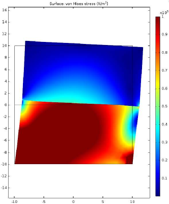
(a) Stresses $\sigma_{eq}^{+},\sigma_{eq}^{-}$ in the regions $\Omega^{+}\cup\Omega^{-}$

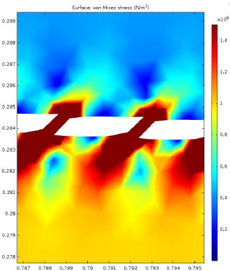
(b) Stresses $\sigma_{\varepsilon,eq}$ in the layer $\Omega_{\varepsilon}^{i}$

Figure 2: Simulation results

The equivalent von Mises stresses for macro– and (local) micro–problems are presented in Fig. 2. Fig. 2 (a) provides the solution of the equation (7.2)–(7.4) in macroscopic blocks and jumps in the equivalent von Mises stresses across the interface can be observed. Fig. 2 (b) shows the local $\varepsilon$–solution in the layer for $\varepsilon=0.004$.

Comparison results for chosen $\varepsilon$ are gathered in the Table 1.

$\varepsilon$	$\|[u_{\varepsilon,1}]-[u_{1}]\|$	$\|[u_{\varepsilon,2}]\|$	$\|\sigma^{+}_{\varepsilon,12}-\sigma^{+}_{12}\|$	$\|\sigma^{+}_{\varepsilon,22}-\sigma^{+}_{22}\|$
$0.1$	$2.9\cdot 10^{-5}$	$3\cdot 10^{-5}$	1.05	1.1
$0.02$	$2.5\cdot 10^{-5}$	$1.6\cdot 10^{-5}$	0.59	0.6
$0.004$	$7.6\cdot 10^{-6}$	$7.7\cdot 10^{-6}$	0.3	0.1

Table 1: Norms of the residual

Acknowledgements. This work was supported by Deutsche Forschungsgemeinschaft (Grants No. OR 190/4–2 and OR 190/6–1).

References

- [1] G. Griso Decompositions of displacements of thin structures, J. Math. Pures Appl. 89, 199–223, 2008
- [2] G. Griso Asymptotic behavior of curved rods by the unfolding method, Math. Meth. Appl. Sci. 27: 2081-2110, 2004
- [3] D. Blanchard, A. Gaudiello, G. Griso Junction of a periodic family of elastic rods with a 3d plate. Part I, J. Math. Pures Appl. 88–1, 1–33, 2007
- [4] D. Blanchard, A. Gaudiello, G. Griso Junction of a periodic family of elastic rods with a 3d plate. Part II, J. Math. Pures Appl. 88–2, 149–190, 2007
- [5] L. Trabucho, J. M. Viano Mathematical Modelling of Rods, Hand–book of Numerical Analysis, vol. 4, North–Holland, Amsterdam, 1996
- [6] D. Cioranescu, A. Damlamian, G. Griso Periodic unfolding and homogenization, C. R. Acad. Sci. Paris Sér. I Math. 338 (2004) 261–266
- [7] D. Cioranescu, A. Damlamian and G. Griso The periodic unfolding method in homogenization, SIAM J. of Math. Anal. Vol. 40, 4 (2008), 1585–1620
- [8] O. A. Oleinik, A. S. Shamaev, G. A. Yosifan Mathematical Problems in Elasticity and Homogenization, North Holland, 1992
- [9] D. Cioranescu, A. Damlamian, G. Griso, D. Onofrei The periodic unfolding method for perforated domains and Neumann sieve models, J. Math. Pures Appl. 89, 2008
- [10] M. Neuss–Radu and W. Jäger Effective transmission conditions for reaction-diffusion processes in domains separated by an interface, SIAM J. Math. Anal. Vol. 39, No. 3, pp. 687–720, 2007
- [11] G. Geymonat, F. Krasucki, S. Lenci Mathematical analysis of a bonded joint with a soft thin adhesive, Math. Mech. Solids, Vol. 4, (1999), pp. 201–225
- [12] S. Pastukhova Homogenization of problems of elasticity theory on periodic box and rod frames of critical thickness, Journal of Mathematical Sciences, Springer New York, Vol. 130, 5, 4954–5004, 2005
- [13] V. V. Zhikov, S. E. Pastukhova Homogenization for elasticity problems on periodic networks of critical thickness, Sbornik: Mathematics, Vol. 194, 5, 697, 2003
- [14] G. P. Panasenko Multiscale Modelling for Structures and Composites, Springer, 2005