Giant Anomalous Hall Effect in the Chiral Antiferromagnet Mn3Ge
Abstract
The external field control of antiferromagnetism is a significant subject both for basic science and technological applications. As a useful macroscopic response to detect magnetic states, the anomalous Hall effect (AHE) is known for ferromagnets, but it has never been observed in antiferromagnets until the recent discovery in Mn3Sn. Here we report another example of the AHE in a related antiferromagnet, namely, in the hexagonal chiral antiferromagnet Mn3Ge. Our single-crystal study reveals that Mn3Ge exhibits a giant anomalous Hall conductivity cm-1 at room temperature and approximately cm-1 at 5 K in zero field, reaching nearly half of the value expected for the quantum Hall effect per atomic layer with Chern number of unity. Our detailed analyses on the anisotropic Hall conductivity indicate that in comparison with the in-plane-field components and , which are very large and nearly comparable in size, we find obtained in the field along the axis is found to be much smaller. The anomalous Hall effect shows a sign reversal with the rotation of a small magnetic field less than 0.1 T. The soft response of the AHE to magnetic field should be useful for applications, for example, to develop switching and memory devices based on antiferromagnets.
I. Introduction
The anomalous Hall effect (AHE) is one of the best-studied transport properties of solid. Since its discovery in 1880, the effect is known to be proportional to magnetization, and, thus, the zero field AHE has been observed only in ferromagnets Chien and Westgate (1980); Nagaosa et al. (2010). Hypothetically, however, since intrinsic AHE arises owing to fictitious fields due to Berry curvature, it may appear in spin liquids and antiferromagnets without spin magnetization in certain conditions, even with a large Hall conductivity comparable with the quantum Hall effect (QHE) Shindou and Nagaosa (2001); Metalidis and Bruno (2006); Martin and Batista (2008); Yang et al. (2011); Ishizuka and Motome (2013); Chen et al. (2014); Kübler and Felser (2014). Indeed, a spontaneous Hall effect has been observed in recent experiments in the spin liquid Pr2Ir2O7 Machida et al. (2010) and the antiferromagnet Mn3Sn Nakatsuji et al. (2015). Nonetheless, the zero-field AHE observed to date reached only a few orders of magnitude lower value than the QHE per atomic layer.
In recent years, antiferromagnets have attracted an increasing amount of attention due to the useful properties, in particular, for spintronics Núñez et al. (2006); Shick et al. (2010); MacDonald and Tsoi (2011); Park et al. (2011); Marti et al. (2014); Gomonay and Loktev (2014). In contrast with ferromagnets that have been mainly used to date Chappert et al. (2007), antiferromagnets are much more insensitive against magnetic field perturbations, providing stability for the data retention. In addition, antiferromagnets produce almost no stray fields that perturb the neighboring cells, removing an obstacle for high-density memory integration. Moreover, antiferromagnets have much faster spin dynamics than ferromagnets, opening avenues for ultrafast data processing.
On the other hand, to develop antiferromagnetic devices, it is necessary to find detectable macroscopic effects that can be changed by the rotation of the sublattice moments. Thus, if we can find an antiferromagnet that exhibits a large AHE at room temperature, it will be useful for switching and memory devices, as a large change in the Hall voltage clearly defines binary information.
In this article, we report the observation of a giant anomalous Hall conductivity in an antiferromagnet reaching approximately % of the layered quantum Hall effect with Chern number of unity. In particular, we show that the noncollinear antiferromagnet Mn3Ge isostructural to Mn3Sn exhibits strikingly large anomalous Hall conductivity in zero field of approximately 60 cm-1 at room temperature and approximately 380 cm-1 at 5 K. Moreover, the sign of the giant AHE can be softly flipped by the rotation of magnetic field, indicating that the direction of a fictitious field equivalent to more than T is tunable by a small external magnetic field less than 0.1 T. Thus, the AHE should be useful for applications, for example, to develop switching and memory devices based on antiferromagnets.
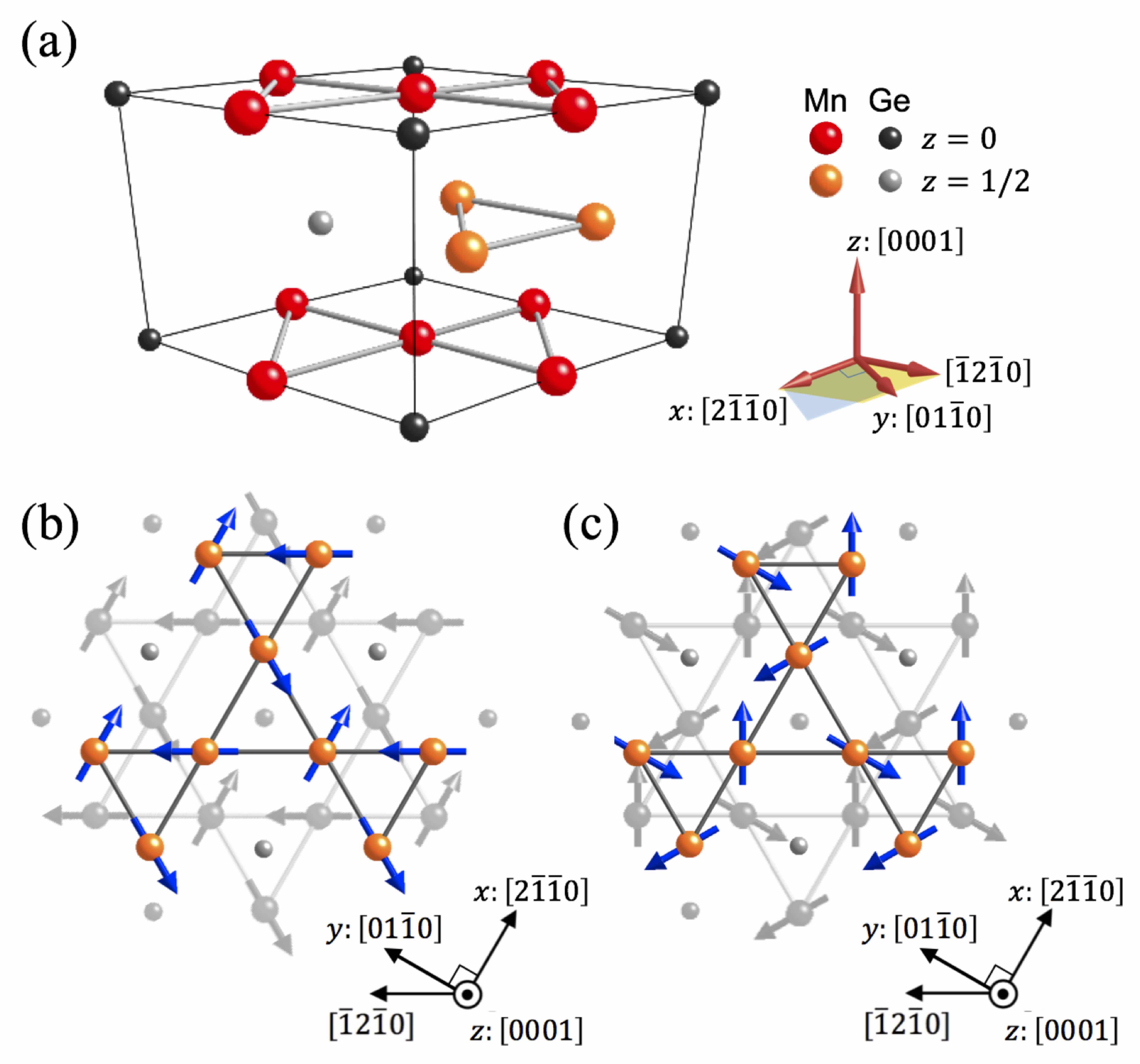
Mn3Ge is isostructural to Mn3Sn, which has Ni3Sn-type structure with the hexagonal symmetry [Fig. 1(a)]. The structure is stable only when there is excess Mn randomly occupying the Ge site. As a result, this phase exists over the range of Mn3.2Ge-Mn3.4Ge Yamada et al. (1988). The projection of the Mn atoms onto the basal plane is a triangular lattice made by a twisted triangular tube of face-sharing octahedra. In each plane, the Mn atoms form a “breathing” type of a Kagome lattice (an alternating array of small and large triangles), and the associated geometrical frustration leads to a noncollinear 120∘ spin ordering of the magnetic moments approximately /Mn below the Néel temperature of approximately 380 K, similarly to Mn3Sn Nagamiya et al. (1982); Tomiyoshi and Yamaguchi (1982). Contrary to the usual 120 degree order, all Mn moments lying in the - plane form a chiral spin texture with an opposite vector chirality owing to the Dzyaloshinskii-Moriya interaction [Figs. 1(b) and 1(c)]. This inverse triangular structure has the orthorhombic symmetry and induces an in-plane weak ferromagnetic (FM) moment of the order of approximately Mn, which is believed to arise from the spin canting toward the local easy axis along the direction Nagamiya et al. (1982); Tomiyoshi et al. (1983). This in-plane chiral magnetic phase is stable down to the lowest ’s Yamada et al. (1988), which allows us to observe a giant AHE at low temperatures, as we will discuss. In contrast, Mn3Sn has a low- noncoplanar magnetic phase at K, where the in-plane AHE is strongly suppressed Nakatsuji et al. (2015). In our study, single crystals with the composition of Mn3.05Ge0.95 (Mn3.22Ge) are mainly used and referred to as “Mn3Ge” for clarity (see Appendix A).
II. Results and Discussion
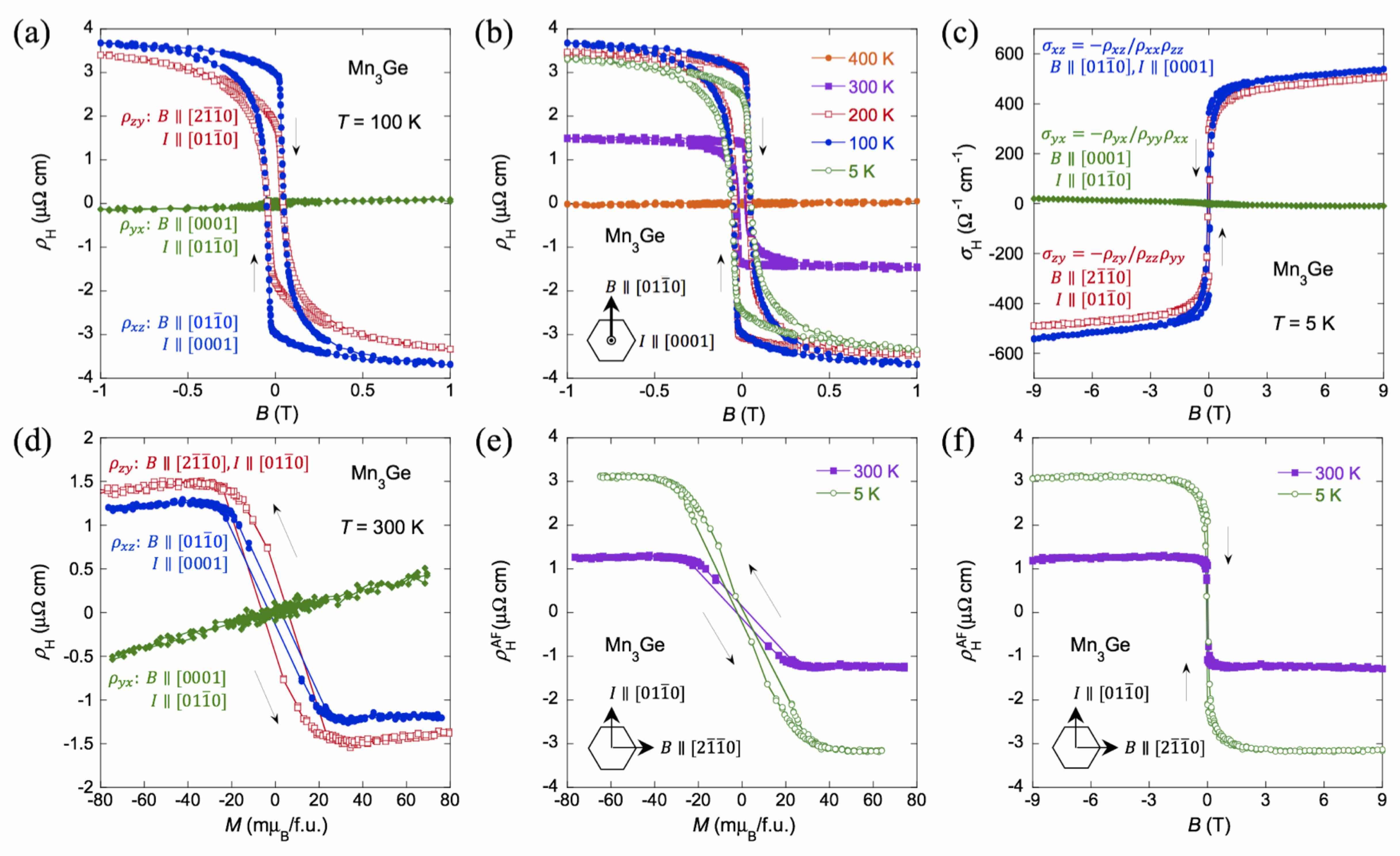
We first present our main experimental evidence for the giant anomalous Hall effect found in Mn3Ge. The Hall voltage is measured in the direction perpendicular to both the magnetic field and the electric current . Figure 2(a) shows the field dependence of the Hall resistivity obtained at 100 K in , , and with perpendicular to . It exhibits a clear hysteresis loop with a large change cm for comparable to Mn3Sn Nakatsuji et al. (2015). Besides, for free-electron gas with the carrier number estimated from (see below), it requires T for the ordinary Hall effect to reach the observed values of (see Appendix B). The hysteresis takes a similar small magnetic field to the Mn3Sn case; the coercivity increases from 300 Oe at 300 K to 600 Oe at 5 K [Fig. 2(b)], while it remains constant at approximately Oe for Mn3Sn Nakatsuji et al. (2015). This large anomaly is seen only in . The magnetoresistance (ratio) in this range (Appendix C) is less than 0.6 cm (0.4%), which is 1 order of magnitude smaller than . We further find that the hysteresis in is robust against a small change in the Mn concentration (see Appendix D).
To clarify the mechanism of transport properties in general, it is important to find the associated anisotropy. In the study of the anomalous Hall effect, however, the anisotropy is largely neglected. Since the longitudinal resistivity is anisotropic at low ’s (see below), for the estimate of the Hall conductivity, we employ the expression , where (see Appendix E). The results show a sharp hysteresis and reach large values of approximately at K and T [Fig. 2(c)]. This is nearly 4 times larger than in Mn3Sn Nakatsuji et al. (2015), and reaches approximately % of the value (approximately ) expected for a layered QHE as we discuss. In contrast, both and for exhibit a linear increase with except a very small hysteresis with cm and found around [Figs. 2(a) and 2(c)]. Significantly, similar sharp and anisotropic change as a function of field is seen at 300 K, as shown in Appendix F.
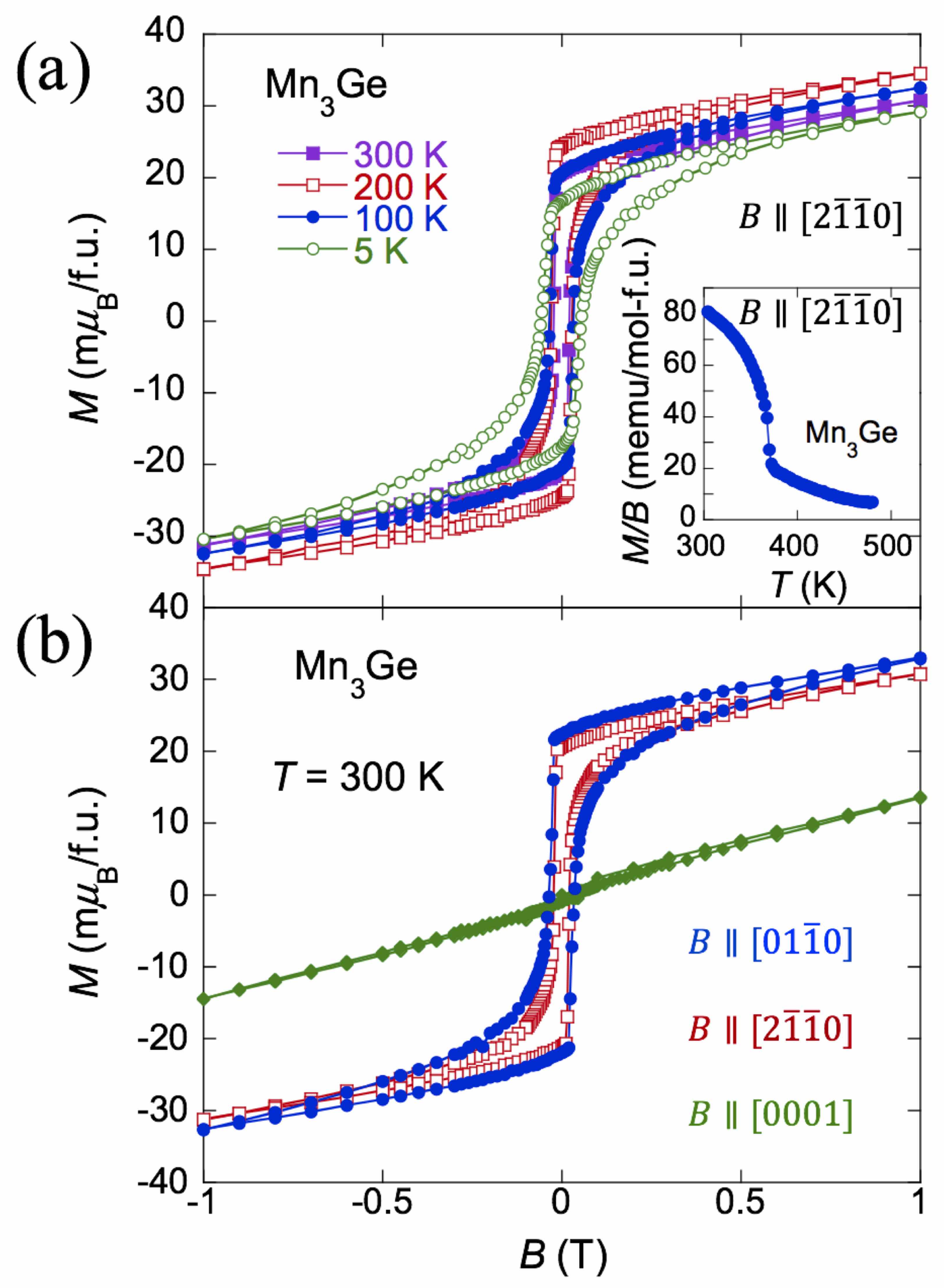
This sign change with a large jump of the anomalous Hall conductivity most likely indicates that the direction of the sublattice moments switch in response to the change in the external field by approximately 0.1 T, suggesting an extremely small energy scale associated with magnetocrystalline anisotropy Nagamiya et al. (1982); Tomiyoshi et al. (1983). Various spin configurations in the in-plane fields are shown in Appendix G. Indeed, a theoretical analysis reveals that the inverse triangular spin structure should have no in-plane anisotropy energy up to the fourth-order term Nagamiya et al. (1982); Tomiyoshi et al. (1983). Thus, the spin triangle should rotate easily, following the sign change of magnetic field. Here, we note that the in-plane weak FM moment is essential for the magnetic field control of the staggered moment axis. Indeed, the magnetization hysteresis curve obtained in at between 5 and 300 K reveals that a weak FM moment (- m/Mn) changes its direction with almost the same coercivity as observed in the Hall effect [Fig. 3(a)]. While the in-plane is almost isotropic, exhibiting clear hysteresis, for mainly shows a linear dependence except a very tiny FM component of approximately m/Mn [Fig. 3(b)]. The in-plane weak ferromagnetism appears below K as can be seen in the dependence of the susceptibility for [Fig. 3(a) inset].
The Hall resistivity is conventionally described as the sum of the normal and anomalous Hall effects, which are proportional to and , respectively. However, to characterize the spontaneous Hall effect seen in the noncollinear antiferromagnet Mn3Sn Nakatsuji et al. (2015), we find that the additional term is necessary, and its Hall resistivity can be written as,
| (1) |
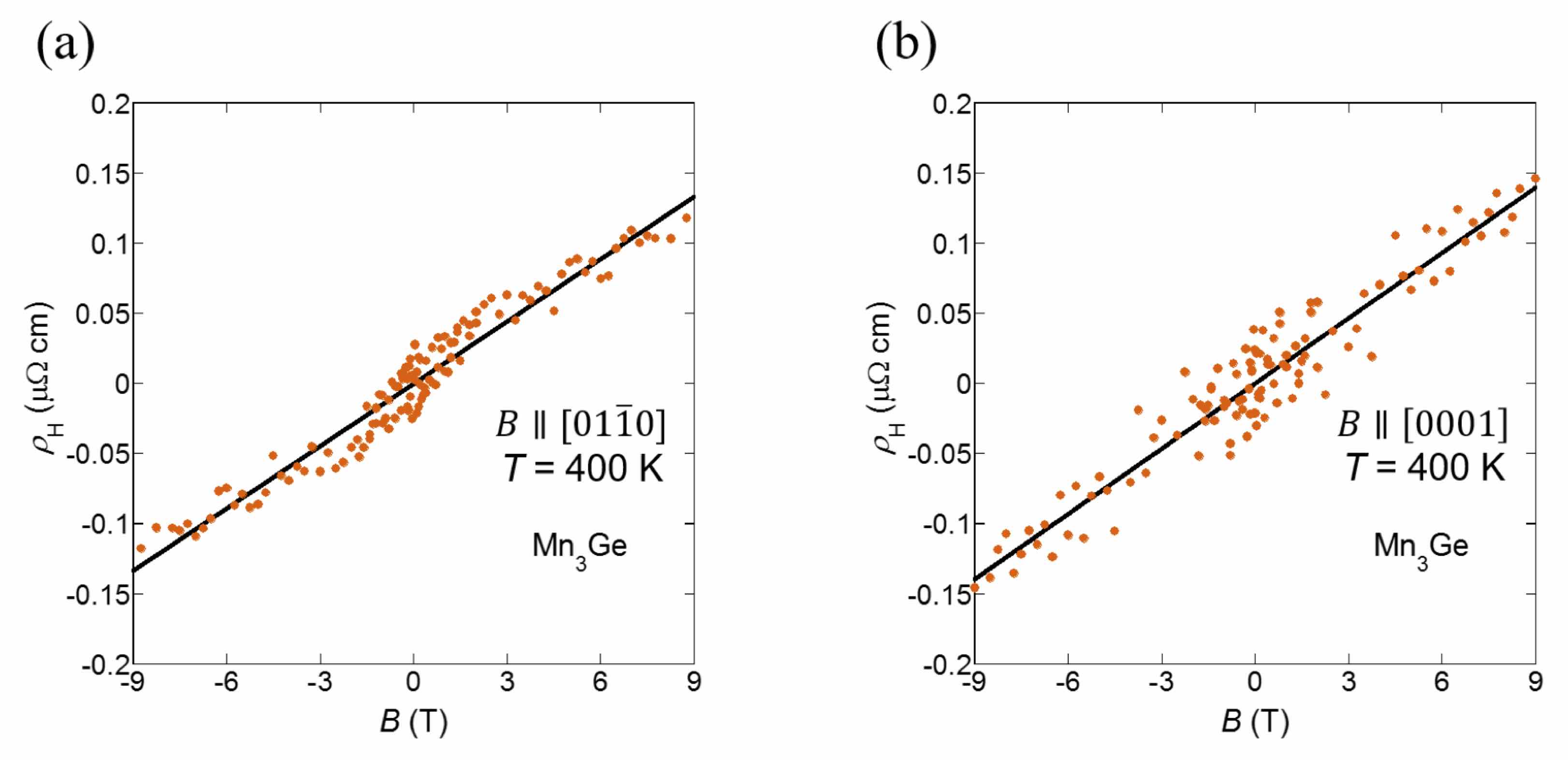
where and are the normal and anomalous Hall coefficients, respectively. Here, we examine if the same Eq. (1) may describe the AHE in Mn3Ge. The large zero-field component indicates that the AHE should dominate the Hall effect. To further confirm this, we estimate the normal Hall effect (NHE) using the field dependence of at 400 K in the paramagnetic regime, where the in-plane and out-of-plane both linearly increase with with nearly the same slope (see Appendix B). The slope yields cm/T, which provides the upper limit of the estimate of and thus indicates that the NHE contribution is negligibly small and the AHE dominates (see Appendix B).
Next, to check the magnetization dependence of the AHE, we plot vs , taking the magnetic field as an implicit parameter [Fig. 2(d)]. For the -axis component, linearly increases with and, thus, . For the - plane component, in a high-field regime also increases linearly with with a positive slope, . However, in the low-field regime where shows a hysteresis with a spontaneous component, the Hall resistivity also exhibits a hysteresis loop as a function of . This is the same behavior as seen in Mn3Sn Nakatsuji et al. (2015) and indicates that has an additional spontaneous term as described in Eq. (1). Notably, the magnetization in these two field regions has qualitatively different field response. The magnetization in the low-field regime corresponds to the weak ferromagnetism and exhibits hysteresis, while the high-field region with the small slope has the linear in-field increase, which most likely comes from the field-induced canting of the AF sublattices [Figs. 3(a) and 3(b)].
By using and the high-field slope, , estimated above, we obtain as a function of both and [Figs. 2(e) and 2(f)]. Unlike the conventional AHE, is not linearly dependent on or . Given that the neutron-diffraction measurements and theoretical analysis show that the staggered moments of the chiral noncollinear spin structure freely rotate following the in-plane field Nagamiya et al. (1982); Tomiyoshi et al. (1983), the large jump of with a sign change in should come from the switching of the staggered moment direction.
Normally, the AHE for a relatively resistive conductor is known to be proportional to the resistivity squared, Nagaosa et al. (2010). Thus, here we introduce the normalized parameter . For FM conductors, is independent of field and takes a value of the order of - V-1 Nagaosa et al. (2010); Nakatsuji et al. (2015). In high magnetic fields, of Mn3Ge indeed takes a constant value of approximately (300 K), (5 K) similar to ferromagnets Nakatsuji et al. (2015). However, for the zero-field spontaneous component, we find strikingly large values (300 K), (5 K) for . The extremely large value indicates that a distinct type of mechanism works here for the spontaneous Hall effect.
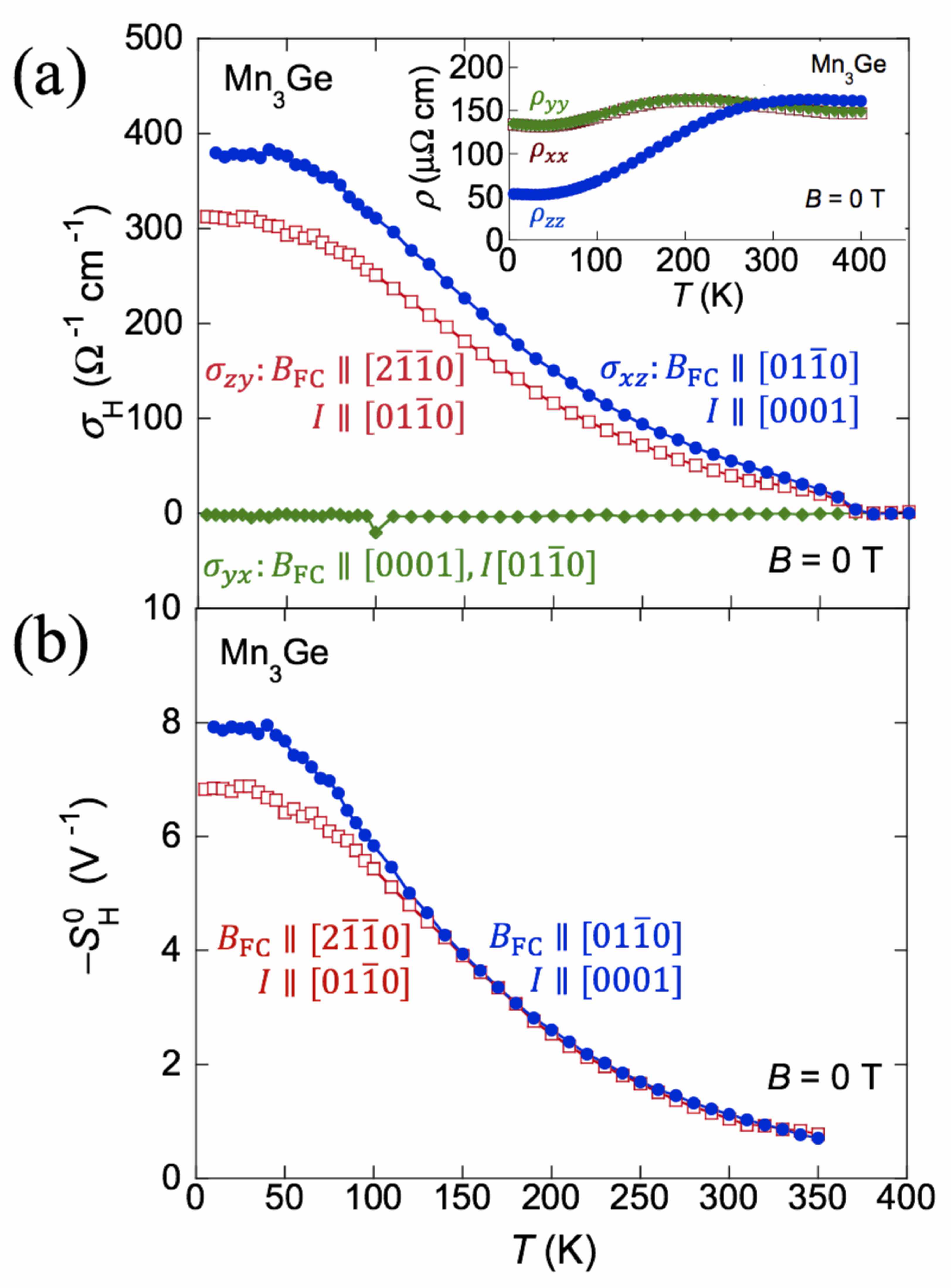
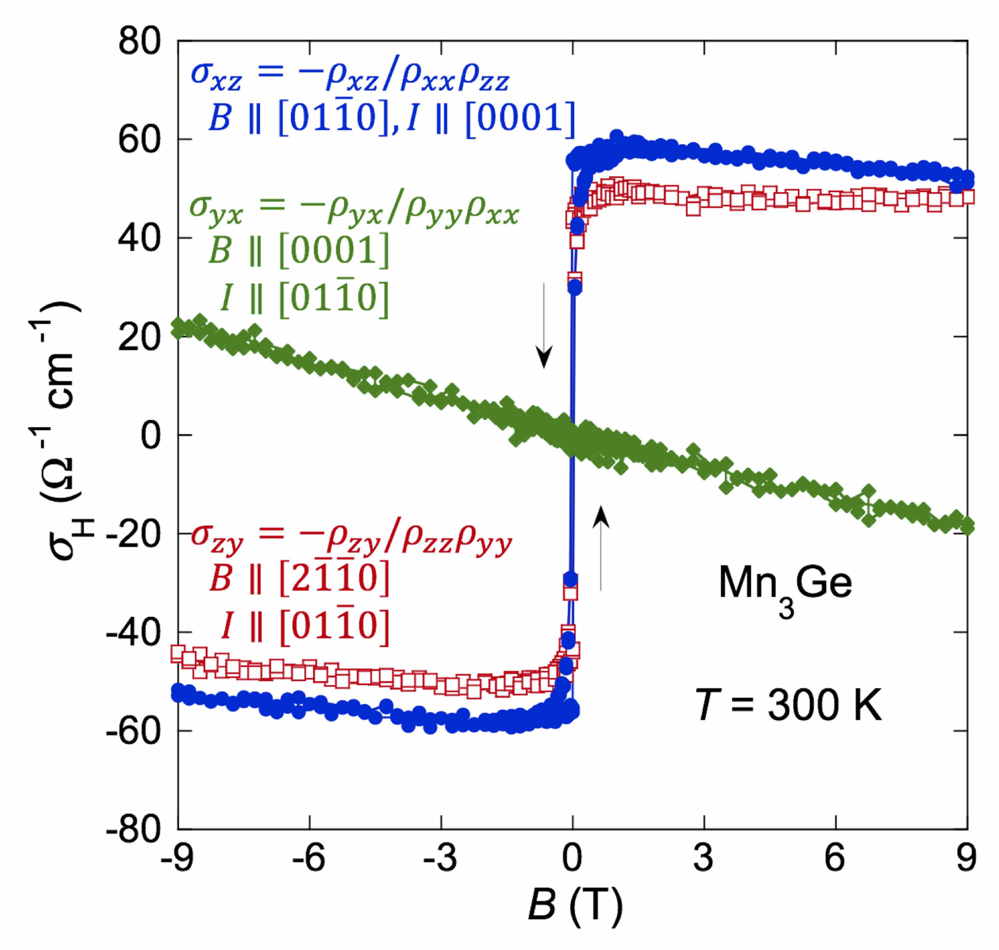
The temperature evolution of the spontaneous component of the AHE is examined by measuring the zero-field Hall resistivity and longitudinal resistivity on heating. They are concomitantly measured in the FC condition, namely, after cooling the sample under a magnetic field T from 350 K down to 5 K and consecutively setting at 5 K (see Appendix A). Figure 4(a) shows the dependence of the zero-field Hall conductivity ). The in-plane field components obtained after the Hall resistivity measurements in the FC condition in with and for and show nearly isotropic, large values reaching and cm-1 at K, respectively. Both and retain almost the same values up to approximately K where they start decreasing on heating. At 300 K, they remain nearly isotropic with cm-1 and cm-1 (see Appendix F), and finally vanish at K. In contrast, for and is less than 4 cm-1 and remains much smaller than and at all .
Similarly, the longitudinal resistivity as a function of exhibits anisotropic behaviors [Fig. 4(a) inset]; the in-plane components with and overlap on top, peaking at 200 K and having relatively large residual resistivity cm, while the out-of-plane component has a broad maximum at 300 K and shows a more conductive behavior with cm. To estimate , we also measure in zero field after the same FC procedure using the same sample as those used for the Hall effect measurements. The in-plane field components of are also found nearly isotropic [Fig. 4(b)], reaching a large value V-1 at 5 K, 2 orders of magnitude larger than the values known for the conventional AHE Nagaosa et al. (2010); Nakatsuji et al. (2015).
The observed giant spontaneous Hall effect in an antiferromagnet is striking and indicates an unusual mechanism of the AHE. One can discuss the possible AHE based on a symmetry argument. The inverse chiral triangular spin structure reduces the symmetry of the lattice from the hexagonal to orthorhombic and, thus, may induce not only the weak ferromagnetism but the AHE in the - plane. A numerical calculation using a different spin structure from the experimentally observed one indicates that the AHE can be large for Mn3Ge Kübler and Felser (2014). The AHE is given by the Brillouin zone integration of the Berry curvature Xiao et al. (2010), and the significant contribution is found from the band-crossing points called Weyl points Wan et al. (2011); Burkov and Balents (2011). The large size of the observed anomalous Hall conductivity for in-plane field reaching approximately - cm-1 under zero field has a similar magnitude as the theory, but the theory finds much more anisotropic AHE, as summarized in Table 3 in Appendix H Kübler and Felser (2014). The disagreement should come from the fact that the calculation in Ref. Kübler and Felser (2014) was made using spin structures different from what is observed in experiment Nagamiya et al. (1982); Tomiyoshi and Yamaguchi (1982); Tomiyoshi et al. (1983).
Theoretically, the anomalous Hall conductivity of a 3D system can reach a value as large as the one known for a layered 3D QHE, which has been proposed to appear in the systems called Chern insulators. Notably, the zero-field AHE observed in Mn3Ge reaches nearly half of cm-1, a value expected for a 3D QHE with Chern number of unity where the pair of Weyl points are separated by the reciprocal lattice vector G Yang et al. (2011); Turner and Vishwanath (2013). The fact that the sizes of and are comparable suggests that the separation between the Weyl points must be similar to each other for the cases of and . On the other hand, the origin of the much smaller than the in-plane field components and can be very small spin canting toward the axis and is a subject for future investigation.
III. Conclusion
The large AHE observed in Mn3Ge at room temperature may be significantly useful for various applications. In the field of spintronics, intensive studies have been made to find an antiferromagnet that serves as the active material for next-generation memory devices Núñez et al. (2006); Shick et al. (2010); MacDonald and Tsoi (2011); Park et al. (2011); Marti et al. (2014); Gomonay and Loktev (2014). In contrast with ferromagnets that have been mainly used for spintronics Chappert et al. (2007), antiferromagnets have robust stability against magnetic field perturbation and produce vanishingly small stray fields, thus, allowing high-density memory integration. The observed giant AHE in the chiral antiferromagnet Mn3Ge with a very small magnetization indicates that the material has a large fictitious field (equivalent to T) in the momentum space without producing almost any perturbing stray fields. The fact that the large fictitious field may be readily controlled by the application of a low external field indicates that the antiferromagnet will be useful, for example, to develop various switching and memory devices.
acknowledgments
Acknowledgements.
We thank Tomoya Higo, Muhammad Ikhlas, Hidetoshi Fukuyama, and Ryotaro Arita for useful discussions. This work is partially supported by PRESTO and CREST, JST, Grants-in-Aid for Scientific Research (Grants No. 25707030 and No.16H02209), by Grants-in-Aids for Scientific Research on Innovative Areas (Grants No. 15H05882 and No. 15H05883), and the Program for Advancing Strategic International Networks to Accelerate the Circulation of Talented Researchers (Grant No. R2604) from JSPS.| Mn3+xGe1-x () | Å3 | ||||
| lattice parameters (Spacegroup : ) | Å | Å | Å | ||
| Atom | Wyckoff position | Occupancy | |||
| Mn | 6h | 0.833(1) | 0.666(2) | 1/4 | 1 |
| Ge/Mn | 2c | 1/3 | 2/3 | 1/4 | (0.95/0.05) |
Note added.—After the completion of our work, we became aware of a similar work by Nayak et al. Nayak et al. (2015). The strong anisotropy for the in-plane field configuration in the Hall conductivity in Ref. Nayak et al. (2015) is inconsistent with our results. This most likely comes from the fact that we take account of the observed anisotropy of the longitudinal resistivity in the analysis of the Hall conductivity, as detailed in Appendix E.
Appendix A: Experiment
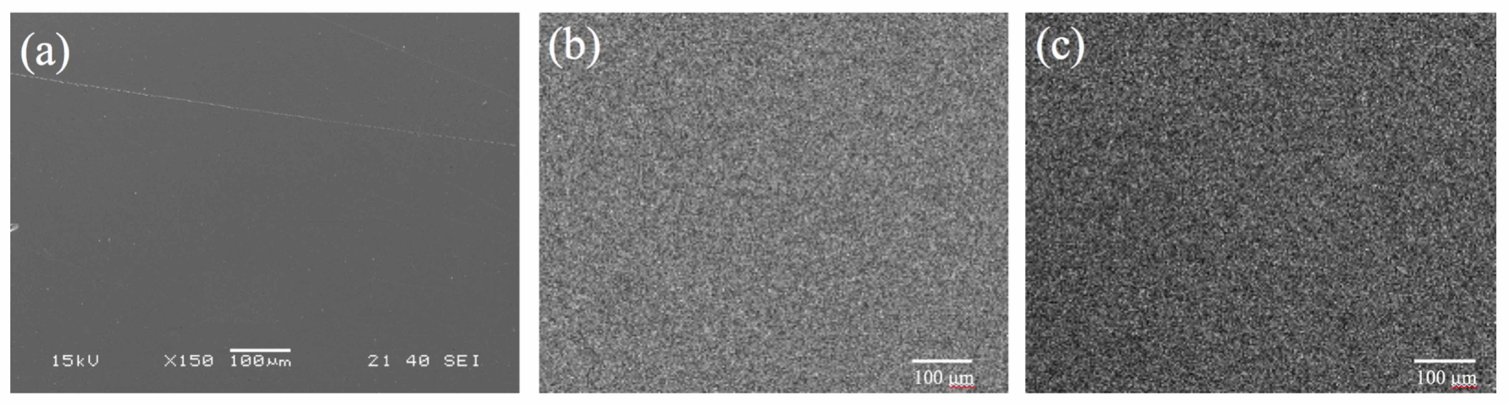
Polycrystalline samples are prepared by arc melting the mixtures of manganese and germanium in a purified argon atmosphere. Excess manganese (12 mol %) over the stoichiometric amount is added to compensate the loss during the arc melting and the crystal growth. The obtained polycrystalline materials are used for crystal growth by the Czochralski method using a commercial tetra-arc furnace (TAC-5100, GES). Subsequently, the sample is annealed for three days at 860 and quenched in water in order to remove the low-temperature phase, which has the tetragonal Al3Ti-type structure. Our SEM EDX (scanning electron microscopy with energy-dispersive x-ray spectroscopy) analysis for single crystals indicates that Mn3Ge is the bulk phase, and we find that the composition of the single crystals is Mn3.05Ge0.95 (Mn3.22Ge). Our single-crystal and powder x-ray measurements at 300 K confirm the majority of the hexagonal phase () of Mn3Ge with a small inclusion of the tetragonal phase whose volume fraction is less than 1%. This is consistent with our observation of a ferromagnetic component of approximately /f.u. in the magnetization curve under [Fig. 3(b) in the main text], taking account of the fact that the tetragonal phase is ferrimagnetic and has the net magnetization of /f.u. at room temperature Kurt et al. (2012). Rietveld analysis is made for the hexagonal phase of Mn3Ge and the associated results shown in Table 1 agree with those in the literature Niida et al. (1993). Figure 5 shows the SEM EDX mapping of a polished surface of a Mn3Ge single crystal. The EDX mapping images for Mn and Ge show that Mn and Ge are homogeneously mixed. In this paper, we mainly report the results on the crystal whose composition is Mn3.05Ge0.95 (Mn3.22Ge), and we refer to the crystal as “Mn3Ge” for clarity throughout the paper. On the other hand, in order to investigate the composition dependence of the Hall resistivity [Appendix D, Fig. 9], we also grow a single crystal whose composition is Mn3.07Ge0.93 (Mn3.32Ge).
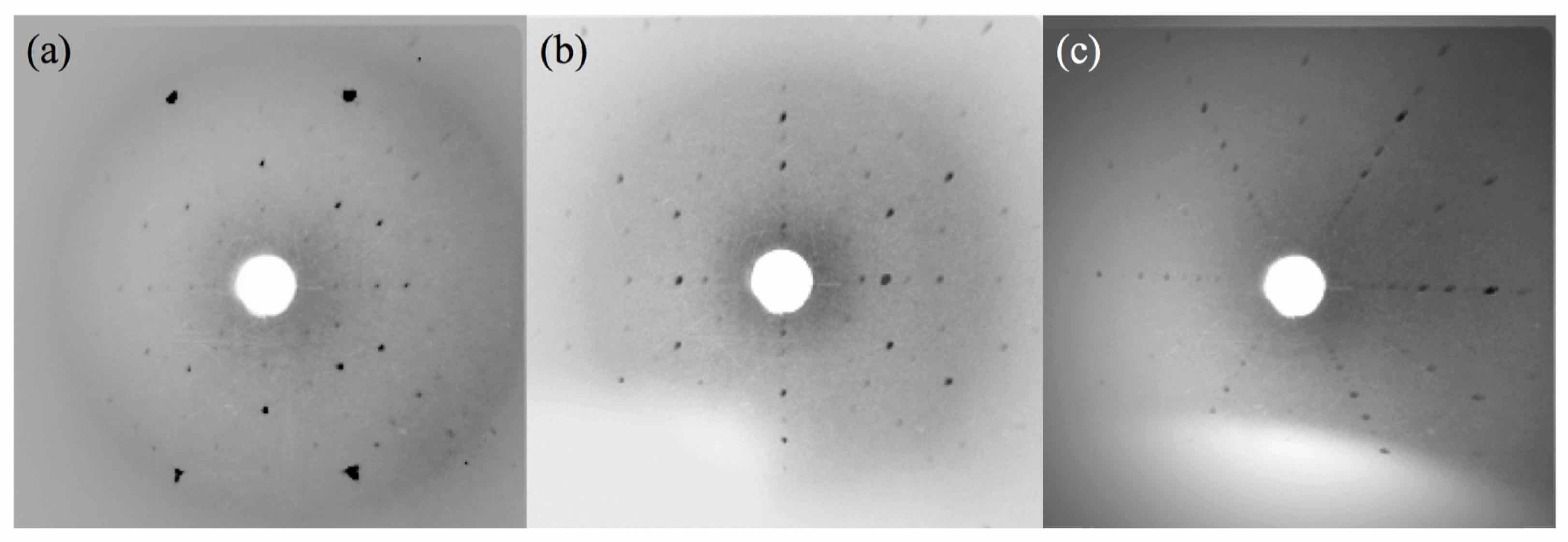
We measure the resistivity and magnetization using annealed single crystals after making a bar-shaped sample through the alignment made by using a Laue diffractometer (Fig. 6). We perform the magnetization measurements using a commercial superconducting quantum-interface-device magnetometer (MPMS, Quantum Design). We measure both longitudinal and Hall resistivities by a standard four-probe method using a commercial measurement system (PPMS, Quantum Design). In all the measurements, directions of the magnetic field, electric current, and Hall voltage are set perpendicular to each other.
We estimate the zero-field component of the anomalous Hall effect shown in Fig. 4 in the main text by the following method. We cool down samples from 400 K down to 5 K under a field of T ( T), and, subsequently, at 5 K, we decrease the field down to T ( T) without changing the sign of . Then, we measure the Hall voltage () in zero field at various temperatures on heating after stabilizing temperature at each point. To remove the longitudinal resistance component induced by the misalignment of the Hall voltage contacts, we estimate the zero-field component of the Hall resistance as . Here, is the electric current. Different samples are used for each field-cooling configuration shown in Fig. 4 in the main text. We measure the longitudinal resistivity at zero field concomitantly in the same procedures as those used for the Hall resistivity measurements. In addition, the zero-field longitudinal resistivity is measured using neighboring parts cut from the same crystal, and all the results and their anisotropy are consistent with those in Fig. 4(a) inset within an error bar of 10%. We also measure the zero-field remanent magnetization using the same field-cooling procedures, and the same samples as used in both longitudinal and Hall resistivity measurements.
Appendix B: Estimate of carrier concentration and fictitious field
The field dependence of the Hall resistivity at 400 K was obtained after subtracting the longitudinal resistivity component. Figures 7(a) and 7(b), respectively, show the Hall resistivity versus measured in and obtained at 400 K, which we find almost the same as each other. Black solid lines indicate linear fits yielding the slope cm/T for both orientations. Given a field-induced AHE contribution, this value of provides the upper limit of the estimate of the normal Hall coefficient and, thus, corresponds to the lower bound for the carrier concentration, namely, /Mn. The fictitious magnetic field corresponding to Berry curvature in space can be estimated using , where cm/T is used as the upper limit of the normal Hall coefficient . For example, since at 5 K [Fig. 2(f) in the main text], the fictitious field should be higher than approximately .

Appendix C: Field dependence of the longitudinal resistivity
| Concomitantly measured and | data used for | |
| in Fig. 2(c) | and | : 5 K data in Fig. 4(a) inset |
| in Fig. 2(c) | and | : 5 K data in Fig. 4(a) inset |
| in Fig. 2(c) | and | : 5 K data in Fig. 4(a) inset |
| in Fig. 4(a) | and | : -dependent data in Fig. 4(a) inset |
| in Fig. 4(a) | and | : -dependent data in Fig. 4(a) inset |
| in Fig. 4(a) | and | : -dependent data in Fig. 4(a) inset |
| in Fig. 10 | and | : 300 K data in Fig. 4(a) inset |
| in Fig. 10 | and | : 300 K data in Fig. 4(a) inset |
| in Fig. 10 | and | : 300 K data in Fig. 4(a) inset |
Over all temperature regions, a very small magnetoresistance is observed for all the in-plane and out-of-plane field directions. We find the magnetoresistance ratio to be much less than 1% and the associated resistivity is less than 10% of the Hall resistivity change. For example, in Fig. 8, we show the magnetoresistance ratio at various temperatures in the magnetic field with .
Appendix D: Composition dependence of the Hall resistivity
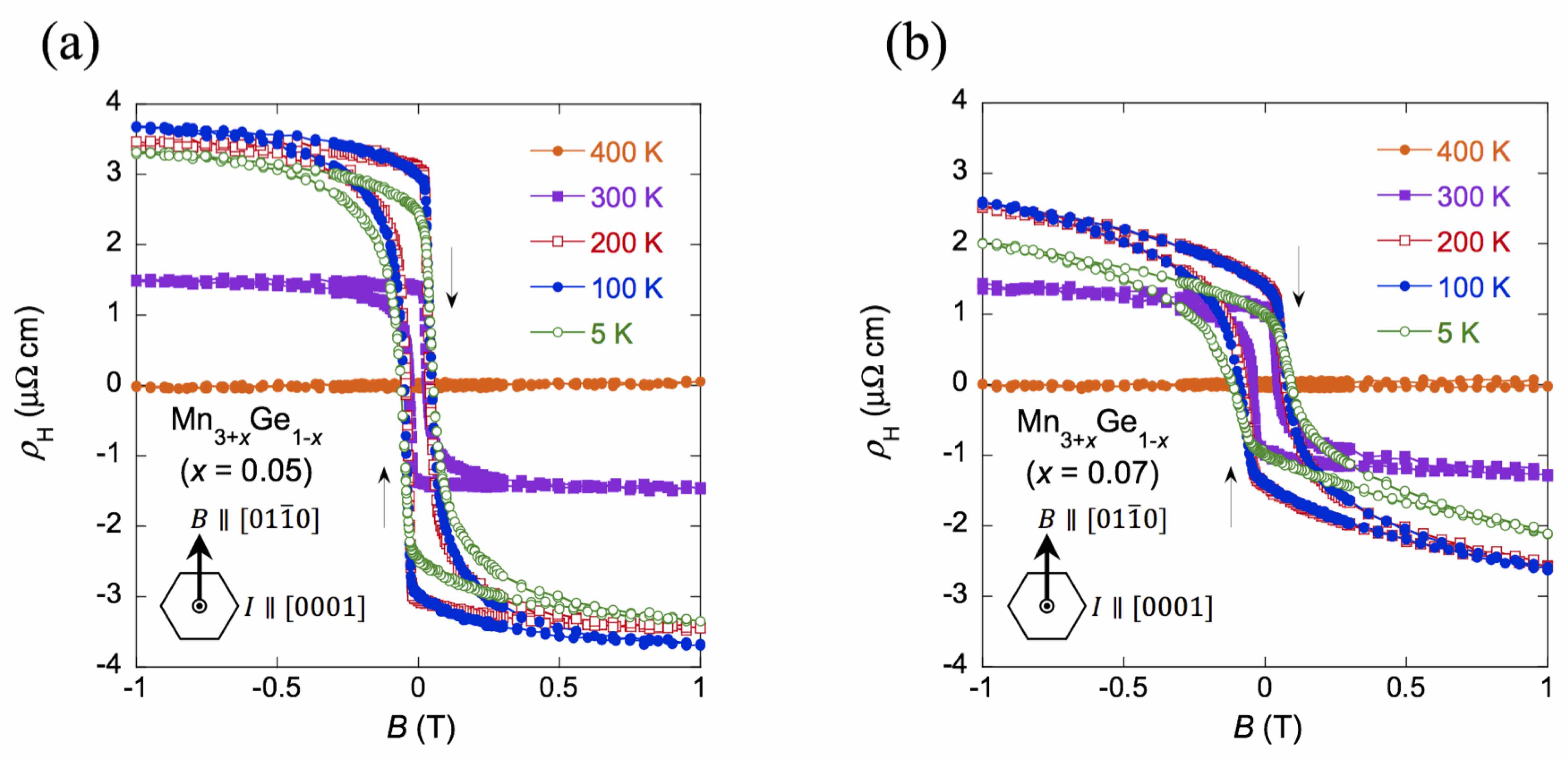
We find a large difference in the Hall resistivity at T between Mn3.05Ge0.95 and Mn3.07Ge0.93, as shown in Fig. 9. The difference in becomes larger with lowering temperature. For example, at zero field, the Hall resistivity at 5 K in Mn3.05Ge0.95 is twice larger than in Mn3.07Ge0.93. On the other hand, a similar magnitude is seen in for the results obtained above K. The coercivity increases with from approximately Oe () to approximately Oe (), indicating that the amount of the lattice defects and disorder increases with more excess of Mn.
Appendix E: Estimate of anisotropic Hall conductivity
The Hall conductivity is estimated as taking account of the observed anisotropy of the longitudinal resistivity, where or . For this analysis, two sets of the transport results are necessary (see Table 2). One is the Hall resistivity and the longitudinal resistivity (), both of which are concomitantly measured as described in Appendix A. The other is the longitudinal resistivity () for the vertical direction to (). To estimate the intrinsic anisotropy, both and are measured using the same sample or neighboring parts cut from the same crystal, as we describe above. Because of the anisotropy in the longitudinal resistivity, can be overestimated or underestimated from the one using the above equation if we calculate the Hall conductivity as . For example, in our measurements, reaches at K, and this is more than twice a larger value than estimated using anisotropic longitudinal resistivity in the same range.
| Material | Spin configuration | [K] | |||
|---|---|---|---|---|---|
| -Mn3Ge (This work) | 5 | ||||
| 100 | |||||
| 200 | |||||
| 300 | |||||
| -Mn3Ge (Theoretical work Kübler and Felser (2014)) | Fig. 2, Ref. Kübler and Felser (2014) | ||||
| Fig. 3(b), Ref. Kübler and Felser (2014) | |||||
| Fig. 5(c), Ref. Kübler and Felser (2014) | |||||
| Fig. 7, Ref. Kübler and Felser (2014) | |||||
| Fig. 7, Ref. Kübler and Felser (2014)∗ |
Appendix F: Anisotropy in field dependence of the Hall conductivity at 300 K
The field dependence of the Hall conductivity at 300 K for the field along the - plane and the axis is shown in Fig. 10. For the in-plane field, at 300 K is nearly isotropic, similar to the results at 5 K in Fig. 2(c) in the main text.
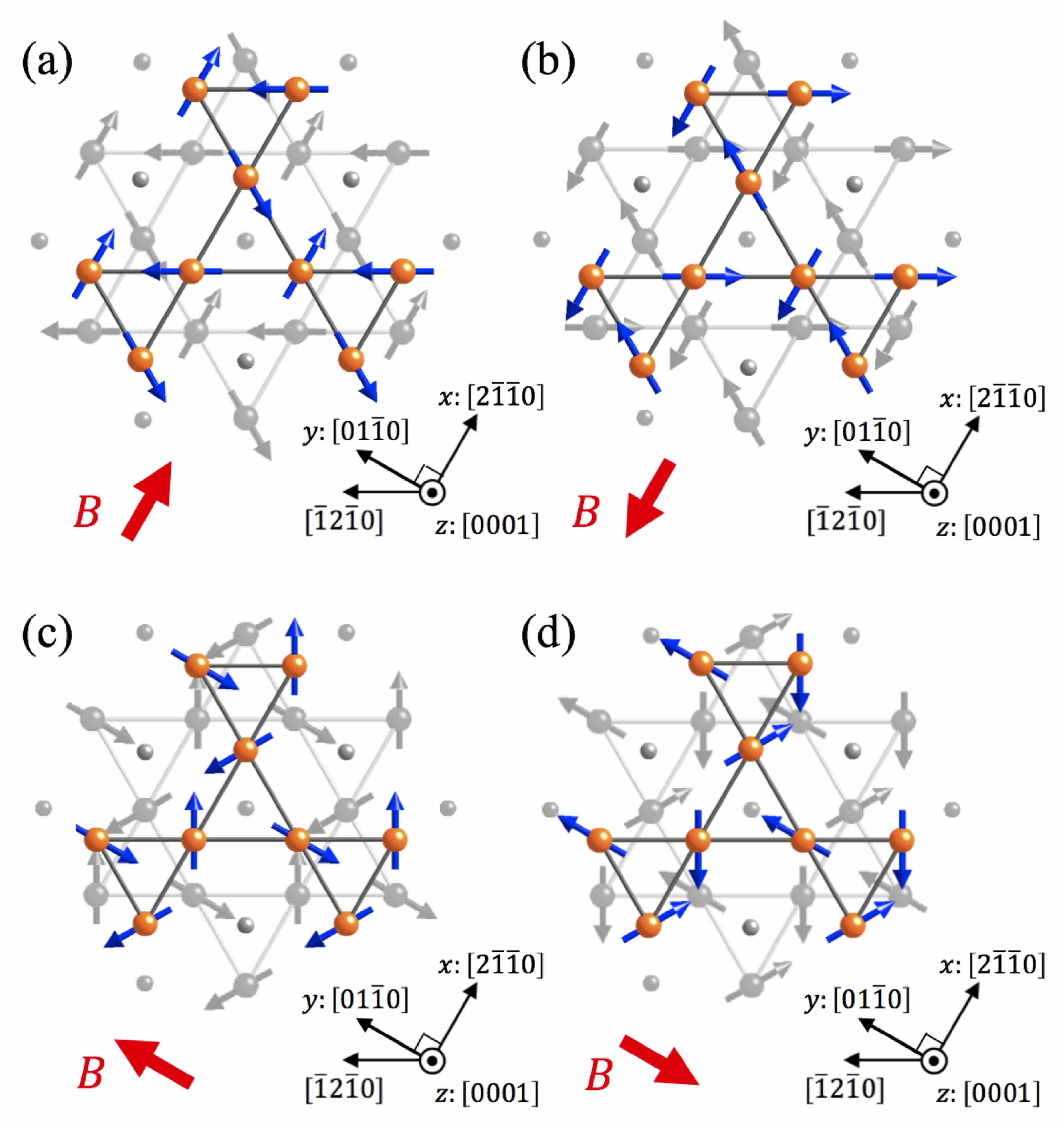
Appendix G: Spin configurations in in-plane magnetic field
When the magnetic field is applied along the in-plane directions and , the change in the spin configuration occurs from the one in Fig. 11 (a) to the other in Fig. 11(b), and from Fig. 11(c) to Fig. 11(d), respectively. The corresponding jumps in the Hall signal and magnetization are observed as a function of field as shown in Figs. 2 and 3 in the main text, respectively.
Appendix H: Comparison between theoretical calculations and experimental results
In Table 3, we compare our results of the anomalous Hall conductivity of Mn3Ge with those calculated for spin configurations by Kübler and Felser Kübler and Felser (2014) (Figs. 2, 3, 5, and 7). While the order of magnitude is similar, our results are different from their calculations in terms of the sign and anisotropy. It should be noted that spin configurations used in Ref. Kübler and Felser (2014) are not consistent with the results obtained from the neutron-diffraction measurements Nagamiya et al. (1982); Tomiyoshi et al. (1983).
References
- Chien and Westgate (1980) C. L. Chien and C. R. Westgate, The Hall Effect and Its Applications (Plenum, New York, 1980).
- Nagaosa et al. (2010) N. Nagaosa, J. Sinova, S. Onoda, A. H. MacDonald, and N. P. Ong, Rev. Mod. Phys. 82, 1539 (2010).
- Shindou and Nagaosa (2001) R. Shindou and N. Nagaosa, Phys. Rev. Lett. 87, 116801 (2001).
- Metalidis and Bruno (2006) G. Metalidis and P. Bruno, Phys. Rev. B 74, 045327 (2006).
- Martin and Batista (2008) I. Martin and C. D. Batista, Phys. Rev. Lett. 101, 156402 (2008).
- Yang et al. (2011) K.-Y. Yang, Y.-M. Lu, and Y. Ran, Phys. Rev. B 84, 075129 (2011).
- Ishizuka and Motome (2013) H. Ishizuka and Y. Motome, Phys. Rev. B 87, 081105 (2013).
- Chen et al. (2014) H. Chen, Q. Niu, and A. H. MacDonald, Phys. Rev. Lett. 112, 017205 (2014).
- Kübler and Felser (2014) J. Kübler and C. Felser, Europhys. Lett. 108, 67001 (2014).
- Machida et al. (2010) Y. Machida, S. Nakatsuji, S. Onoda, T. Tayama, and T. Sakakibara, Nature (London) 463, 210 (2010).
- Nakatsuji et al. (2015) S. Nakatsuji, N. Kiyohara, and T. Higo, Nature (London) 527, 212 (2015).
- Núñez et al. (2006) A. S. Núñez, R. A. Duine, P. Haney, and A. H. MacDonald, Phys. Rev. B 73, 214426 (2006).
- Shick et al. (2010) A. B. Shick, S. Khmelevskyi, O. N. Mryasov, J. Wunderlich, and T. Jungwirth, Phys. Rev. B 81, 212409 (2010).
- MacDonald and Tsoi (2011) A. H. MacDonald and M. Tsoi, Phil. Trans. R. Soc. A 369, 3098 (2011).
- Park et al. (2011) B. G. Park, J. Wunderlich, X. Marti, V. Holy, Y. Kurosaki, M. Yamada, H. Yamamoto, A. Nishide, J. Hayakawa, H. Takahashi, A. B. Shick, and T. Jungwirth, Nat. Mater. 10, 347 (2011).
- Marti et al. (2014) X. Marti, I. Fina, C. Frontera, J. Liu, P. Wadley, Q. He, R. J. Paull, J. D. Clarkson, J. Kudrnovský, I. Turek, J. Kuneš, D. Yi, J.-H. Chu, C. T. Nelson, L. You, E. Arenholz, S. Salahuddin, J. Fontcuberta, T. Jungwirth, and R. Ramesh, Nat. Mater. 13, 367 (2014).
- Gomonay and Loktev (2014) E. V. Gomonay and V. M. Loktev, Low Temp. Phys. 40, 17 (2014).
- Chappert et al. (2007) C. Chappert, A. Fert, and F. N. Van Dau, Nat. Mater. 6, 813 (2007).
- Nagamiya et al. (1982) T. Nagamiya, S. Tomiyoshi, and Y. Yamaguchi, Solid State Commun. 42, 385 (1982).
- Tomiyoshi et al. (1983) S. Tomiyoshi, Y. Yamaguchi, and T. Nagamiya, J. Magn. Magn. Mater. 31 - 34, 629 (1983).
- Yamada et al. (1988) N. Yamada, H. Sakai, H. Mori, and T. Ohoyama, Physica (Amsterdam) 149B, 311 (1988).
- Tomiyoshi and Yamaguchi (1982) S. Tomiyoshi and Y. Yamaguchi, J. Phys. Soc. Jpn. 51, 803 (1982).
- Xiao et al. (2010) D. Xiao, M.-C. Chang, and Q. Niu, Rev. Mod. Phys. 82, 1959 (2010).
- Wan et al. (2011) X. Wan, A. M. Turner, A. Vishwanath, and S. Y. Savrasov, Phys. Rev. B 83, 205101 (2011).
- Burkov and Balents (2011) A. A. Burkov and L. Balents, Phys. Rev. Lett. 107, 127205 (2011).
- Turner and Vishwanath (2013) A. M. Turner and A. Vishwanath, arXiv e-prints (2013), arXiv:1301.0330 [cond-mat.str-el] .
- Izumi and Momma (2007) F. Izumi and K. Momma, Solid State Phenom. 130, 15 (2007).
- Nayak et al. (2015) A. K. Nayak, J. E. Fischer, Y. Sun, B. Yan, J. Karel, A. C. Komarek, C. Shekhar, N. Kumar, W. Schnelle, J. Kübler, C. Felser, and S. S. P. Parkin, Sci. Adv. 2, e1501870 (2015).
- Kurt et al. (2012) H. Kurt, N. Baadji, K. Rode, M. Venkatesan, P. Stamenov, S. Sanvito, and J. M. D. Coey, Appl. Phys. Lett. 101, 132410 (2012), 10.1063/1.4754123.
- Niida et al. (1993) H. Niida, T. Hori, Y. Yamaguchi, and Y. Nakagawa, J. Appl. Phys. 73, 5692 (1993).