Mesons beyond the quark-antiquark picture

Abstract

The vast majority of mesons can be understood as quark-antiquark states. Yet, various other possibilities exists: glueballs (bound-state of gluons), hybrids (quark-antiquark plus gluon), and four-quark states (either as diquark-antidiquark or molecular objects) are expected. In particular, the existence of glueballs represents one of the first predictions of QCD, which relies on the nonabelian feature of its structure; this is why the search for glueballs and their firm discovery would be so important, both for theoretical and experimental developments. At the same time, many new resonances ($X,Y,$ and $Z$ states) were discovered experimentally, some of which can be well understood as four-quark objects. In this lecture, we review some basic aspects of QCD and show in a pedagogical way how to construct an effective hadronic model of QCD. We then present the results for the decays of the scalar and the pseudoscalar glueballs within this approach and discuss the future applications to other glueball states. In conclusion, we briefly discuss the status of four-quark states, both in the low-energy domain (light scalar mesons) as well as in the high-energy domain (in the charmonia region)

1 Introduction

A big part of the Particle Data Group [1] contains a list of strongly interacting and short-living resonances($\tau\sim 10^{-22}$ s), whose properties and decay channels were determined via many experimental collaborations in the last decades.

Quantum Chromodynamics (QCD) contains only quarks and gluons and is based on the invariance under local color transformations, denoted as $SU_{c}(3).$ There are 6 types (flavors) of quarks: the quarks $u,$ $d,$ $s$ are light with $m_{u}=1.8$-$3.0$ MeV$,m_{d}=4.5$-$5.3$ MeV, and $m_{s}=95\pm 5$ MeV, while the quarks $c,b,t$ are heavy with $m_{c}=1.275\pm 0.025$ GeV, $m_{b}=$ $4.18\pm 0.03$ GeV, and $m_{t}=173.2\pm 1.2$ GeV (mass values from [1]). Each quark flavor carries a color: reed, green, or blue. Moreover, there are 8 gluons. Each gluon appears as a color-anticolor state, such as red-antigreen. There is no colorless white gluon, explaining why there are only 8 of them.

QCD could not be analytically solved in its low-energy domain because perturbation theory does not apply: this is due to the fact that the running coupling constant increases for decreasing energy. A related property is confinement: only ‘white’ states, i.e. states which are invariant under local $SU_{c}(3)$ transformations, are realized in Nature. Colored objects, such as quarks and gluons (but also diquarks), are not states which hit our detectors.

Which are then the asymptotic states of QCD? They are called hadrons (hadrons means ‘thick’ in ancient greek). Two types of hadrons exist: mesons and baryons. For a proper definition of them, we need to introduce the baryon number: each quark, independently of its flavor and color, carries a baryon number $B_{q}=1/3$, while each gluon has a vanishing baryon number, $B_{g}=0$. Then the following general definitions apply:

Mesons are white states (i.e. invariant under color transformations) which have a vanishing total baryon number. Quark-antiquark states of the type $\left|\overline{q}q\right\rangle$, such as pions, kaons, etc., are mesons [2]. In fact: $B_{\overline{q}q}=B_{q}+B_{\overline{q}}=\frac{1}{3}-\frac{1}{3}=0$. They are regarded as conventional mesons, but they are not the only possibility [3]. Glueballs are mesonic states made solely of (two or more) gluons and are denoted as $\left|gg\right\rangle.$ They are a long-standing but not yet fulfilled promise of QCD. Glueballs are mesons because their baryon number is obviously zero, since each gluon is such. In addition, there are also mesonic tetraquark states made out of a diquark and an antidiquark, $\left|\left(\overline{q}\overline{q}\right)\left(qq\right)\right\rangle$, or mesonic molecular states $\left|\left(\overline{q}q\right)\left(\overline{q}q\right)\right\rangle.$ Hybrids are also outstanding candidates [4]: they are made of a quark-antiquark couple plus one (or more) gluon(s), $\left|\overline{q}qg\right\rangle.$ In general, each state made of $n$ quarks, $n$ antiquarks, and $m$ gluons has total baryon number equal to zero and is in principle a meson. Yet, while quark-antiquark states were measured in countless experiments, only very recently it was possible to confirm the existence of mesons beyond the quark-antiquark picture (four-quark states, either in the tetraquark or molecular-like picture and/or admixtures of them), see for instance [5, 6, 7]. For what concerns glueballs, some candidates exist (especially for the lightest scalar glueball), but the final verification of their existence has still to come.

Baryons are hadronic states with total baryon number $B=1$. Three-quark states $\left|qqq\right\rangle$, such as the neutron and the proton, are baryons. Also in this case, there are other possible configurations, such as pentaquarks $\left|(qq)(qq)\overline{q}\right\rangle$ (diquark-diquark-antiquark) and molecular-like objects as $\left|(qqq)\left(\overline{q}q\right)\right\rangle$, see the recent result in Ref. [8].

In these lectures we concentrate on mesons. In Sec. 2 we review some basic properties of the QCD Lagrangian (symmetries and large-$N_{c}$) as well as some general properties of conventional quark-antiquark mesons. In Sec. 3 we turn our attention to the construction of an effective hadronic model of QCD, the so-called extended Linear Sigma Model (eLSM). We present its building blocks in detail since the considerations leading to it are quite general and are based solely on symmetry. A primary element of the eSLM is the dilaton field, which is naturally linked to the scalar glueball. Glueballs are then studied in Sec. 4: the decays and the assignment of the scalar glueball are presented (the resonance $f_{0}(1710)$ is the most prominent candidate). Then, the branching ratios of a not-yet discovered pseudoscalar glueball are calculated. In Sec. 5 we move to four-quark objects. We first study the light scalar sector, where the resonances $f_{0}(500),$ $f_{0}(980),$ $a_{0}(980),$ and $K_{0}^{\ast}(800)$ are most probably not $\bar{q}q$ states; then we briefly discuss the status of $X,Y,$ and $Z$ states in the region between $3$-$5$ GeV, where recent experimental discoveries have nicely shown the existence of mesons which go beyond the quark-antiquark picture. Finally, in Sec. 6 we present our conclusions.

This work is based on two lectures given at the 55 Cracow School of Theoretical Physics (Zakopane, 2015). The most important original papers are Refs. [9, 10, 11, 12, 13, 14, 15] as well as my habilitation [16].

2 QCD and its symmetries, mesons, and large-$N_{c}$

2.1 Lagrangian of QCD and its symmetries

As a first step, we write the Lagrangian of $QCD$ for an arbitrary number of colors $N_{c}$ and quark flavors $N_{f}$ (see, for instance, [17]):

$$\mathcal{L}_{QCD} =\mathrm{Tr}\left[\overline{q}_{i}(i\gamma^{\mu}D_{\mu}-m_{i})q_{i}-\frac{1}{2}G_{\mu\nu}G^{\mu\nu}\right],\text{ }D_{\mu}=\partial_{\mu}-ig_{0}A_{\mu}\text{ ,}$$

$$G_{\mu\nu}^{a} =\partial_{\mu}A_{\nu}-\partial_{\nu}A_{\mu}-ig_{0}[A_{\mu},A_{\nu}],\text{ }A_{\mu}=A_{\mu}^{a}t^{a}\text{ ,}$$ (1)

where $a=1,...,N_{c}^{2}-1$ is the color index, $t^{a}$ are $N_{c}\times N_{c}$ matrices corresponding to the generators of $SU(N_{c})$ (see below), $f_{abc}$ are the structure constants of $SU(N_{c})$, and $i=1,...,N_{f}$ is the flavor index ($N_{f}$ is the number of quark flavors). The part containing gluons only is called Yang-Mills (YM) Lagrangian:

$$\mathcal{L}_{YM}=\mathrm{Tr}\left[-\frac{1}{2}G_{\mu\nu}G^{\mu\nu}\right]=-\frac{1}{4}G_{\mu\nu}^{a}G^{a,\mu\nu}.$$ (2)

For $N_{c}>1$, the YM Lagrangian contains 3-gluon and 4-gluon vertices. The gluonic self-interactions are a fundamental property of nonabelian theories, which is believed to be one of the reasons for the emergence of glueballs.

In Nature, $N_{c}=3$ and $N_{f}=6.$ However, depending on the problem, one can consider different values for $N_{c}$ and $N_{f}.$ This is why it is useful to have general expressions.

We now list the symmetries of $\mathcal{L}_{QCD}$ as well as their spontaneous and explicit breakings:

(i) Local color symmetry $SU(N_{c})$.

(ii) Dilatation symmetries and its anomaly (denoted as trace anomaly), i.e. its breaking trough quantum fluctuations.

(iii) Chiral symmetry $U(N_{f})_{R}\times U(N_{f})_{L}\equiv U(1)_{V}\times SU(N_{f})_{V}\times U(1)_{A}\times SU(N_{f})_{A}$.

(iv) Axial symmetry $U(1)_{A}$ and the corresponding anomaly (also broken by quantum fluctuations).

(v) Spontaneous chiral symmetry breaking $SU(N_{f})_{V}\times SU(N_{f})_{A}\rightarrow SU(N_{f})_{V}.$

(vi) Explicit breaking of $U(1)_{A}$ and $SU(N_{f})_{A}$ through nonzero bare quark masses.

Before we continue, it is important to recall some mathematical properties of the groups $U(N)$ and $SU(N)$, since they appear everywhere in QCD (both for color and flavor d.o.f.). An element of $U(N)$ is a complex $N\times N$ matrix fulfilling the following requirement:

$$U^{\dagger}U=UU^{\dagger}=1_{N}\text{ .}$$ (3)

One can rewrite $U$ as

$$U=e^{i\theta_{a}t^{a}}\text{, }a=0,1,...,N^{2}-1\text{ ,}$$ (4)

where the matrices $t^{a}$ form a basis of linearly independent $N\times N$ Hermitian matrices. Namely, Eq. (3) is in this way automatically realized. It is usual to set

$$t^{0}=\frac{1}{\sqrt{2N}}1_{N}\text{ .}$$ (5)

The other matrices are chosen according to the equation

$$\mathrm{Tr}\left[t^{a}t^{b}\right]=\frac{1}{2}\delta^{ab}\text{ with }a,b=0,1,...,N^{2}-1\text{ , }$$ (6)

out of which it follows that

$$\mathrm{Tr}\left[t^{a}\right]=0\text{ for }a=1,...,N^{2}-1\text{ .}$$ (7)

A matrix $N\times N$ belongs to the subgroup $SU(N)$ if the following equations are fulfilled:

$$U^{\dagger}U=UU^{\dagger}=1_{N},\text{ }\det U=1\text{ ;}$$ (8)

It is clear that a matrix belonging to $SU(N)$ can be written as $U=e^{i\theta_{a}t^{a}}$ with $a=1,...,N^{2}-1$ (the identity matrix, which is not traceless, is left out). Then:

$$\det U=e^{Tr\left[i\sum_{a=1}^{N^{2}-1}\theta_{a}t^{a}\right]}=1\text{ .}$$ (9)

The matrices $t^{a}$ with $a=1,...,N^{2}-1$ are the generators of $SU(N)$ and fulfill the algebra:

$$[t^{a},t^{b}]=if^{abc}t^{c}\text{ with }a,b,c=1,...,N^{2}-1\text{ ,}$$ (10)

where $f^{abc}$ are the corresponding antisymmetric structure constants. Namely, the commutator of two Hermitian matrices is anti-Hermitian and traceless, therefore it must be expressed as a sum over $t^{a}$ for $a=1,...,N^{2}-1.$

We remind that for $N=2$ one uses $t^{a}=\frac{\tau^{a}}{2}$ ($a=1,2,3),$ where $\tau^{a}$ are the famous Pauli-matrices, and for $N=3$ one uses $t^{a}=\frac{\lambda^{a}}{2}$ ($a=1,...,8$), where $\lambda^{a}$ are the Gell-Mann matrices. These two cases are those which are commonly used in practice.

Finally, we recall also that there is a subgroup of $SU(N),$ denoted as the center $Z(N)$, whose $N$ elements are given by:

$$Z=Z_{n}=e^{i\frac{2\pi n}{N}}1_{N},\text{ }n=0,1,2,...,N-1\text{ .}$$ (11)

Each $Z_{n}$ corresponds to a proper choice of the parameters $\theta_{a}$ (the case $Z_{0}=1_{N}$ corresponds to the simple case $\theta_{a}=0,$ the other elements to more complicated choices).

We now turn back to the previously listed symmetries of QCD, which we re-discuss in more detail.

(i) Local color symmetry $SU(N_{c}=3)_{c}$

The Yang-Mills fields $A_{\mu}(x)$ is a $N_{c}\times N_{c}$ matrix, $A_{\mu}(x)=A_{\mu}^{a}(x)t^{a}$, while the quark fields are vectors in color space ($q_{i}^{t}=\left(q_{i,1},...,q_{i,N_{c}}\right),$ $i=1,...,N_{f}$). Under $SU(N_{c})_{c}$ local gauge transformations they transform as:

$$A_{\mu}(x)\rightarrow A_{\mu}^{\prime}(x)=U(x)A_{\mu}(x)U^{\dagger}(x)-\frac{i}{g_{0}}U(x)\partial_{\mu}U^{\dagger}(x)\text{ , }q_{i}\rightarrow U(x)q_{i}\text{ },$$ (12)

with

$$U(x)=e^{i\theta_{a}(x)t^{a}}\text{ },\text{ }a=1,...,N_{c}^{2}-1\text{ }(=8\text{ for }N_{c}=3)\text{ .}$$ (13)

$\mathcal{L}_{QCD}$ is invariant under (12). Such a symmetry is automatically fulfilled in each purely hadronic model, since all hadrons (mesons and baryons) are white, i.e. invariant under a local color transformation. However, color is also important in hadronic models, since it is related to the so-called ‘large-$N_{c}$ limit’ in which the group $SU(N_{c}\gg 3)_{c}$ instead of $N_{c}=3$, is considered. Then, although hadronic fields are invariant under color transformations, the parameters have special scaling behaviors as function of $N_{c}.$ One can then easily recognize which parameters are dominant in the large-$N_{c}$ limit, see the more detailed discussion later on.

At nonzero temperature $T$, the center transformation plays an important role. Namely, one considers color transformations $U(\tau,\vec{x})$ according to which $U(0,\vec{x})=1_{N}$ and $U(\tau=\beta=1/T,\vec{x})=Z_{n\neq 0}.$ The $YM$ action at temperature $T$ is invariant under this transformation (often called center transformation, but care is needed, since it is a peculiar non-periodic transformation linking two different elements of the center). The periodicity of the YM fields is still fulfilled ($A_{\mu}\rightarrow A_{\mu}^{\prime},$ and $A_{\mu}^{\prime}(0,\vec{x})=A_{\mu}^{\prime}(\beta,\vec{x})$). The center symmetry is spontaneously broken in the YM vacuum at high temperature: the expectation value of the Polyakov loop is the corresponding order parameter, which is nonzero at high $T$ but is zero at low $T.$ The nonzero vacuum’s expectation value (v.e.v.) of the Polyakov loop signalizes the deconfinement of gluons.

The center transformation is not a symmetry of the whole $QCD$ at nonzero $T$ (i.e., when quarks are included). Namely, the necessary antisymmetric condition $q_{i}(0,\vec{x})=-q_{i}(\beta,\vec{x})$ is not fulfilled for the transformed fields, $q_{i}\rightarrow q_{i}^{\prime}=U(x)q_{i}$, for which $q_{i}(0,\vec{x})=q_{i}^{\prime}(0,\vec{x})\neq-q_{i}^{\prime}(\beta,\vec{x})=-Z_{n\neq 0}q_{i}(\beta,\vec{x}).$ Thus, center symmetry is explicitly broken by the quark fields.

(ii) Dilatation symmetry and trace anomaly

In the so-called chiral limit $m_{i}\rightarrow 0,$ the $QCD$ Lagrangian contains a single parameter $g_{0},$ which is dimensionless. As a consequence, QCD is invariant under space-time dilatations,

$$x^{\mu}\rightarrow x^{\prime\mu}=\lambda^{-1}x^{\mu}\,.$$ (14)

Let us first consider the transformation of the gluon fields

$$A_{\mu}^{a}(x)\rightarrow A_{\mu}^{a\prime}(x^{\prime})=\lambda A_{\mu}^{a}(x)\text{ }.$$ (15)

It is easy to check that the Yang-Mills Lagrangian $\mathcal{L}_{YM}=-\frac{1}{4}G_{\mu\nu}^{a}G^{a,\mu\nu}$ transforms as $\mathcal{L}_{YM}\rightarrow\lambda^{4}\mathcal{L}_{YM},$ then the classical action is invariant. The corresponding conserved (Noether) current is:

$$J^{\mu}=x_{\nu}T^{\mu\nu}\rightarrow\partial_{\mu}J^{\mu}=T_{\mu}^{\mu}=0\text{ ,}$$ (16)

where the energy-momentum $T^{\mu\nu}$ tensor of the YM-Lagrangian is given by

$$T^{\mu\nu}=\frac{\partial\mathcal{L}_{YM}}{\partial(\partial_{\mu}A_{\rho})}\partial^{\nu}A_{\rho}-g^{\mu\nu}\mathcal{L}_{YM}\text{ }+\text{`symmetrization'.}$$ (17)

Quantum fluctuations of gluons break dilatation symmetry [18]. As a consequence, the dimensionless coupling constant $g_{0}$ becomes an energy-dependent running coupling $g(\mu),$ where $\mu$ is the energy scale at which the coupling is probed (for instance, in scattering processes, it is proportional to the energy in the center of mass):

$$g_{0}\overset{\text{renormalization}}{\rightarrow}g(\mu)\text{ .}$$ (18)

Then, the following equation arises:

$$\partial_{\mu}J^{\mu}=T_{\mu}^{\mu}=\frac{\beta(g)}{4g}G_{\mu\nu}^{a}G^{a,\mu\nu}\neq 0\text{ , }\beta(g)=\mu\frac{\partial g}{\partial\mu}\text{ ,}$$ (19)

where it is visible that $\partial_{\mu}J^{\mu}\neq 0$ as soon as $\partial g/\partial\mu\neq 0$: dilatation symmetry is explicitly broken. The quantity $\beta(g)$ is the so-called $\beta$-function of the YM theory. Indeed, if $g$ were constant ($g=g_{0}$), then $\partial_{\mu}J^{\mu}=0,$ but this is not the case. Namely, already the one-loop level, one has:

$$\beta(g)=\mu\frac{\partial g}{\partial\mu}=-bg^{3}<0\text{ , }b=\frac{11N_{c}}{48\pi^{2}}\text{ .}$$ (20)

The solution of Eq. (20) is:

$$g^{2}(\mu)=\frac{g_{\ast}^{2}}{1+2bg_{\ast}^{2}\log\frac{\mu}{\mu_{\ast}}}\text{ }.$$ (21)

The fact that $\beta(g)<0$ explains asymptotic freedom: the coupling $g(\mu)$ becomes smaller for increasing $\mu$ (Nobel 2004). On the other side, for small $\mu$, the coupling $g(\mu)$ increases. A (not yet analytically proven) consequence is ‘confinement’: gluons (and quarks) are confined in white hadronic states.

Eq. (21) has a (so-called Landau) pole

$$\mu_{pole}=\Lambda_{Landau}=\Lambda_{YM}=\mu_{\ast}e^{\frac{-1}{2bg_{\ast}^{2}}}\text{ ,}$$ (22)

then

$$g^{2}(\mu)=\frac{1}{2b\log\frac{\mu}{\Lambda_{YM}}}\text{ .}$$ (23)

Notice also that Eq. (21) scales as follows in the large-$N_{c}$ limit:

$$g\propto 1/\sqrt{N_{c}}\text{ .}$$ (24)

This is the starting point of the study of the large-$N_{c}$ limit that we will describe later on.

Obviously, perturbation theory breaks down when the coupling becomes large. I t does not mean that $g(\mu=\Lambda_{L})$ becomes infinite, but it means that at the energy scale $\mu\sim\Lambda_{YM}$ the YM theory (and so whole QCD) becomes strongly coupled. $\Lambda_{YM}$ cannot be obtained theoretically because the value $g_{\ast}$ at a certain given $\mu_{\ast}$ (as for instance the grand unification energy scale $\mu_{\ast}=10^{16}$ GeV) is a priori unknown. However, the discussion shows a central point: a dimension has emerged! This is the so-called ‘dimensional transmutation’. Numerically, it turns out that $\Lambda_{QCD}\simeq 250$ MeV: this number affects all hadronic processes.

A purely nonperturbative consequence of the scale anomaly is the emergence of a gluon condensate. Namely, the vacuum’s expectation value of the trace anomaly does not vanish (for $N_{c}=3$):

$$\left\langle T_{\mu}^{\mu}\right\rangle=-\left\langle\frac{11N_{c}}{48}\frac{\alpha_{s}}{\pi}G_{\mu\nu}^{a}G^{a,\mu\nu}\right\rangle\sim-\frac{11N_{c}}{48}\left(350\text{-}600\text{ MeV}\right)^{4}\text{,}$$ (25)

where $\alpha_{s}=g^{2}/(4\pi).$ (The numerical results were obtained via lattice and sum rules calculations, see Ref. [19] and refs. therein). Indeed, the quantity $\frac{1}{2}G_{\mu\nu}^{a}G^{a,\mu\nu}$ can be also expressed as (in the Coulomb gauge)

$$\frac{1}{2}G_{\mu\nu}^{a}G^{a,\mu\nu}=\frac{1}{2}\left(\vec{E}^{a}\cdot\vec{E}^{a}-\vec{B}^{a}\cdot\vec{B}^{a}\right)\text{ ,}$$ (26)

where $\vec{E}^{a}$ and $\vec{B}^{a}$ are the electric and magnetic color fields, respectively [20]. Perturbation theory shows that at each order $\left\langle\vec{E}^{a}\cdot\vec{E}^{a}\right\rangle=\left\langle\vec{B}^{a}\cdot\vec{B}^{a}\right\rangle,$ thus $\left\langle G_{\mu\nu}^{a}G^{a,\mu\nu}\right\rangle$ should vanish accordingly. However, the existence of nonperturbative solutions such as instantons shows that this perturbative prediction does not hold and a nonzero gluon condensate is one of the main features of Yang-Mills theory.

As a last step, we add quarks and consider whole QCD. By taking into account that they have dimension $3/2,$ they transform as

$$q^{\prime}(x^{\prime})=\lambda^{3/2}q(x)\text{ .}$$ (27)

In the chiral limit, the discussion is similar upon modifying Eq. (20) as:

$$b=\frac{11N_{c}-2N_{f}}{48\pi^{2}}$$

Notice that $b>0$ if $N_{f}<\frac{11}{2}N_{c}$. This condition is fulfilled in Nature, even in the extreme limit in which all six flavors are taken into account $(N_{f}=6$ and $N_{c}=3).$ A further explicit breaking of dilatation symmetry emerges from the nonzero bare quark masses, see the point (vi) below.

In conclusion, the breaking of scale invariance is a very important and deep phenomenon of QCD. An effective description of QCD should contain this feature. Moreover, the related concept of a condensate of gluons naturally emerges.

(iii) Chiral Symmetry $U(N_{f})_{R}\times U(N_{f})_{L}$

In the chiral limit $m_{i}\rightarrow 0$ the Lagrangian $\mathcal{L}_{QCD}$ is invariant under transformations of the group $U(N_{f})_{R}\times U(N_{f})_{L}$. First, we recall that this transformations amount to transforming the right-handed and left-handed parts of the quark fields separately:

$$q_{i}=q_{i,R}+q_{i,L}\rightarrow U_{R,ij}q_{j,R}+U_{L,ij}q_{j,L}\text{ ,}$$ (28)

with $U_{R}\in U(N_{f})_{R}$ , $U_{L}\in U(N_{f})_{L}$ . We also remind that the right-handed spinor $q_{i,R}$and left-handed spinor $q_{i,L}$ are defined as [17]:

$$q_{i,R} =P_{R}q_{i}\text{ , }q_{i,R}^{{\dagger}}=q_{i}^{\dagger}P_{R},\text{ }\overline{q}_{i,R}=\overline{q}_{i}P_{L}\text{ ,}$$ (29)

$$\text{ }q_{i,L} =P_{L}q_{i}\text{ , }q_{i,L}^{{\dagger}}=q_{i}^{\dagger}P_{L},\text{ }\overline{q}_{i,L}=\overline{q}_{i}P_{R}\text{ ,}$$ (30)

with $P_{R}=\frac{1}{2}\left(1+\gamma_{5}\right)$ , $P_{L}=\frac{1}{2}\left(1-\gamma_{5}\right)$. This is the famous chiral symmetry of QCD.

(iv) Axial transformation $U(1)_{A}$ and its anomaly

The axial transformation $U(1)_{A}$ is a subgroup of $U(N_{f})_{L}\times U(N_{f})_{R}$ corresponding to the choice

$$U_{A}^{(1)}=U_{R}=U_{L}^{\dagger}=e^{i\nu t^{0}}\text{ ,}$$ (31)

that is:

$$q_{i,R}\rightarrow e^{\frac{i\nu}{\sqrt{2N_{f}}}}q_{i,R}\text{ , }q_{i,L}\rightarrow e^{\frac{-i\nu}{\sqrt{2N_{f}}}}q_{i,L}\Rightarrow q\rightarrow e^{i\nu t^{0}\gamma_{5}}q\text{ .}$$ (32)

This symmetry is also broken by quantum fluctuations (axial anomaly). The divergence of the corresponding Noether current

$$A_{\mu}^{0}=\overline{q}\gamma^{\mu}\gamma^{5}q=\sum_{i=1}^{N_{f}}\overline{q}_{i}\gamma^{\mu}\gamma^{5}q_{i}$$ (33)

is nonzero:

$$\partial^{\mu}A_{\mu}^{0}=-\frac{g^{2}N_{f}}{32\pi^{2}}G_{\mu\nu}^{a}\tilde{G}^{a,\mu\nu}\neq 0\text{ , }\tilde{G}^{a,\mu\nu}=\frac{1}{2}\varepsilon^{\mu\nu\rho\sigma}G_{\rho\sigma}^{a}\text{ .}$$ (34)

Effective models should also display this feature, since it is important for the description of the pseudoscalar mesons $\eta$ and $\eta^{\prime}.$

(v) Spontaneous symmetry breaking of chiral symmetry: $SU(N_{f})_{R}\times SU(N_{f})_{L}\rightarrow SU(N_{f})_{V}$

Spontaneous breaking of chiral symmetry is on of the central properties of the hadronic world. It explains why pions are so light and why their interaction is so small when they are slow. It also explains the mass differences between multiplets and affects their decays.

First, we rewrite the group $U(N_{f})_{R}\times U(N_{f})_{L}$ as follows:

$$U(N_{f})_{R}\times U(N_{f})_{L}\equiv U(1)_{V}\times SU(N_{f})_{V}\times U(1)_{A}\times SU(N_{f})_{A}\text{ .}$$ (35)

$U_{V}(1)$ corresponds to

$$U_{1}=U_{L}=U_{R}=e^{i\theta t^{0}}\text{,}$$ (36)

$SU(N_{f})_{V}$ to

$$U_{V}=U_{L}=U_{R}=e^{i\theta_{a}^{V}t^{a}}\text{ }(a=1,...,N_{f}^{2}-1)\text{ ,}$$ (37)

and $SU(N_{f})_{A}$ to

$$U_{A}=U_{L}=U_{R}^{\dagger}=e^{i\theta_{a}^{A}\lambda^{a}}\text{ }(a=1,...,N_{f}^{2}-1)\text{ .}$$ (38)

Note, $SU(N_{f})_{A}$ is not a group since the product of two elements of the set is not an element of the set. $SU(N_{f})_{A}$ is the transformation set which is spontaneously broken.

In the chiral limit, the conserved Noether currents corresponding to $U(N_{f})_{V}\equiv U(1)_{V}\times SU(N_{f})_{V}$ are given by ($a=0,..N_{f}^{2}$)

$$V_{\mu}^{a}=\overline{q}\gamma^{\mu}t^{a}q\text{ }\rightarrow\partial^{\mu}V_{\mu}^{a}=0$$ (39)

while those corresponding to $SU(N_{f})_{A}$ by ($a=1,..N_{f}^{2}$):

$$A_{\mu}^{a}=\overline{q}\gamma^{\mu}\gamma^{5}t^{a}q\text{ }\rightarrow\partial^{\mu}A_{\mu}^{a}=0\text{ .}$$ (40)

It turns out that the QCD-vacuum $\left|0_{QCD}\right\rangle$ is not invariant under the $SU(N_{f})_{A}$ transformation. In particular, it means that the axial charges

$$Q^{a}={\displaystyle\int}d^{3}xA_{\mu=0}^{a}$$ (41)

do not annihilate the vacuum: $Q^{a}\left|0_{QCD}\right\rangle\neq 0.$ Then, according to the Goldstone theorem, the pions emerge as (quasi-)massless Goldstone bosons. Namely, by considering that $\left[H_{QCD},Q^{a}\right]=0$ and by applying this commutator on the vacuum, we get:

$$0=\left[H_{QCD},Q^{a}\right]\left|0_{QCD}\right\rangle=H_{QCD}\left(Q^{a}\left|0_{QCD}\right\rangle\right)=0\left(Q^{a}\left|0_{QCD}\right\rangle\right)\text{ .}$$ (42)

Then, $Q^{a}\left|0_{QCD}\right\rangle$ is proportional to a massless state. These are the Goldstone bosons: pions, kaons, and the $\eta$-meson for $N_{f}=3.$

(vi) Explicit symmetry breaking due to nonzero quark masses

The QCD mass term

$$\mathcal{L}_{mass}=\sum_{i=1}^{N_{f}}m_{i}\overline{q}_{i}q_{i}$$ (43)

breaks explicitly many of the aforementioned symmetries.

Being quark masses dimensional, the divergence of the dilatation current acquires an additional term:

$$T_{\mu}^{\mu}=\frac{\beta(g)}{4g}G_{\mu\nu}^{a}G^{a,\mu\nu}+\sum_{i=1}^{N_{f}}m_{i}\overline{q}_{i}q_{i}\text{ .}$$ (44)

The symmetry under $U(N_{f})_{V}\equiv U(1)_{V}\times SU(N_{f})_{V}$ is still valid only if $m_{1}=m_{2}=....=m_{N_{f}},$ but, as soon as mass differences are present, the divergences of the vector currents $V_{\mu}^{a}=\overline{q}\gamma^{\mu}t^{a}q$ are in general nonvanishing:

$$\partial^{\mu}V_{\mu}^{a}=i\bar{q}\left[\hat{m},t^{a}\right]q\neq 0\text{ ,}$$ (45)

with $\hat{m}=diag\{m_{1},m_{2},...,m_{N_{f}}\}.$ The symmetry $U_{V}(1)$ corresponds to $a=0$, therefore it is always valid independently on the masses (as it must, being the conservation of the baryon number). In low-energy QCD it is common to set $m_{1}=m_{u}=m_{d}=m_{2},$ therefore isospin symmetry $U(N_{f}=2)_{V}$ still holds.

The symmetry under $U_{A}(N_{f})\equiv U_{A}(1)\times SU_{A}(N_{f})$ is broken as soon as $m_{i}\neq 0.$ In fact, the currents $A_{\mu}^{a}=\overline{q}\gamma^{\mu}\gamma^{5}t^{a}q$ acquire the divergences

$$\partial^{\mu}A_{\mu}^{a}=i\bar{q}\gamma^{5}\{\hat{m},t^{a}\}q\neq 0\text{ for }a\neq 0\text{ .}$$ (46)

The small but nonzero quark masses are responsible of the fact that the pions are not exactly Goldstone bosons and therefore are not exactly massless.

For the case $a=0$ there are two terms, one from the axial anomaly and one arising from the nonzero values of masses:

$$\partial^{\mu}A_{\mu}^{0}=2\bar{q}i\hat{m}\gamma^{5}q-\frac{g^{2}N_{f}}{32\pi^{2}}G_{\mu\nu}^{a}\tilde{G}^{a,\mu\nu}\text{ .}$$ (47)

For $N_{f}=2$, the explicit breaking through quark masses is small, $m_{u,d}\ll\Lambda_{YM}.$ For $N_{f}=3$ the mass of $s$ is about $100$ MeV and is thus of the same order of $\Lambda_{YM}.$ In turn, the explicit breaking induced by the $s$ quark is in general non-negligible. The other quark flavors ($c,b,t$) are heavy: the breaking of symmetry due to their masses is dominant. This is why one considers the light-quark sector and the heavy-quark sector separately.

As a last point we mention a result which is usually obtained in the framework of the Nambu-Jona-Lasinio (NJL) model [21], which connects (v) and (vi). The spontaneous breaking of $SU(N_{f})_{A}$ is also responsible for the generation of an effective (or constituent) quark mass. For $N_{f}=2$:

$$m\simeq 5\text{ MeV}\rightarrow m^{\ast}\simeq 300\text{ MeV}\gg m\text{ .}$$ (48)

It is now evident that $SU(N_{f})_{A}$ is not a symmetry any longer, since $\partial^{\mu}A_{\mu}^{a}\propto\{m^{\ast},t^{a}\}\neq 0.$ Effective quarks are quasi-particles which emerge when bare quarks are dressed by gluon clouds. Notice that analogous results hold also when more advanced approaches are used to study the quark propagator, see for instance the Dyson-Schwinger study of Ref. [22].

A similar phenomenon takes place also for gluons, although the discussion is much more subtle because of gauge invariance. Nevertheless, gluons dressed by gluonic fluctuations also develop an effective mass of about $500$-$1000$ MeV [23, 24].

2.2 Mesons

Quarks and gluons are not the physical states that we measure. They are confined into hadrons, i.e. mesons (integer spin) and baryons (semi-integer spin).

A conventional meson is a meson constructed out of a quark and an antiquark. Although it represents only one of (actually infinitely many) possibilities to build a meson, the vast majority of mesons of the PDG can be correctly interpreted as belonging to a quark-antiquark multiple [1] (see also the results of the quark model [2]).

Mesons can be classified by their spatial angular momentum $L$, their spin $S,$ their total angular momentum $J$ (with $\vec{J}=\vec{L}+\vec{S})$, by parity $P,$ and by charge conjugation $C$ (summarized by $J^{PC}$). We remind that $P$ and $C$ are calculated as:

$$P=(-1)^{L+1}\text{ , }C=(-1)^{L+S}\text{ .}$$ (49)

The lightest mesons are pseudoscalar states with $L=S=0\rightarrow J^{PC}=0^{-+}.$ As explained above, the pions and the kaons are pseudoscalar (quasi-)Goldstone bosons emerging upon the spontaneous symmetry breaking of chiral symmetry. As an example, we write down the wave function for the pionic state $\pi^{+}$ and for the kaonic state $K^{+}$ (radial, spin, flavor, color):

$$\left|\pi^{+}\right\rangle =\left|n=1\right\rangle\left|L=0\right\rangle\left|S=0(\uparrow\downarrow-\downarrow\uparrow)\right\rangle\left|u\bar{d}\right\rangle\left|\bar{R}R+\bar{G}G+\bar{B}B\text{ }\right\rangle\text{ ,}$$ (50)

$$\left|K^{+}\right\rangle =\left|n=1\right\rangle\left|L=0\right\rangle\left|S=0(\uparrow\downarrow-\downarrow\uparrow)\right\rangle\left|u\bar{s}\right\rangle\left|\bar{R}R+\bar{G}G+\bar{B}B\text{ }\right\rangle\text{ .}$$ (51)

For $L=0,$ $S=1$ one constructs the vector mesons, such as the $\rho$-meson:

$$\left|\rho^{+}\right\rangle=\left|n=1\right\rangle\left|L=0\right\rangle\left|S=1(\uparrow\downarrow+\downarrow\uparrow)\right\rangle\left|u\bar{d}\right\rangle\left|\bar{R}R+\bar{G}G+\bar{B}B\text{ }\right\rangle\text{ .}$$ (52)

For $L=S=1$ one has three multiplets: tensor mesons with $J^{PC}=2^{++},$ axial-vector mesons with $J^{PC}=1^{++},$ and scalar mesons with $J^{PC}=0^{++}$. By further increasing $L,$ and/or the radial quantum number $n$, and by including other quark flavours (such as the charm quark) one can obtain many more multiplets of conventional quark-antiquark states, see Ref. [1]. For instance, the renowned $j/\psi$ meson reads:

$$\left|j/\psi\right\rangle=\left|n=1\right\rangle\left|L=0\right\rangle\left|S=1(\uparrow\downarrow+\downarrow\uparrow)\right\rangle\left|c\bar{c}\right\rangle\left|\bar{R}R+\bar{G}G+\bar{B}B\text{ }\right\rangle\text{ ,}$$ (53)

and so on and so forth.

Beyond conventional mesons, many other mesonic states are expected to exist, most notably glueballs, which emerge as bound states of gluons.

It is interesting to notice that quantum numbers such as $J^{PC}=0^{+-},$ $J^{PC}=1^{-+},$ $J^{PC}=2^{+-},...$ cannot be obtained in a quark-antiquark system, but is possible for unconventional mesonic states. The experimental discovery of mesons with these exotic quantum numbers naturally points to a non-quarkonium inner structure. Indeed, glueballs (but also other non-conventional configurations) can produce exotic quantum numbers.

2.3 Large-$N_{c}$

The bare coupling constant $g_{0}$ of the QCD Lagrangian of Eq. (1) becomes, upon renormalization, a running coupling constant, which we rewrite as:

$$g^{2}(\mu)\propto\frac{1}{N_{c}\log\frac{\mu}{\Lambda_{YM}}}$$ (54)

Theoretically, it is very advantageous to study the limit in which $N_{c}$ is large, since many simplifications take place. A consistent way to take the large-$N_{c}$ limit is to postulate that $\Lambda_{YM}\propto N_{c}^{0},$ out of which it follows that $g\propto 1/\sqrt{N_{c}}.$ The following properties of hadrons hold (see e.g. Refs [25, 26]):

• The masses of quark-antiquark states and glueballs are constant for $N_{c}\rightarrow\infty$:

  $$M_{\left|\overline{q}q\right\rangle}\propto N_{c}^{0}\text{ , }M_{\left|gg\right\rangle}\propto N_{c}^{0}\text{ .}$$ (55)

• The interaction between $n$ quark-antiquark states $\left|\overline{q}q\right\rangle$ scales as

  $$A_{n-\left|\overline{q}q\right\rangle}\propto N_{c}^{-\frac{n-2}{2}}\text{ }(n\geq 2)\text{ .}$$ (56)

  This implies that the amplitude for a $n$-meson scattering process becomes smaller and smaller for increasing $N_{c}$. In particular the decay amplitude is realized for $n=3,$ ergo $A_{\text{decay}}\propto N_{c}^{-1/2}$, implying that the width scales as $\Gamma\propto 1/N_{c}$. Conventional quarkonia become very narrow for large $N_{c}.$

• The interaction amplitude between $n$ glueballs $\left|gg\right\rangle$ is

  $$A_{n-\left|gg\right\rangle}\propto N_{c}^{-(n-2)}\text{ ,}$$ (57)

  which is even smaller than within quarkonia.

• The interaction amplitude between $n$ quarkonia and $m$ glueballs behaves as

  $$A_{\left(n-\left|\overline{q}q\right\rangle\right)\left(m-\left|gg\right\rangle\right)}\propto N_{c}^{-(\frac{n}{2}+m-1)}\text{ for }n\geq 1\text{ and }m\geq 1\text{ ,}$$ (58)

  thus the mixing ($n=m=1$) scales as $A_{\text{mixing}}\propto N_{c}^{-1/2}.$ Then, also the glueball-quarkonium mixing is suppressed for $N_{c}\gg 1$.

• Four-quark states (both as molecular objects and diquark-antidiquark objects). A part from a peculiar tetraquark [27], these objects typically do not survive in the large-$N_{c}$ limit.

• Even if not relevant in this work, we recall that baryons are made of $N_{c}$ quarks for an arbitrary $N_{c}.$ As a consequence

  $$M_{B}\propto N_{c}\text{ .}$$ (59)

Indeed, the large-$N_{c}$ limit is a firm theoretical method which explains why the quark model works. In fact, a decay channel for a certain meson causes quantum fluctuations: the propagator of the meson is dressed by loops of other mesons. For instance, the state $\rho^{+}$ decays into $\pi^{+}\pi^{0},$ thus the $\rho$-meson is dressed by loops of pions. In the end, one has schematically that the wave function of the $\rho$-meson is given by:

$$\left|\rho^{+}\right\rangle=a\left|u\bar{d}\right\rangle+b\left|\pi^{+}\pi^{0}\right\rangle+...\text{ ,}$$ (60)

where the full expression of $\left|u\bar{d}\right\rangle$ is given in Eq. (52). Being $a\propto N_{c}^{0}$ and $b\propto N_{c}^{-1/2},$ we understand why the quark-antiquark configuration dominates. Dots refer to further contributions which are even more suppressed.

Yet, for $N_{c}=3$ there are some mesons for which the meson-meson component dominates. These are for instance, the light scalar mesons that we will study in Sec. 5.1.

3 The construction of an effective model of low-energy QCD

3.1 General considerations

QCD cannot be solved analytically. Therefore, the use of effective approaches both in the vacuum and at finite temperature and densities represents a very useful tool toward the understanding of QCD.

The question is the following: starting from the QCD Lagrangian $\mathcal{L}_{QCD}$ in terms of quarks and gluons, how should one construct the effective Lagrangian $\mathcal{L}_{had}$ in terms of hadronic d.o.f.? Symbolically:

$$\mathcal{L}_{QCD}\overset{?}{\rightarrow}\mathcal{L}_{had}\text{ .}$$ (61)

There is no general accepted procedure: the hadronic Lagrangian $\mathcal{L}_{had}(E_{\max},N_{c}=3)$ valid up to an energy of about $E_{\max}\simeq 2$ GeV cannot be analytically obtained out of $\mathcal{L}_{QCD}$. However, the use of symmetries turns out to be very useful, since it strongly constrains the form that $\mathcal{L}_{had}(E_{\max},N_{c}=3)$ can have. Yet, some coupling constants entering the Lagrangian are free parameters. (Notice that, upon setting $E_{\max}\simeq 0.6$ GeV and using the nonlinear realization of chiral symmetry, the effective hadronic Lagrangian reduces to chiral perturbation theory, in which only pions enter [28]).

In the large-$N_{c}$ limit the hadronic theory must take a simple form, since it consists of free quark-antiquark fields $\phi_{k}$ and glueball fields $G_{h}$ (with a mass lower than $E_{\max}$):

$$\mathcal{L}_{had}(E_{\max},N_{c} >>1,)=\sum_{k=1}^{N_{\overline{q}q}}\left[\frac{1}{2}\left(\partial_{\mu}\phi_{k}\right)^{2}-\frac{1}{2}M_{{}_{\overline{q}q},k}^{2}\phi_{k}^{2}\right]$$

$$+\sum_{h=1}^{N_{gg}}\left[\frac{1}{2}\left(\partial_{\mu}G_{h}\right)^{2}-\frac{1}{2}M_{G,h}^{2}G_{h}^{2}\right]\text{ .}$$ (62)

(Note, baryons do not appear since for $N_{c}\gg 1$ their mass is very large). From the PDG [1] we know that below the energy $E_{\max}\simeq 2$ GeV there are various mesons with quantum numbers $J^{PC}=0^{-+},0^{++},1^{--},1^{++}$ (pseudoscalar, scalar, vector, axial-vector, respectively). But, for $N_{c}=3$ the interactions are definitely not negligible. Then, the effective Lagrangian must include interaction terms:

$$\mathcal{L}_{had}(E_{\max},N_{c}=3)=$$

$$\sum_{k=1}^{N_{\overline{q}q}}\left[\frac{1}{2}\left(\partial_{\mu}\phi_{k}\right)^{2}-\frac{1}{2}M_{{}_{\overline{q}q},k}^{2}\phi_{k}^{2}\right]+\sum_{h=1}^{N_{gg}}\left[\frac{1}{2}\left(\partial_{\mu}G_{h}\right)^{2}-\frac{1}{2}M_{G,h}^{2}G_{h}^{2}\right]$$

$$+\mathcal{L}_{int}^{\overline{q}q\text{-}gg}(E_{\max},N_{c}=3)+\mathcal{L}_{\text{new-mes}}(E_{\max},N_{c}=3)+\mathcal{L}_{\text{bar}}(E_{\max},N_{c}=3)\text{ ,}$$ (63)

where:

(i) $\mathcal{L}_{int}^{\overline{q}q\text{-}gg}(E_{\max},N_{c}=3)$ describes the interactions of quark-antiquark with each other and with glueballs. In the large-$N_{c}$ limit: $\mathcal{L}_{int}^{\overline{q}q\text{-}gg}(E_{\max},N_{c})\propto O(1/N_{c}).$

(ii) $\mathcal{L}_{\text{new-mes}}(E_{\max},N_{c}=3,)$ contains (eventual!) additional mesons, such as tetraquarks. This term disappears faster than $O(1/N_{c})$ for large $N_{c}$.

(iii) $\mathcal{L}_{\text{bar}}(E_{\max},N_{c}=3)$ describes the baryons and their interaction with each other and mesons.

In addition to the fields in the Lagrangian, it is also possible that molecular states arise upon meson-meson interaction (see the detailed discussion in Ref. [29]). These states need not to be taken into the Lagrangian in order to avoid overcounting.

3.2 Toward the eLSM

An effective low-energy model of QCD should fulfill (as many as possible of) its symmetries. Then, the properties (i)-(vi) listed in the previous section should be present in an affective Lagrangian. Here we aim to construct an effective model of QCD which contains from the very beginning quark-antiquark fields with $J^{PC}=0^{-+},0^{++},1^{--},1^{++}$ as well as a scalar glueball, which is of crucial importance for the construction of the model. We thus show step by step the previous symmetries from the perspective of an hadronic model. In this work we concentrate on mesons; for baryons, see Refs. [10] and refs. therein.

The very first observation has to do with color. Because of confinement, we wok from the very beginning with white objects, denoted as $\Phi,R_{\mu},...,$ see below. Thus, they are obviously invariant under $SU\left(3\right)_{c}$ : $\Phi\rightarrow\Phi,$ $R_{\mu}\rightarrow R_{\mu},...$ invariance under $SU(N_{c}=3)_{c}$ is automatically fulfilled. Yet, the parameters of the model will depend on the number of colors $N_{c}$.

3.2.1 Yang-Mills sector

We need to describe the trace anomaly correctly. For this reason, we first concentrate on the pure YM sector. We introduce an effective field $G$ which ‘intuitively’ corresponds to

$$G^{4}\sim G_{\mu\nu}^{a}G^{a,\mu\nu}\text{ .}$$ (64)

Then, $G$ is a collective field describing gluons. As shown in Ref. [18, 30, 31] the following Lagrangian

$$\mathcal{L}_{dil}=\frac{1}{2}(\partial_{\mu}G)^{2}-V_{dil}(G)\text{ , }$$ (65)

with

$$V_{dil}(G)=\frac{1}{4}\frac{m_{G}^{2}}{\Lambda_{G}^{2}}\left[G^{4}\ln\left(\frac{G}{\Lambda_{G}}\right)-\frac{G^{4}}{4}\right]$$ (66)

is what we need. Because of the logarithm and the dimensional parameter $\Lambda_{G},$ dilatation symmetry

$$x^{\mu}\rightarrow\lambda^{-1}x^{\mu}\text{ and }G(x)\rightarrow G^{\prime}(x^{\prime})=\lambda G(x)\text{ }$$

is explicitly broken. In fact, the divergence of the associated Noether current is:

$$\partial_{\mu}J^{\mu}=T_{\mu}^{\mu}=G\partial_{G}V_{dil}(G)-4G=-\frac{1}{4}\frac{m_{G}^{2}}{\Lambda_{G}^{2}}G^{4}\text{ .}$$ (67)

There is a clear correspondence to Eq. (19). Upon taking the v.e.v. we have

$$\left\langle T_{\mu}^{\mu}\right\rangle=\left\langle-\frac{1}{4}\frac{m_{G}^{2}}{\Lambda_{G}^{2}}G^{4}\right\rangle=-\frac{1}{4}\frac{m_{G}^{2}}{\Lambda_{G}^{2}}G_{0}^{4}\equiv-\left\langle\frac{11N_{c}}{48}\frac{\alpha_{s}}{\pi}G_{\mu\nu}^{a}G^{a,\mu\nu}\right\rangle\text{ .}$$ (68)

It is easy to prove that $G_{0}=\Lambda_{G}$ corresponds to the minimum of $V_{dil}(G).$ Thus, the emergence of a gluon condensate can be easily understood in this effective framework.

By studying the fluctuations about the minimum, $G\rightarrow G_{0}+G$, one can see that a field with mass $m_{G}$ emerges. This particle is the famous scalar glueball. This is, according to lattice simulations [32, 33], the lightest glueball with $m_{G}\sim 1.6$-$1.7$ GeV. As we shall see, $f_{0}(1710)$ is a very good candidate.

The lightest scalar glueball is very important since it is related to dilatation symmetry, but further gluonic fields can be easily introduced. For illustrative purposes, by restricting to scalar and pseudoscalar glueballs, we have:

$$\mathcal{L}=\mathcal{L}_{dil}+\frac{1}{2}\sum_{k}\alpha_{k}G_{k}^{2}G^{2}+\sum_{k,l}\beta_{k,l}G_{k}^{2}G_{l}^{2}\text{ ,}$$ (69)

where $\alpha_{k}$ is the interaction with the lightest glueball $G$ and $\beta_{k,l}$ further interactions. The mas of the $k$-glueball emerges upon condensation of $G$: $M_{G_{k}}^{2}=\alpha_{k}G_{0}^{2}$

As a last step, we describe the large-$N_{c}$ dependence of the parameters. The mass $m_{G}$ is independent on $N_{c}$, while $\Lambda_{G}$ scales as $N_{c},$ in such a way that $G^{4}$-interaction scales as $1/N_{c}^{2}$ :

$$m_{G}\propto N_{c}^{0}\text{ , }\Lambda_{G}\propto N_{c}\text{ .}$$ (70)

The parameters $\alpha_{k}$ and $\beta_{k,l}$ in Eq. (69) scale as $1/N_{c}^{2}$.

Next, we leave the gluonic sector and turn our attention to quark-antiquark fields.

3.2.2 Scalar and pseudoscalar mesons

Scalar and pseudoscalar quark-antiquark mesons are contained in the $N_{f}\times N_{f}$ matrix $\Phi$, which corresponds to the following quark-antiquark substructure:

$$\Phi_{ij}\equiv\sqrt{2}\overline{q}_{j,R}q_{i,L}\text{ .}$$ (71)

The equivalence $\equiv$ means that $\Phi$ and $\sqrt{2}\overline{q}_{j,R}q_{i,L}$ transform in the same way under chiral transformation, but it does not mean that $\Phi$ is a perturbative quark-antiquark object. Intuitively, the quark-antiquark current is dressed by gluonic clouds. Then, $\Phi$ is an effective object in which constituent quarks enter (a more detailed correspondence can be realized by using nonlocal currents, see e.g. Refs. [34, 35, 36]). Yet, the identification $\Phi_{ij}\equiv\sqrt{2}\overline{q}_{j,R}q_{i,L}$ is sufficient to study transformation properties.

We recall that upon chiral transformation $q_{i,L}\rightarrow U_{L}q_{i,L},$ $q_{i,R}\rightarrow U_{R}q_{i,R},$ then the field $\Phi$ transforms as:

$$\Phi\rightarrow U_{L}\Phi U_{R}^{\dagger}\text{ .}$$ (72)

[Under $U_{V}(1)$ on has $U_{L}=U_{R}=e^{i\theta t^{0}}$, then: $\Phi\rightarrow\Phi$]. $\Phi$ can also be expressed as:

$$\Phi_{ij} \equiv\sqrt{2}\overline{q}_{j,R}q_{i,L}=\sqrt{2}\overline{q}_{j}P_{L}P_{L}q_{i}=\sqrt{2}\overline{q}_{j}P_{L}q_{i}$$

$$=\frac{1}{\sqrt{2}}\left(\overline{q}_{j}q_{i}-\overline{q}_{j}\gamma^{5}q_{i}\right)=\frac{1}{\sqrt{2}}\left(\overline{q}_{j}q_{i}+i\overline{q}_{j}i\gamma^{5}q_{i}\right)$$ (73)

where $P_{L}=\frac{1}{2}(1-\gamma^{5})$ and $P_{R}=\frac{1}{2}(1+\gamma^{5})$ are the chiral projectors. One recognizes scalar and pseudoscalar objects:

$$S_{ij}\equiv\overline{q}_{j}q_{i}\text{ , }\mathcal{P}_{ij}\equiv\overline{q}_{j}i\gamma^{5}q_{i}\text{ ,}$$ (74)

and finally:

$$\Phi=\mathcal{S}+i\mathcal{P}\text{ .}$$ (75)

The matrices $\mathcal{S}$ and $\mathcal{P}$ are Hermitian, so they can be written as:

$$\mathcal{S}=S^{a}t^{a}\text{ , }\mathcal{P}=P^{a}t^{a}\text{ ,}$$ (76)

$$S^{a}\equiv\sqrt{2}\overline{q}t^{a}q\text{ , }P^{a}\equiv\sqrt{2}\overline{q}i\gamma^{5}t^{a}q\text{ .}$$ (77)

The transformation properties of $\Phi,$ $\mathcal{S}$, and $\mathcal{P}$ are summarized in Table 1.

Table 1: Transformation of $\mathcal{P},$ $\mathcal{S}$ and $\Phi$ (from [16]).

	$\mathcal{P}$	$\mathcal{S}$	$\Phi$
Elements	$\mathcal{P}_{ij}\equiv\overline{q}_{j}i\gamma^{5}q_{i}$	$\mathcal{S}_{ij}\equiv\overline{q}_{j}q_{i}$	$\Phi_{ij}\equiv\sqrt{2}\overline{q}_{j,R}q_{i,L}$
Currents	$P^{i}\equiv\overline{q}i\gamma^{5}\frac{\lambda_{i}}{\sqrt{2}}q$	$S^{i}\equiv\overline{q}\frac{\lambda_{i}}{\sqrt{2}}q$	$\Phi^{i}\equiv\sqrt{2}\overline{q}_{R}\frac{\lambda_{i}}{\sqrt{2}}q_{L}$
P	$-\mathcal{P(}x^{0},-\mathbf{x}\mathcal{)}$	$\mathcal{S(}x^{0},-\mathbf{x}\mathcal{)}$	$\Phi^{\dagger}\mathcal{(}x^{0},-\mathbf{x}\mathcal{)}$
C	$\mathcal{P}^{t}$	$\mathcal{S}^{t}$	$\Phi^{t}$
$U(N_{f})_{V}$	$U_{V}\mathcal{P}U_{V}^{\dagger}$	$U_{V}\mathcal{S}U_{V}^{\dagger}$	$U_{V}\Phi U_{V}^{\dagger}$
$U(N_{f})_{A}$	$\frac{1}{2i}\left(U_{A}\Phi U_{A}-U_{A}^{\dagger}\Phi^{\dagger}U_{A}^{\dagger}\right)$	$\frac{1}{2}\left(U_{A}\Phi U_{A}+U_{A}^{\dagger}\Phi^{\dagger}U_{A}^{\dagger}\right)$	$U_{A}\Phi U_{A}$
$U(N_{f})_{R}\times$ $U(N_{f})_{L}$	$\frac{1}{2i}\left(U_{L}\Phi U_{R}^{\dagger}-U_{R}\Phi^{\dagger}U_{L}^{\dagger}\right)$	$\frac{1}{2}\left(U_{L}\Phi U_{R}^{\dagger}+U_{R}\Phi^{\dagger}U_{L}^{\dagger}\right)$	$U_{L}\Phi U_{R}^{\dagger}$

In the chiral limit $m_{i}\rightarrow 0$ chiral symmetry is exact. The effective Lagrangian $\mathcal{L}_{\Phi}$ including only the field $\Phi$ reads (the $U_{A}(1)$ anomaly is neglected, see later):

$$\mathcal{L}_{\Phi}=\mathrm{Tr}\left[(\partial^{\mu}\Phi)^{\dagger}(\partial_{\mu}\Phi)-m_{0}^{2}\Phi^{\dagger}\Phi-\lambda_{2}\left(\Phi^{\dagger}\Phi\right)^{2}\right]-\lambda_{1}(\mathrm{Tr}[\Phi^{\dagger}\Phi])^{2}\text{ .}$$ (78)

This is the famous $\sigma$-model of QCD with (pseudo)scalar quarkonia. Historically, it has been a very important tool to study chiral symmetry and its breaking. In the present form it is not realistic enough, since the results for the decay turn out not to be consistent. A realistic version of the $\sigma$-model is obtained by including (axial-)vector d.o.f., as we discuss in Sec. 3.3.

3.2.3 The simple case $N_{f}=1$

For pedagogical purposes, it is very instructive to study the case $N_{f}=1,$ in which only one $\sigma$ and only one pion $\pi$ are present: $\Phi=\mathcal{\sigma}+i\mathcal{\pi}$ (see Ref. [37]). In this case, chiral symmetry is a simple rotation in the $(\pi,\sigma)$-plane corresponding to $U(N_{f}=1)_{A}.$ (In reality, this symmetry is broken because of the axial anomaly. However, here we do not consider the anomaly but we simply regard $U(1)_{A}$ as a simplified limiting case of chiral symmetry):

$$\left(\begin{array}[c]{c}\pi\\ \sigma\end{array}\right)\rightarrow\left(\begin{array}[c]{cc}\cos\theta&\sin\theta\\ -\sin\theta&\cos\theta\end{array}\right)\left(\begin{array}[c]{c}\pi\\ \sigma\end{array}\right)\text{ .}$$ (79)

The potential in Eq. (78) takes the simple form:

$$V(\sigma,\pi)=\frac{m_{0}^{2}}{2}\left(\pi^{2}+\sigma^{2}\right)+\frac{\lambda}{4}\left(\pi^{2}+\sigma^{2}\right)^{2}\text{ ,}$$ (80)

which is manifestly chirally invariant (since it depends on $\pi^{2}+\sigma^{2}$ only). For $m_{0}^{2}>0$ the potential has a single minimum for $P_{\min}=(\sigma=0,\pi=0),$ see Fig.1.

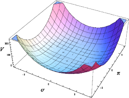
Figure 1: Form of the potential for $m_{0}^{2}>0$. A single minimum located in the origin is present.

In fact, along the $\sigma$-direction:

$$\partial_{\sigma}V(\sigma,0)=m_{0}^{2}\sigma+\lambda\sigma^{3}=0\text{ , }$$ (81)

out of which

$$\sigma=0\text{ and }\sigma=\pm\sqrt{\frac{-m_{0}^{2}}{\lambda}}\text{ .}$$ (82)

For $m_{0}^{2}>0$ the value $\sigma=0$ is the only solution. The masses of the particles corresponds to the second derivatives evaluated at the minimum:

$$m_{\pi}^{2} =\left.\frac{\partial^{2}V}{\partial\pi^{2}}\right|_{P=P_{\min}}=m_{0}^{2}\text{ ,}$$ (83)

$$m_{\sigma}^{2} =\left.\frac{\partial^{2}V}{\partial\sigma^{2}}\right|_{P=P_{\min}}=m_{0}^{2}\text{ .}$$ (84)

As expected, both particles have the same mass $m_{0}.$ This is a direct consequence of chiral symmetry.

We know however that Nature is not like that. The pion is nearly massless ($\simeq 135$ MeV) but the sigma field, which shall be identified with $f_{0}(1370),$ is much heavier: $1350\pm 150$ MeV. The reason for that is the spontaneous symmetry breaking. We can describe it in our model by considering

$$m_{0}^{2}<0\text{ . }$$ (85)

(Then, $m_{0}$ is purely imaginary). The corresponding potential can be rewritten as:

$$V(\sigma,\pi)=\frac{\lambda}{4}\left(\pi^{2}+\sigma^{2}-F^{2}\right)^{2}+const\text{ .}$$ (86)

It has the typical shape of a Mexican hat, in which the origin is not a minimum but a maximum, see Fig. 2.

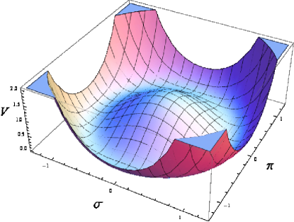
Figure 2: Form of the potential for $m_{0}^{2}<0$. A circle of minima is present.

The origin is not stable. In fact, upon calculating the masses around the origin, they would turn out to be imaginary. There is however a circle of equivalent minima for:

$$\pi^{2}+\sigma^{2}=-\frac{m_{0}^{2}}{\lambda}>0\text{ .}$$ (87)

According to spontaneous symmetry breaking, only one of them is realized. Clearly we cannot predict which one. We choose (they are all equivalent):

$$P_{\min}=\left(F=\sqrt{-\frac{m_{0}^{2}}{\lambda}},0\right)\text{ .}$$ (88)

After having made this choice, the system has undergone spontaneous chiral symmetry breaking. The value of the $\sigma$-field at the minimum is given by:

$$\sigma_{\min}=\phi_{N}=\sqrt{-\frac{m_{0}^{2}}{\lambda}}=F\text{ .}$$ (89)

$\phi_{N}$ is also denoted as the chiral condensate and is indeed proportional to $\left\langle 0_{QCD}\left|\bar{q}q\right|0_{QCD}\right\rangle\neq 0.$

We now calculate the masses:

$$m_{\pi}^{2} =\left.\frac{\partial^{2}V}{\partial\pi^{2}}\right|_{P=P_{\min}}=0\text{ ,}$$ (90)

$$m_{\sigma}^{2} =\left.\frac{\partial^{2}V}{\partial\sigma^{2}}\right|_{P=P_{\min}}=m_{0}^{2}+3\lambda\phi_{N}^{2}=-2m_{0}^{2}=2\lambda\phi_{N}^{2}>0\text{ ,}$$ (91)

which are now very different from each other: the pion is massless as a consequence of the Goldstone theorem. On the contrary, the mass of the $\sigma$ is nonzero. One then realizes how spontaneous chiral symmetry breaking generates different masses for chiral partners. Note, $m_{\sigma}$ is proportional to the chiral condensate $\phi_{N}.$

In Nature, the pion is not exactly masses. In order to describe this fact, we modify the potential as

$$V(\sigma,\pi)=\frac{m_{0}^{2}}{2}\left(\pi^{2}+\sigma^{2}\right)+\frac{\lambda}{4}\left(\pi^{2}+\sigma^{2}\right)^{2}-h\sigma\text{ ,}$$ (92)

where $-h\sigma$ breaks chiral symmetry explicitly. This term follows directly from the mass term $-m\bar{q}q$ in the QCD Lagrangian. We thus expect that $h\propto m,$ where $m$ is the bare quark mass (for instance, the $u$ quark or the average $(m_{u}+m_{d})/2$). The form of the potential is depicted in Fig. 3.

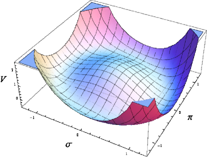
Figure 3: Form of the potential in presence of explicit symmetry breaking.

Now, it has a unique minimum along the $\sigma$ direction. The corresponding equation for $\phi_{N}$ reads:

$$\left.\frac{\partial V(\sigma,0)}{\partial\sigma}\right|_{\sigma=\sigma_{\min}=\phi_{N}} =m_{0}^{2}\phi_{N}+\lambda\phi_{N}^{3}-h\text{ }$$

$$=\phi_{N}\left(m_{0}^{2}+\lambda\phi_{N}^{2}\right)-h=0\text{ ,}$$ (93)

which is of third order. Only one of the three equation is physical, see Ref. [38]. The minimum is denoted as $P_{\min}=(\phi_{N},0).$ The pion mass is now nonzero:

$$m_{\pi}^{2}=\left.\frac{\partial^{2}V}{\partial\pi^{2}}\right|_{P=P_{\min}}=m_{0}^{2}+\lambda\phi_{N}^{2}=\frac{h}{\phi_{N}}>0\text{ .}$$ (94)

We realize that the pion mass scale as $m_{\pi}\propto\sqrt{h}\propto\sqrt{m}.$ This nontrivial dependence is a signature of an explicit symmetry breaking on top of a spontaneous symmetry breaking. For $h\rightarrow 0$ the pion mass vanishes, as expected.

The mass of the $\sigma$-particle is:

$$m_{\sigma}^{2}=\left.\frac{\partial^{2}V}{\partial\sigma^{2}}\right|_{P=P_{\min}}=m_{0}^{2}+3\lambda\phi_{N}^{2}=m_{\pi}^{2}+2\lambda\phi_{N}^{2}\text{ .}$$ (95)

Again, the mass of the $\sigma$-particle is always larger than the pion mass, The difference $m_{\sigma}^{2}-m_{\pi}^{2}=2\lambda\phi_{N}^{2}>0$ is not explicitly dependent on $h.$

The chiral condensate $\phi_{N}$ affects the masses and also decays, such as $\sigma\rightarrow\pi\pi$. The latter is determined in the following way: one first performs the shift $\sigma\rightarrow\sigma+\phi_{N}$ and then expands the potential. The term causing the decay is given by $\lambda\phi_{N}\sigma\pi^{2}.$ Hence:

$$\Gamma_{\sigma\rightarrow\pi^{2}}=s\frac{\left|\vec{k}\right|}{8\pi m_{\sigma}^{2}}\left[\lambda\phi_{N}\right]^{2}\text{ ,}$$ (96)

where $\left|\vec{k}\right|=\sqrt{\frac{m_{\sigma}^{2}}{4}-m_{\pi}^{2}}$ is the modulus of the three-momentum of one of the outgoing particles, and $s$ is a symmetry and isospin factor ($s=2$ in the present version of the model with only one type of pion, but $s=6$ when three pions are taken into account).

One can also show that $\phi_{N}$ enters into the expressions of the weak decay of pions. In the present version of the model, the condensate corresponds to the pion-decay constant: $\phi_{N}=f_{\pi}=92.4$ MeV [39].

In the full $N_{f}=3$ version of the model, the masses and decays are calculated by following the very same steps. Obviously, there are much more fields and decay channels, but the principle and the basic ideas are exactly the same as those discussed here.

3.2.4 A criterion for the construction of an hadronic model

We now come back to the Lagrangian of Eq. (78). One may wonder why terms of the type $(Tr[\Phi^{+}\Phi])^{6},$ which are also chirally symmetric, were not included. The fact that such a term would break renormalization is not a good argument: an effective hadronic theory is valid only in the low-energy sector and does not need to be renormalizable.

In order to understand this point, we need to introduce the dilaton field $G$. The corresponding Lagrangian has the general form:

$$\mathcal{L}_{G\Phi}=\frac{1}{2}(\partial_{\mu}G)^{2}-V_{dil}(G)+\mathrm{Tr}\left[(\partial^{\mu}\Phi)^{\dagger}(\partial^{\mu}\Phi)\right]-V_{G\Phi}\mathcal{(}G,\Phi)\text{ ,}$$ (97)

where $V_{dil}(G)=\frac{1}{4}\frac{m_{G}^{2}}{\Lambda_{G}^{2}}\left[G^{4}\ln\left(\frac{G}{\Lambda_{G}}\right)-\frac{G^{4}}{4}\right]$ was introduced in Eq. (66). Now, we require the two following properties:

(1) In the chiral limit $(m_{i}=0)$ there is in $\mathcal{L}_{G\Phi}$ a single dimensional parameter: the scale $\Lambda_{G}$ entering in the potential $V_{dil}(G)$. In this way the trace-anomaly is generated in the YM sector, in accordance with QCD.

(2) The potential $V_{G\Phi}\mathcal{(}G,\Phi)$ is finite when the fields are finite (smoothness of the potential).

These two criteria severely constrain the form of $\mathcal{L}_{G\Phi}.\$In fact, a term of the type

$$\alpha(\mathrm{Tr}[\Phi^{\dagger}\Phi])^{6}\text{ ,}$$ (98)

is not allowed because of (1) (the parameter $\alpha$ has dimension Energy^-2). One could still modify the term as

$$\frac{\beta}{G^{2}}(\mathrm{Tr}[\Phi^{\dagger}\Phi])^{6}$$ (99)

in which the constant $\beta$ is dimensionless and thus in agreement with (1). But point (2) is broken, since this term is singular for $G=0$. The validity of point (2) assures also that there is a smooth limit at high temperatures in which the gluon condensate $G_{0}$ is expected to become small.

As a consequence of (1) and (2), one has to consider only interaction terms with dimension exactly equal to four:

$$\mathcal{L}_{G\Phi} =\frac{1}{2}(\partial_{\mu}G)^{2}-V_{dil}(G)$$

$$+\mathrm{Tr}\left[(\partial^{\mu}\Phi)^{\dagger}(\partial_{\mu}\Phi)-aG^{2}\Phi^{\dagger}\Phi-\lambda_{2}\left(\Phi^{\dagger}\Phi\right)^{2}\right]-\lambda_{1}(\mathrm{Tr}[\Phi^{\dagger}\Phi])^{2}\text{ .}$$ (100)

The term $aG^{2}\Phi^{+}\Phi$ describes the interaction of the glueball and (pseudo)scalar mesons. The connection to $\mathcal{L}_{\Phi}$ of Eq. (78) is clear:

$$m_{0}^{2}=aG_{0}^{2}\text{ ,}$$ (101)

where $a$ is dimensionless. (In presence of quarkonia $G_{0}\simeq$ $\Lambda_{G}$ but is not exactly equal because mixing arises.) In conclusion, it is not renormalization but scale invariance (broken solely by $\Lambda_{G})$ which obliges us to take into account terms with dimension exactly equal to 4.

The large-$N_{c}$ dependence of the parameters reads:

$$a \propto N_{c}^{-2}\rightarrow m_{0}^{2}\propto N_{c}^{0}\text{ ,}$$ (102)

$$\lambda_{2} \propto N_{c}^{-1}\text{ ,}$$ (103)

$$\lambda_{1} \propto N_{c}^{-2}\text{ .}$$ (104)

The $\lambda_{2}$-term scales as $N_{c}^{-1}$ in agreement with Section 2.3. However, $\lambda_{1}$ scales as $N_{c}^{-2}$ because it arises as the product of two traces. One can have transitions in which all quark lines are annihilated, what implies an additional suppression of $N_{c}.$

3.2.5 Spontaneous symmetry breaking revisited

We already described spontaneous symmetry breaking in Sec. 3.2.3. In the present section, we reconsider it in the presence of $G.$ Upon setting $\Phi=\sigma t^{0}$ the potential reads:

$$V(G,\sigma)=V_{dil}(G)+aG^{2}\sigma^{2}+(\lambda_{2}+\lambda_{1})\sigma^{4}\text{.}$$ (105)

Then:

$\bullet$ $a>0\rightarrow$ $m_{0}^{2}=aG_{0}^{2}>0.$ Minimum for $G_{0}\neq 0,$ $\sigma_{0}=0$,

$\bullet$ $a<0\rightarrow$ $m_{0}^{2}=aG_{0}^{2}<0.$ Minimum for $G_{0}\neq 0,$ $\sigma_{0}\neq 0.$

Then, for $a<0,$ spontaneous breaking of chiral symmetry is realized for

$$\sigma_{0}\sim\sqrt{-\frac{m_{0}^{2}}{\lambda_{1}+\lambda_{2}}}\sim\sqrt{-\frac{a}{\lambda_{1}+\lambda_{2}}}G_{0}\text{ .}$$ (106)

Being $G_{0}\sim\Lambda_{G},$ it follows that $\sigma_{0}\propto\Lambda_{G}.$ Thus, the chiral condensate is also a consequence of the breaking of dilatation symmetry. Indeed, the trace anomaly is a very fundamental property of QCD which is at the basis of all low-energy hadronic phenomena.

3.2.6 $U(1)_{A}$ anomaly

The $U(1)_{A}$ anomaly is taken into account by the following additional term:

$$\mathcal{L}_{U(1)_{A}}=c_{1}(\det\Phi^{\dagger}-\det\Phi)^{2}\text{ .}$$ (107)

This term is invariant under $SU(N_{f})_{R}\times SU(N_{f})_{L}$. In fact, using $\det[ABC]=\det[A]\det[B]\det[C]$ one can see that $\Phi\rightarrow U_{L}\Phi U_{R}^{\dagger}$ does not change $\mathcal{L}_{U(1)_{A}}.$ This term is however not invariant under $U(1)_{A}$, for which $\Phi\rightarrow e^{2i\nu t^{0}}\Phi.$ In fact:

$$\mathcal{L}_{U(1)_{A}} =c_{1}\left(\det\Phi^{{\dagger}}-\det\Phi\right)^{2}$$

$$\rightarrow c_{1}\left(e^{-i\nu\sqrt{2N_{f}}}\det\Phi^{{\dagger}}-e^{i\nu\sqrt{2N_{f}}}\det\Phi\right)^{2}\neq\mathcal{L}_{U(1)_{A}}\text{ .}$$ (108)

This term influence the masses of the (pseudo)scalar mesons and is responsible for the large mass of $\eta^{\prime}$ ($\sim$ 1 GeV).

3.2.7 Vector and Axial-vector mesons

Vector and axial-vector mesons are light ($\lesssim 1.4$ GeV) and must be included in a realistic mesonic model of QCD. A general description of the issue was already presented in Ref. [40]. In Refs. [9, 41, 42] chiral models for $N_{f}=2$ were explicitly constructed. Yet, the full $N_{f}=3$ case was constructed only very recently in Ref. [11].

We now repeat the previous steps for (axial-)vector states. Mathematically, one introduces $N_{f}\times N_{f}$ matrices $R_{\mu}$ and $L_{\mu}:$

$$R_{ij}^{\mu}\equiv\sqrt{2}\overline{q}_{j,R}\gamma^{\mu}\overline{q}_{i,R}=\frac{1}{\sqrt{2}}\left(\overline{q}_{j}\gamma^{\mu}\overline{q}_{i}-\overline{q}_{j}\gamma^{5}\gamma^{\mu}\overline{q}_{i}\right)\text{ ,}$$ (109)

$$L_{ij}^{\mu}\equiv\sqrt{2}\overline{q}_{j,R}\gamma^{\mu}\overline{q}_{i,R}=\frac{1}{\sqrt{2}}\left(\overline{q}_{j}\gamma^{\mu}\overline{q}_{i}+\overline{q}_{j}\gamma^{5}\gamma^{\mu}\overline{q}_{i}\right)\text{ .}$$ (110)

Under chiral transformations they transform as:

$$R^{\mu}\rightarrow U_{R}R^{\mu}U_{R}^{\dagger}\text{ , }L^{\mu}\rightarrow U_{L}L^{\mu}U_{L}^{\dagger}\text{ .}$$ (111)

The matrices $R_{\mu}$ and $L_{\mu}$ are linear combinations of the vector and axial-vector fields $V_{\mu}$ and $A_{\mu}$

$$R^{\mu}=V^{\mu}-A^{\mu}\text{ },$$ (112)

$$L^{\mu}=V^{\mu}+A^{\mu}\text{ ,}$$ (113)

with:

$$V_{ij}^{\mu} \equiv\frac{1}{\sqrt{2}}\overline{q}_{j}\gamma^{\mu}\overline{q}_{i}=V^{\mu,a}t^{a}\text{ };V^{\mu,a}\equiv\sqrt{2}\overline{q}\gamma^{\mu}t^{a}q\text{ ,}$$ (114)

$$\text{ }A_{ij}^{\mu} \equiv\frac{1}{\sqrt{2}}\overline{q}_{j}\gamma^{5}\gamma^{\mu}\overline{q}_{i}=A^{\mu,a}t^{a}\text{ };A^{\mu,a}\equiv\sqrt{2}\overline{q}\gamma^{5}\gamma^{\mu}t^{a}q\text{ .}$$ (115)

Tables 2 and 3 show the transformations of $R^{\mu},L^{\mu}$ and $V_{\mu}$, $A_{\mu}.$

Table 2: Transformations of $R_{\mu}$ and $L_{\mu}$ [16]

	$R_{\mu}$	$L_{\mu}$
Elements	$R_{ij}^{\mu}\equiv\sqrt{2}\overline{q}_{j,R}\gamma^{\mu}q_{i,R}$	$L_{ij}^{\mu}\equiv\sqrt{2}\overline{q}_{j,R}\gamma^{\mu}q_{i,R}$
Currents	$R_{\mu}^{i}\equiv\overline{q}_{R}\gamma^{\mu}\frac{\lambda_{i}}{\sqrt{2}}q_{R}$	$L_{\mu}^{i}\equiv\overline{q}_{L}\gamma^{\mu}\frac{\lambda_{i}}{\sqrt{2}}q_{L}$
$P$	$g^{\mu\nu}L_{\mu}\mathcal{(}x^{0},-\mathbf{x}\mathcal{)}$	$g^{\mu\nu}R_{\mu}\mathcal{(}x^{0},-\mathbf{x}\mathcal{)}$
$C$	$-L_{\mu}^{t}$	$R_{\mu}^{t}$
$U(N_{f})_{V}$	$U_{V}R_{\mu}U_{V}^{\dagger}$	$U_{V}L_{\mu}U_{V}^{\dagger}$
$U(N_{f})_{A}$	$U_{A}R_{\mu}U_{A}^{\dagger}$	$U_{A}^{\dagger}L_{\mu}U_{A}$
$U(N_{f})_{R}\times$ $U(N_{f})_{L}$	$U_{R}R_{\mu}U_{R}^{\dagger}$	$U_{L}R_{\mu}U_{L}^{\dagger}$

Table 3: Transformations of $V_{\mu}$ and $A_{\mu}$ [16]

	$V_{\mu}$	$A_{\mu}$
Elements	$V_{ij}^{\mu}\equiv\sqrt{2}\overline{q}_{j}\gamma^{\mu}q_{i}$	$A_{ij}^{\mu}\equiv\sqrt{2}\overline{q}_{j}\gamma^{5}\gamma^{\mu}q_{i}$
Currents	$V^{i}\equiv\overline{q}\gamma^{\mu}\frac{\lambda_{i}}{\sqrt{2}}q$	$A^{i}\equiv\overline{q}\gamma^{5}\gamma^{\mu}\frac{\lambda_{i}}{\sqrt{2}}q$
$P$	$g^{\mu\nu}V_{\mu}\mathcal{(}x^{0},-\mathbf{x}\mathcal{)}$	$-g^{\mu\nu}A_{\mu}\mathcal{(}x^{0},-\mathbf{x}\mathcal{)}$
$C$	$-V_{\mu}^{t}$	$A_{\mu}^{t}$

Notice that under parity a vector-field, such as the $\rho$-meson, transforms as $\rho^{i}(t,\mathbf{x})\rightarrow-\rho^{i}(t,-\mathbf{x})$, $\rho^{0}(t,\mathbf{x})\rightarrow\rho^{0}(t,-\mathbf{x})$. This is why at nonzero density the field $\omega^{0}$ and $\rho^{0}$ (may) condense.

The corresponding Lagrangian $\mathcal{L}_{AV}$ is constructed by following the very same principles of Sec. 3.2.1 and 3.2.4. It consists of the sum

$$\mathcal{L}_{AV}=\mathcal{L}_{2,AV}+\mathcal{L}_{3,AV}+\mathcal{L}_{4,AV}+\mathcal{L}_{PS,AV}\text{ ,}$$ (116)

where 2, 3, 4 is the number of (axial-)vector fields at each vertex and where $\mathcal{L}_{\Phi,AV}$ describes the interaction with (pseudo)scalar quarkonium states.

The term $\mathcal{L}_{2,AV}$ reads

$$\mathcal{L}_{2,AV}=-\frac{1}{4}\mathrm{Tr}[(L^{\mu\nu})^{2}+(R^{\mu\nu})^{2}]+\frac{b}{2}G^{2}\mathrm{Tr}[(L^{\mu})^{2}+(R^{\mu})^{2}]\text{ ,}$$ (117)

$$L^{\mu\nu}=\partial^{\mu}L^{\nu}-\partial^{\nu}L^{\mu},\text{ }R^{\mu\nu}=\partial^{\mu}R^{\nu}-\partial^{\nu}R^{\mu}\text{ .}$$ (118)

When the dilaton condense a mass-term for the (axial-)vector d.o.f. arises:

$$m_{1}^{2}=bG_{0}^{2}\text{ .}$$ (119)

$\mathcal{L}_{3,AV}$ and $\mathcal{L}_{4,AV}$ are:

$$\mathcal{L}_{3,AV}=-2ig_{2}\left(\mathrm{Tr}[L_{\mu\nu}[L^{\mu},L^{\nu}]]+\mathrm{Tr}[R_{\mu\nu}[R^{\mu},R^{\nu}]]\right)\text{ ,}$$ (120)

$$\mathcal{L}_{4,AV} =g_{3}\left\{\mathrm{Tr}\left[L^{\mu}L^{\nu}L_{\mu}L_{\nu}\right]+\mathrm{Tr}\left[R^{\mu}R^{\nu}R_{\mu}R_{\nu}\right]\right\}+$$

$$g_{4}\left\{\mathrm{Tr}\left[L^{\mu}L_{\mu}L^{\nu}L_{\nu}\right]+\mathrm{Tr}\left[R^{\mu}R_{\mu}R^{\nu}R_{\nu}\right]\right\}$$

$$g_{5}\mathrm{Tr}\left[R^{\mu}R_{\mu}\right]\mathrm{Tr}\left[L^{\mu}L_{\mu}\right]+$$

$$g_{6}\left\{\mathrm{Tr}[L_{\mu}L^{\mu}]\mathrm{Tr}[L_{\mu}L^{\mu}]+\mathrm{Tr}[R_{\mu}R^{\mu}]\mathrm{Tr}[R_{\mu}R^{\mu}]\right\}\text{ .}$$ (121)

$\mathcal{L}_{4,AV}$ does not influence decays and is not relevant here. Finally:

$$\mathcal{L}_{\Phi,AV} =\mathrm{Tr}\left[(ig_{1}(\Phi R^{\mu}-L^{\mu}\Phi))^{\dagger}(\partial^{\mu}\Phi)\right]+\mathrm{Tr}\left[(\partial^{\mu}\Phi)^{\dagger}(ig_{1}(\Phi R^{\mu}-L^{\mu}\Phi))\right]$$

$$+\mathrm{Tr}\left[(ig_{1}(\Phi R^{\mu}-L^{\mu}\Phi))^{\dagger}(ig_{1}(\Phi R^{\mu}-L^{\mu}\Phi))\right]$$

$$+\frac{h_{1}}{2}\mathrm{Tr}\left[\Phi\Phi^{{\dagger}}\right]Tr\left[L_{\mu}L^{\mu}+R_{\mu}R^{\mu}\right]$$

$$+h_{2}\mathrm{Tr}\left[\Phi^{{\dagger}}L_{\mu}L^{\mu}\Phi+\Phi R_{\mu}R^{\mu}\Phi\right]+2h_{3}\mathrm{Tr}\left[\Phi R_{\mu}\Phi^{{\dagger}}L^{\mu}\right]\text{ }.$$ (122)

The large-$N_{c}$ dependence of the parameters is:

$$g_{1},\text{ }g_{2},\text{ }g \propto N_{c}^{-1/2}\;,$$

$$\text{ }h_{2},\text{ }h_{3},\text{ }g_{3},\text{ }g_{4} \propto N_{c}^{-1}\;,$$

$$\text{ }h_{1},\text{ }g_{5},\text{ }g_{6} \propto N_{c}^{-2}\;,$$

$$b\propto N_{c}^{-2}\rightarrow m_{1}^{2}\propto N_{c}^{0}\;.$$ (123)

3.2.8 Explicit breaking of chiral symmetry through bare quark masses

The nonzero quark masses is taken into account by the term:

$$\mathrm{Tr}[H(\Phi^{{\dagger}}+\Phi)]\text{ ,}$$ (124)

$$H=diag\{h_{0}^{1},h_{0}^{2},...,h_{0}^{N_{f}}\}$$ (125)

with $h_{0}^{k}\propto m_{k}$ and $h_{0}^{k}\propto N_{c}^{1/2}$. The effect of this object was already studied in Sec. 3.2.3. A unique minimum of the potential exists.

Further chiral breaking terms are given by

$$\mathrm{Tr}[\varepsilon\Phi^{{\dagger}}\Phi]\text{ ,}$$ (126)

$$\frac{1}{2}\mathrm{Tr}[\delta(L^{\mu})^{2}+(R^{\mu})^{2}]\text{ ,}$$ (127)

where $\varepsilon$ and $\delta$ are diagonal matrices whose $k$-element is proportional to $m_{k}^{2}.$ These terms generate a standard contribution to the meson masses. Indeed, when $\varepsilon$ and $\delta$ are proportional to the identity, these terms can be absorbed away and have no influence on the results. It is then the difference of masses which is important here.

Finally the explicit symmetry breaking Lagrangian is given by

$$\mathcal{L}_{eSB}=\mathrm{Tr}[H(\Phi^{{\dagger}}+\Phi)]+\mathrm{Tr}[\varepsilon\Phi^{{\dagger}}\Phi]+\frac{1}{2}\mathrm{Tr}[\delta(L^{\mu})^{2}+(R^{\mu})^{2}]\text{ .}$$ (128)

3.2.9 The whole Lagrangian of the eLSM

We now put all the elements together and finally obtain the Lagrangian of the extended Linear Sigma Model in the mesonic sector:

$$\mathcal{L}_{eLSM}=\mathcal{L}_{G\Phi}+\mathcal{L}_{AV}+\mathcal{L}_{U_{A}(1)}+\mathcal{L}_{eSB}\text{ .}$$ (129)

Explicitly:

$$\mathcal{L}_{eLSM} =\frac{1}{2}(\partial_{\mu}G)^{2}-\frac{1}{4}\frac{m_{G}^{2}}{\Lambda_{G}^{2}}\left[G^{4}\ln\left(\frac{G}{\Lambda_{G}}\right)-\frac{G^{4}}{4}\right]$$

$$+\mathrm{Tr}\left[(D^{\mu}\Phi)^{\dagger}(D_{\mu}\Phi)-aG^{2}\Phi^{{\dagger}}\Phi-\lambda_{2}\left(\Phi^{{\dagger}}\Phi\right)^{2}\right]-\lambda_{1}(\mathrm{Tr}[\Phi^{{\dagger}}\Phi])^{2}$$

$$+c_{1}(\det\Phi^{{\dagger}}-\det\Phi)^{2}\text{ }+\mathrm{Tr}[H(\Phi^{{\dagger}}+\Phi)]+\mathrm{Tr}[\varepsilon\Phi^{{\dagger}}\Phi]+\text{.}$$

$$-\frac{1}{4}\mathrm{Tr}[(L^{\mu\nu})^{2}+(R^{\mu\nu})^{2}]+\frac{b}{2}G^{2}\mathrm{Tr}[(L^{\mu})^{2}+(R^{\mu})^{2}]$$

$$+\frac{1}{2}\mathrm{Tr}[\delta(L^{\mu})^{2}+(R^{\mu})^{2}]\text{ }$$

$$-2ig_{2}\left(\mathrm{Tr}[L_{\mu\nu}[L^{\mu},L^{\nu}]]+\mathrm{Tr}[R_{\mu\nu}[R^{\mu},R^{\nu}]]\right)$$

$$+\frac{h_{1}}{2}\mathrm{Tr}\left[\Phi\Phi^{{\dagger}}\right]Tr\left[L_{\mu}L^{\mu}+R_{\mu}R^{\mu}\right]+$$

$$+h_{2}\mathrm{Tr}\left[\Phi^{{\dagger}}L_{\mu}L^{\mu}\Phi+\Phi R_{\mu}R^{\mu}\Phi\right]+2h_{3}\mathrm{Tr}\left[\Phi R_{\mu}\Phi^{{\dagger}}L^{\mu}\right]\text{ }+...\text{,}$$ (130)

with

$$D^{\mu}\Phi=\partial^{\mu}\Phi-ig_{1}(L^{\mu}\Phi-\Phi R^{\mu})\text{ .}$$ (131)

This is a realistic model of low-energy QCD which includes from the very beginning (pseudo)scalar and (axial-)vector quarkonia and one scalar glueball. Next, we show the comparison with data.

3.3 Results for the case $N_{f}=3$

In Ref. [11] the case $N_{f}=3$ has been studied in detail. In the first step, the glueball $G$ is frozen: we simply set $G=G_{0}$ and do not consider its fluctuations (this is done later on). In Table 4 we show the assignments of the fields entering in model and their PDG counterparts.

Table 4: Fields and correspondence to PDG

Field	PDG	Quark content	$I$	$J^{PC}$	Mass (MeV)
$\pi^{+},\pi^{-},\pi^{0}$	$\pi$	$u\bar{d},d\bar{u},\frac{u\bar{u}-d\bar{d}}{\sqrt{2}}$	$1$	$0^{-+}$	$139.57$
$K^{+},K^{-},K^{0},\bar{K}^{0}$	$K$	$u\bar{s},s\bar{u},d\bar{s},s\bar{d}$	$1/2$	$0^{-+}$	$493.677$
$\eta_{N}a+\eta_{S}b$	$\eta$	$\frac{u\bar{u}+d\bar{d}}{\sqrt{2}}a+s\bar{s}b$	$0$	$0^{-+}$	$547.86$
$-\eta_{N}a+\eta_{S}b$	$\eta^{\prime}(958)$	$\frac{u\bar{u}+d\bar{d}}{\sqrt{2}}a+s\bar{s}b$	$0$	$0^{-+}$	$957.78$
$a_{0}^{+},a_{0}^{-},a_{0}^{0}$	$a_{0}(1450)$	$u\bar{d},d\bar{u},\frac{u\bar{u}-d\bar{d}}{\sqrt{2}}$	$1$	$0^{++}$	$1474$
$K_{S}^{+},K_{S}^{-},K_{S}^{0},\bar{K}_{S}^{0}$	$K_{0}^{\ast}(1430)$	$u\bar{s},s\bar{u},d\bar{s},s\bar{d}$	$1/2$	$0^{++}$	$1425$
$\sigma_{N}$	$f_{0}(1370)$	$\frac{u\bar{u}+d\bar{d}}{\sqrt{2}}$	$0$	$0^{++}$	$1350$
$\sigma_{S}$	$f_{0}(1500)$	$s\bar{s}$	$0$	$0^{++}$	$1504$
$\rho^{+},\rho^{-},\rho^{0}$	$\rho(770)$	$u\bar{d},d\bar{u},\frac{u\bar{u}-d\bar{d}}{\sqrt{2}}$	$1$	$1^{--}$	$775.26$
$K^{\ast+},K^{\ast-},K^{\ast 0},\bar{K}^{\ast 0}$	$K^{\ast}(892)$	$u\bar{s},s\bar{u},d\bar{s},s\bar{d}$	$1/2$	$1^{--}$	$891.86$
$\omega_{N}$	$\omega(782)$	$\frac{u\bar{u}+d\bar{d}}{\sqrt{2}}$	$0$	$1^{--}$	$782.65$
$\omega_{S}$	$\phi(1020)$	$s\bar{s}$	$0$	$1^{--}$	$1019.461$
$a_{1}^{+},a_{1}^{-},a_{1}^{0}$	$a_{1}(1230)$	$u\bar{d},d\bar{u},\frac{u\bar{u}-d\bar{d}}{\sqrt{2}}$	$1$	$1^{++}$	$1230$
$K_{1}^{+},K_{1}^{-},K_{1}^{0},\bar{K}_{1}^{0}$	$K_{1}(1270)$	$u\bar{s},s\bar{u},d\bar{s},s\bar{d}$	$1/2$	$1^{++}$	$1272$
$f_{1,N}$	$f_{1}(1285)$	$\frac{u\bar{u}+d\bar{d}}{\sqrt{2}}$	$0$	$1^{++}$	$1281.9$
$f_{1,S}$	$f_{1}(1420)$	$s\bar{s}$	$0$	$1^{++}$	$1426.4$

The masses of the particles were calculated in Refs. [11, 38]. The procedure is the same of Sec. 3.2.3, just a bit longer because many fields are present.

The pseudoscalar masses are:

$$m_{\pi}^{2} =Z_{\pi}^{2}\left[m_{0}^{2}+\left(\lambda_{1}+\frac{\lambda_{2}}{2}\right)\phi_{N}^{2}+\lambda_{1}\phi_{S}^{2}\right]\equiv\frac{Z_{\pi}^{2}h_{0N}}{\phi_{N}}\text{ ,}$$ (132)

$$m_{K}^{2} =Z_{K}^{2}\left[m_{0}^{2}+\left(\lambda_{1}+\frac{\lambda_{2}}{2}\right)\phi_{N}^{2}-\frac{\lambda_{2}}{\sqrt{2}}\phi_{N}\phi_{S}+\left(\lambda_{1}+\lambda_{2}\right)\phi_{S}^{2}\right]\text{ ,}$$ (133)

$$m_{\eta_{N}}^{2} =Z_{\pi}^{2}\left[m_{0}^{2}+\left(\lambda_{1}+\frac{\lambda_{2}}{2}\right)\phi_{N}^{2}+\lambda_{1}\phi_{S}^{2}+c_{1}\,\phi_{N}^{2}\phi_{S}^{2}\right]$$

$$\equiv Z_{\pi}^{2}\left(\frac{h_{0N}}{\phi_{N}}+c_{1}\,\phi_{N}^{2}\phi_{S}^{2}\right)\;,$$ (134)

$$m_{\eta_{S}}^{2} =Z_{\eta_{S}}^{2}\left[m_{0}^{2}+\lambda_{1}\phi_{N}^{2}+\left(\lambda_{1}+\lambda_{2}\right)\phi_{S}^{2}+\frac{c_{1}}{4}\phi_{N}^{4}\right]$$

$$\equiv Z_{\eta_{S}}^{2}\left(\frac{h_{0S}}{\phi_{S}}+\frac{c_{1}}{4}\phi_{N}^{4}\right)\text{ ,}$$ (135)

$$m_{\eta_{NS}}^{2} =Z_{\pi}Z_{\pi_{S}}\frac{c_{1}}{2}\phi_{N}^{3}\phi_{S}\text{ ,}$$ (136)

where $m_{\eta_{NS}}^{2}$ is a mixing term, leading to:

$$\;m_{\eta^{\prime}/\eta}^{2}=\frac{1}{2}\left[m_{\eta_{N}}^{2}+m_{\eta_{S}}^{2}\pm\sqrt{(m_{\eta_{N}}^{2}-m_{\eta_{S}}^{2})^{2}+4m_{\eta_{NS}}^{4}}\right]\;.$$ (137)

The constants $Z_{k}$ arise when unphysical axial-vector-pseudoscalar mixing terms are eliminated by proper shifts and renormalization constants, see details in Ref. [11]. They read:

$$Z_{\pi} =Z_{\eta_{N}}=\frac{m_{a_{1}}}{\sqrt{m_{a_{1}}^{2}-g_{1}^{2}\phi_{N}^{2}}}\text{ ,} Z_{K} =\frac{2m_{K_{1}}}{\sqrt{4m_{K_{1}}^{2}-g_{1}^{2}(\phi_{N}+\sqrt{2}\phi_{S})^{2}}}\text{ ,}$$ (138)

$$Z_{\eta_{S}} =\frac{m_{f_{1S}}}{\sqrt{m_{f_{1S}}^{2}-2g_{1}^{2}\phi_{S}^{2}}}\text{ ,} Z_{K_{0}^{\star}} =\frac{2m_{K^{\star}}}{\sqrt{4m_{K^{\star}}^{2}-g_{1}^{2}(\phi_{N}-\sqrt{2}\phi_{S})^{2}}}\;.$$ (139)

The masses of the scalar mesons are:

$$m_{a_{0}}^{2} =m_{0}^{2}+\left(\lambda_{1}+\frac{3}{2}\lambda_{2}\right)\phi_{N}^{2}+\lambda_{1}\phi_{S}^{2}\text{ ,}$$ (140)

$$m_{K_{0}^{\star}}^{2} =Z_{K_{0}^{\star}}^{2}\left[m_{0}^{2}+\left(\lambda_{1}+\frac{\lambda_{2}}{2}\right)\phi_{N}^{2}+\frac{\lambda_{2}}{\sqrt{2}}\phi_{N}\phi_{S}+\left(\lambda_{1}+\lambda_{2}\right)\phi_{S}^{2}\right]\text{ ,}$$ (141)

$$m_{\sigma_{N}}^{2} =m_{0}^{2}+3\left(\lambda_{1}+\frac{\lambda_{2}}{2}\right)\phi_{N}^{2}+\lambda_{1}\phi_{S}^{2}\text{ ,}$$ (142)

$$m_{\sigma_{S}}^{2} =m_{0}^{2}+\lambda_{1}\phi_{N}^{2}+3\left(\lambda_{1}+\lambda_{2}\right)\phi_{S}^{2}\text{ .}$$ (143)

The masses of the vector mesons are:

$$m_{\rho}^{2} =m_{1}^{2}+\frac{1}{2}(h_{1}+h_{2}+h_{3})\phi_{N}^{2}+\frac{h_{1}}{2}\phi_{S}^{2}+2\delta_{N}\;,$$ (144)

$$m_{K^{\star}}^{2} =m_{1}^{2}+\frac{1}{4}\left(g_{1}^{2}+2h_{1}+h_{2}\right)\phi_{N}^{2}$$

$$+\frac{1}{\sqrt{2}}\phi_{N}\phi_{S}(h_{3}-g_{1}^{2})+\frac{1}{2}(g_{1}^{2}+h_{1}+h_{2})\phi_{S}^{2}+\delta_{N}+\delta_{S}\;,$$ (145)

$$m_{\omega_{N}}^{2} =m_{\rho}^{2}\;,$$ (146)

$$m_{\omega_{S}}^{2} =m_{1}^{2}+\frac{h_{1}}{2}\phi_{N}^{2}+\left(\frac{h_{1}}{2}+h_{2}+h_{3}\right)\phi_{S}^{2}+2\delta_{S}\;,$$ (147)

The masses of axial-vector mesons are:

$$m_{a_{1}}^{2} =m_{1}^{2}+\frac{1}{2}(2g_{1}^{2}+h_{1}+h_{2}-h_{3})\phi_{N}^{2}+\frac{h_{1}}{2}\phi_{S}^{2}+2\delta_{N}\;,$$ (148)

$$m_{K_{1}}^{2} =m_{1}^{2}+\frac{1}{4}\left(g_{1}^{2}+2h_{1}+h_{2}\right)\phi_{N}^{2}$$

$$-\frac{1}{\sqrt{2}}\phi_{N}\phi_{S}(h_{3}-g_{1}^{2})+\frac{1}{2}\left(g_{1}^{2}+h_{1}+h_{2}\right)\phi_{S}^{2}+\delta_{N}+\delta_{S}\;,$$ (149)

$$m_{f_{1N}}^{2} =m_{a_{1}}^{2}\;,$$ (150)

$$m_{f_{1S}}^{2} =m_{1}^{2}+\frac{h_{1}}{2}\phi_{N}^{2}+\left(2g_{1}^{2}+\frac{h_{1}}{2}+h_{2}-h_{3}\right)\phi_{S}^{2}+2\delta_{S}\;.$$ (151)

The potential depends on two condensates $\phi_{N}\equiv\left\langle\bar{u}u+\bar{d}d\right\rangle/\sqrt{2},$ $\phi_{S}\equiv\left\langle ss\right\rangle$, the light-quark condensate and the strange quark condensate, respectively (the discussion is still very similar to Sec. 3.2.3):

$$\mathcal{V}(\phi_{N},\phi_{S}) =\frac{1}{2}m_{0}^{2}(\phi_{N}^{2}+\phi_{S}^{2})+\frac{\lambda_{1}}{4}(\phi_{N}^{4}+2\phi_{N}^{2}\phi_{S}^{2}+\phi_{S}^{4})$$

$$+\frac{\lambda_{2}}{4}\left(\frac{\phi_{N}^{4}}{2}+\phi_{S}^{4}\right)-h_{0N}\phi_{N}-h_{0S}\phi_{S}\text{ .}$$ (152)

One obtains$\ \phi_{N}$ and $\phi_{S}\$upon minimization$:$

$$\frac{\partial\mathcal{V}(\phi_{N},\phi_{S})}{\partial\phi_{N}}\overset{!}{=}0 \Leftrightarrow h_{0N}=[m_{0}^{2}+\lambda_{1}(\phi_{N}^{2}+\phi_{S}^{2})]\phi_{N}+\frac{\lambda_{2}}{2}\phi_{N}^{3}\text{ ,}$$ (153)

$$\frac{\partial\mathcal{V}(\phi_{N},\phi_{S})}{\partial\phi_{S}}\overset{!}{=}0 \Leftrightarrow h_{0S}=[m_{0}^{2}+\lambda_{1}(\phi_{N}^{2}+\phi_{S}^{2})]\phi_{S}+\lambda_{2}\phi_{S}^{3}\text{ .}$$ (154)

In summary, the masses depend on the two chiral condensates. It is easy to see that particles come in chiral partners, which become degenerate when the condensates vanish. The situation is indeed in principle very similar to Sec. 3.2.3, although much more complicated from a technical point of view. The calculation of decays can be carried out in a straightforward way, which however requires some hard work [11, 38].

Table 5 : Values of the parameters (from [11]).

Parameter Value

$$m_{0}^{2}$$

             (155)

Table 6: Results of the fit (from [11])

Observable Fit $$\left[\text{MeV}\right]$$ Experiment

        

Eleven parameters, listed in Table 5, were fitted to 21 experimental quantities listed in Table 6. (Note: when the experimental error was smaller than 5% of the measured value, the error considered in the fit was set to 5%. This is because our model, which neglects in the present form isospin breaking, cannot achieve a higher precision).

Following considerations hold:

(i) The scalar quark-antiquark mesons lie above 1 GeV (see Table 6).

(ii) As a consequence of (i), the light scalar mesons with a mass below 1 GeV are something else (four-quark states, see the next section).

(iii) In Ref. [11] various consequences of the fit were investigated. For instance, the branching ratios of $a_{0}$ are in good agreement with the experimental data.

(iv) The spectral function of the $\rho$ and the $a_{1}$ meson can be successfully calculated [43].

(v) The eLSM has also been applied to baryons in the so-called mirror assignment [10].

(vi) Studies of the model at nonzero density have been performed in Refs. [44, 45].

(vii) Some preliminary attempts to study the eLSM at nonzero temperature have been undertaken in Refs. [46, 47].

(viii) The model has been successfully extended to the case $N_{f}=4$ [48], in which charmed mesons are included.

4 Glueballs in the eLSM

According to lattice QCD many glueballs with various quantum numbers should exist, see Ref. [32, 33, 49] and Table 7 (for the uncertainties, see Ref. [32]). However, up to now no glueball state has been unambiguously identified (although for some of them some candidates exist). The eSLM introduced in the previous section can help to elucidate some features of glueballs. In fact, the scalar glueball is a very important building block of the model and other glueballs, such as the pseudoscalar one, can be easily coupled to the eLSM.

Table 7: Central values of glueball masses from lattice (from [32]).

$J^{PC}$	Value [GeV]
$0^{++}$	$\,1.70$
$2^{++}$	$2.39$
$0^{-+}$	$2.55$
$1^{-+}$	$2.96$
$2^{-+}$	$3.04$
$3^{+-}$	$3.60$
$3^{++}$	$3.66$
$1^{--}$	$3.81$
$2^{--}$	$4.0$
$3^{--}$	$4.19$
$2^{+-}$	$4.22$
$0^{+-}$	$4.77$

4.1 Scalar glueball

The scalar glueball is the lightest gluonic state predicted by lattice QCD and is a natural element of the eLSM as the excitation of the dilaton field [11, 12]. The eLSM makes predictions for the lightest glueball state in a chiral framework, completing previous phenomenological works on the subject [50, 51, 52, 53]. The result of the recent study of Ref. [12] shows that the scalar glueball is predominately contained in the resonance $f_{0}(1710)$ This assignment is in agreement with the old lattice result of Ref. [54], with the recent lattice result of Ref. [55], with other hadronic approaches [51, 52] and lately also within an holographic approach [56].

The admixtures as calculated in Ref. [12] read:

$$\left(\begin{array}[c]{c}f_{0}(1370)\\ f_{0}(1500)\\ f_{0}(1710)\end{array}\right)=\left(\begin{array}[c]{ccc}-0.91&0.24&-0.33\\ 0.30&0.94&-0.17\\ -0.27&0.26&0.93\end{array}\right)\left(\begin{array}[c]{c}\sigma_{N}\\ \sigma_{S}\\ G\end{array}\right)\text{ }.$$ (156)

The following admixtures of the bare fields to the resonances follow:

$$f_{0}(1370): \quad 83\%\,\sigma_{N}\;,\quad 6\%\,\sigma_{S}\;,\quad 11\%\,G\text{ },$$

$$f_{0}(1500): \quad 9\%\,\sigma_{N}\;,\quad 88\%\,\sigma_{S}\;,\quad 3\%\,G\text{ },$$ (157)

$$f_{0}(1710): \quad 8\%\,\sigma_{N}\;,\quad 6\%\,\sigma_{S}\;,\quad 86\%\,G\text{ }.$$

The additional 5 parameters listed in Table 8 are needed in the scalar isoscalar sector. They were fitted to the experimental quantities of Table 9. Further predictions of the approach are reported in Table 10.

Table 8: Additional parameters for the $J^{PC}=0^{++}$ sector (from [12]).

Parameter	Value
$\Lambda$	$3297\,[$MeV$]$
$m_{G}$	$1525\,[$MeV$]$
$\lambda_{1}$	$6.25$
$h_{1}$	$-3.22$
$\epsilon_{S}$	$0.4212\times 10^{6}\,[$MeV${}^{2}]$

Table 9: Fitted quantities in the $J^{PC}=0^{++}$ sector (from [12]).

Quantity	Fit [MeV]	Exp. [MeV]
$M_{f_{0}(1370)}$	$1444$	$1200$-$1500$
$M_{f_{0}(1500)}$	$1534$	$1505\pm 6$
$M_{f_{0}(1710)}$	$1750$	$1720\pm 6$
$f_{0}(1370)\rightarrow\pi\pi$	$423.6$	-
$f_{0}(1500)\rightarrow\pi\pi$	$39.2$	$38.04\pm 4.95$
$f_{0}(1500)\rightarrow K\bar{K}$	$9.1$	$9.37\pm 1.69$
$f_{0}(1710)\rightarrow\pi\pi$	$28.3$	$29.3\pm 6.5$
$f_{0}(1710)\rightarrow K\bar{K}$	$73.4$	$71.4\pm 29.1$

In our solution, $f_{0}(1370)$ decays predominantly into two pions with a decay width of about $400$ MeV, in agreement with its interpretation as predominantly nonstrange $\bar{q}q$ state [11, 12]. This is in qualitative agreement with the experimental analysis of Ref. [57], where $\Gamma_{f_{0}(1370)\rightarrow\pi\pi}=325$ MeV, $\Gamma_{f_{0}(1370)\rightarrow 4\pi}\approx 50$ MeV, and $\Gamma_{f_{0}(1370)\rightarrow\eta\eta}/\Gamma_{f_{0}(1370)\rightarrow\pi\pi}=0.19\pm 0.07$. Moreover, the decay channel $f_{0}(1500)\rightarrow\eta\eta$ is in good agreement with PDG, while the decay channel $f_{0}(1710)\rightarrow\eta\eta$ is slightly larger than the experiment.

Table 10: further properties in the $J^{PC}=0^{++}$ sector (from [12]).

Decay Channel Our Value [MeV] Exp. [MeV] $f_{0}(1370)\rightarrow K\bar{K}$ $117.5$ - $f_{0}(1370)\rightarrow\eta\eta$ $43.3$ - $f_{0}(1370)\rightarrow\rho\rho\rightarrow 4\pi$ $13.8$ - $f_{0}(1500)\rightarrow\eta\eta$ $4.7$ $5.56\pm 1.34$ $f_{0}(1500)\rightarrow\rho\rho\rightarrow 4\pi$ $0.2$ $>54.0\pm 7.1$ $f_{0}(1710)\rightarrow\eta\eta$ $57.9$ $34.3\pm 17.6$ $f_{0}(1710)\rightarrow\rho\rho\rightarrow 4\pi$ $0.5$ -         

In conclusion, present results show that $f_{0}(1710)$ is a very good scalar glueball candidate.

4.2 The pseudoscalar glueball

The pseudoscalar glueball is related to the chiral anomaly and couples in a chirally invariant way to light mesons [13] and also to baryons [14]. The chiral Lagrangian which couples the pseudoscalar glueball $\tilde{G}\equiv\left|gg\right\rangle$ with quantum numbers $J^{PC}=0^{-+}$ to scalar and pseudoscalar mesons reads explicitly:

$$\mathcal{L}_{\tilde{G}}^{int}=ic_{\tilde{G}\Phi}\tilde{G}\left(\text{{det}}\Phi-\text{{det}}\Phi^{{\dagger}}\right)\text{ .}$$ (158)

The branching ratios of $\tilde{G}$ are reported in Table 11 for two choices of the pseudoscalar masses: $M_{\tilde{G}}=2.6$ GeV predicted by lattice QCD [32] and $M_{\tilde{G}}=2.37$ GeV, in agreement with the pseudoscalar particle $X(2370)$ measured by BES [58] (this resonance could be the pseudoscalar glueball). The branching ratios are presented relative to the total decay width of the pseudoscalar glueball $\Gamma_{\tilde{G}}^{tot}$.

Table 11: Branching ratios for the pseudoscalar glueball (from [13]).

Quantity	Case (i): $M_{\tilde{G}}=2.6$ GeV	Case (ii): $M_{\tilde{G}}=2.37$ GeV
$\Gamma_{\tilde{G}\rightarrow KK\eta}/\Gamma_{\tilde{G}}^{tot}$	$0.049$	$0.043$
$\Gamma_{\tilde{G}\rightarrow KK\eta^{\prime}}/\Gamma_{\tilde{G}}^{tot}$	$0.019$	$0.011$
$\Gamma_{\tilde{G}\rightarrow\eta\eta\eta}/\Gamma_{\tilde{G}}^{tot}$	$0.016$	$0.013$
$\Gamma_{\tilde{G}\rightarrow\eta\eta\eta^{\prime}}/\Gamma_{\tilde{G}}^{tot}$	$0.0017$	$0.00082$
$\Gamma_{\tilde{G}\rightarrow\eta\eta^{\prime}\eta^{\prime}}/\Gamma_{\tilde{G}}^{tot}$	$0.00013$	$0$
$\Gamma_{\tilde{G}\rightarrow KK\pi}/\Gamma_{\tilde{G}}^{tot}$	$0.47$	$0.47$
$\Gamma_{\tilde{G}\rightarrow\eta\pi\pi}/\Gamma_{\tilde{G}}^{tot}$	$0.16$	$0.17$
$\Gamma_{\tilde{G}\rightarrow\eta^{\prime}\pi\pi}/\Gamma_{\tilde{G}}^{tot}$	$0.095$	$0.090$

In conclusion, we predict that $KK\pi$ is the dominant decay channel (50%), followed by sizable $\eta\pi\pi$ and $\eta^{\prime}\pi\pi$ decay channels (16% and 10% respectively). Moreover, we also predict the decay into three pions should vanish:

$$\Gamma_{\tilde{G}\rightarrow\pi\pi\pi}=0\text{ .}$$ (159)

These are simple and testable theoretical predictions which can be helpful in the experimental search at the PANDA experiment [59], where the glueball can be directly formed in proton-antiproton fusion process.

4.3 Other glueballs

A similar program can be carried out for all other glueballs in Table 7. For instance, a tensor glueball with a mass of about $2.2$ GeV is expected to exist from lattice calculations [32]. A preliminary study of the tensor glueball was presented long ago [60]. It would be interesting to study this hypothetical state by using the eLSM presented above. Another interesting channel is the vector one. Namely, a vector glueball can be directly formed at BES.

In the future PANDA experiment [59] glueballs can be directly formed in all non-exotic channels. A clear theoretical understanding of the decay properties of glueballs will be also helpful for their future experimental search.

5 Four-quark objects

5.1 Four-quark states in the low-energy domain

The light scalar resonances $f_{0}(500)$, $f_{0}(980)$, $a_{0}(980)$, and $k=K_{0}^{\ast}(800)$ are not part of the eLSM. In fact, the attempt to include them as ordinary quark-antiquark states shows that this scenario does not work [9, 11]. Then, as various other works confirm, these mesons are not quark-antiquark states.

An elegant possible explanation of the nature of these mesons was put forward long ago in Ref. [61, 62] and further investigated in Refs. [63, 64], in which they are described as bound states of a good diquark and a good anti-diquark. These diquarks are particularly stable since the corresponding channel is attractive. An example of a wave-function of a good diquark is given by:

$$\left|\text{space: }L=0\right\rangle\left|\text{spin: }S=0\right\rangle\left|\text{color: }RG-GR\right\rangle\left|\text{flavor: }ud-ds\right\rangle\text{ }$$ (160)

with $J^{P}=0^{+}$. For $N_{f}=3$ there are indeed 3 good diquarks:

$$\sqrt{\frac{1}{2}}[d,s]\text{ , }\sqrt{\frac{1}{2}}[u,s]\text{ , }\sqrt{\frac{1}{2}}[u,d]\text{ ;}$$ (161)

(for an arbitrary $N_{f}$ there are $N_{f}(N_{f}-1)/2$ of such objects).

In this scenario one has:

$$f_{0}(500) \equiv\frac{1}{2}[u,d][\bar{u},\bar{d}]\text{ ,}$$ (162)

$$f_{0}(980) \equiv\frac{1}{2\sqrt{2}}([u,s][\overline{u},\overline{s}]+[d,s][\overline{d},\overline{s}])\text{ ,}$$ (163)

$$a_{0}^{0}(980) \equiv\frac{1}{2\sqrt{2}}([u,s][\overline{u},\overline{s}]-[d,s][\overline{d},\overline{s}])\text{ ,}$$ (164)

$$k^{+} \equiv\frac{1}{2}[u,d][\bar{s},\bar{d}]\text{ .}$$ (165)

By taking into account the effective quark masses $m_{u}^{\ast}\simeq m_{d}^{\ast}\simeq 300$ MeV $<m_{s}^{\ast}$ $\simeq 500$ MeV one can understand the mass ordering

$$M_{f_{0}(500)}<M_{k}<M_{f_{0}(980)}=M_{a_{0}(980)}$$ (166)

This is not possible for a nonet of conventional quark-antiquark states. Moreover, also the decays can be correctly described [64].

However, while such a tetraquark model is appealing, one should go beyond a simple tree-level study and take into account quantum fluctuations. In fact, all light scalar mesons are strongly affected by meson-meson loops. The resonances $f_{0}(500)$ and $k$ are extremely broad ($\gtrsim 400$ MeV), thus the effect of quantum fluctuations is large [65, 66]. At the same, the resonances $f_{0}(980)$ and $a_{0}(980),$ although not broad, are strongly affected by the $\bar{K}K$ threshold, i.e. by kaon-kaon loops.

Indeed, various calculations could explain the light scalar mesons as dynamically generated states [69]. A very interesting possibility is that the light scalar mesons emerge as companion poles of the heavier quark-antiquark fields that we encountered in the previous section [67, 68]. For instance, in the recent work of Ref. [15] it was possible to describe the quark-antiquark resonance $a_{0}(1450)$ together with the dynamically generated state $a_{0}(980).$ in a unified framework and with only one seed state. In this framework, $a_{0}(980)$ does not survive in the large-$N_{c}$ limit: it simply fades out.

Summarizing, there is now a consensus that the light scalar mesons are predominantly some sort of four-quark states, either as tetraquarks [61, 62, 63, 64] or in the form of molecular states [69] (for what concerns the state $f_{0}(500),$ we refer to very recent review [72] and refs. therein; for what concerns (the indeed small) mixing with the ordinary mesons, see [70, 71]). Moreover, there is also an agreement among different studies about the fact that mesonic interactions are crucial to understand these states. At the light of the present evidence, the light scalar mesons should be considered as non-conventional mesons.

As a last point, we would like to discuss how to incorporate the resonance $f_{0}(500)$ in a chiral framework. In the case $N_{f}=2$ only one tetraquark/molecular state is present, which we denote with the field $\chi.$ This object is chirally invariant. The coupling of $\chi$ to $\sigma$, $\vec{\pi}$ and $G$ is described by the potential [70]:

$$V=V_{dil}(G)+aG^{2}(\sigma^{2}+\vec{\pi}^{2})^{2}+\frac{\lambda}{4}(\sigma^{2}+\vec{\pi}^{2})^{2}-\sigma h_{0}+\frac{1}{2}m_{\chi}^{2}\frac{G^{2}}{G_{0}^{2}}\chi^{2}-g\frac{G}{G_{0}}\chi\left(\sigma^{2}+\vec{\pi}^{2}\right)\;\text{.}$$ (167)

As soon as $G_{0}\neq 0$, one has also that (for $a<0$) the field $\sigma$ condenses to $\sigma_{0},$ $\sigma_{0}\propto G_{0}\neq 0,$ see Sec. Then, out of the two terms $\frac{1}{2}m_{\chi}^{2}\chi^{2}+g\frac{G}{G_{0}}\chi\sigma_{0}^{2}$ , we obtain also a v.e.v. for $\chi$:

$$\chi_{0}\propto g\frac{\sigma_{0}^{2}}{m_{\chi}^{2}}\propto g\frac{G_{0}^{2}}{m_{\chi}^{2}}\text{ .}$$

In this simple model, a four-quark condensate emerges. Indeed, even this simple system contains various mixing terms ($G$-$\sigma$, $\chi$-$\sigma$, and $\chi$-$G$), which require numerical solutions. The field $\chi$ plays an important role at nonzero temperature [46] and at nonzero density and is also responsible of an attraction among nucleons [44, 45]. Quite remarkably, even if $f_{0}(500)$ seems to play an important role for explaining some feature at nonzero temperature and density, it is not important in thermal models of heavy-ion collision. In fact, the contribution of the scalar-isoscalar state $f_{0}(500)$ is nearly perfectly cancelled by isotensor-scalar repulsion, see details in Ref. [73].

5.2 X,Y,Z states and other non-quarkonium candidates

The discovery in the last years of many enigmatic resonances -so called $X,Y,Z$ states- made clear that there are now many candidates of resonances beyond the standard quark-antiquark scenario. We refer to Refs. [5, 74] for a list of the presently discovered states ($X(3872)$ was the first one experimentally found by BELLE in 2003). The interpretation of these states is subject to ongoing debates: tetraquarks and molecular interpretations are the most prominent ones, but it is difficult to distinguish among them [5, 75]. At the same time, distortions due to quantum fluctuations of nearby threshold(s) surely take place, thus making a clear understanding of these objects more difficult [76]. In this respect, it would be interesting to perform a detailed study of the poles on the complex plane of the new discovered resonances, in order to understand if some of the newly discovered states are dynamically generated in the meaning of Refs. [15, 68].

There is however one aspect that should be stressed, since it shows that objects beyond the quark-antiquark states have already been experimentally found: these are the charged the $Z$ states, as for instance the state $Z_{c}(3900)^{\pm}$ [6]. The mass of the state implies that this meson contains a charm and an anticharm. Yet, how to make it charged? The only possibility is to have four-quark states such as $c\bar{c}u\bar{d}\equiv c\bar{c}\pi^{+}$ for $Z_{c}(3900)^{+}$ and $c\bar{c}d\bar{u}\equiv c\bar{c}\pi^{-}$ for $Z_{c}(3900)^{-}$ (e.g. Ref. [77]).

Although the exact configuration is not known, the evidence for a non-conventional mesonic substructure is compelling. In addition, very recently the neutral member of the multiplet $Z_{c}(3900)^{0}$ was found by BES [7], which corresponds naturally to $c\bar{c}(u\bar{u}-d\bar{d})\equiv c\bar{c}\pi^{0}.$

In conclusion, we mention that there are other mesonic states which are not yet understood. An example is the strange-charmed scalar state $D_{S0}(2317)$, which is too light to be a $c\bar{s}$ quarkonium. It can be a four-quark or -even more probable- a dynamically generated state.

6 Conclusions

In these lectures we have discussed one of the main topic of modern QCD: the existence and the properties of non-conventional mesons, i.e. mesons which are not quark-antiquark objects. Glueballs, i.e. bound state of gluons, are a firm prediction of models and lattice QCD but are still missing detection, even if some candidates exist. On the contrary, evidence toward the existence of four-quark objects both at low-energy and in the charmonium region is mounting (thanks to both experiment and theory).

For pedagogical purposes, we have first reviewed the symmetries of QCD. Dilatation symmetry and its breaking is a central phenomenon of QCD since it delivers a fundamental energy scale on which all quantities will depend. Another very relevant symmetry is chiral symmetry and its spontaneous breaking, which is responsible for the fact that chiral symmetry is hidden (there are not degenerated chiral partners). Mass differences arises and Goldstone bosons (most notably the pions) emerge. Another central theoretical tool of QCD is the large-$N_{c}$ limit, in which the number of color is artificially increased to large values. In this limit, conventional quark-antiquark mesons as well as glueballs become stable.

Later on, we constructed a model of QCD, called the extended Linear Sigma Model (eLSM), which embodies the mentioned properties: the presence of a dilaton/glueball field is a primary ingredient; chiral symmetry and its breaking are realized by a Mexican-hat potential; scalar, pseudoscalar, vector, and axial-vector mesons are the building blocks of its Lagrangian. The agreement of the theoretical results with data is very good (see Table 6 and Ref. [11]).

The eLSM can be used to study glueballs. The scalar glueball is already there: a detailed study of it has shown that the resonance $f_{0}(1710)$ is predominantly gluonic. The pseudoscalar glueball has been also coupled to light mesons and its branching ratios are predictions that can be used in future searches of this particle. The very same idea can be extended to all other glueballs predicted by lattice QCD. The eLSM offers a solid basis for the calculation of the decays of gluonic states in accordance with chiral and dilatation symmetries. In this context, the future PANDA experiment will be very useful because almost all glueball can be produced in proton-antiproton fusion processes.

Then, we have concentrated on four-quark objects. They can emerge as diquark-antidiquark states and/or as meson-meson bound states. In any case, we expect that quantum mesonic loops play an important role in the understanding of various tetraquark candidates. In the low-energy sector, the light scalar mesons are very broad and the use of quantum field theoretical models going beyond tree-level is compelling. In the charmonium sector, many of the newly discovered $X,Y,Z$ states are close to energy thresholds, thus also in this case loops are expected to be relevant. In any case, it must be stressed that the experimental discovery of charged $Z$ states implies that non-quarkonium objects exist.

In conclusion, there is room for new discoveries in the field of non-conventional hadrons. The interchange of experimental activity and theoretical models and numerical simulations will be important to proceed in this fascinating field of high energy physics.

Acknowledgments: I thank D. Parganlija, S. Janowski, T. Wolkanowski, A. Heinz, S. Gallas, W. Eshraim, A. Habersetzer, Gy. Wolf, P. Kovacs, and D. H. Rischke for collaborations on the topics discussed in this work.

References

- [1] K. A. Olive et al. (Particle Data Group), Chin. Phys. C38, 090001 (2014).
- [2] S. Godfrey and N. Isgur, Phys. Rev. D 32 (1985) 189. See alo the summary on ‘quark model’ in Ref. [1]
- [3] C. Amsler and N. A. Tornqvist, Phys. Rept. 389, 61 (2004). E. Klempt and A. Zaitsev, Phys. Rept. 454 (2007) 1 [arXiv:0708.4016 [hep-ph]]. E. Klempt, arXiv:hep-ph/0404270 (2004). F. E. Close and N. A. Tornqvist, J. Phys. G 28, R249 (2002).
- [4] C. A. Meyer and E. S. Swanson, Prog. Part. Nucl. Phys. 82 (2015) 21 [arXiv:1502.07276 [hep-ph]].
- [5] E. Braaten, C. Langmack and D. H. Smith, Phys. Rev. D 90 (2014) 014044 [arXiv:1402.0438 [hep-ph]]. G. T. Bodwin et al., arXiv:1307.7425.
- [6] M. Ablikim et al. [BESIII Collaboration], Phys. Rev. Lett. 110 (2013) 252001 [arXiv:1303.5949 [hep-ex]].
- [7] M. Ablikim et al. [BESIII Collaboration], Phys. Rev. Lett. 115 (2015) 11, 112003 [arXiv:1506.06018 [hep-ex]].
- [8] R. Aaij et al. [LHCb Collaboration], Phys. Rev. Lett. 115 (2015) 072001 [arXiv:1507.03414 [hep-ex]].
- [9] D. Parganlija, F. Giacosa and D. H. Rischke, Phys. Rev. D 82 (2010) 054024 [arXiv:1003.4934 [hep-ph]]. S. Janowski, D. Parganlija, F. Giacosa, D. H. Rischke, Phys. Rev. D84 (2011) 054007. [arXiv:1103.3238 [hep-ph]].
- [10] S. Gallas, F. Giacosa and D. H. Rischke, Phys. Rev. D 82 (2010) 014004 [arXiv:0907.5084 [hep-ph]]. S. Gallas and F. Giacosa, Int. J. Mod. Phys. A 29 (2014) 17, 1450098 [arXiv:1308.4817 [hep-ph]].
- [11] D. Parganlija, P. Kovacs, G. Wolf, F. Giacosa and D. H. Rischke, Phys. Rev. D 87 (2013) 1, 014011 [arXiv:1208.0585 [hep-ph]].
- [12] S. Janowski, F. Giacosa and D. H. Rischke, Phys. Rev. D 90 (2014) 11, 114005 [arXiv:1408.4921 [hep-ph]].
- [13] W. I. Eshraim, S. Janowski, F. Giacosa and D. H. Rischke, Phys. Rev. D 87 (2013) 5, 054036 [arXiv:1208.6474 [hep-ph]].
- [14] W. I. Eshraim, S. Janowski, A. Peters, K. Neuschwander and F. Giacosa, Acta Phys. Polon. Supp. 5 (2012) 1101 [arXiv:1209.3976 [hep-ph]].
- [15] T. Wolkanowski, F. Giacosa and D. H. Rischke, arXiv:1508.00372 [hep-ph].
- [16] F. Giacosa, Ein effektives chirales Modell der QCD mit Vektormesonen,Dilaton und Tetraquarks: Physik im Vakuum und bei nichtverschwindender Dichte und Temperatur, Habilitation, Frankfurt am Main (2013). Web: http://th.physik.uni-frankfurt.de/~giacosa/index-Dateien/habilitation.pdf
- [17] A. W. Thomas and W. Weise, “The Structure of the Nucleon,” Berlin, Germany: Wiley-VCH (2001) 389 p.
- [18] A. A. Migdal and M. A. Shifman, Phys. Lett. B 114, 445 (1982).
- [19] V. A. Novikov, L. B. Okun, M. A. Shifman, A. I. Vainshtein, M. B. Voloshin and V. I. Zakharov, Phys. Rept. 41 (1978) 1. E. I. Lashin, Int. J. Mod. Phys. A 21 (2006) 3699 [arXiv:hep-ph/0308200].
- [20] D. Diakonov, Proc. Int. Sch. Phys. Fermi 130 (1996) 397 [hep-ph/9602375].
- [21] Y. Nambu and G. Jona-Lasinio, Phys. Rev. 122 (1961) 345. See als the rewiew papers: T. Hatsuda and T. Kunihiro, Phys. Rept. 247, 221 (1994) [arXiv:hep-ph/9401310] and S. P. Klevansky, Rev. Mod. Phys. 64 (1992) 649.
- [22] C. S. Fischer and R. Alkofer, Phys. Rev. D 67 (2003) 094020 [hep-ph/0301094].
- [23] A. C. Aguilar, D. Binosi and J. Papavassiliou, Phys. Rev. D 89 (2014) 8, 085032 [arXiv:1401.3631 [hep-ph]].
- [24] S. Strauss, C. S. Fischer and C. Kellermann, Phys. Rev. Lett. 109, 252001 (2012) [arXiv:1208.6239 [hep-ph]].
- [25] G. t Hooft, Nucl. Phys. B 72 (1974) 461.
- [26] E. Witten, Nucl. Phys. B 160 (1979) 57.
- [27] S. Weinberg, Phys. Rev. Lett. 110 (2013) 261601 [arXiv:1303.0342 [hep-ph]].
- [28] J. Gasser and H. Leutwyler, Annals Phys. 158 (1984) 142. See also S. Scherer, Adv. Nucl. Phys. 27 (2003) 277 [arXiv:hep-ph/0210398] and refs. therein.
- [29] F. Giacosa, Phys. Rev. D 80 (2009) 074028 [arXiv:0903.4481 [hep-ph]].
- [30] C. Rosenzweig, A. Salomone and J. Schechter, Phys. Rev. D 24, 2545 (1981); A. Salomone, J. Schechter and T. Tudron, Phys. Rev. D 23, 1143 (1981); C. Rosenzweig, A. Salomone and J. Schechter, Nucl. Phys. B 206, 12 (1982) [Erratum-ibid. B 207, 546 (1982)]; H. Gomm and J. Schechter, Phys. Lett. B 158, 449 (1985); R. Gomm, P. Jain, R. Johnson and J. Schechter, Phys. Rev. D 33, 801 (1986).
- [31] J. R. Ellis and J. Lanik, Phys. Lett. B 150 (1985) 289.
- [32] Y. Chen, A. Alexandru, S. J. Dong, T. Draper, I. Horvath, F. X. Lee, K. F. Liu and N. Mathur et al., Phys. Rev. D 73, 014516 (2006) [arXiv:hep-lat/0510074].
- [33] C. Morningstar and M. J. Peardon, AIP Conf. Proc. 688, 220 (2004) [arXiv:nucl-th/0309068]; C. J. Morningstar and M. J. Peardon, Phys. Rev. D 60, 034509 (1999) [arXiv:hep-lat/9901004]; M. Loan, X. Q. Luo and Z. H. Luo, Int. J. Mod. Phys. A 21, 2905 (2006) [arXiv:hep-lat/0503038]; E. Gregory, A. Irving, B. Lucini, C. McNeile, A. Rago, C. Richards and E. Rinaldi, JHEP 1210, 170 (2012) [arXiv:1208.1858 [hep-lat]].
- [34] A. Faessler, T. Gutsche, M. A. Ivanov, V. E. Lyubovitskij and P. Wang, Phys. Rev. D 68 (2003) 014011 [arXiv:hep-ph/0304031].
- [35] J. Terning, Phys. Rev. D 44 (1991) 887.
- [36] F. Giacosa, T. Gutsche and A. Faessler, Phys. Rev. C 71, 025202 (2005) [arXiv:hep-ph/0408085].
- [37] A. Nikolla, Chiraler Phasenübergang und Expansion des Universums in einem phänomenologischen Modell der QCD, Diploma Thesis, Frankfurt am Main (2015).
- [38] D. Parganlija, Quarkonium Phenomenology in Vacuum, PhD thesis in theoretical physics, Frankfurt am Main (2012), arXiv:1208.0204 [hep-ph].
- [39] V. Koch, nucl-th/9512029.
- [40] S. Gasiorowicz and D. A. Geffen, Rev. Mod. Phys. 41, 531 (1969).
- [41] P. Ko and S. Rudaz, Phys. Rev. D 50, 6877 (1994).
- [42] M. Urban, M. Buballa and J. Wambach, Nucl. Phys. A 697 (2002) 338 [hep-ph/0102260].
- [43] A. Habersetzer and F. Giacosa, J. Phys. Conf. Ser. 599 (2015) 012011 [arXiv:1504.04196 [hep-ph]].
- [44] S. Gallas, F. Giacosa and G. Pagliara, Nucl. Phys. A 872 (2011) 13 [arXiv:1105.5003 [hep-ph]].
- [45] A. Heinz, F. Giacosa and D. H. Rischke, Nucl. Phys. A 933 (2015) 34 [arXiv:1312.3244 [nucl-th]]. A. Heinz, F. Giacosa, M. Wagner and D. H. Rischke, arXiv:1508.06057 [hep-ph].
- [46] A. Heinz, S. Struber, F. Giacosa and D. H. Rischke, Phys. Rev. D 79 (2009) 037502 [arXiv:0805.1134 [hep-ph]].
- [47] A. Heinz, F. Giacosa and D. H. Rischke, Phys. Rev. D 85 (2012) 056005 [arXiv:1110.1528 [hep-ph]].
- [48] W. I. Eshraim, F. Giacosa and D. H. Rischke, Eur. Phys. J. A 51 (2015) 9, 112 [arXiv:1405.5861 [hep-ph]].
- [49] V. Mathieu, N. Kochelev and V. Vento, Int. J. Mod. Phys. E 18 (2009) 1 [arXiv:0810.4453 [hep-ph]].
- [50] C. Amsler and F. E. Close, Phys. Rev. D 53 (1996) 295 [arXiv:hep-ph/9507326]. F. E. Close and A. Kirk, Eur. Phys. J. C 21, 531 (2001). [arXiv:hep-ph/0103173]. F. Giacosa, T. Gutsche, V. E. Lyubovitskij and A. Faessler, Phys. Lett. B 622, 277 (2005). [arXiv:hep-ph/0504033].
- [51] F. Giacosa, T. Gutsche, V. E. Lyubovitskij and A. Faessler, Phys. Rev. D 72, 094006 (2005) [arXiv:hep-ph/0509247].
- [52] H. Y. Cheng, C. K. Chua and K. F. Liu, Phys. Rev. D 74, 094005 (2006) [arXiv:hep-ph/0607206].
- [53] P. Chatzis, A. Faessler, T. Gutsche and V. E. Lyubovitskij, Phys. Rev. D 84, 034027 (2011) [arXiv:1105.1676 [hep-ph]]; T. Gutsche, Prog. Part. Nucl. Phys. 67, 380 (2012); F. E. Close and Q. Zhao, Phys. Rev. D 71, 094022 (2005) [arXiv:hep-ph/0504043].
- [54] W. J. Lee and D. Weingarten, Phys. Rev. D 61, 014015 (2000) [arXiv:hep-lat/9910008].
- [55] L. -C. Gui, Y. Chen, G. Li, C. Liu, Y. -B. Liu, J. -P. Ma, Y. -B. Yang and J. -B. Zhang, Phys. Rev. Lett. 110 (2013) 021601 [arXiv:1206.0125 [hep-lat]].
- [56] F. Brünner, D. Parganlija and A. Rebhan, Phys. Rev. D 91 (2015) 10, 106002 [arXiv:1501.07906 [hep-ph]].
- [57] D. V. Bugg, Eur. Phys. J. C 47 (2006) 57 [arXiv:hep-ph/0603089]. D. V. Bugg, arXiv:hep-ex/0510014.
- [58] M. Ablikim et al. (BES Collaboration), Phys. Rev. Lett. 95, 262001 (2005); N. Kochelev and D. P. Min, Phys. Lett. B 633, 283 (2006); M. Ablikim et al. (BES III Collaboration), Phys. Rev. Lett. 106.072002 (2011).
- [59] M. F. M. Lutz et al. [ PANDA Collaboration ], arXiv:0903.3905 [hep-ex]].
- [60] F. Giacosa, T. Gutsche, V. E. Lyubovitskij and A. Faessler, Phys. Rev. D 72 (2005) 114021 [arXiv:hep-ph/0511171].
- [61] R. L. Jaffe, Phys. Rev. D 15 (1977) 267. R. L. Jaffe, Phys. Rev. D 15 (1977) 281.
- [62] R. L. Jaffe, Phys. Rept. 409 (2005) 1 [Nucl. Phys. Proc. Suppl. 142 (2005) 343] [arXiv:hep-ph/0409065].
- [63] L. Maiani, F. Piccinini, A. D. Polosa and V. Riquer, Phys. Rev. Lett. 93, 212002 (2004) [arXiv:hep-ph/0407017].
- [64] F. Giacosa, Phys. Rev. D 74 (2006) 014028 [arXiv:hep-ph/0605191]. F. Giacosa and G. Pagliara, Nucl. Phys. A 833 (2010) 138 [arXiv:0905.3706 [hep-ph]].
- [65] F. Giacosa and G. Pagliara, Phys. Rev. C 76 (2007) 065204 [arXiv:0707.3594 [hep-ph]]. F. Giacosa and T. Wolkanowski, Mod. Phys. Lett. A 27 (2012) 1250229 [arXiv:1209.2332 [hep-ph]].
- [66] Z. H. Guo, L. Y. Xiao and H. Q. Zheng, Int. J. Mod. Phys. A 22 (2007) 4603 [arXiv:hep-ph/0610434].
- [67] N. A. Törnqvist, Z. Phys. C68, 647-660 (1995). N. A. Törnqvist and M. Roos, Phys. Rev. Lett. 76, 1575-1578 (1996).
- [68] M. Boglione and M. R. Pennington, Phys. Rev. D65, 114010 (2002) [arXiv:hep-ph/0203149]. M. Boglione and M. R. Pennington, Phys. Rev. Lett. 79, 1998-2001 (1997).
- [69] E. van Beveren, T. A. Rijken, K. Metzger, C. Dullemond, G. Rupp and J. E. Ribeiro, Z. Phys. C 30, 615 (1986) [arXiv:0710.4067 [hep-ph]]. E. van Beveren, D. V. Bugg, F. Kleefeld and G. Rupp, Phys. Lett. B 641, 265 (2006) [arXiv:hep-ph/0606022]. J. R. Pelaez, Phys. Rev. Lett. 92, 102001 (2004) [arXiv:hep-ph/0309292]; J. A. Oller and E. Oset, Nucl. Phys. A 620, 438 (1997) [Erratum-ibid. A 652, 407 (1999)] [arXiv:hep-ph/9702314]. J. A. Oller, E. Oset and J. R. Pelaez, Phys. Rev. D 59 (1999) 074001 [Erratum-ibid. D 60 (1999 ERRAT,D75,099903.2007) 099906] [arXiv:hep-ph/9804209].
- [70] F. Giacosa, Phys. Rev. D 75 (2007) 054007 [arXiv:hep-ph/0611388].
- [71] A. H. Fariborz, R. Jora and J. Schechter, Phys. Rev. D 72 (2005) 034001. A. H. Fariborz, Int. J. Mod. Phys. A 19 (2004) 2095. M. Napsuciale and S. Rodriguez, Phys. Rev. D 70 (2004) 094043.
- [72] J. R. Pelaez, arXiv:1510.00653 [hep-ph].
- [73] W. Broniowski, F. Giacosa and V. Begun, Phys. Rev. C 92 (2015) 3, 034905 [arXiv:1506.01260 [nucl-th]].
- [74] N. Brambilla et al., Eur. Phys. J. C 71 (2011) 1534 [arXiv:1010.5827 [hep-ph]].
- [75] L. Maiani, A. D. Polosa and V. Riquer, Phys. Rev. Lett. 99 (2007) 182003 [arXiv:0707.3354 [hep-ph]].
- [76] S. Coito, G. Rupp and E. van Beveren, Eur. Phys. J. C 73 (2013) 3, 2351 [arXiv:1212.0648 [hep-ph]].
- [77] L. Maiani, F. Piccinini, A. D. Polosa and V. Riquer, Phys. Rev. D 89 (2014) 114010 [arXiv:1405.1551 [hep-ph]].