Institut für Physik und Astronomie
Astrophysik II
 
On the diversity of O vi absorbers
at high redshift
Dissertation
zur Erlangung des akademischen Grades
“doctor rerum naturalium ”
(Dr. rer. nat.)
in der Wissenschaftsdisziplin “Astrophysik”

eingereicht an der
Mathematisch-Naturwissenschaftlichen Fakultät
der Universität Potsdam
von
Nadya Draganova
Potsdam, den 03.07.2013

Abstract

The interstellar and intergalactic medium (ISM and IGM, respectively) can be observed in absorption in the spectra of bright background sources (e.g. stars and very distant quasars). Spectral observations of five-times ionized oxygen (O vi ​​) play an important role in studies aimed to deepen our understanding of the ISM and the IGM at low and high redshifts. Assuming a collisional ionization mechanism, the ionization potential of O vi ​​ (138 eV) corresponds to temperatures $T\sim 10^{5}-10^{6}$ K. Therefore, O vi is a potential tracer of intergalactic gas at $T>10^{5}$ K, i.e., the warm-hot intergalactic medium (WHIM). Moreover, the doublet O vi $\lambda\lambda$ 1031 Å, 1037 Å is strong and is expected to be detected and identified easily.

In this thesis, we systematically analyze the properties of intergalactic O vi absorbing gas structures at high redshift using optical spectra with intermediate ($\sim 6.6$ km s^-1 ​​ FWHM) and high ($\sim 4.0$ km s^-1 FWHM) resolution, obtained with the Ultraviolet and Visual Echelle Spectrograph (UVES) at the Very Large Telescope (VLT). We complement our analysis with synthetic spectra obtained from extensive cosmological simulations that are part of the ‘OverWhelmingly Large Simulations’ (OWLS) project (Schaye et al., 2010). Our primary goal is to understand the origin and the physical properties of high-redshift O vi ​​ absorbing gas.

In the first part of the analysis (Chapter 3), we investigate in detail two O vi systems at redshift $z\approx 2$ using two UVES data sets, both with intermediate and high spectral resolution. Comparing O vi absorbers observed at high and intermediate resolution, we find that the velocity structure of the absorbers is resolved in both data sets and we explore in detail the ionization conditions. The results indicate that the structure of the highly-ionized intergalactic gas at high redshift is complex and far more diverse then previously thought.

In the second part of the analysis (Chapter 4), we study a large sample of high-redshift O vi absorbers ($2.2\leq z\leq 3.7$) along 15 quasar sight lines using UVES archival data with intermediate resolution. About 30 per cent of the intervening O vi systems turn out to be single-component absorbers, while the rest exhibit a more complex velocity structure. Absorption systems with small velocity offsets between O vi and neutral hydrogen (H i ​​) – i.e., aligned systems – are simple, isolated gas domains, while those with a significant velocity offset seem to be embedded in structures with more complex kinematics and large internal velocity dispersions.

In the third part of the analysis (Chapter 5), we investigate a large sample of synthetic O vi spectra from a OWLS cosmological simulation at $z=2.5$, taking advantage of the direct knowledge of physical parameters of the absorbers. We find that aligned O vi ​​/H i and O vi ​​/C iv pairs – where C iv is three-times ionized carbon – trace gas at different temperatures, which hints to a multi-phase nature of the gas and different origins for most of the absorbers. Photoionization modeling shows that only about 30 per cent of the O vi ​​/C iv pairs arise in a photoionized, single gas-phase.

Our main conclusions are the following:

1) Both the observations and simulations imply that O vi absorbers at high redshift arise in structures spanning a broad range of scales and different physical conditions. When the O vi components are characterized by small Doppler parameters, the ionizing mechanism is most likely photoionization; otherwise, collisional ionization is the dominant mechanism.

2) The baryon- and metal-content of the O vi absorbers at $z\approx 2$ is less than one per cent of the total mass-density of baryons and metals at that redshift. Therefore, O vi absorbers do not trace the bulk of baryons and metals at that epoch.

3) The O vi gas density, metallicity and non-thermal broadening mechanisms are significantly different at high redshift with respect to low redshift. In particular, non-thermal broadening mechanisms appear less important at high redshift as compared to low redshift, where the turbulence in the absorption gas might be significant. This, together with the result that O vi arises in different environments, embedded in small- and large-scale structures, indicates that O vi does not trace characteristic regions in the circumgalactic and intergalactic medium, but rather traces a gas phase with a characteristic transition temperature ($T\sim 10^{5}$K).

4) The O vi absorbers at high redshift arise in gas with metallicities significantly higher than the surrounding environment, which suggests an inhomogeneous metal enrichment of the IGM.

Zusammenfassung

Das interstellare and intergalaktische Medium (ISM bzw. IGM) ruft eine Vielzahl von Absorptionslinien in Stern- bzw. Quasarspektren hervor. Spektrale Beobachtungen des fünffach ionisierten Sauerstoffs (O vi) sind von fundamentaler Bedeutung für unser Verständnis des ISM bzw. IGM bei niedrigen sowie hohen Rotverschiebungen. Unter der Annahme, dass das Gas durch Teilchenstösse ionisiert wird, entspricht das Ionisationspotenzial von O vi (138 eV) im Stoss-Ionisationsgleichgewicht Temperaturen von $T\sim 10^{5}-10^{6}\,\textnormal{K}$. Demzufolge ist O vi ein potenzieller Indikator für intergalaktisches Gas mit $T>10^{5}\,\textnormal{K}$, das sogenannte ‘warm-heiße’ intergalaktische Medium (WHIM). Zudem ist das Liniendoublet O vi $\lambda\lambda$ $1031\,\textnormal{\AA}$, $1037\,\textnormal{\AA}$ relativ stark und in Spektren in der Regel leicht zu identifizieren.

In dieser Arbeit untersuchen wir systematisch die Eigenschaften von Gasstrukturen, die intergalaktisches O vi aufweisen und bei hohen Rotverschiebungen auftreten. Hierfür verwenden wir optische Spektren mit mittlerer ($\sim 6.6\,\textnormal{km\,s}^{-1}$ FWHM) und hoher ($\sim 4.0\,\textnormal{km\,s}^{-1}$ FWHM) spektraler Auflösung, beobachtet mit dem ‘Ultraviolet and Visual Echelle’ Spektrographen (UVES) des ‘Very Large Telescope’ (VLT). Wir ergänzen unsere Untersuchungen mit synthetischen Spektren aus kosmologischen Simulationen. Unser vorrangiges Ziel ist das Verständnis des Ursprungs und der physikalischen Eigenschaften des O vi enthaltenden Gases bei hohen Rotverschiebungen.

Im ersten Abschnitt der Arbeit (Kapitel 3) untersuchen wir im Detail zwei O vi Systeme bei einer Rotverschiebung von $z\approx 2$ unter Verwendung zweier UVES Datensätze, jeweils mit mittlerer und hoher spektraler Auflösung. Der Vergleich der beiden O vi Absorptionssysteme bei hoher und mittlerer Auflösung zeigt, dass die Geschwindigkeitsstruktur der Systeme in beiden Datensätzen aufgelöst ist. Des Weiteren untersuchen wir im Detail die Ionisationsbedingungen im Gas. Die Ergebnisse aus dieser Untersuchung deutet an, dass die Struktur des hochionisierten intergalaktischen Gases bei hoher Rotverschiebung komplex und wesentlich facettenreicher ist als bisher angenommen.

Im zweiten Abschnitt der Arbeit (Kapitel 4) analysieren wir eine größere Anzahl an O vi Absorbern bei hohen Rotverschiebungen ($2.2\leq z\leq 3.7$) entlang 15 Sichtlinien zu Quasaren unter Verwendung von UVES Archivdaten mit mittlerer Auflösung. Etwa 30 Prozent der die Sichtlinien durchlaufenden O vi Systeme stellen sich als Ein-Komponenten-Systeme heraus, wohingegen die verbleibenden Systeme eine komplexere Geschwindigkeitsstruktur aufweisen. Absorptionssysteme mit kleinen Geschwindigkeitsdifferenzen zwischen den Absorptionslinien von O vi und neutralem Wasserstoff (H i) repräsentieren einfache, isolierte Gasdomänen, wohingegen solche mit grösseren Geschwindigkeitsdifferenzen in Gas-Strukturen mit einer komplexeren Kinematik und einer hohen internen Geschwindigkeitsdispersion eingebettet sind.

Im dritten Abschnitt der Arbeit (Kapitel 5) untersuchen schliesslich wir eine große Auswahl synthetischer Spektren aus einer kosmologischen Simulation bei $z=2.5$. Die Simulation ist Teil des OWLS Projektes (Schaye et al. 2010). Zur Analyse nutzen wir die unmittelbare Kenntnis über die physikalischen Parameter der absorbierenden Gas-Strukturen in der Simulation aus. Die Mehrheit der kinematisch zusammenhängenden O vi/H i und O vi/C iv Paare (C iv ist dreifach ionisierter Kohlenstoff) weist auf Gas mit verschiedenen Temperaturbereichen hin und somit eine mehrphasige Gasstruktur hin. Photoionisationsmodelle zeigen weiterhin, dass nur ca. 30 Prozent der O vi/C iv Paare in einer einzelnen, räumlich kohärenten photoionisierten Gasphase entstehen.

Die Ergebnisse der Arbeit fassen wir wie folgt zusammen:

1) Die Beobachtungen und die Simulationen lassen darauf schließen, dass O vi Absorptionssysteme bei hoher Rotverschiebung in Strukturen entstehen, die sich über einen weiten Bereich an Größenskalen und verschiedenartigen physikalischen Zuständen erstrecken. Wenn die O vi Komponenten kleine Doppler-Parameter aufweisen, ist der Ionisationsmechanismus höchstwahrscheinlich Photoionisation; anderenfalls ist Stoßionisation der dominierende Mechanismus.

2) Der Baryonen- und Metallanteil der O vi Absorber bei $z\approx 2$ beträgt weniger als 1 Prozent der gesamten Massendichte der Baryonen bzw. Metalle bei dieser Rotverschiebung. Deshalb gehen O vi Absorptionssysteme nicht mit dem Großteil der Baryonen bzw. Metalle in dieser Epoche einher.

3) Die O vi Gasdichte, Metallizität und nicht-thermischen Verbreiterungsmechanismen der O vi Linien bei hoher Rotverschiebung unterscheiden sich erheblich von denen bei niedriger Rotverschiebung. Insbesondere scheinen nicht-thermische Verbreiterungsmechanismen bei hohen Rotverschiebungen weniger bedeutsam im Vergleich zu niedrigen Rotverschiebungen zu sein. Bei niedrigen Rotverschiebungen kann die Turbulenz im absorbierenden Gas signifikant sein. Zusammen mit dem Ergebnis, dass O vi in verschiedenartigen Umgebungen entsteht, eingebettet in klein- und großskaligen Strukturen, bedeutet dies, dass O vi nicht typischen räumlichen Regionen im zirkumgalaktischen und intergalaktischen Medium zuzuordnen ist, sondern vielmehr einer durch das jeweilige Umfeld definierten physikalischen Gasphase mit einer charakteristischen Übergangstemperatur ($T\sim 10^{5}\,\textnormal{K}$).

4) Die O vi Absorptionssysteme bei hoher Rotverschiebung entstehen in Gas mit wesentlich höheren Metallizitäten, als sie das Umfeld aufweist, was auf eine inhomogene Metallanreicherung des IGM hindeutet.

Abbreviations

CDDF	Column Density Distribution Function
CIE	Collisional Ionization Equilibrium
COS	Cosmic Origins Spectrograph
DLA	Damped Ly-$\alpha$ (systems)
ESO	European Southern Observatory
FUSE	Far Ultraviolet Spectroscopic Explorer
FWHM	Full Width at Half Maximum
GHRS	Goddard High Resolution Spectrograph
HIRES	High Resolution Echelle Spectrometer
HST	Hubble Space Telescope
IGM	InterGalactic Medium
ISM	InterStellar Medium
LBGs	Lyman Break Galaxies
$\Lambda$CDM	Lambda Cold Dark Matter (cosmological model)
LLS	Lyman Limit Systems
LTE	Local Thermodynamic Equilibrium
OWLS	OverWhelmingly Large Simulations
QSO	Quasi Stellar Object
SBBN	Standard Big-Bang nucleosynthesis (theory)
SFH	Star Formation History
STIS	Space Telescope Imaging Spectrograph
UVES	Ultraviolet and Visual Echelle Spectrograph
VLT	Very Large Telescope
WHIM	Warm Hot Intergalactic Medium
WMAP	Wilkinson Microwave Anisotropy Probe

Contents

1. Abbreviations
2. 1 Introduction
   1. 1.1 The Universe at high and low redshifts
   2. 1.2 The importance of studying the IGM
   3. 1.3 Quasar absorption line systems as tracers of the IGM
      1. 1.3.1 Types of absorption line systems
      2. 1.3.2 Ionization mechanisms in the IGM
   4. 1.4 The case of O vi absorbers
      1. 1.4.1 Why it is particularly interesting to study intervening O vi ​​ absorbers?
      2. 1.4.2 Previous studies of O vi absorbers: advance in our knowledge and unresolved problems
   5. 1.5 Scientific objectives of the thesis
3. 2 Analysis techniques and spectral data
   1. 2.1 Basics of absorption lines spectroscopy
      1. 2.1.1 Elements of the theory of radiation
      2. 2.1.2 Line shape and broadening
      3. 2.1.3 Equivalent width and curve of growth
   2. 2.2 Methods and tools of analysis
      1. 2.2.1 Absorption line measurement techniques
      2. 2.2.2 Absorption line fitting tools
      3. 2.2.3 Ionization modeling with Cloudy
   3. 2.3 Spectral data used
      1. 2.3.1 Observational data (VLT/UVES)
      2. 2.3.2 Numerical simulations (OWLS)
4. 3 A case study of two O vi absorbers at $z\approx 2$ towards PKS 1448$-$232
   1. 3.1 Observations and absorption-line analysis
      1. 3.1.1 VLT/UVES observations
      2. 3.1.2 The O vi system at $z=2.1098$
      3. 3.1.3 The O vi system at $z=2.1660$
   2. 3.2 Ionization modeling and physical conditions in the gas
      1. 3.2.1 The system at $z=2.1098$
      2. 3.2.2 The system at $z=2.1660$
   3. 3.3 Discussion
   4. 3.4 Conclusions
5. 4 An UVES survey of O vi absorbers at high redshift
   1. 4.1 Overview of the sample
   2. 4.2 Key observables
      1. 4.2.1 Metal-rich and metal-poor O vi absorbers
      2. 4.2.2 Distributions of Doppler parameter and column density
      3. 4.2.3 Contribution to cosmic baryon density
      4. 4.2.4 Velocity widths and velocity offsets
   3. 4.3 Ionization modeling with Cloudy
   4. 4.4 Conclusions
6. 5 A systematic study of O vi absorbers in the cosmological OWLS
   1. 5.1 Key observables
      1. 5.1.1 Column-density distribution
      2. 5.1.2 Distribution of Doppler parameters
      3. 5.1.3 Redshift-dependence of the line width
   2. 5.2 Physical conditions: high $z$ vs. low $z$
      1. 5.2.1 Temperature
      2. 5.2.2 Density
      3. 5.2.3 Overall metallicity
      4. 5.2.4 Oxygen abundance
   3. 5.3 Discussion on physical parameters and observables of the OVI absorbers
      1. 5.3.1 All absorbers
      2. 5.3.2 Aligned absorbers
   4. 5.4 Baryon and metal content
   5. 5.5 Conclusions
7. 6 Conclusions
8. A Details of OVI systems from the UVES sample
   1. A.1 Basic information about the sample
   2. A.2 OVI/HI column density ratio
   3. A.3 Error estimates
   4. A.4 Fitting results
   5. A.5 Velocity spread
9. B Ionization modeling with Cloudy
   1. B.1 Intervening O vi systems
   2. B.2 Associated O vi systems
10. C Some examples of the observed and simulated absorption spectra
    1. C.1 UVES absorption spectra - examples
    2. C.2 Simulated (OWLS) absorption spectra - examples

List of Figures

1. 1.1 Map of the cosmic microwave background radiation.
2. 1.2 A typical QSO spectrum displaying various absorbing systems.
3. 1.3 A typical O vi system at $z\approx 2.4$: the doublet $\lambda\lambda\leavevmode\nobreak\ 1031,1037$.
4. 1.4 Left panel: Spectrum of the metagalactic UV background at $z=0$ (from Haardt & Madau, 1996). The Lyman limit is marked with A dashed line. Right panel: Photoionization rate as a function of redshift. [Adopted from Richter et al. (2008), see the references therein.]
5. 1.5 CIE ion fractions of selected high ions of oxygen (O vi , O vii , O viii ; left panel) and neon (Ne viii , Ne ix ; right panel) in the WHIM temperature range log ($T/\rm K=4.5-7.0$). Adopted from Richter et al. (2008, see the references therein).
6. 1.6 Map of the high-velocity O vi column densities at $z=0$
7. 2.1 Doppler (Gaussian), Lorentz and Voigt line profiles.
8. 2.2 Equivalent widths of spectral absorption lines.
9. 2.3 Curve of growth composed from 3 limiting cases of line profile.
10. 2.4 The evolution of the ‘cosmic web’ according to the OWLS.
11. 3.1 Absorption profiles for an O vi absorber at $z=2.1098$
12. 3.2 Absorption profiles for an O vi absorber at $z=2.1660$
13. 4.1 Location of the O vi absorbers from the UVES sample in redshift space.
14. 4.2 Statistics of the O vi absorbers from the UVES sample
15. 4.3 Distributions of N(O vi ​​) and $b$ from the UVES sample.
16. 4.4 CDDF from the UVES sample, fitted with power law functions.
17. 4.5 Distribution of S/N for O vi , C iv and H i systems from the UVES sample.
18. 4.6 Column-density completeness of the UVES sample.
19. 4.7 Distributions of O vi velocity spread and of the velocity offsets O vi -H i , C iv -H i and O vi -C iv .
20. 4.8 Diagram O vi -H i velocity offset vs. number of components, column density and absorption width in a given O vi system
21. 4.9 Diagrams C iv -H i velocity offset vs. C iv absorption width and column density.
22. 4.10 Diagrams O vi -C iv velocity offset vs. C iv and O vi column density.
23. 4.11 Diagrams O vi -C iv velocity offset vs. C iv and O vi velocity spread.
24. 4.12 Distributions of physical parameters of O vi absorbers obtained from Cloudy modeling.
25. 4.13 Correlation plots of physical parameters of O vi absorbers obtained from Cloudy modeling.
26. 5.1 Distributions of $N(\mbox{O\,{\sc vi}\leavevmode\nobreak\ }\!\!)$ for observed and simulated spectra at high redshift.
27. 5.2 Comparison of CDDF derived from observations and simulations.
28. 5.3 Doppler parameter distributions for observed and simulated spectra.
29. 5.4 Diagram $N$ vs. $b$ from observed and simulated spectra.
30. 5.5 Temperature distributions from simulations and observations
31. 5.6 Hydrogen density distributions of simulated O vi and H i absorbers
32. 5.7 Metallicity distributions of O vi absorbers from OWLS simulations.
33. 5.8 Metallicity distributions of simulated well-aligned H i -O vi absorbers.
34. 5.9 Abundance distribution of simulated O vi absorbers at high redshift.
35. 5.10 Correlation plots of the Doppler parameter from observational and synthetic spectra
36. 5.11 Distribution of the hOWLS sample on the plane $T$ vs. $n_{\rm H}$
37. 5.12 Distribution of the hOWLS sample on the plane $N_{\rm OVI}$ vs. $T$
38. 5.13 Distribution of the whole OWLS sample on the plane $N_{\rm OVI}$ vs. $Z$
39. 5.14 Distribution of the hOWLS sample on the plane $Z$ vs. $T$
40. 5.15 Metallicity and temperature of O vi absorbers from the hOWLS sample.
41. 5.16 Distributions of non-thermal Doppler parameter for well-aligned components.
42. 5.17 Temperature distribution of well-aligned H i ​​-O vi absorbers.
43. 5.18 Temperature distributions of the well-aligned O vi components
44. 5.19 Temperatures and velocity offsets of O vi components in hOWLS spectra.
45. 5.20 Volume density of hydrogen in O vi absorbers and in aligned H i components.
46. 5.21 Column densities in O vi absorbers and in aligned H i components.
47. 5.22 Doppler parameters of O vi absorbers and in aligned H i components.
48. 5.23 Temperature dependence of $N(\mbox{O\,{\sc vi}\leavevmode\nobreak\ }\!\!)/N(\mbox{C\,{\sc iv}\leavevmode\nobreak\ }\!\!)$ of aligned components.
49. C.1 HE 2347-4342.
50. C.2 PKS 0329-255.
51. C.3 PKS 0329-255.
52. C.4 Q 0453-423.
53. C.5 PKS 0237-233.
54. C.6 Q 0109-3518.
55. C.7 Q 0453-423.
56. C.8 Q 0002-422.
57. C.9 PKS 2126-158.
58. C.10 Example No.1 of synthetic spectra.
59. C.11 Example No.2 of synthetic spectra.
60. C.12 Example No.3 of synthetic spectra.
61. C.13 Example No.4 of synthetic spectra.
62. C.14 Example No.5 of synthetic spectra.

List of Tables

1. 3.1 Log of the UVES observations of PKS 1448$-$232
2. 3.2 Fit parameters for the absorbing system at $z=2.1098$
3. 3.3 Ly-$\alpha$ fit parameters for the absorbing system at $z=2.1660$
4. 3.4 Fit parameters for metal lines in the absorber at $z=2.1660$
5. 3.5 Modelled column densities for the absorber at $z=2.1098$
6. 3.6 Modelled column densities for the C iii /C iv phase at $z=2.1660$
7. 3.7 Modelled column densities for the O vi phase at $z=2.1660$
8. 4.1 Number of components in the intervening and associated O vi systems.
9. 5.1 Observational and technical parameters of reference works.
10. 5.2 Relative mass densities of baryons and metals in the hOWLS .
11. A.1 The selected sample of O vi absorbers from the UVES survey
12. A.2 O vi ​​/H i column density ratio of the absorbers from the UVES sample.
13. A.3 Voigt Profile parameters of the absorption lines (HE 1122-1648).
14. A.4 Voigt Profile parameters of the absorption lines (HE 1347-2457).
15. A.5 Voigt Profile parameters of the absorption lines (HE 2217-2818)
16. A.6 Voigt Profile parameters of the absorption lines (HE 2347-4342).
17. A.7 Voigt Profile parameters of the absorption lines (J 2233-606)
18. A.8 Voigt Profile parameters of the absorption lines (PKS 0237-233)
19. A.9 Voigt Profile parameters of the absorption lines (PKS 0329-255)
20. A.10 Voigt Profile parameters of the absorption lines (PKS 2126-158)
21. A.11 Voigt Profile parameters of the absorption lines (Q 0002-422)
22. A.12 Voigt Profile parameters of the absorption lines (Q 0055-269)
23. A.13 Voigt Profile parameters of the absorption lines (Q 0109-3158)
24. A.14 Voigt Profile parameters of the absorption lines (Q 0122-380)
25. A.15 Voigt Profile parameters of the absorption lines (Q 0329-385)
26. A.16 Voigt Profile parameters of the absorption lines (Q 0420-388)
27. A.17 Voigt Profile parameters of the absorption lines (Q 0453-423)
28. A.18 Velocity spread for O vi , C iv and H i ​​ absorbers.
29. B.1 Ionization model for a C iv ​​/O vi absorber at $z=2.574499$
30. B.2 Ionization model for a C iv ​​/O vi absorber at $z=2.234653$
31. B.3 Ionization model for a C iv ​​/O vi absorber at $z=2.075462$
32. B.4 Ionization models for an O vi absorber at $z=2.075462$
33. B.5 Ionization model for a C iv ​​/O vi absorber at $z=2.711919$
34. B.6 Ionization models for an O vi absorber at $z=2.209873$
35. B.7 Another set of ionization models for an O vi absorber at $z=2.209873$
36. B.8 Ionization model for a C iv ​​/O vi absorber at $z=2.202783$
37. B.9 Ionization model for a Si iv ​​/O vi  absorber at $z=2.202783$
38. B.10 Ionization model for a C iv ​​/O vi absorber at $z=2.425241$
39. B.11 Ionization models for a C iv ​​/O vi absorber at $z=2.649423$
40. B.12 Ionization models for a C iii ​​/C iv absorber at $z=2.649423$
41. B.13 Ionization models for an O vi absorber at $z=2.660974$
42. B.14 Another set of models for an O vi absorber at $z=2.660974$
43. B.15 Ionization models for an absorber at $z=2.708873$
44. B.16 Ionization model for an absorber at $z=2.539533$
45. B.17 Ionization models for an O vi  absorber at $z=2.701121$
46. B.18 Ionization model for an absorber at $z=2.062566$
47. B.19 Ionization model for an absorber at $z=2.352071$
48. B.20 Ionization model for an absorber at $z=2.363858$
49. B.21 Ionization model for an absorber at $z=2.397850$
50. B.22 Ionization model for an absorber at $z=2.636236$
51. B.23 Another ionization model for an absorber at $z=2.636236$
52. B.24 Third ionization model for an absorber at $z=2.636236$
53. B.25 Ionization model for an absorber at $z=2.640247$
54. B.26 Ionization models for an O vi absorber at $z=2.419294$
55. B.27 Ionization models for an O vi absorber at $z=2.419294$
56. B.28 Ionization model for an O vi absorber at $z=2.419846$
57. B.29 Ionization model for a C iv ​​/O vi absorber at $z=2.862508$
58. B.30 Ionization model for a C iv ​​/O vi absorber at $z=2.213517$
59. B.31 Ionization models for an O vi absorber at $z=2.237771$
60. B.32 Another set of ionization models for an O vi absorber at $z=2.237771$
61. B.33 Ionization models for an O vi absorber at $z=2.401175$

Chapter 1 Introduction

1.1 The Universe at high and low redshifts

Brief overview of the cosmic history

According to the widely accepted Big Bang theory the Universe began its history from a point of infinitely small size and of infinitely high temperature, labeled singularity, which can not be described by the known physics. It is believed that during the Big Bang, matter and antimatter were created in equal amounts. After its birth the Universe started to expand and went through different “cosmological eras”.

The first epoch, the Planck era, lasted only $10^{-43}$ seconds after the Big Bang. At that time the size of the Universe was $10^{-35}$ cm across while the density was enormous: $\sim 10^{94}$ gcm^-3. The particle energy was the Planck energy ($\sim 10^{19}$ GeV) that corresponds to a temperature of $\sim 10^{32}$ K. The known fundamental forces – gravity, electromagnetism, strong and weak nuclear forces – were unified in single super-force. At the end of this era gravity became a distinct force while the other three forces were still unified in electronuclear force. This electronuclear force distinguished slightly (if at all) between matter and antimatter.

About $10^{-35}$ seconds after the Big Bang the temperature of the Universe fell down to $\sim 10^{28}$ K, corresponding to a mean particle energy of $\sim 10^{15}$ GeV. In the framework of the Grand Unified Theory, at those temperature and energy regimes the electronuclear force split into the strong nuclear and the electroweak forces. It was this phase transition that may have triggered the start of an exponential growth – the Universe entered the so called Inflationary era. Its expansion was enormous, with an inflation factor (i.e. final scale factor, normalized to the initial one) from $5\times 10^{21}$ to $3\times 10^{43}$, according to various estimates. The inflation ended by some $10^{-33}$ seconds after the Big Bang.

When the Quark-lepton era began, only three fundamental forces existed: gravity, strong nuclear force and electroweak force. The Universe was filled with a mixture of structureless particles and antiparticles in a state of thermal equilibrium. Particle-antiparticle pairs were continuously created and annihilated in this ‘quark plasma’, consisting of quarks, leptons and gluons. It is believed that at some point in this era (if not earlier) the matter-antimatter symmetry broke due to unknown reaction. This baryogenesis led to a slight domination of matter over antimatter – by one particle per billion. About $10^{-11}$ seconds after the Big Bang, when the Universe had cooled down to $\sim 10^{15}$ K, corresponding to a mean particle energy of 100 GeV, the electroweak force split into the weak nuclear force and the electro-magnetic force. With the decrease of temperature, the annihilation processes started to prevail over those of creation of particles and antiparticles. About $10^{-7}$ seconds after the Big Bang, at temperature of $10^{13}$ K (mean particle energy $\sim$1 GeV), quarks vanished in the Universe; bound in pairs or triplets, they built up hadrons and antihadrons: pions (quark-antiquark pairs) and nucleons (quark triplets), mainly protons and neutrons. The hadronic matter was mixed also with a fraction of photons and leptons (light particles like electrons, positrons and neutrinos). As the mean particle energy dropped further and the temperature reached about $10^{12}$ K, protons, neutrons, their corresponding antiparticles and pions practically vanished in an enormous annihilation event. Because of the asymmetry in the particle-antiparticle ratio one in billion hadrons survived. The age of the Universe was $10^{-5}$ seconds and the density decreased to $10^{9}$ gcm^-3. The temperature was still high enough to produce lepton-antilepton pairs, which were continuously created and annihilated. But when it dropped down to $10^{10}$ K, one second after the Big Bang, light particles annihilated and only one per billion electrons survived.

The Radiation era commenced. The density of electromagnetic radiation exceeded the one of matter by a factor of $10^{7}$. The temperature continued to decrease and at $T\sim 10^{9}$ K the mean energy of photons dropped below the binding energies of protons and neutrons in light atomic nuclei. That launched the so called primordial nucleosynthesis. Initially heavy hydrogen nuclei of deuterium (containing 1 proton and 1 neutron) were created. It was the “fuel” for a very important process that lasted around 200 seconds: deuterium reacted further with free protons and neutrons and formed helium nuclei (2 protons and 2 neutrons). About 25 per cent of the presently existing matter have been transformed to helium in this way. The rest of it consisted mostly of hydrogen nuclei (protons). Small amounts of deuterium, helium-3 (a nucleus of 2 protons and 1 neutron), and lithium-6 (a nucleus of 3 protons and 3 neutrons) were also created. The radiation era ended after 100 thousand years at temperature of order of $10^{3}$ K, and at comparable densities of radiation and matter. During that epoch, the Universe was in a state of thermal equilibrium and was opaque for radiation. The baryonic plasma was fully ionized.

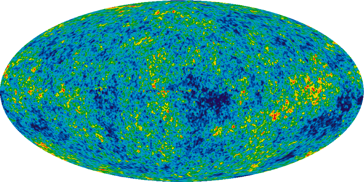
Figure 1.1: Detailed, all-sky picture of the infant Universe created from WMAP. The color scale illustrates initial temperature fluctuations of the CMB ($\sim 13.77\times 10^{9}$ yr old) that correspond to seeds which grew to become galaxies.This image shows a temperature range of $±200$ microKelvin. Credit: NASA/WMAP Science Team

The Matter dominated era began around 500 thousand years after the Big Bang ($z\sim 1000$), when the temperature dropped to $\sim 3000$ K. The temperature was low enough to allow the binding of free electrons with hydrogen and helium nuclei (recombination) – the baryonic gas became neutral. Matter and radiation decoupled and the Universe “brightened” becoming transparent to light. The photons at this recombination stage were free to propagate through the Universe. This process continues until nowadays – as testified by the (ever-fading) cosmic blackbody radiation: cosmic microwave background radiation (CMB). The latter shifted gradually through the infrared to the radio spectral range. Its local fluctuations are measured by Wilkinson Microwave Anisotropy Probe (WMAP) (Fig. 1.1). The Universe entered the so called “Dark ages”, period for which little or nothing is known. The first stars and galaxies lit up the Universe and brought the end of the “Dark ages”. In the period between redshifts 15 (age of $2.7\times 10^{8}$ years) and 7 (age of $7.8\times 10^{8}$ years) the first massive stars produced heavy elements which might have been ejected in the interstellar medium through supernovae explosions. The first stars and quasars probably generated enough ultraviolet radiation to reheat and re-ionize the surrounding Universe (the process known as reionization). The ionized gas containing primordial baryons was enriched by heavy elements, produced in stars. This gas environment is known as all pervading intergalactic medium (IGM). During the non-linear formation of structures, the IGM became clumpy and highly inhomogeneous. It provided material for star formation and, on the other hand, was an environment where heavy elements and energy were ejected.

The baryonic evolution of the Universe. Problems.

According to the current Lambda cold dark matter ($\Lambda$CDM) cosmological model, the Universe consists of baryonic matter ($\approx$ 4 per cent) and “cold” dark matter ($\approx$ 25 per cent) that interacts only gravitationally but does not emit electromagnetic radiation. The remaining $\sim$ 70 per cent of the Universe is the fraction of dark energy conceived as anti-gravity that causes acceleration of the expansion of the Universe. The nature of dark matter and dark energy is still unclear and thus these components are matter of intensive research. It is believed that the distribution of baryonic matter follows the one of the dark matter in form of dark-matter halos.

Although the fraction of baryonic matter is small, it is of key significance to understand the structure and the evolution of the Universe. The standard big-bang nucleosynthesis theory (SBBN) predicts the primordial abundances of helium-3, helium-4, deuterium and lithium-7 (a nucleus of 3 protons and 4 neutrons), depending on a single parameter: the dimensionless baryon density $\Omega_{\rm b}$, i.e. the baryon density normalized to the critical density of the Universe. There are various ways to estimate this parameter which put to test the value predicted by the SBBN and enable the study of the baryon evolution of the Universe. A large literature presenting different results on baryon density has been accumulated within the last decades.

One of the methods to estimate $\Omega_{\rm b}$ is through measurement of the deuterium-to-hydrogen ratio (D/H). In the early 1970s, Reeves et al. (1973) pointed out that deuterium can be produced only during the Big Bang or other pre-galactic event and suggested that the Big bang is the main mechanism for its formation. Those authors concluded that the deuterium abundance sets an upper limit to the baryon density. A few years later Adams (1976) suggested for first time that the amount of deuterium in intergalactic clouds can be measured by use of Lyman absorption spectra (see Sect. 1.3) of distant quasi stellar objects (QSOs; see Sect. 1.2). Afterwards, many efforts have been made to determine the baryon density from deuterium abundance (e.g. Carswell et al., 1994; Songaila et al., 1994; Tytler et al., 1996). About two decades later Burles & Tytler (1998) measured the deuterium-to-hydrogen ratio by analysis of a Lyman limit absorption system (see Sect. 1.3) at $z\sim 3.6$ and asserted that their result is consistent with the primordial value from the SBBN. Using the obtained estimate of D/H in the framework of the SBBN theory, they derived the total baryon density in the Universe: $\Omega_{\rm b}h^{2}=0.0193\pm 0.0014$ (where $h=H_{0}/100$ km s^-1 $\rm Mpc^{-1}$).

In the late 1990s, other attempts to determine the baryon density of the Universe have been made from measuring the Ly-$\alpha$ alpha forest (see Sect. 1.3.1) flux decrement $D\equiv\langle 1-e^{-\tau}\rangle$, i.e. the mean absorbed fraction of the QSO continuum, by use of the relation between $\Omega_{\rm b}$ and the optical depth $\tau$ (see Eq. 8 in Weinberg et al., 1997). A flux decrement distribution was obtained in the work of Rauch et al. (1997), based on observations in the redshift range $2.52\leq z\leq 4.55$ and on simulations. The derived value from the baryon content in the Ly-$\alpha$ forest was $\Omega_{\rm b}h^{2}=0.021\pm 0.017$.

About 10 years ago Netterfield et al. (2002) estimated the baryon density through analysis of the peaks of the CMB angular power spectrum. At $z=0$ the cosmic blackbody radiation has cooled down to temperature of $\approx 3$ K and thus has shifted to the microwave range. The amplitudes and the positions of CMB peaks are sensitive to photon and baryon content – from their measured values one can derive the expected total baryon density and other fundamental cosmological parameters of the early Universe. Netterfield et al. (2002) obtained $\Omega_{b}h^{2}=0.022\pm 0.003$, in a good agreement with the SBBN prediction, and came to conclusion that their results confirm the standard cosmological model of structure formation. A very similar estimate of the total baryon density was done later by Huey et al. (2004): $\Omega_{b}h^{2}=0.025\pm 0.002$. In addition, some very resent studies of the CMB angular power spectrum from WMAP yield values in the range $0.019\leq\Omega_{b}h^{2}\leq 0.024$ ($0.039\leq\Omega_{b}\leq 0.049$, for $h=0.7$), with 95 per cent confidence and in consistency with the SBBN (Lahav & Liddle, 2010). Comparing estimates of the total baryon density in the Universe (Burles & Tytler, 1998; Netterfield et al., 2002; Lahav & Liddle, 2010) and the measured baryon content at high redshifts (Rauch et al., 1997; Weinberg et al., 1997), it seems that the latter, as detected in the Ly-$\alpha$ forest, accounts for nearly all of the total $\Omega_{b}$.

On the other hand, the baryon content at $z=0$ can be measured by summing up the amounts in different observable structures which are baryon tracers: stars, galaxies, galaxy groups and galaxy clusters. The mass of the latter can be directly estimated by use of the mass-to-light ratio. Fukugita (2004) argue that 6 per cent of the baryons at zero redshift are contained in stars and star remnants, 8 per cent are in galaxies and 4 per cent are concentrated in rich clusters of galaxies. Shull et al. (2012) find that 5 per cent of the baryon content is in ionized circumgalactic medium (CGM), surrounding the galaxies, and 1.7 per cent is in cold neutral atomic H i gas, which can be detected through surveys in the 21 cm line.

Obviously, the richest “containers” of baryons in the Universe are to be sought among other objects. Shull et al. (2012) estimate that 28 per cent of the baryons at $z=0$ are comprised in the photoionized Ly-$\alpha$ forest ($T<10^{5}$). Besides that cool, photoionized gas, there exists a hot intergalactic gas with temperatures $T\sim 10^{5}-10^{7}$ K and with low densities $n\sim 10^{-6}-10^{-4}$ cm^-3, called Warm-Hot Intergalactic Medium (WHIM). The WHIM is believed to be a shock-heated and collisionally ionized gas, originating from a collapsing medium driven by the gravity of the large-scale filaments (Cen & Ostriker, 1999; Davé et al., 2001; Valageas et al., 2002). The contribution of WHIM at $z=0$ to the total baryon budget, estimated from O vi absorptions (see Danforth & Shull, 2008; Tilton et al., 2012) and broad Ly-$\alpha$ (BLA) absorption lines (see Richter et al., 2004, 2006), is $\approx$ 30 per cent (Shull et al., 2012). On the other hand, summing up the fractions in the baryon budget at $z=0$ of galaxies, CGM, intracluster medium (ICM), cold neutral gas, photoionized Ly-$\alpha$ IGM gas and the WHIM, Shull et al. (2012) found that $\approx 30$ per cent of the baryons (in comparison to the total expected amount), are not observed. It seems that part of the baryons at low redshift is missing. This “missing baryons problem” was first presented by Fukugita et al. (1998) who derived a value of $\Omega_{b}(z=0)=0.021$, a factor of 2 lower than the total expected baryon content.

Another still unresolved issue with matter content in the Universe is known as the “missing metal problem” at high redshift, formulated originally by Pettini (1999). In astrophysics, all elements heavier than hydrogen and helium are traditionally labeled “metals”. Observations of young stars in distant galaxies at various redshifts provide an opportunity to trace the evolution of star formation rate, i.e. the star formation history (SFH), up to $z\approx 7$. Hence, assuming some initial stellar mass function, one can estimate the expected metal production rate and the density of cosmic metals $\Omega_{Z}^{\rm SFH}$ at given $z$ (Ferrara et al., 2005). On the other hand, an observational estimate of metal content $\Omega_{Z}^{\rm obs}$ at high redshifts can be derived from studies of Ly-$\alpha$ forest, damped Ly-$\alpha$ absorbers (DLAs) (see 1.3.1) and Lyman break galaxies (LBGs) as demonstrated by Pettini (1999). The comparison of $\Omega_{Z}^{\rm SFH}$ with $\Omega_{Z}^{\rm obs}$ shows that 80 per cent of the expected metal content is not detected at $z>2$, i.e. $\Omega_{Z}^{\rm obs}\leq 0.2\leavevmode\nobreak\ \Omega_{Z}^{\rm sfr}$ (Ferrara et al., 2005).

1.2 The importance of studying the IGM

The IGM is built up form filaments of ionized gas outside the galaxies. Recent studies demonstrate that it can be located inside as well outside the hosting dark matter halos (Mo et al., 2010). Properties of intergalactic clouds can be studied best measuring their absorption of light from extragalactic background sources like QSOs. Some QSOs are very distant active galactic nuclei with sizes about the one of the Solar system and bolometric luminosities $\sim$100 times those of normal galaxies (Hoyle et al., 2000). They exhibit a well defined, flat continuum spectrum within a very large spectral range. When an intergalactic gas cloud is located at the sightline toward the QSO, it is detected through absorption lines at certain wavelengths imposed on the QSO continuum. Since some QSOs are located at distances corresponding to redshifts beyond $z=6$, the analysis of their absorption spectra can reveal the properties of the IGM when the Universe was less that 10 per cent of its present age (Mo et al., 2010).

The study of IGM is important for several reasons:

1. It can throw light on the problems of “missing baryons” and “missing metals”. Predictions of some cosmological simulations show that $\approx 30-40$ per cent of the “missing baryons” at $z=0$ are to be comprised in the WHIM (Cen & Ostriker, 1999; Davé et al., 2001). Most of the “missing metals” at $z=2-3$ should be also found there (Cen & Chisari, 2011).

2. The IGM provides the material for galaxy formation through large-scale gas condensations. After the formation of a galaxy, the IGM and the ISM have interacted actively. Gas from the IGM can be accreted into the galaxy and flow into the ISM. And vice versa, gas from the ISM can be ejected and flow back into the IGM. Moreover, the dark-matter halo can cause accretion from the IGM into the large-scale galactic environments (Mo et al., 2010). Thus, the knowledge of the IGM is crucial for understanding galaxy formation and evolution.

3. Basic physical properties of the IGM like temperature, density, chemical composition, ionization state etc. are affected by radiative and gas-dynamical processes. Therefore the study of the IGM can provide information about the cosmological events after the recombination, during the Matter dominated Era.

4. One should take into account the possible interaction of IGM gas particles with CMB photons and, hence, the possible distortion of the CMB spectrum. A good understanding of the IGM is necessary to extract correct information from the CMB.

5. The IGM absorption spectra along the sightline of distant QSOs provide valuable information which can be used to test the evolution of fundamental physical constants like the fine-structure constant $\alpha$, comparing given redshifted atomic or molecular lines with the ones measured in earth bound laboratories (Petitjean et al., 2009; Srianand et al., 2009; Uzan, 2011).

1.3 Quasar absorption line systems as tracers of the IGM

1.3.1 Types of absorption line systems

Various types of absorbing systems are identifiable in QSO spectra that are characterized by a prominent Ly-$\alpha$ emission line and a well-defined continuum from the background source. A typical QSO spectrum at $z=1.34$ is displayed in Fig. 1.2. The QSO’s redshifted emission lines Ly-$\alpha$ and Ly-$\beta$ are clearly visible at $\sim 2400$ Å and $\sim 2850$ Å; various absorption lines are observed blueward of Ly-$\alpha$ emission line.

The traditional classification of absorption systems distinguishes between intrinsic and intervening systems. The intervening systems are located randomly along the QSO sightline and are not related to it. On the other hand, broad and narrow absorption systems in the vicinity of the QSO ($z_{\rm abs}\approx z_{\rm qso}$), are believed to be intrinsic (physically connected) to it. Narrow intrinsic absorbers within separation velocity of $|\Delta v|\equiv(v_{\rm qso}-v_{\rm abs})<5000$ km s^-1 are called in this work associated systems (Weymann et al., 1979; Foltz et al., 1986; Anderson et al., 1987).

Since hydrogen is the most abundant element, the absorber type along the sightline can be characterized through the column density of the neutral hydrogen, $N(\mbox{H\,{\sc i}\leavevmode\nobreak\ }\!\!)$ [cm^-2]:

Ly-$\alpha$ Forest

Clouds of neutral hydrogen which lie along the sightline absorb Ly-$\alpha$ photons of wavelength 1215.67 Å. Due to the various redshifts to these clouds, the corresponding absorption lines are redshifted by factor of $(z+1)$ and detected at various wavelengths blueward of the Ly-$\alpha$ ​​ emission of the QSO. These lines are narrow and appear as a “forest” of lines (Fig. 1.2). The H i column densities of Ly-$\alpha$ forest absorbers span the range $10^{12}-10^{17}$ cm^-2. The lower column density limit reflects the detection limits of the observations, while the upper limit is conditioned by the absorbers’ optical depth – systems with $N(\mbox{H\,{\sc i}\leavevmode\nobreak\ }\!\!)\approx 10^{17}$ are optically thick to Lyman continuum radiation and appear as Lyman limit systems (see below). Mo et al. (2010) point out that, according cosmological simulations, Ly-$\alpha$ forest systems with $N(\mbox{H\,{\sc i}\leavevmode\nobreak\ }\!\!)\geq 10^{14.5}$ cm^-2  are associated with higher density filaments which connect collapsed objects, while Ly-$\alpha$ systems with $N(\mbox{H\,{\sc i}\leavevmode\nobreak\ }\!\!)$ below this value inhabit low density regions. These authors suggest that Ly-$\alpha$ forest absorbers with high column density are possibly enriched with metals from star formation processes in collapsed objects and their low column density peers seem to be more primordial in origin.

The Ly-$\alpha$ forest evolves from high to low redshifts. In the range $2\leq z\leq 5$, the number of Ly-$\alpha$ absorbers per unit redshift is large but rapidly decreasing, mostly due to the expansion of the Universe and partly due to the growth of the large-scale structures (Charlton & Churchill, 2000). At $z<2$, the intensity of extragalactic UV background radiation drops due to the decrease of star-formation rate and of the QSOs space density. (See Sect. 1.3.2 for more details on UV background radiation.). As a result, the fraction of neutral gas contained in Ly-$\alpha$ absorbers increases. The decrease of UV radiation density counteracts the decrease of matter density and thus the absorbers’ number in the Ly-$\alpha$ forest decreases less rapidly than expected from the Universe expansion alone (Mo et al., 2010).

Figure 1.2: A typical QSO spectrum (PKS$0454+039$, at $z=1.34$) with absorption lines produced by galaxies and intergalactic material. The two strongest absorbers (associated with galaxies) are a damped Ly-$\alpha$  absorber at $z=0.86$ and a Lyman limit system at $z=1.15$. The former produces a Lyman limit break at $\sim 1700$ Å and the latter a partial Lyman limit break at $\sim 1950$ Å since the neutral hydrogen column density is not large enough for it to absorb all ionizing photons. Many absorption lines are produced by the DLA at $z=0.86$ (C iv 1548, for example, is redshifted onto the red wing of the quasar’s Ly-$\alpha$  emission line). [Adopted from Charlton & Churchill (2000)]

Lyman Limit Systems

Lyman limit systems (LLS) are rare narrow-line systems which are optically thick at wavelength 912 Å, corresponding to the H i ionization potential of 13.6 eV. They can be detected as saturated Ly-$\alpha$ lines which point to column densities distinctly higher than those of Ly-$\alpha$ forest lines: $1.6\times 10^{17}\leq N(\mbox{H\,{\sc i}\leavevmode\nobreak\ }\!\!)\leq 10^{19}$ cm^-2. LLS cause a break at the rest wavelength of 912 Å, which is well distinguishable (Fig. 1.2). It is difficult, however, to determine accurately the column densities of LLS, since the associated Ly-$\alpha$ lines are very saturated. A way to estimate $N(\mbox{H\,{\sc i}\leavevmode\nobreak\ }\!\!)$ is through the strength of the Lyman limit break, but such LLS are very rare, as pointed out by Mo et al. (2010). LLS are associated with strong metal absorption lines and are believed to arise in the gaseous halos of galaxies, which are respectively embedded in DM halos.

Damped Ly-$\alpha$ Absorbers

Damped Ly-$\alpha$ systems (DLAs) exhibit characteristic damping wings due to natural broadening (see 2.1.2), caused by uncertainty of the energy states involved in the transition (Fig. 1.2). They are rare systems with column densities $N(\mbox{H\,{\sc i}\leavevmode\nobreak\ }\!\!)\geq 2\times 10^{20}$ cm^-2. This lower column density limit is historical in origin – technically speaking, any absorber with $N(\mbox{H\,{\sc i}\leavevmode\nobreak\ })\geq 2\times 10^{19}$ cm^-2  will show damping wings. Systems with $10^{19}\leq N(\mbox{H\,{\sc i}\leavevmode\nobreak\ }\!\!)\leq 10^{20}$ are called sub-DLAs. Hydrogen in DLAs at high redshifts is mostly neutral, while it is significantly ionized in sub-DLAs (Mo et al., 2010). Various heavy elements (metals) are also associated with those systems.

DLAs are referred to as the highest overdensity absorbers – it is believed that they form in DM halos. The total amount of gas in DLAs at $z\approx 3$ is comparable to that of luminous matter in present day galaxies (Mo et al., 2010). Along with the presence of metals, this fact suggests that high-redshift DLAs might have provided the material for galaxy formation. Thus, the detected species in DLAs could throw light on the chemical enrichment in protogalaxies and on the subsequent galaxy formation history. Chemical abundance in DLAs can be measured with a high accuracy, since their H i column densities can be precisely measured from analysis of the damping wings and normally no ionization corrections are necessary.

Metal absorption line systems

The QSO spectra often display absorption lines of metals. The most studied metal systems, which have significance for understanding of the IGM, are Mg ii $\lambda\lambda$ 2796, 2800, C iv $\lambda\lambda$ 1548, 1550 and O vi $\lambda\lambda$ 1031, 1037. As it is seen, the first two types have rest-frame wavelengths which are greater than the one of Ly-$\alpha$ ($\lambda_{\footnotesize\mbox{Ly-{$\alpha$}\leavevmode\nobreak\ }\!\!}=1216$ Å). Thus, their absorption lines lie redward of the QSO emission which enables easy identification of those systems. In contrast, O vi lines lie blueward of the QSO emission and are embedded in the Ly-$\alpha$ forest. This leads to difficulties in identification and analysis, especially at high redshifts, where the Ly-$\alpha$ forest is more densely populated. A typical O vi absorption system is shown in Fig. 1.3.

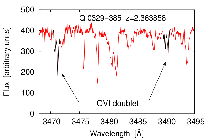
Figure 1.3: A typical O vi system at $z\approx 2.4$: the absorption lines of the doublet $\lambda\lambda\leavevmode\nobreak\ 1031,1037$ along the sightline of a distant QSO.

The ionization potentials of Mg ii ​​ (15 eV), C iv ​​ (65 eV) and O vi ​​ (138 eV) are substantially different. Therefore, the gaseous structures these species are associated with probably inhabit different environments. To produce Mg ii with particle collisions, a temperature of $\sim 10^{4}$ K is necessary, while presence of C iv and O vi in the spectrum requires higher temperatures: $T\sim 10^{5}-10^{6}$ K. Thus lines from different metal ions can reflect the variety of physical conditions in the IGM.

1.3.2 Ionization mechanisms in the IGM

Ionization of the IGM occurs mainly through two mechanisms: ionizing radiation (photoionization) and particle collisions (collisional ionization). We review them briefly below.

Photoionization

Photoionization is a bound-free transition (i.e., a removal of an electron from an atom) due to photon absorption. The rate of this process, $\Gamma_{\rm ph}$, is an integral over all frequencies of the product between the photoionization cross section $\sigma_{\rm ph}(\nu)$ and the number density of ionizing photons at a given frequency. The latter is proportional to the energy flux of the radiation field, i.e., the metagalactic UV background radiation penetrating the IGM. The dominating source is the UV flux from QSOs and young star-forming galaxies, reprocessed and attenuated by the intergalactic gas. According to recent estimates, those objects provide sufficient UV flux to produce the observed ionization level at $z\leq 5$ (Mo et al., 2010; Haardt & Madau, 2012).

The typical lifetime of a hydrogen-like atom is longer than the lifetime of an excited state at low densities. Therefore, the assumption that most photoionizations occur from the ground level is reasonable. The photoionization cross section can be estimated from the formula:

$$\sigma_{\nu,\rm ph}=\frac{C_{0}}{Z^{2}}\Big{(}\frac{\nu_{Z}}{\nu}\Big{)}^{3}g_{1}(\nu)\leavevmode\nobreak\ \leavevmode\nobreak\ \leavevmode\nobreak\ \leavevmode\nobreak\ \leavevmode\nobreak\ \leavevmode\nobreak\ \leavevmode\nobreak\ \leavevmode\nobreak\ \leavevmode\nobreak\ \leavevmode\nobreak\ ({\rm for}\leavevmode\nobreak\ \nu\geq\nu_{Z}),$$ (1.1)

where $Z$ is the atomic number, $\nu_{Z}\equiv\nu_{t}(Z,1)$ is the threshold frequency at the 1^st energy level and $g_{1}$ is the bound-free Gaunt factor for the ground level, which accounts for quantum uncertainties and is close to unity at optical frequencies (Mo et al., 2010). The constant $C_{0}$ does not depend on atomic number and frequency and takes different values on the different sides of the characteristic absorption limits (Kramers, 1923). In the considered case, the constant $C_{0}=7.91\times 10^{-18}$ cm^-2 is determined at the Lyman edge of atomic hydrogen, i.e., it is the Kramers absorption cross section at $\lambda=912$ Å.

Absorption cross sections of multi-electron atoms are described by a more complicated formula. An useful approximation of the contribution of each threshold to the photoionization cross section is:

$$\sigma_{\nu,\rm ph}=a_{t}\Big{[}\beta\Big{(}\frac{\nu_{t}}{\nu}\Big{)}^{s}+(1-\beta)\Big{(}\frac{\nu_{t}}{\nu}\Big{)}^{s+1}\Big{]}\leavevmode\nobreak\ \leavevmode\nobreak\ \leavevmode\nobreak\ \leavevmode\nobreak\ \leavevmode\nobreak\ \leavevmode\nobreak\ \leavevmode\nobreak\ \leavevmode\nobreak\ \leavevmode\nobreak\ \leavevmode\nobreak\ ({\rm for}\leavevmode\nobreak\ \nu\geq\nu_{t}),$$ (1.2)

where a list of numerical values of $\nu_{t}$, $a_{t}$, $s$ and $\beta$ for some atoms and ions can be found in Osterbrock (1989). Then, the total cross section is the sum of individual thresholds. It achieves a maximal value at the threshold and declines with increase of energy.

The photoionization rate of neutral hydrogen is calculated through the formula:

$$\Gamma_{{\scriptsize\mbox{H\,{\sc i}\leavevmode\nobreak\ }\!\!},\rm ph}=4\pi\int\limits_{\nu_{\rm L}}^{\infty}\frac{\sigma_{\nu,\rm ph}J_{\nu}}{\rm h\nu}{\rm d}\nu\approx 2.5\times 10^{-14}J_{-23}\leavevmode\nobreak\ \leavevmode\nobreak\ \leavevmode\nobreak\ \leavevmode\nobreak\ \leavevmode\nobreak\ [\rm s^{-1}],$$ (1.3)

where $J_{\nu}$ is the mean intensity (see Sect. 2.1.1) of the ambient (metagalactic) ionizing radiation field, $\nu_{\rm L}$ is the frequency at the Lyman limit and $\sigma_{\nu,\rm ph}$ is the photoionization cross section of hydrogen. $J_{-23}$ is the dimensionless mean intensity of the UV background intensity at the Lyman limit in units $\rm 10^{-23}\,erg\leavevmode\nobreak\ cm^{-2}\leavevmode\nobreak\ s^{-1}\leavevmode\nobreak\ Hz^{-1}\leavevmode\nobreak\ sr^{-1}$ . $J_{-23}\sim 1-2$ for $z=0$ and much higher ($J_{-23}\sim 80$) for $z=3$.

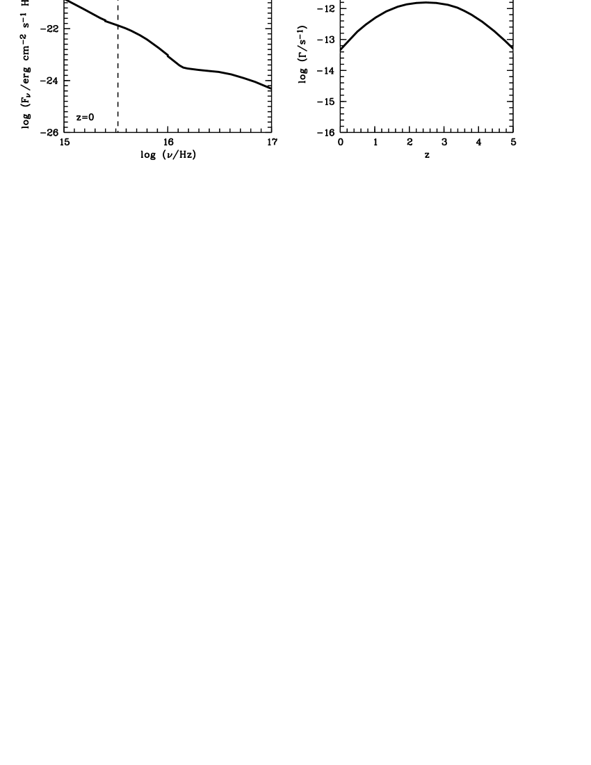
Figure 1.4: Left panel: Spectrum of the metagalactic UV background at $z=0$ (from Haardt & Madau, 1996). The Lyman limit is marked with A dashed line. Right panel: Photoionization rate as a function of redshift. [Adopted from Richter et al. (2008), see the references therein.]

On the left panel of Fig. 1.4 is shown the flux of the metagalactic UV background (see Sect. 2.1.1) at $z=0$ against the frequency $\nu$. The redshift dependence of the hydrogen photoionization rate from the metagalactic UV background is shown on the right panel of the figure.

Collisional ionization

Collisional ionization is another type of bound-free transition, a removal of an electron from an atom due to collision with other particles, predominantly electrons. It is a cooling process since part of the particle kinetic energy is used for ionization. The rate of collisional ionization, $\Gamma_{\rm col}$, is an integral over all velocities $v$ of the colliding electron of the product between the collisional ionization cross section $\sigma_{\rm col}(v)$, the number density of the colliding electrons (which does not depend on $v$) and the velocity distribution. If the velocity distribution is Maxwellian, then the rate and the cross section depend only on the electron energy. The collisional ionization cross section is zero at the threshold energy, $I$, required to unbind the electron and increases with increase of the electron energy. For low energies $I<E\leq 3I$, it can be estimated by use of the approximate formula (Draine, 2011):

$$\sigma_{\rm col}(E)\approx C\pi a^{2}_{0}\Big{(}1-\frac{I}{E}\Big{)},$$ (1.4)

where $C$ is a constant of order unity (for hydrogen, $C=1.07$) and $a_{0}\equiv\hbar^{2}/4\pi^{2}m_{e}q^{2}_{e}$ is the Bohr radius. At higher, but still non-relativistic energies, the collisional ionization cross section decreases as $1/E$.

Recombination and ionization balance

Radiative recombination is a process of free-electron capture by an ion after collision. The collided particles recombine into neutral or weakly-ionized atom, consuming part of their kinetic energy. Therefore radiative recombination is a cooling mechanism. The velocity distribution of electrons in local thermal equilibrium is Maxwellian and the recombination rate depends only on electron temperature and density. The radiative recombination coefficient $\alpha$ at given level is obtained as the average of recombination cross section over the velocity distribution (Boardman, 1964). For hydrogen-like atoms with atomic number $Z>1$, its physical behavior is described by (de Boer, 2007):

$$\alpha_{\rm rad}(Z,T)\approx\frac{T_{e}^{-1/2}}{Z^{2}},$$ (1.5)

In the process of recombination, the excess energy can be absorbed by another bound electron which moves to an excited level and frees its place for the captured one. This phenomenon is called dielectronic recombination. In that case, the recombination coefficient is given by the approximate formula (de Boer, 2007):

$$\alpha_{\rm di}(T)=d_{1}T^{1/2}e^{d_{2}/T},$$ (1.6)

where $d_{1}$ and $d_{2}$ are constants, available in a tabulated form.

The total ionization rate, $\Gamma_{\rm tot}$, is the sum of rates of photoionization, collisional ionization and charge exchange (in case the colliding atoms exchange charge):

$$\Gamma_{\rm tot}=\Gamma_{\rm ph}+\Gamma_{\rm col}+\Gamma_{\rm{charge\leavevmode\nobreak\ exch.}}$$ (1.7)

On the other hand, the total recombination rate, $[\alpha(T)n_{e}]_{\rm tot}$, is the sum of rates of radiative recombination, dielectronic recombination and of charge exchange:

$$[\alpha(T)n_{e}]_{\rm tot}=(\alpha_{\rm rad}+\alpha_{\rm di})n_{e}+\alpha_{\rm charge\leavevmode\nobreak\ exch.}n_{x}\leavevmode\nobreak\ ,$$ (1.8)

where $n_{e}$ is the volume density of electrons and $n_{x}$ – the volume density of charge exchanging particles. The radiative (first) terms dominate in both considered total rates (Eqs. 1.7 and 1.8). Then the ionization balance is governed by the ratio of total ionization and recombination rates (de Boer, 2007):

$$\frac{n_{\rm ion}}{n_{\rm atom}}=\frac{\Gamma_{\rm tot}}{[\alpha(T)n_{e}]_{\rm tot}},$$ (1.9)

The ionization balance is achieved under the state of local thermodynamic equilibrium (LTE). In ionized regions of the ISM and the IGM the electron density depends mainly on the ionization state of hydrogen and $n_{e}\approx n_{p}$. At high electron densities, the ionization balance keeps metals at lower ionization stages.

Collisional ionization equilibrium

Collisional ionization equilibrium (CIE) is the balance between the rates of collisional ionization from the ground level and of recombination from the higher ionization stages at given temperature. In a state of CIE, the fraction of free electrons $X=n_{e}/n$ depends only on the gas temperature. Charge-exchange reactions can be neglected in case of collision between a hydrogen atom and an electron and then the fraction of neutral hydrogen $f_{\scriptsize\mbox{H\,{\sc i}\leavevmode\nobreak\ }}=n_{\scriptsize\mbox{H\,{\sc i}\leavevmode\nobreak\ }}/n_{\scriptsize\rm\mbox{H}}$ is equal to:

$$f_{{\scriptsize\mbox{H\,{\sc i}\leavevmode\nobreak\ }\!\!},\rm col}=\frac{\alpha_{\rm H}(T)}{\beta_{\rm H}(T)},$$ (1.10)

where $\alpha_{\rm H}(T)$ is the recombination coefficient and $\beta_{\rm H}(T)$ is the collisional ionization coefficient, which is the product of electron volume density, the collisional cross section and the velocity distribution of the colliding electrons. The latter in the considered case is Maxwellian and depends only on the electron temperature.

The neutral hydrogen fraction in the WHIM ($T=10^{5}-10^{7}$ K), assuming CIE, can be approximated by (Richter et al., 2008):

$$\log f_{{\scriptsize\mbox{H\,{\sc i}\leavevmode\nobreak\ }\!\!},\rm col}\approx 13.9-5.4\log T+0.33(\log T)^{2}.$$ (1.11)

That gives a vanishing neutral hydrogen fraction of $\sim 2.4\times 10^{-7}$ in CIE at $T=10^{6}$ K.

The ionization states in CIE of typical tracers of WHIM like oxygen, neon, etc., depend only on the gas temperature. Then the fraction of given ion of such element (e.g., five-times ionized oxygen) is determined by the ionization potential of the corresponding ionization level. The temperature dependence of fractions of high ions of oxygen and neon in CIE (based on calculations by Sutherland & Dopita, 1993) is illustrated in Fig. 1.5.

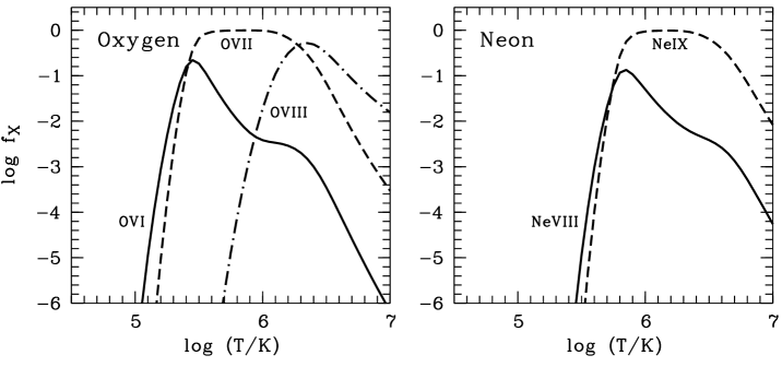
Figure 1.5: CIE ion fractions of selected high ions of oxygen (O vi , O vii , O viii ; left panel) and neon (Ne viii , Ne ix ; right panel) in the WHIM temperature range log ($T/\rm K=4.5-7.0$). Adopted from Richter et al. (2008, see the references therein).

1.4 The case of O vi absorbers

1.4.1 Why it is particularly interesting to study intervening O vi ​​ absorbers?

There are at least several reasons that make the study of five-times ionized oxygen (O vi ​​) interesting and worth of effort:

1. It is believed that the “missing baryons” at low redshifts are hidden in the WHIM (cf. Sect. 1.2), a diffuse medium with temperatures $10^{5}<T<10^{7}$ K. Such warm-hot gas can be traced by highly ionized heavy elements – the latter are usually not fully ionized under such conditions and still undergo electron transitions. In particular, O vi absorption is very important for studying the WHIM. The O vi ion fraction peaks at $T\approx 3\times 10^{5}$ K in CIE and thus this species can probably trace the low temperature regions of the WHIM.

2. The “missing metals” at high redshifts (cf. Sect. 1.2) are probably hidden in hot gaseous highly ionized halos around star-forming galaxies (Ferrara et al., 2005; Richter et al., 2008). The extragalactic UV background is intensive at high redshifts and most of the O vi systems are likely photoionized. However, collisional ionization due to galactic winds could also take place in them (Fangano et al., 2007). This makes O vi systems good candidates for tracing the highly ionized metal enriched halos.

3. Since O vi can be good tracers of metal-enriched ionized gas in the filamentary IGM and in the circumgalactic environment, the analysis of intervening O vi ​​ absorbers towards low- and high-redshift QSOs can be crucial for a better understanding of the physical nature, distribution and evolution of the IGM and its relation to galaxy evolution.

   Let us mention as well two methodological benefits of study of O vi systems:

4. O vi is relatively abundant, while other highly ionized species which can be used as tracers of hot environments, like Ne viii ​​ or N v ​​, have lower cosmic abundance and their detection is more difficult.

5. The doublet O vi $\lambda\lambda 1031,\,1037$ is strong and can be identified relatively easily at low redshifts. Its identification is possible with a high accuracy even at high redshifts, although it is hampered by denser Ly-$\alpha$ forest.

1.4.2 Previous studies of O vi absorbers: advance in our knowledge and unresolved problems

In general, the detected absorbers, including O vi ​​, are classified either as galactic, i.e. associated with a galaxy, or as intergalactic, i.e. located in the IGM. It is commonly accepted that the H i absorbers with $N(\mbox{H\,{\sc i}\leavevmode\nobreak\ }\!\!)\leq 10^{16}$ cm^-2  are associated with intergalactic O vi absorbers, while the galactic O vi absorption is mainly seen in LLSs and DLSs. Although it should be noted that the discrimination galactic/intergalactic is not strict. For instance, some of the Galactic O vi high-velocity clouds (clouds moving with velocities $|v_{\rm LSR}|>100$ km s^-1 through the extended gaseous halo of the Milky Way) are probably intergalactic clouds in the Local Group rather than objects being associated with the Milky Way (Richter et al., 2008). According to a review presented by Fox (2011), at least 775 galactic and intergalactic O vi absorbers can be found in the literature, out of which 328 are low ($z<0.5$) and high ($z\geq 2.0$) redshift intergalactic, both intervening and associated, absorbers (see Sect. 1.3.1).

The O vi doublet $\lambda\lambda 1031,\,1037$ can be detected at low redshift with high-resolution UV spectrographs, such as Goddard High Resolution Spectrograph (GHRS), Space Telescope Imaging Spectrograph (STIS), Cosmic Origins Spectrograph (COS), installed on the Hubble Space Telescope (HST) or Far Ultraviolet Spectroscopic Explorer (FUSE). The review of Fox (2011, see the references therein) lists 25 studies on low-redshift intergalactic intervening O vi absorbers, based on individual sightline detections through UV spectrographs, and a few more survey works by use of all available data. As already mentioned, such systems are often related to the WHIM and their analysis is used extensively to constrain the baryon content of the low-redshift WHIM, mostly under the assumption that they are collisionally ionized (e.g. Tripp et al., 2000; Savage et al., 2002; Richter et al., 2004; Sembach et al., 2004, see Richter et al. 2008 for a review). However, the origin of the O vi absorbing gas phase is still not well known. An important clue to our understanding is the relation between intergalactic intervening O vi ​​ absorbers and the large-scale distribution of galaxies. Wakker & Savage (2009) pointed out that intergalactic O vi absorbers at low redshift preferably arise within 550 kpc of an $L>0.25L_{\star}$ galaxy, with expected metallicities higher than those far away from the galactic structure. Stocke et al. (2006) found no evidence for O vi in intergalactic voids, i.e., at distances $>1.4$ Mpc from the nearest $L>L_{\star}$ galaxy. In view of the last result, Richter et al. (2008) suggest that a local analogue of intergalactic intervening O vi ​​ might be the galactic O vi high-velocity clouds in the Local Group. Sembach et al. (2003) estimated that 60 per cent of the sightlines contain high-velocity O vi clouds with $N(\mbox{O\,{\sc vi}\leavevmode\nobreak\ }\!\!)\geq 2.5\times 10^{13}$, and 36 per cent have $N(\mbox{O\,{\sc vi}\leavevmode\nobreak\ }\!\!)\geq 10^{14}$ cm^-2 (see Fig. 1.6) which corresponds to hydrogen ion densities $N(\mbox{H\,{\sc ii}\leavevmode\nobreak\ }\!\!)\geq 1.2\times 10^{18}$ cm^-2 and $N(\mbox{H\,{\sc ii}\leavevmode\nobreak\ }\!\!)\geq 4.6\times 10^{18}$ cm^-2 respectively, assuming a gas metallicity of $0.2\leavevmode\nobreak\ Z_{\odot}$. Their results indicate that high-velocity O vi ​​ absorbers contain a significant fraction of baryons in the form of warm-hot circumgalactic gas, which might be the local counterparts of intergalactic intervening O vi absorbers at low redshift. Sembach et al. (2003) suggest that collisions in hot gas are the dominating ionization mechanism being responsible for production of the high-velocity O vi ​​.

However, despite the apparent relation between O vi absorbers and the WHIM under the assumption of collisional ionization and the possible local analogue of O vi high-velocity collisionally ionized clouds, recent observational and theoretical studies indicate that part of the low-redshift intervening O vi ​​ absorbers in the IGM may trace low-density, photoionized gas rather than a shock-heated WHIM (Tripp et al., 2008). Also, a simple estimate of the ionization state of the gas from the observed O vi ​​/H i ratios in absorbers can lead to incorrect results because of the complex multi-phase character of the gas (Tepper-García et al., 2011).

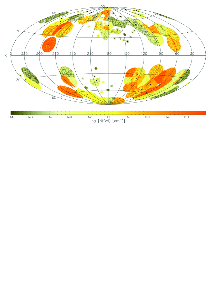
Figure 1.6: All-sky Hammer-Aitoff projections of the high velocity O vi column densities at $z=0$ (the Galactic anticenter is at the center of the plot, and Galactic longitude increases from right to left). Detections are plotted as colored circles with a radius of $12^{\circ}$; in cases of overlapping (either along the same sightline or along adjoining sightlines), the shaded area size is adjusted accordingly. [Adopted from Sembach et al. (2003)]

At redshift $z\approx 2$, the detection of O vi absorbers is possible in the optical regime and can be measured using high-resolution spectrographs installed on ground-based telescopes like Keck and the Very Large Telescope (VLT). There are three main surveys of high redshift ($z\geq 2$) intergalactic O vi absorbers (Simcoe et al., 2002; Bergeron & Herbert-Fort, 2005; Fox et al., 2008). At least 14 systems have been studied by analysis of individual sightlines; several other works make use of the pixel optical depth method for search of O vi absorbers (see the references in Fox, 2011). Yet, the physics of O vi absorbers at high redshifts remains unclear until today. Photoionization seems to be a suitable ionization mechanism for most of them (Carswell et al., 2002; Bergeron et al., 2002; Bergeron & Herbert-Fort, 2005). On the other hand, some studies suggest that a significant fraction of the intergalactic O vi absorbers may be collisionally ionized (Simcoe et al., 2002, 2006). Numerical simulations indicate that shock-heating by collapsing large-scale structures is not efficient at high redshifts to provide a widespread warm-hot intergalactic phase in the early Universe (e.g., Theuns et al., 2002; Oppenheimer & Davé, 2008). Instead, galactic winds probably represent the major source of collisionally ionized O vi absorbers at higher redshift, enriching the IGM with heavy elements at high gas temperatures (Fangano et al., 2007; Kawata & Rauch, 2007). Bergeron & Herbert-Fort (2005) found evidence of two distinct populations of intergalactic O vi absorbers: metal-poor systems that trace the large-scale IGM, and metal-rich, associated with star-forming and wind-blowing galaxies. However, these results need to be confirmed by use of a larger O vi sample and through cosmological simulations. We investigate this problem using both observational data and simulations in Sect. 3.3, Sect. 4.2.1 and Sect. 5.2.4.

Recent studies on the evolution of intergalactic O vi absorbers from low to high redshifts indicate that the mean column density of these systems evolves only weakly over cosmic times, while the line widths are systematically broader at low $z$ compared to high redshift (Fox, 2011; Muzahid et al., 2012). The latter issue is addressed in Sect. 5.1.3, making use of observational and simulated data. The insensitivity of the mean $N(\mbox{O\,{\sc vi}\leavevmode\nobreak\ }\!\!)$ to the redshift can be explained by the dominance of photoionization as ionization mechanism only, if the average density of the O vi gas is approximately 20 times higher at $z=2.3$ than at $z=0.2$ and the high-redshift absorbers have smaller sizes, lower metallicities, or lower ionization fractions (Fox, 2011). Another possible scenario that might explain this phenomenon is radiative cooling of initially hot shock-heated diffuse gas passing through the so-called ”coronal regime“ ($T\sim 10^{5}-10^{6}$ K) and producing O vi ​​. Heckman et al. (2002) demonstrate that the column density of collisionally ionized and radiatively cooling coronal gas is independent of the total volume density. To explain the characteristic mean $N(\mbox{O\,{\sc vi}\leavevmode\nobreak\ }\!\!)$, the radiative cooling scenario requires a cooling flow speed of 20 km s^-1 for single-phase gas, or multiphase gas with approximately 5 interfaces (between cooler and hotter gas) of $N\sim 10^{13}$ cm^-2  each (Fox, 2011). A better understanding of the ionization mechanism of high-redshift O vi absorbers clearly is desirable. We investigate this issue in Sect. 3.2, 4.3 and 5.3.

1.5 Scientific objectives of the thesis

A) A case study of two intervening O vi ​​ absorbers from high-resolution observations.

As mentioned in the previous section, the mechanisms of ionization for producing high-redshift O vi absorbers may be manifold. A plausible physical picture suggests that low density absorbers are photoionized by the UV background, while collisional ionization dominates in denser regions. The temperature of the O vi gas is the most important parameter related to the relevant ionization mechanism. In view of thermal line broadening, the upper limit $T_{\rm max}$ can be directly estimated from the line width as measured through the Doppler parameter $b$ (see Eq. 2.23). A comparison between $T_{\rm max}$ and the estimate $T_{\rm col}$ from collisional ionization models allows us to distinguish between photoionization and collisional ionization as dominant mechanisms. However, an accurate measurement of the Doppler parameter is necessary. Previous surveys of high-redshift O vi absorbers (Bergeron et al., 2002; Simcoe et al., 2002; Carswell et al., 2002; Bergeron & Herbert-Fort, 2005) have shown that many narrow absorbers with Doppler-parameters $b\leq 10$ km s^-1 do exist. They are to be associated with photoionized gas with $T<10^{5}$ K. However, many high-ion absorbers have a complex nature and are often composed of several velocity subcomponents. Therefore spectral resolutions higher than $R\gtrsim 45,000$ are required to detect narrow components. Hence, our first goal is to analyze data form Ultraviolet and Visual Echelle Spectrograph (UVES) with $R\approx 75,000$ (Sect. 2.3.1) of a single QSO sightline to test whether high spectral resolution is crucial for full component decomposition of the overall structure of particularly complex O vi absorption systems and to obtain reliable results on their ionization conditions. Moreover, high-resolution data are important to achieve completeness of their Doppler-parameter distribution towards the lower end ($b<6$ km s^-1).

B) Detailed analysis of intergalactic O vi samples from UVES observations and OWLS simulations.

The second main goal of this thesis is to perform a detailed analysis of a large O vi sample along 15 high-redshift QSO sightlines using UVES spectra, and comparing it with a sample of O vi absorbers from high- and low-redshift cosmological OverWhelmingly Large Simulations (OWLS; Sect. 2.3.2). The objectives are to address the following issues:

• Origin and nature of high-redshift O vi absorbers

  The problem of the ionization mechanism of O vi absorbers still remains unsolved. Combining observables like column density and Doppler parameter from the large UVES sample with photoionization modeling with Cloudy (see Sects. 2.2.3, 4.3 and 5.3.2) we aim to shed light on whether photoionization is the dominant ionizaion mechanism or not. Further, in Sects. 4.2.1, 4.2.2 and 5.2.4, we want to investigate the possible existence of two O vi ​​ populations as proposed by Bergeron & Herbert-Fort (2005). Also, the OWLS synthetic spectra provide valuable information about physical parameters of the O vi absorbers like temperature, space density and metallicity. Therefore, a comparison between observational and simulated spectra is a powerful method to understand the nature and the origin of high-redshift O vi absorbers (see Sect. 5).

• Metal and baryon fractions at high redshifts traced by intergalactic intervening O vi absorbers

  It is believed that the study of high-redshift O vi absorbers can lead to a solution of the “missing metals problem” (Richter et al., 2008). A contribution of this work is to collect more information about O vi as tracers of matter (Sect. 1.1). We aim to estimate the fractions of baryons and metals at high redshift that are traced by intergalactic O vi systems (Sect. 4.2.3 and 5.4).

• Possible differences in origin and nature between low- and high-redshift O vi ​​ absorbers

  Cosmological evolution of O vi absorbers is a further issue that needs a better understanding. We address this issue by comparing observables (column density and Doppler parameter) and physical parameters like temperature, volume density and metallicity at $z=0$ and $z>2$ (Sect. 5).

Chapter 2 Analysis techniques and spectral data

2.1 Basics of absorption lines spectroscopy

We review briefly here some basic physical quantities and processes that are used in the analysis of absorbing systems. All information about the processes in the IGM is based on the detected radiation; in particular, on the absorption line spectra. In this chapter we present some elements of the theory of radiation, the important line broadening mechanisms and some methods and tools of absorption spectroscopy.

2.1.1 Elements of the theory of radiation

Below we review some photometric quantities, the interaction between radiation and matter and the equation of radiative transfer.

Basic notions

• Specific intensity $I_{\nu}$ is defined as the rate of radiation energy flow $dE_{\nu}/dt$ per unit frequency interval $d\nu$, per unit area $dS$ and per unit solid angle $d\Omega(\theta,\phi)$:

  $$I_{\nu}(\theta,\phi)=\frac{dE_{\nu}}{dS\leavevmode\nobreak\ dt\leavevmode\nobreak\ d\nu\leavevmode\nobreak\ d\Omega}=\frac{dE_{\nu}}{dA\leavevmode\nobreak\ cos\theta\leavevmode\nobreak\ dt\leavevmode\nobreak\ d\nu\leavevmode\nobreak\ d\Omega}\leavevmode\nobreak\ \leavevmode\nobreak\ \leavevmode\nobreak\ \leavevmode\nobreak\ \leavevmode\nobreak\ [\rm J\leavevmode\nobreak\ m^{-2}\leavevmode\nobreak\ s^{-1}\leavevmode\nobreak\ Hz^{-1}\leavevmode\nobreak\ sr^{-1}],$$ (2.1)

  where $\theta$ is the (polar) angle between the sightline and the normal vector to $dS$, $\phi$ is the azimuthal angle and $dA$ is the unit area. Equation 2.1 defines the monochromatic specific intensity as a pencil of radiation. The total specific intensity is the integral over all frequencies:

  $$I=\int\limits_{0}^{\infty}I_{\nu}\leavevmode\nobreak\ d\nu\leavevmode\nobreak\ \leavevmode\nobreak\ \leavevmode\nobreak\ \leavevmode\nobreak\ \leavevmode\nobreak\ [\rm J\leavevmode\nobreak\ m^{-2}\leavevmode\nobreak\ s^{-1}\leavevmode\nobreak\ sr^{-1}].$$ (2.2)

• Mean intensity $J_{\nu}$ is the average of specific intensity over all solid angles:

  $$J_{\nu}=\frac{1}{4\pi}\oint I_{\nu}\leavevmode\nobreak\ d\Omega=\frac{1}{4\pi}\int\limits_{0}^{2\pi}\leavevmode\nobreak\ d\phi\leavevmode\nobreak\ \int\limits_{0}^{\pi}\leavevmode\nobreak\ {I_{\nu}\leavevmode\nobreak\ \rm sin}\theta\leavevmode\nobreak\ d\theta\leavevmode\nobreak\ \leavevmode\nobreak\ \leavevmode\nobreak\ \leavevmode\nobreak\ \leavevmode\nobreak\ [\rm J\leavevmode\nobreak\ m^{-2}\leavevmode\nobreak\ s^{-1}\leavevmode\nobreak\ Hz^{-1}\leavevmode\nobreak\ sr^{-1}].$$ (2.3)

  Using the designation $\mu={\rm cos}\theta$, one obtains $\oint d\Omega=-\int\limits_{0}^{2\pi}\leavevmode\nobreak\ d\phi\int\limits_{+1}^{-1}d\mu=\int\limits_{0}^{2\pi}\leavevmode\nobreak\ d\phi\int\limits_{-1}^{+1}d\mu$ and hence:

  $$J_{\nu}=\frac{1}{4\pi}\int\limits_{0}^{2\pi}\leavevmode\nobreak\ d\phi\int\limits_{-1}^{+1}I_{\nu}(\mu,\phi)\leavevmode\nobreak\ d\mu.$$ (2.4)

  In plane-parallel media the radiation field is independent on $\phi$ (symmetry in regard to the $Z$-axis) and then the mean intensity can be written in the form:

  $$J_{\nu}=\frac{1}{2}\int\limits_{-1}^{+1}I_{\nu}(\mu)\leavevmode\nobreak\ d\mu.$$ (2.5)

  It follows from equation 2.5 that if the specific intensity is isotropic, i.e. independent of $\theta$, then $J_{\nu}=I_{\nu}$.

• Physical flux $F_{\nu}$ is the net rate of radiation energy flow from all directions per unit area, per unit time and per unit frequency interval:

  $$F_{\nu} = \oint I_{\nu}\leavevmode\nobreak\ {\rm cos}\theta\leavevmode\nobreak\ d\Omega=\int\limits_{0}^{\pi}d\theta\leavevmode\nobreak\ \int\limits_{0}^{2\pi}\leavevmode\nobreak\ d\phi\leavevmode\nobreak\ I_{\nu}\leavevmode\nobreak\ {\rm cos}\theta\leavevmode\nobreak\ {\rm sin}\phi$$

  $$= \int_{0}^{2\pi}d\phi\int_{-1}^{+1}\leavevmode\nobreak\ I_{\nu}(\mu,\phi)\leavevmode\nobreak\ \mu\leavevmode\nobreak\ d\mu\leavevmode\nobreak\ \leavevmode\nobreak\ \leavevmode\nobreak\ \leavevmode\nobreak\ \leavevmode\nobreak\ [\rm J\leavevmode\nobreak\ m^{-2}\leavevmode\nobreak\ Hz^{-1}].$$ (2.6)

  In plane-parallel media, this formula is simplified:

  $$F_{\nu}=2\pi\int_{-1}^{+1}\leavevmode\nobreak\ I_{\nu}(\mu)\leavevmode\nobreak\ \mu\leavevmode\nobreak\ d\mu.$$ (2.7)

  Specific intensity $I_{\nu}$ does not depend on the distance to the source $r$ while $F_{\nu}$ decreases as $r^{-2}$. The specific intensity can be measured only if the source is resolved; otherwise, only the physical flux can be measured.

• Mean radiation energy density $U_{\nu}$ is the energy density per unit frequency interval in a given volume $V$:

  $$U_{\nu}\leavevmode\nobreak\ d\nu=\frac{1}{V}\oint_{V}\oint_{\Omega}dE_{\nu}=\frac{1}{c}\oint_{\Omega}I_{\nu\leavevmode\nobreak\ }d\nu\leavevmode\nobreak\ d\Omega,$$ (2.8)

  or:

  $$U_{\nu}=\frac{1}{c}\oint_{\Omega}I_{\nu}\leavevmode\nobreak\ d\Omega=\frac{4\pi}{c}\leavevmode\nobreak\ J_{\nu}\leavevmode\nobreak\ \leavevmode\nobreak\ \leavevmode\nobreak\ \leavevmode\nobreak\ \leavevmode\nobreak\ \leavevmode\nobreak\ \leavevmode\nobreak\ \leavevmode\nobreak\ [\rm J\leavevmode\nobreak\ m^{-3}\leavevmode\nobreak\ Hz^{-1}]\leavevmode\nobreak\ \leavevmode\nobreak\ \leavevmode\nobreak\ \leavevmode\nobreak\ \leavevmode\nobreak\ \leavevmode\nobreak\ (\rm see\leavevmode\nobreak\ Equation\leavevmode\nobreak\ \ref{eq_mean_intensity}).$$ (2.9)

  The total radiation energy density is the integrated $U_{\nu}$ over all frequencies:
  $U=\int\limits_{0}^{\infty}\leavevmode\nobreak\ U_{\nu}\leavevmode\nobreak\ d\nu$.

• Absorption

  When a radiation ray passes through gas clouds it loses part of its energy through scattering. Photons can be absorbed and re-emitted at different frequency – this process of transformation of radiative energy into other forms is called ”true“ absorption. In another physical case, light intensity decreases due to scattering whereas photons are just redirected without destruction. The absorption coefficient gives the fraction of the total loss of energy in the pencil of radiation due to "true" absorption. It is related to the microphysics of particles – how likely they absorb an incident photon. The change in intensity $dI_{\nu}$ due to true absorption along length unit $ds$ is given in a form:

  $$dI_{\nu}=-\sigma_{\nu}\leavevmode\nobreak\ n\leavevmode\nobreak\ I_{\nu}\leavevmode\nobreak\ ds,$$ (2.10)

  where $n$ is the volume density of absorbing particles and $\sigma_{\nu}$ is the absorption cross-section per particle, which is equivalent to the absorption coefficient in units of area.

  In a homogeneous medium at rest, the absorption coefficient is isotropic. However, if the medium is moving with respect to the observer, $\sigma_{\nu}$ depends on the angle between the photon direction and the radius vector at the point of observation, and on the frequency, due to the Doppler effect.

• Emission

  An increase in the pencil of radiation energy, due to de-excitation of atoms, is called "true" emission. The emission coefficient (or, monochromatic emissivity) $j_{\nu}$ is defined as the energy $dE_{\nu}$ generated per unit volume, per unit time, per unit frequency interval and per unit solid angle:

  $$j_{\nu}=\frac{dE_{\nu}}{dV\leavevmode\nobreak\ dt\leavevmode\nobreak\ d\nu\leavevmode\nobreak\ d\Omega}\leavevmode\nobreak\ \leavevmode\nobreak\ \leavevmode\nobreak\ \leavevmode\nobreak\ \leavevmode\nobreak\ \leavevmode\nobreak\ \leavevmode\nobreak\ \leavevmode\nobreak\ \leavevmode\nobreak\ \leavevmode\nobreak\ [\rm J\leavevmode\nobreak\ m^{-3}\leavevmode\nobreak\ s^{-1}\leavevmode\nobreak\ Hz^{-1}\leavevmode\nobreak\ sr^{-1}].$$ (2.11)

  Hence the increase of the intensity along an elementary length $ds$ is:

  $$dI_{\nu}=j_{\nu}(s)ds.$$ (2.12)

  Like in the case with absorption coefficient, emissivity is isotropic in a homogeneous medium at rest, but is angle dependent and anisotropic in moving medium, due to Doppler shift, aberration and advection.

Equation of Radiative Transfer

The change of specific intensity of radiation energy from point to point is expressed by the equation of radiative transfer. If a beam of radiation passes through intervening material along a path-length $ds$, its change between the points $s$ and $s+ds$ is caused by emission and absorption effects in the medium:

$$dI_{\nu}=(j_{\nu}-k_{\nu}I_{\nu})ds$$ (2.13)

or:

$$\frac{dI_{\nu}}{ds}=j_{\nu}-k_{\nu}I_{\nu}=-k_{\nu}(I_{\nu}-S_{\nu}),$$ (2.14)

where $k_{\nu}\equiv\sigma_{\nu}n/\rho$ is the mass absorption coefficient (or, the opacity per unit mass), $\rho$ is the mass density and $S_{\nu}=j_{\nu}/k_{\nu}$ is the so called source function. In the case of LTE, the source function of the intervening material is equal to the intensity of radiation energy: $S_{\nu}=B_{\nu}(T)$. The latter is called Planck function and depends only on temperature. Hence, in LTE, Kirchhoff’s law holds: $j_{\nu}=k_{\nu}B_{\nu}(T)$.

The product of mass absorption coefficient $k_{\nu}(s)$ and length $ds$ is a measure of the optical thickness of the material, called optical depth: $d\tau_{\nu}=k_{\nu}(s)ds$. The cumulative effect is expressed through the integral along the line of sight: $\tau_{\nu}=\int\limits_{0}^{D}k_{\nu}(s)ds$, where $D$ is the distance of path length. Using this definition, the equation of radiative transfer can be re-written in the form:

$$\frac{dI_{\nu}}{d\tau_{\nu}}=S_{\nu}-I_{\nu}.$$ (2.15)

The formal solution of the radiative transfer equation is:

$$I_{\nu}(s)=I(0)e^{-\tau(s,0)}+\int\limits_{0}^{s}S_{\nu}(s^{\prime})e^{-\tau(s,s^{\prime})}k_{\nu}ds^{\prime},$$ (2.16)

where $\tau_{\nu}(s,s^{\prime})$ is the optical thickness (or depth) of absorbing material between points $s$ and $s^{\prime}$. The equation shows that the radiation intensity at any point and in a given direction is sum of the emissions at all points $0\leq s^{\prime}\leq s$, reduced by the factor $e^{-\tau(s,s^{\prime})}$ which reflects the absorption by the intervening material (Chandrasekhar, 1960).

2.1.2 Line shape and broadening

Let us consider a population of particles of a given element $X$ in an energy state $X_{l}$ and of volume density $n_{l}$ which interacts with a population of photons with intensity $I_{\nu}$. If $E_{l}$ and $E_{u}$ are the energies of the lower and upper energy states of the element, respectively, photons with frequencies $h\nu=E_{u}-E_{l}$ can be absorbed. The relative probability that a photon with frequency $\nu$ will be absorbed can be expressed by definition with the line profile function, $\phi_{\nu}$, normalized so that:

$$\int\phi_{\nu}d\nu=1.$$ (2.17)

From the other hand, the cross section, $\sigma_{\nu}$, is given by:

$$\int\sigma_{\nu}(lu)d\nu=\frac{g_{u}}{g_{l}}\frac{c^{2}}{8\pi\nu^{2}_{ul}}A_{ul}.$$ (2.18)

where $\nu_{ul}=(E_{u}-E_{l})/h$ is the frequency corresponding to the exact energy difference between the levels $u$ and $l$ and $g_{u}$ and $g_{l}$ are their statistical weights. The constant $A_{ul}$ is called Einstein coefficient and it is a measure of probability for spontaneous transition from upper to lower energy state. It is related to the intrinsic properties of the element energy levels. In astrophysics, the absorption-oscillator strength, $f_{lu}$, is often used instead of the Einstein coefficients. The relation between them is:

$$A_{ul}=\frac{8\pi^{2}e^{2}\nu^{2}}{m_{e}c^{3}}\frac{g_{l}}{g_{u}}f_{lu}\leavevmode\nobreak\ \leavevmode\nobreak\ \leavevmode\nobreak\ \leavevmode\nobreak\ \leavevmode\nobreak\ \leavevmode\nobreak\ [s^{-1}].$$ (2.19)

Combining equations 2.17, 2.18 and 2.19, one obtains:

$$\sigma_{\nu}(lu)=\frac{g_{u}}{g_{l}}\frac{c^{2}}{8\pi\nu^{2}_{ul}}A_{ul}\phi_{\nu}=\frac{\pi e^{2}}{m_{e}c}f_{lu}\phi_{\nu}.$$ (2.20)

Clearly, the function $\phi_{\nu}$ contains all the information of how the absorption cross section depends on frequency. In other words, the line profile is simply a representation of this dependency.

Natural broadening

The uncertainty principle says that the momentum (energy, velocity) and the position of a particle can not be precisely determined at the same time. Therefore an intrinsic quantum effect of line broadening takes place: the so called natural broadening. A good approximation of the line profile due to natural broadening is given through the Lorentz profile:

$$\phi_{\nu}\approx\frac{4\gamma_{ul}}{16\pi^{2}(\nu-\nu_{ul})^{2}+\gamma_{ul}^{2}},$$ (2.21)

where $\gamma_{ul}=1/\tau_{u}+1/\tau_{l}=\sum\limits_{j<u}A_{uj}+\sum\limits_{j<l}A_{lj}$ has a dimensionality of frequency and $\tau_{u}$ and $\tau_{l}$ are the lifetimes of the upper and lower energy states, respectively. Thus the profiles of naturally broadened lines can be computed from the Einstein coefficients; their full width at half maxima are $\Delta\nu_{\rm FWHM}=\gamma_{ul}/2\pi$. Typical line widths for allowed optical and UV absorptions, produced by natural broadening, are $\sim 0.01$ km s^-1 ​​.

Doppler broadening

At finite temperature, the vast majority of a particle population has velocities (velocity dispersion) in some limited range. The Doppler effect allows absorption and emission processes in a range of frequencies around the frequency of given line. Therefore a second source of line broadening is the Doppler broadening. For a gas with Maxwellian velocity distribution, the fraction of particles $f_{v}$ in velocity interval $[v,\,v+dv]$ is:

$$f_{v}dv=\frac{1}{\sqrt{2\pi\sigma^{2}_{v}}}e^{-v^{2}/2\sigma^{2}_{v}}dv,$$ (2.22)

where $\sigma_{v}$ is (thermal) velocity dispersion, $\sigma_{v}=\sqrt{kT/m}$. In spectroscopy, the broadening (Doppler) parameter $b=\sqrt{2}\sigma_{v}=\sqrt{2kT/m}$ is widely used instead of the velocity dispersion. Obviously, if the line width is dominated by thermal motions, the gas temperature is directly derived from the Doppler parameter (in km $\rm s^{-1}$) and the atomic mass number $A$ of the element:

$$T(K)=\frac{mb^{2}}{2k}=A\Big{(}\frac{b}{0.129}\Big{)}^{2}\leavevmode\nobreak\ \leavevmode\nobreak\ \leavevmode\nobreak\ \leavevmode\nobreak\ [\leavevmode\nobreak\ {\rm K}\leavevmode\nobreak\ ].$$ (2.23)

The Maxwellian velocity distribution can be transformed in terms of frequency instead of velocity, using the Doppler width $\Delta\nu_{D}=(v/c)\nu_{ul}=(\sqrt{2}\sigma_{v}/c)\nu_{ul}=(\sqrt{2kT/m}/c)\nu_{ul}$ and thus a Gaussian line profile function with dispersion $\sigma_{\nu}=(\sigma_{v}/c)\nu_{ul}$ is obtained:

$$\phi_{\nu}=\frac{1}{\sqrt{2\pi\sigma^{2}_{\nu}}}e^{-\nu^{2}/2\sigma^{2}_{\nu}}=\frac{1}{\sqrt{\pi}\Delta\nu_{D}}e^{-\nu^{2}/\Delta\nu_{D}^{2}}.$$ (2.24)

Some physical conditions require to take into account, besides the thermal motion, the bulk motions in the gas, e.g. turbulent flows. Then the effective Doppler width of a line is a sum of a thermal and a turbulent components:

$$\Delta\nu_{D}^{\rm eff}=\frac{\nu_{0}}{c}\sqrt{\frac{2kT}{m}+v^{2}_{\rm turb}},$$ (2.25)

where $\nu_{0}$ is the centroid frequency of the absorption line.

Under interstellar and intergalactic conditions the effect of Doppler broadening is much greater than that of natural broadening, because the gas speed is typically much higher than $\sim 0.01$ km s^-1 ​​.

Voigt profile

Both natural and Doppler broadening influence the profile of absorption or emission lines. Therefore the true line profile is a convolution of the Gaussian (Eq. 2.24) and Lorentz (Eq. 2.21) profiles. This convolution is the well-known Voigt profile:

$$\phi_{\nu}=\frac{1}{\sqrt{2\pi\sigma^{2}_{v}}}\int\limits_{-\infty}^{\infty}e^{-v^{2}/2\sigma^{2}_{v}}\frac{4\gamma_{ul}}{16\pi^{2}(\nu-(1-v/c)\nu_{ul})^{2}+\gamma_{ul}^{2}}dv.$$ (2.26)

The shape of the Voigt profile consists of a ‘core’, dominated by a Doppler (Gaussian) profile ($\propto e^{-\nu^{2}/2\sigma^{2}_{\nu}}$) and broad ‘wings’, described by a Lorentz profile ($\propto(\nu-\nu_{ul})^{-2}$). This behavior is illustrated in Fig. 2.1.

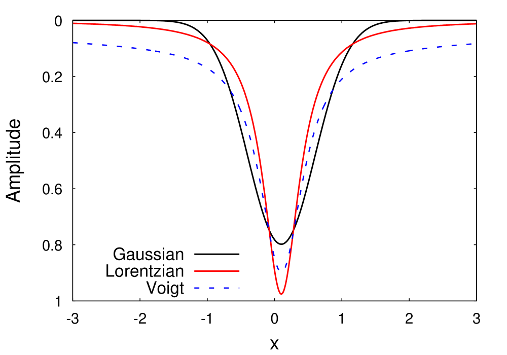
Figure 2.1: Doppler (Gaussian), Lorentz and Voigt line profiles.

Other broadening mechanisms

• Collisional (pressure) broadening

  If the absorbing (or emitting) gas atoms or ions frequently collide with each other, their electron energy levels will be distorted. Subsequently, absorption or emission lines will undergo additional broadening, called collisional or pressure broadening. This effect depends on the frequency of collisions $\nu_{\rm col}=v_{\rm th}n\sigma_{\rm col}\leavevmode\nobreak\ \leavevmode\nobreak\ ,$ where $v_{\rm th}=\sqrt{2kT/m}$ is the thermal velocity of the particles, $n$ is their volume density and $\sigma_{\rm col}$ is their cross section of collisions. The resulting line profile is a Lorentz one, like in the case of natural broadening. Thus both collisional and natural effects can be combined: $\Gamma=\gamma+2\nu_{\rm col}$. The effect of collisional broadening is even smaller than that of natural broadening and does not play a role in the low-density IGM.

• Stark and Zeeman effects

  The Stark and Zeeman effects cause also distortion of the energy levels of gas atoms or ions, due to presence of an external static electric or magnetic fields, respectively. Those effects are not important in the IGM.

2.1.3 Equivalent width and curve of growth

Below we describe briefly some applications of the radiative transfer theory in absorption spectroscopy.

Equivalent width

If a bright continuum point source with intensity $I_{\nu}(0)$ is observed (e.g., star or quasar) within a small solid angle $\Delta\Omega$, then the registered continuum flux $F_{\nu,\rm cont}$, free of any emission and absorption, is: $F_{\nu,\rm cont}=\int I_{\nu}(0)d\Omega=I_{\nu}(0)\Delta\Omega\equiv F_{\nu}(0).$ If the light from the point source passes through a gas cloud, uniform over $\Delta\Omega$, the radiative transfer equation of this system is: $I_{\nu}=I_{\nu}(0)e^{-\tau_{\nu}}+B_{\nu}(T_{\rm ext})(1-e^{-\tau_{\nu}})$, where $T_{\rm ext}$ is the excitation temperature of the intervening material. Hence the actual registered flux is: $F_{\nu}=\int I_{\nu}d\Omega=F_{\nu}(0)e^{-\tau_{\nu}}+B_{\nu}(T_{\rm exc})\Delta\Omega(1-e^{-\tau_{\nu}})$, assuming that the optical depth $\tau_{\nu}$ is constant. The ISM or IGM gas is usually cold, the rate of ionization is much lower than the rate of recombination ($n_{u}/n_{l}\ll 1$) and thus $B(T_{\rm exc})\Delta\Omega\ll F_{\nu}(0)$. Therefore a good approximation of the actual flux is:

$$F_{\nu}=F_{\nu}(0)e^{-\tau_{\nu}}.$$ (2.27)

The optical depth $\tau_{\nu}$ is negligible except in a narrow frequency range and therefore $F_{\nu}(0)$ can be directly measured (outside this range). Knowing $F_{\nu}(0)$ on the two sides of an absorption line, one can estimate $F_{\nu}(0)$ through interpolation even in the range of strong absorption. Therefore, the equivalent width of a line can be defined as:

$$W\equiv\int\limits_{0}^{\infty}\left(\frac{F_{\nu}(0)-F_{\nu}}{F_{\nu}(0)}\right)\frac{d\nu}{\nu_{0}}=\int\limits_{0}^{\infty}\left(1-\frac{F_{\nu}}{F_{\nu}(0)}\right)\frac{d\nu}{\nu_{0}}=\int\limits_{0}^{\infty}(1-e^{-\tau_{\nu}})\frac{d\nu}{\nu_{0}},$$ (2.28)

where $\nu_{0}$ is the line center frequency. The equivalent width can be measured even if the absorption line is not resolved in frequency, since it is a measure of the integrated area of the absorption profile in respect to the unabsorbed local continuum, i.e., $F_{\nu}(0)$. The equivalent widths of two absorption lines of different optical depth is shown in Fig 2.2.

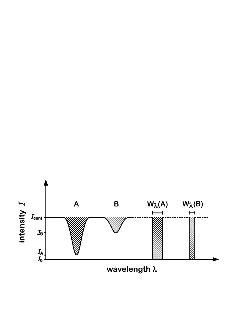
Figure 2.2: Equivalent widths of two absorption lines. [The figure has been kindly provided by Philipp Richter.]

There is a relation between $W$ and column density of absorbers through the optical depth, $\tau_{\nu}$. Using the definition of $\tau_{\nu}$ and 2.20, one obtains:

$$\tau_{\nu}=\int\limits_{0}^{d}k_{\nu}ds=\int\limits_{0}^{d}\sigma_{\nu}n_{l}(s)ds=\frac{\pi e^{2}}{m_{e}c}f_{lu}\int\limits_{0}^{d}\phi_{\nu}(s)n_{l}(s)ds.$$ (2.29)

If the profile function $\phi_{\nu}$ is independent of $s$, the equation above is modified:

$$\tau_{\nu}=\frac{\pi e^{2}}{m_{e}c}\phi_{\nu}f_{lu}\int\limits_{0}^{d}n_{l}(s)ds=\frac{\pi e^{2}}{m_{e}c}\phi_{\nu}N_{l}f_{lu},$$ (2.30)

where $d$ is the length over which the absorption is present (i.e. the absorber size) and $N_{l}$ is the column density of the absorbing gas between the observer and the background source. As it is seen from the Eq. 2.29, $N_{l}=\int\limits_{0}^{d}n_{l}ds$. Typically, the Ly-$\alpha$ forest absorption lines have small column densities ($N_{\footnotesize\mbox{H\,{\sc i}\leavevmode\nobreak\ }\!\!}<10^{15}$cm^-2) and undergo Doppler broadening, thus the Voigt profile can be approximated by a pure Gaussian (Eq. 2.24). The line profile $\phi_{\nu}$ in that case reaches a peak value of $1/\sqrt{2\pi\sigma_{v}^{2}}=1/\sqrt{\pi}b$ at $\nu_{0}=\nu_{ul}$, where $b=\sqrt{2}\sigma_{v}$ is the Doppler broadening parameter. Then the (maximal) optical depth $\tau_{0}$ at the line center $\lambda_{ul}=c/\nu_{0}$ is

$$\tau_{0}=\sqrt{\pi}\frac{e^{2}}{m_{e}c}\frac{f_{lu}\lambda_{ul}N_{l}}{b},$$ (2.31)

while the optical depth in the Doppler part (‘core’) of the line profile is described by

$$\tau_{\nu}=\tau_{0}e^{-u^{2}/b^{2}},$$ (2.32)

where $u=c(\nu-\nu_{0})/\nu_{0}$ is the required velocity shift for producing a frequency shift $\nu$.

Curve of growth

The equivalent width of a line is an increasing function of $\tau_{0}$, depending on the Doppler parameter, the oscillator strength, the wavelength and the column density. The function $W(\tau_{0})$, or $W(N)$ is labeled curve of growth. Three limiting cases of the line profile lead to different behavior of the $W$:

• Optically thin lines ($\tau_{0}\ll 1$)

  In that case the factor $(1-e^{\tau_{\nu}})$ in Eq. 2.28 can be approximated by use of Maclaurin series $e^{x}=\sum\limits_{0}^{\infty}x^{n}/n!$. Hence one obtains for the equivalent width to second order:

  $$W=\int\limits_{0}^{\infty}(1-e^{-\tau_{\nu}})\frac{d\nu}{\nu_{0}}\approx\int\limits_{0}^{\infty}\left(\tau_{\nu}-\frac{\tau_{\nu}^{2}}{2}\right)\frac{d\nu}{\nu_{0}},$$ (2.33)

  The absorption in optically thin lines can described almost always through a Doppler core and therefore $\tau_{\nu}$ can be approximated through a Doppler form (Eq. 2.32). Then the integral 2.33 is obtained straightforwardly:

  $$W=\sqrt{\pi}\frac{b}{c}\tau_{0}\left(1-\frac{\tau_{0}}{2\sqrt{2}}\right).$$ (2.34)

  For small $\tau_{0}$ the second term in the brackets can be neglected and applying Eq. 2.31 the equivalent width in the limit of optically thin lines becomes:

  $$W=\sqrt{\pi}\frac{b}{c}\tau_{0}=\pi\frac{e^{2}}{m_{e}c^{2}}f_{lu}\lambda_{ul}N_{l}.$$ (2.35)

  The constant of proportionality depends only on atomic constants for the considered line. Thus, for a given equivalent width $W$, the corresponding column density $N_{l}$ is directly known. This behavior is illustrated in Fig. 2.3. The linear part of the curve of growth represents the case of optically thin absorption lines. Obviously, the equivalent width in this regime does not depend on the Doppler parameter.

  

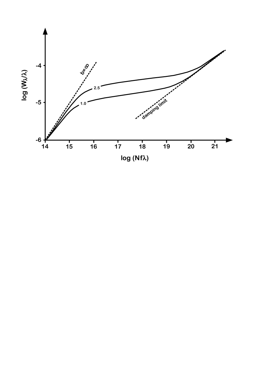
  Figure 2.3: Curve of growth composed from 3 limiting cases of line profile. The solid curves are derived for $b=$ 1.0 and 2.5 km s^-1 ​​. The flat part of the curve corresponds to saturated profiles. For $N(\mbox{H\,{\sc i}\leavevmode\nobreak\ }\!\!)>10^{20}$ cm^-2​​, the profile develops damping wings, which dominate the equivalent width. [The figure has been kindly provided by Philipp Richter.]

• Saturated lines ($\tau_{0}>1$)

  In that case there are no photons with frequencies around the line center available to be absorbed. Therefore only a small fraction of gas particles with velocities essentially different than the most probable speed (away form the line center) contribute to the increase of the equivalent width – adding more absorbers on the sightline would lead to a sub-linear increase of this quantity. The line-profile approximation through the Gaussian ‘core’ (Eq. 2.32) is still possible, but the factor $(1-e^{\tau_{\nu}})$ in Eq. 2.28 is replaced by an inverted ‘top-hat function’: equal to 0 near $\nu_{0}$ and equal to 1, otherwise. Then the full width at half maximum (FWHM) is taken to be the hat width:

  $$\frac{1}{2}=\exp(-\tau_{\rm FWHM})=\exp\big{(}-\tau_{0}e^{-[\Delta u_{\rm FWHM}/2]^{2}/b^{2}}\big{)}.$$ (2.36)

  Solving this equation, one obtains for the equivalent width:

  $$W=\frac{(\Delta u)_{\rm FWHM}}{c}=\frac{(\Delta\nu)_{\rm FWHM}}{\nu_{0}}=\frac{2b}{c}\sqrt{\rm ln(\tau_{0}/\rm ln2)}.$$ (2.37)

  As expected, this formula shows that $W$ increases as the square root of the log $N_{l}$ (see Fig. 2.3).

• Optically thick (damped) lines ($\tau_{0}\gg 1$)

  In this case, the saturation around the line center extends beyond the Doppler ‘core’. Therefore, a good approximation of the line profile is to consider only its Lorentzian part:

  $$\tau_{\nu}=\frac{\pi e^{2}}{m_{e}c}N_{l}f_{lu}\frac{4\gamma_{lu}}{16\pi^{2}(\nu-\nu_{0})^{2}+\gamma_{lu}^{2}}.$$ (2.38)

  Inserting this relation into Eq. 2.28 is obtained:

  $$W=\int\limits_{0}^{\infty}\left(1-{\rm exp}\left[-\frac{\pi e^{2}}{m_{e}c}N_{l}f_{lu}\frac{4\gamma_{lu}}{16\pi^{2}(\nu-\nu_{0})^{2}+\gamma_{lu}^{2}}\right]\right)\frac{d\nu}{\nu_{0}},$$ (2.39)

  which solution is:

  $$W=\sqrt{\frac{e^{2}}{m_{e}c^{2}}N_{l}f_{lu}\lambda_{lu}\left(\frac{\gamma_{lu}\lambda_{lu}}{c}\right)}=\sqrt{\frac{b}{c}\frac{\tau_{0}}{\sqrt{\pi}}\frac{\gamma_{lu}\lambda_{lu}}{c}},$$ (2.40)

  Thus, in the limiting case of damped lines the equivalent width is proportional to the square root of column density: $W\propto\sqrt{N_{l}}$ (see Fig. 2.3).

2.2 Methods and tools of analysis

2.2.1 Absorption line measurement techniques

There are different ways to estimate the column density of absorbing gas, depending on the considered line characteristic: analyzing the optical depth, fitting Voigt profiles to absorption lines, or examine equivalent widths and constructing curve of growths. Below we present some of the most common techniques:

• The curve-of-growth method

  The curve of growth can be used to measure column densities of different species. This method is efficient for low-resolution data wherein the line profile is not resolved. In principle, the recorded line shape is a convolution between the intrinsic shape and the instrumental broadening function. The instrumental broadening is caused by the imperfection of the optical systems of the telescope and the spectrograph. If it is larger than the intrinsic line width the information about the line width is lost. However, the equivalent width is independent on the instrumental broadening, since the latter effect only redistributes $W$ over frequency, without changing its value. Thus, by measuring $W$, it is possible to recover the column density $N$ of an absorber from the linear part and the square-root part of the curve of growth. The logarithmic part of the curve does not provide a good estimate of $N$. In general, if a line is not resolved and its shape can not be directly reproduced, the optical depth at the line center is unknown. Then it is unknown to which part of the curve of growth the considered species belong: the same value of $W$ can imply smaller or larger $N$, for larger or smaller values of the Doppler parameter, respectively.

  However, the problem with unknown optical depth at the line center can be solved by use of doublet or multiplet transitions. A line doublet is observed when transitions are possible from an absorbing state $l$ to two different exited states $u_{1}$ and $u_{2}$ with a small energy separation due to the atomic fine structure. If the spectral resolution is good enough, both equivalent widths of the doublet lines can be measured. In the considered three limiting cases, their ratio is determined only by the known atomic constants. Thus this ratio provides an information on what part of the curve of growth the doublet is. If several transitions from the same atomic level and with different $f\lambda$ take place, an empirical curve of growth can be constructed and hence estimates of $N$ and $b$ can be obtained as well.

• The Voigt-profile-fitting method

  In case the resolution of given absorption spectral lines is high enough, i.e., the lines are resolved, the Voigt-profile fitting technique can be applied. It provides the best-fit values of column density, Doppler parameter and redshift for each component of the absorption feature. To apply that technique, a polynomial fit of the QSO continuum is required (for the other methods as well), since the absorption lines are measured in relation to the continuum. Usually, a $\chi^{2}$-minimization is used to decompose the spectrum into several independent Voigt-profile components, as many as necessary in order to make the procedure free from effects of random fluctuations, i.e., to obtain the same value of the $\chi^{2}$-minimum many times with the same setup. The fitting procedure is quite general and can be used for any profile.

• The apparent-optical-depth method

  This method was first introduced by Savage & Sembach (1991). It distinguishes between “true” and “apparent” optical depth. The “true” $\tau_{\nu}$ is the natural logarithm of the ratio of the continuum flux $F_{\nu}(0)$ and the actual absorbed flux $F_{\nu}$ (Eq. 2.27). However, the recording instrument has a finite resolution, defined by its spectral spread function, which leads to the already mentioned instrumental broadening. Therefore the actual absorption flux has to be convolved with the spectral spread function, in order to extract information about the observed absorption flux, $F_{\nu,\rm obs}$, which differs from the actual flux $F_{\nu}$. Then the “apparent” optical depth is the natural logarithm of the ratio of the continuum flux $F_{\nu}(0)$ and the absorption flux that includes the instrumental broadening $F_{\nu,\rm obs}$.

  The apparent-optical-depth method is applicable if the absorption lines are weak and not (or, mildly) saturated. It can treat single unsaturated lines, as well doublets and multiplets. The observational data are converted to apparent optical depth and further to apparent column density $N_{a}$ per unit velocity interval. A comparison of different $N_{a}$ for doublets and multiplets enables empirical estimates of the line saturation in the true line profile. The apparent optical depth method provides additional information on the velocity dependence of line saturation.

2.2.2 Absorption line fitting tools

In this section we describe briefly the two fitting tools that we have used for analysis of our observational data (see Sect. 2.3.1). We applied the tool Candalf for handling the high- and intermediate- resolution samples of our case study of two O vi absorbers (see Chapter 3). The other tool, Vpfit, has been applied for fitting the intermediate-resolution observational spectra for our UVES survey (see Chapter 4).

• Candalf

  The Candalf routine is aimed at fitting absorption spectra with a Gaussian profile by use of a standard Levenberg-Marquard minimization algorithm. The program simultaneously fits the continuum and the absorption lines, producing as output ion column densities $N$ and Doppler parameters $b$ for each absorption component. The continuum is modeled as a Legendre polynomials of order up to 4. The one-$\sigma$ fitting uncertainties of the obtained estimates of $N$ and $b$ are calculated using the diagonals of the Hessian matrix.

• Vpfit

  The Vpfit program (Carswell et al., 2003) is created to fit observed normalized absorption spectra with multi-component Voigt profiles. The Voigt profiles are convolved with the instrumental profile and then iteratively fitted to the absorption spectra, until the $\chi^{2}$ value is minimized.

2.2.3 Ionization modeling with Cloudy

The software package Cloudy is a spectral-synthesis code designed for simulation of the physical conditions in astrophysical plasma and of its emission spectra (Ferland et al., 1998), with emphasis on achieving reliable estimates of abundances and luminosities of galactic and extragalactic objects. The emitting gas is not in thermodynamic equilibrium and thus an analytical approach for its physical description cannot be used. Therefore numerical simulations of micro-level processes responsible for the observed spectra are performed. As pointed out by Ferland et al. (1998), the structure and the method of such simulation codes (including Cloudy) are similar: an optically thick slab of gas is divided into zones with approximately constant physical conditions. A given ionization level is maintained by balancing ionization and recombination processes. The former include photoionization, Auger ionization and collisional ionization and the latter are radiative recombination, low- and high-temperature dielectronic recombination, three-body recombination and charge transfer. The important assumptions are that the velocity distribution of the free electrons is Maxwellian and that the kinetic temperature of electrons is determined by balance between heating and cooling processes. The heating sources can be various: mechanical or photoelectric processes, cosmic rays etc. Main cooling mechanism are the inelastic collisions between electrons and other particles.

Cloudy solves simultaneously the radiative transfer equations in the continuum and in the lines. To predict line intensities and column densities, it is required to specify the incident continuum, the gas density and the chemical composition. The code is widely used for analysis of emission and absorption line spectra.

2.3 Spectral data used

2.3.1 Observational data (VLT/UVES)

The observational data set used in this work is composed of intermediate- and high-resolution spectra taken with the UVES spectrograph at the VLT. The VLT, installed at Cerro Paranal (Chile), is designed for visible and infrared observations. It consists of four 8.2-meters Unit Telescopes; when they operate in a combined mode, the VLT provides a light collecting power of 16-meter telescope. The UVES is a high-resolution optical spectrograph, installed on the UT2 of the VLT. The telescope light beam is separated in two arms: UV-to-Blue and Visual-to-Red with maximum resolutions of 80,000 and 110,000, respectively (for more details see Dekker et al., 2000).

The intermediate-resolution data set consists of 15 QSO sightlines of spectra with resolution $R\approx 45000$, corresponding to velocity resolution $\sim 6.6$ km s^-1 FWHM. The data were obtained and reduced as part of the former ESO Large Programme "The Cosmic Evolution of the IGM" which was aimed at study of the IGM at $z=1.5-5$ and along a large number of lines of sight, in order to improve the statistics on intervening absorption line systems (see Sect. 1.3.1) and to derive their physical properties (Bergeron et al., 2002). The wavelength coverage of the intermediate resolution data is $3050-10,400$ Å. The signal-to-noise (S/N) ratio varies between $15$ and $90$ per spectral resolution element.

The high-resolution data set consists of spectra of the quasar PKS 1448$-$232 ($z_{\rm em}=2.208$; $V=16.9$), observed at the VLT with the UVES spectrograph in 2007, in an independent run (program ID 079.A$-$0303(A)). The spectral resolution is $R\approx 75,000$ which corresponds to $\sim 4$ km s^-1 FWHM velocity resolution. The full wavelength coverage is $3000-6687$ Å. The raw data were reduced using the UVES pipeline implemented in the ESO-MIDAS software package. The pipeline reduction includes flat-fielding, bias- and sky-subtraction and a relative wavelength calibration. Then the individual spectra have been corrected to vacuum wavelengths and co-added. The S/N ratio of the high-resolution data is $20-70$ per resolution element.

2.3.2 Numerical simulations (OWLS)

The synthetic spectra, analyzed in this work, are generated from a run of the OWLS. The OWLS are a large set of N-body, Smoothed Particle Hydrodynamical (SPH) simulations of structure formation in the Universe (Schaye et al., 2010). The Gadget III code is used for calculating the gravitational and hydrodynamical forces on the system of particles. The values of cosmological parameters adopted in the runs are typical for a flat $\Lambda$CDM cosmological model and in agreement with the results from 3-year WMAP data: $\Omega_{\rm m}$=0.238, $\Omega_{\rm b}$=0.0418, $\Omega_{\rm\Lambda}$=0.762, $\sigma_{\rm 8}$=0.74, $n{\rm s}$=0.95, $h$=0.73 (Spergel et al., 2007). The OWLS use starformation recipe by Dalla Vecchia & Schaye (2008). Galactic winds from core-collapse SNe are also implemented as described by Dalla Vecchia & Schaye (2008). The descriptions of radiative cooling and heating used in OWLS are described by Wiersma et al. (2009a). Briefly, the cooling rates are computed in the presence of CMB and a Haardt & Madau (2001) model of the UV background radiation. An illustration of the temperature, density and metallicity evolution from $z=3.45$ to $z=0.01$ as predicted by OWLS is shown in Fig. 2.4. More details about OWLS can be found in Schaye et al. (2010) and the references therein.

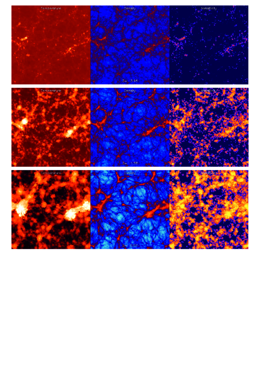
Figure 2.4: The evolution of the ‘cosmic web’ according to the OWLS: in terms of temperature, volume density and metallicity (left to right) and at three different redshifts (top to bottom). Credit: Craig Booth

the OWLS we refer the reader to Schaye et al. (2010).

Detailed information about the computed synthetic spectra can be found in Tepper-García et al. (2011). The spectra were computed by use of the package Specwizard and following the method described by Theuns et al. (1998). Specwizard calculates the optical depths from the velocities along a given sightline and then they are transformed to fluxes at the wavelength of each transition. In that way the observational spectra are modeled and comparable results are achieved. The synthetic spectra, used in this work, are obtained to mimic HST/STIS observations by convolving the spectra with an instrumental Gaussian Line-Spread Function with a FWHM $=7$ km s^-1 and by resampling them onto a 3.5 km s^-1 pixel. Additionally, a Gaussian noise is added by normalizing the flux through different values of the S/N ratio. The reference model in this work (${\rm REF\_L050N512}$) adopts the fiducial value S/N$=50$ per pixel. More details about different reference models are given in Tepper-García et al. (2011); the model, used here, is # 4 in their Table 1 at $z=2.5$, rather that $z=0.25$. In particular, we analyse the physical properties of O vi absorbers found in the synthetic spectra at redshift $z=2.5$.

Chapter 3 A case study of two O vi absorbers
at $z\approx 2$ towards PKS 1448$-$232

In this Chapter, we study in detail two O vi absorption-line systems at $z\approx 2$ in the direction of the quasar PKS 1448$-$232, using two different UVES data sets with different spectral resolutions. Because of its brightness ($V=16.9$), PKS 1448$-$232 ($z_{\rm em}=2.208$) can be observed with UVES at high S/N with relatively moderate observing times. Two prominent O vi systems with redshift $z\approx 2$ have been identified previously (Philipp Richter, priv. comm.), each exhibiting a well-defined velocity-component structure with no major line blending problems. Therefore these two systems are particularly well-suited for a case study of high-redshift O vi absorption.

3.1 Observations and absorption-line analysis

3.1.1 VLT/UVES observations

Our data set for this study consists of intermediate- ($R\approx 45\,000$) and high-resolution ($R\approx 75\,000$) spectra of PKS 1448$-$232 (see Sect. 2.3.1). In Table 3.1 we provide a summary of the observations of PKS 1448$-$232.

Table 3.1: Log of the UVES observations of PKS 1448$-$232: signal-to-noise ratio (S/N), resolution $R$, exposure time, $t_{\rm exp}$, and the wavelength range are listed for both observation runs.

	high res.	intermediate res.
$R$	75,000	42,000
S/N	20$-$70	15$-$90
$t_{\rm exp}$ [min]	780	720
$v_{\rm res}$ [km s-1]	4	7
$\lambda$ range [Å]	3000$-$6687	3050$-$10400

Table 3.2: Fit parameters for the absorbing system at $z=2.1098$

	$z$			O vi		C iv		H i
	O vi	C iv	H i	log[$N$(cm-2)]	$b$ [km s-1]	log[$N$(cm-2)]	$b$ [km s-1]	log[$N$(cm-2)]	$b$ [km s-1]
high resolution data
1	2.10982	2.10982	2.10981	14.27($\pm$0.01)	10.7($\pm$0.2)	13.12($\pm$0.01)	7.5($\pm$0.1)	13.38($\pm$0.04)	19.6($\pm$0.7)
2	2.11011	2.11008	2.11018	13.50($\pm$0.02)	8.4($\pm$0.4)	12.23($\pm$0.03)	6.1($\pm$0.6)	13.37($\pm$0.04)	28.6($\pm$1.7)
intermediate resolution data
1	2.10984	2.10983	2.10981	14.32($\pm$0.02)	10.1($\pm$0.2)	13.12($\pm$0.01)	7.1($\pm$0.1)	13.39($\pm$0.01)	20.6($\pm$0.3)
2	2.11014	2.11008	2.11019	13.49($\pm$0.20)	5.4($\pm$0.5)	12.23($\pm$0.03)	5.3($\pm$0.6)	13.35($\pm$0.01)	26.4($\pm$0.8)

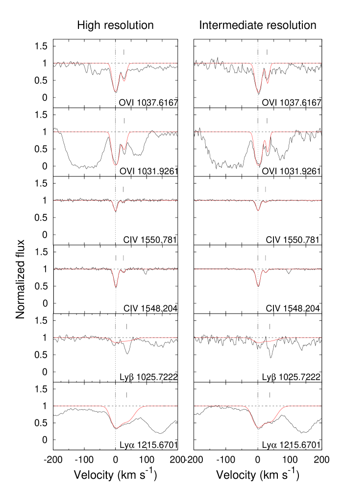
Figure 3.1: Absorption profiles for the O vi absorber at $z=2.1098$ in the high-resolution data (left panel) and the intermediate-resolution data (right panel).

The detected absorption features that are associated with the two absorbers at $z_{\rm abs}=2.1098$ and $z_{\rm abs}=2.1660$ were fitted independently in both spectra (at intermediate and high resolution) with Gaussian profiles using the Candalf fitting routine outlined in Sect. 2.2.2.

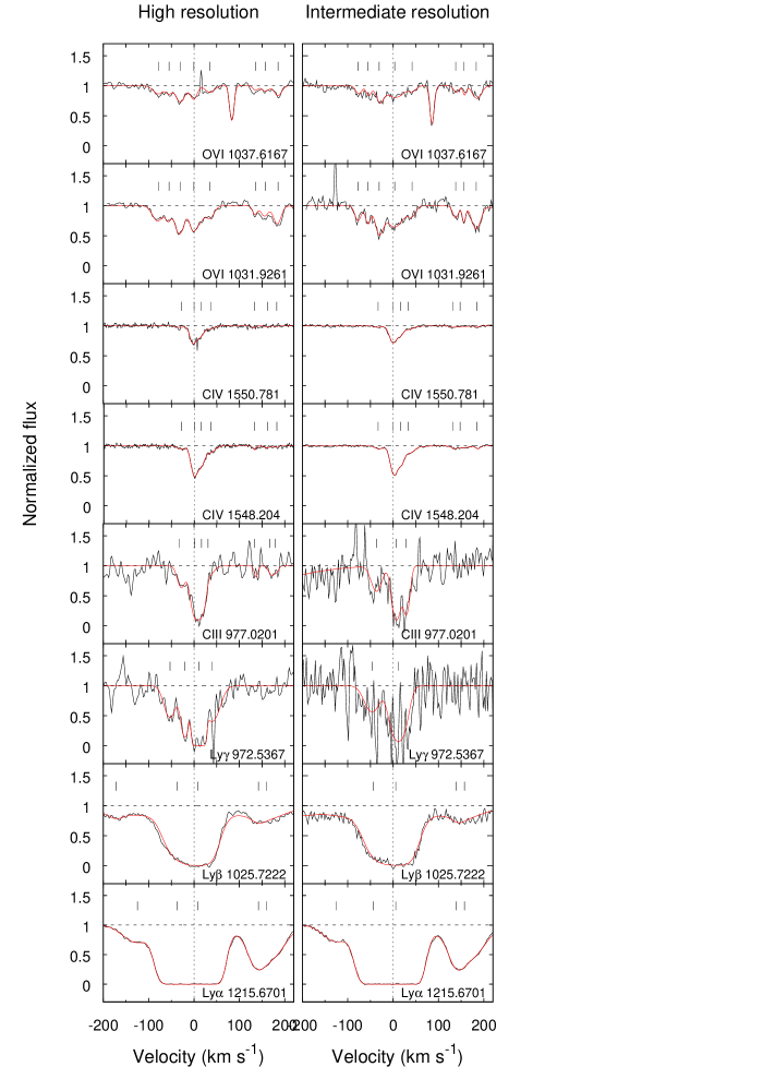
Figure 3.2: Absorption profiles for the O vi absorber at $z=2.1660$ in the high-resolution data (left panel) and the intermediate-resolution data (right panel). The strong absorption observed in O vi $\lambda 1037.62$ plot is a Si iii line at $z=1.7236$.

3.1.2 The O vi system at $z=2.1098$

Fig. 3.1 shows the velocity profiles of O vi ($\lambda\lambda 1031.9,1037.6$), C iv ($\lambda\lambda 1548.2,1550.8$), and H i ​​, Ly-$\alpha$ ​​, and Ly-$\beta$ ($\lambda\lambda 1215.7,1025.7$) for the $z=2.1098$ absorber in the high-resolution data (left panel) and the intermediate-resolution data (right panel). A visual inspection of both panels displays no significant differences between the two data sets. The S/N is on average higher for the high resolution data, except for the O vi region where this ratio is slightly higher at intermediate resolution. Therefore, the differences in the values for $N$, $b$, and $z$ derived for the individual absorption components in the intermediate and high-resolution spectra are a result of the different S/N values for the two data sets.

Two absorption components are detected considering each of these ions. The O vi ​​ absorption is relatively strong compared to C iv ​​. The H i ​​ absorption is weak in comparison with other O vi ​​ absorbers at similar redshift (e.g., Bergeron et al., 2002) with a central absorption depth in the H i line of less than 70 per cent. We note that the second, weaker, component of H i Ly-$\alpha$ and Ly-$\beta$ absorption associated with the high-ion absorption is blended, so that the true component structure of H i as well its relative column density and Doppler parameter values remain somewhat uncertain. The blending aspect is not taken into account in the formal error estimate for $N$ and $b$ given in Table 3.2, which is based on the profile fitting. While the O vi ​​, C iv and H i absorption is well aligned for the stronger component, there appears to be a small ($<10$ km s^-1) velocity shift between H i and the high ions in the weaker one component (see Table 3.2). If real, this shift may indicate that H i and the metal ions may not trace the same gas phase in the weaker absorption component. Owing to the blending of the H i absorption, however, the reality of this shift remains unclear.

For the stronger component, we obtain for column densities log $N$(O vi ​​)$\approx 14.3$, log $N$(C iv ​​)$\approx 13.1$, and log $N$(H i$)\approx 13.4$ as listed in Table 3.2. The resulting ion-to-hydrogen ratios of $N$(O vi ​​)/$N$(H i ​​)$\sim 8$ and $N$(C iv ​​)/$N$(H i ​​)$\sim 0.5$ already indicate that the metallicity of this absorber must be fairly high (Bergeron & Herbert-Fort, 2005). We note that – because of the blending problem in the Ly-$\alpha$ and Ly-$\beta$ lines, – the H i column density may be regarded as an upper limit and thus the ratios given above might be even higher.

Table 3.3: Ly-$\alpha$ fit parameters for the absorbing system at $z=2.1660$

	$z$	log [$N$(H i) (cm-2)]	$b$ [km s-1]
high resolution data
1	2.16466	13.27 ($\pm$0.01)	40.0 ($\pm$1.2)
2	2.16552	14.49 ($\pm$0.07)	29.9 ($\pm$1.2)
3	2.16605	15.18 ($\pm$0.03)	34.9 ($\pm$0.5)
4	2.16746	13.16 ($\pm$0.03)	19.2 ($\pm$0.6)
5	2.16765	13.77 ($\pm$0.01)	45.6 ($\pm$0.3)
intermediate resolution data
1	2.16467	13.21 ($\pm$0.02)	37.4 ($\pm$1.3)
2	2.16559	14.57 ($\pm$0.12)	31.9 ($\pm$1.7)
3	2.16607	15.13 ($\pm$0.05)	35.5 ($\pm$0.8)
4	2.16749	13.19 ($\pm$0.02)	18.8 ($\pm$0.5)
5	2.16768	13.76 ($\pm$0.01)	46.8 ($\pm$0.3)

Table 3.4: Fit parameters for metal lines in the absorber at $z=2.1660$

	$z$			O vi		C iv		C iii
	O vi	C iv	C iii	log[$N$(cm-2)]	$b$ [km s-1]	log[$N$(cm-2)]	$b$ [km s-1]	log[$N$(cm-2)]	$b$ [km s-1]
high resolution data
1	2.16518	—	—	13.35($\pm$0.03)	15.4($\pm$1.3)	—	—	—	—
2	2.16542	—	—	13.02($\pm$0.08)	8.0($\pm$1.2)	—	—	—	—
3	2.16569	2.16569	2.16566	13.63($\pm$0.02)	13.5($\pm$0.7)	12.18($\pm$0.05)	11.1($\pm$1.7)	12.68($\pm$0.07)	11.1a
4	2.16600	2.16600	2.16602	13.41($\pm$0.03)	9.9($\pm$0.6)	13.17($\pm$0.05)	9.3($\pm$0.5)	13.49($\pm$0.05)	15.1($\pm$1.5)
5	—	2.16616	2.16618	—	—	12.96($\pm$0.10)	10.0($\pm$1.6)	12.78($\pm$0.23)	8.0($\pm$3.7)
6	2.16638	2.16638	2.16633	13.21($\pm$0.04)	13.7($\pm$0.8)	12.53($\pm$0.09)	12.6($\pm$2.2)	12.22($\pm$0.47)	12.6a
7	2.16744	2.16741	2.16740	12.75($\pm$0.15)	6.8($\pm$0.8)	11.90($\pm$0.05)	4.8b	12.17($\pm$0.14)	4.8a
8	2.16766	2.16770	2.16780	13.01($\pm$0.16)	10.6($\pm$0.4)	11.84($\pm$0.08)	9.2c	12.32($\pm$0.15)	9.2a
9	2.16796	2.16792	2.16789	13.30($\pm$0.08)	10.9($\pm$1.3)	11.50($\pm$0.12)	4.8b	11.85($\pm$0.36)	4.8a
intermediate resolution data
1	2.16521	—	—	13.12($\pm$0.03)	8.3($\pm$1.0)	—	—	—	—
2	2.16544	—	—	13.13($\pm$0.04)	6.4($\pm$0.9)	—	—	—	—
3	2.16600	2.16567	2.16557	13.53($\pm$0.05)	10.6($\pm$0.9)	12.16($\pm$0.05)	11.1($\pm$1.5)	12.87($\pm$0.11)	14.4($\pm$3.7)
4	2.16606	2.16602	2.16603	13.73($\pm$0.04)	24.8($\pm$3.1)	13.23($\pm$0.02)	10.4($\pm$0.4)	13.39($\pm$0.08)	10.4a
5	—	2.16619	2.16626	—	—	12.73($\pm$0.09)	7.5($\pm$0.9)	13.12($\pm$0.15)	7.5a
6	2.16646	2.16637	2.16635	12.97($\pm$0.11)	10.4($\pm$2.0)	12.67($\pm$0.08)	15.3($\pm$2.6)	—	—
7	2.16748	2.16742	—	12.98($\pm$0.03)	7.3($\pm$0.9)	11.67($\pm$0.17)	4.8($\pm$2.3)	—	—
8	2.16767	2.16758	—	12.93($\pm$0.05)	2.8($\pm$0.9)	12.24($\pm$0.07)	22.2($\pm$3.1)	—	—
9	2.16796	2.16797	—	13.50($\pm$0.01)	12.7($\pm$0.6)	11.85($\pm$0.06)	4.8($\pm$1.2)	—	—

^a Fixed to $b_{\rm C\,{III}}=b_{\rm C\,{IV}}$
^b Fixed to $b$-value derived from the intermediate resolution data
^c Lower limit, fixed to the minimal value

3.1.3 The O vi system at $z=2.1660$

The O vi system at $z=2.1660$ exhibits a significantly more complex absorption pattern than the absorber at $z=2.1098$, as can be seen in the velocity profiles presented in Fig 3.2. We detect O vi absorption in eight individual absorption components, spanning a velocity range as large as $\sim 300$ km s^-1. From our visual inspection, it is evident that the absorption pattern of O vi differs than those of the other detected intermediate and high ions (C iii ​​, C iv ​​) and H i ​​, although some of the components appear to be aligned in velocity space. As for the system at $z=2.1098$, there are no significant differences between the absorption characteristics of the high-resolution data and the intermediate-resolution data. However, the S/N ratio is somewhat lower in the latter for lines that are located in the blue part of the spectrum, hence the resulting fitting values for $N$, $b$, and $z$ for the individual absorption components differ slightly (Tables 3.3 and 3.4).

We modeled the H i absorption by simultaneously fitting Ly-$\alpha$ and Ly-$\beta$ in four absorption components (components $2-5$; see Table 3.3), obtaining column densities in the range $13.2<$  log $N$(H i ​​)$<15.2$. One additional component (component 1) is present in the Ly-$\alpha$ absorption, but is blended in Ly-$\beta$ (see Fig 3.2), so that $N$(H i ​​) was derived solely from Ly-$\alpha$ . We note that for the H i fit we did not attempt to link the H i component structure to the structure seen in the the metal ions, as this requires knowledge about the physical conditions in the absorber. We discuss this aspect in detail in Sect. 3.2.2, where we try to reconstruct the H i absorption pattern based on a photoionization model. We fitted the H i absorption with the minimum number of absorption components required to match the observations (Fig. 3.4, lowest panel) and to obtain an estimate on the total H i column in the absorber.

By summing over the column densities in the individual absorption components, we derive total column densities of log $N$(O vi ​​)$\approx 14.2$, log $N$(C iii ​​)$\approx 13.7$, log $N$(C iv ​​)$\approx 13.5$, and log $N$(H i ​​)$\approx 15.3$. The resulting ion-to-hydrogen ratios of $N$(O vi ​​)$/N$(H i )$\sim 0.1$ and $N$(C iv ​​)$/N$(H i ​​)$\sim 0.02$ (representing the average over all components) are substantially smaller than in the $z=2.1098$ system, which is indicative of a lower (mean) absorber metallicity.

The complexity of the absorption patterns for the various species in this system and the large velocity spread suggests that this absorber arises in an extended multi-phase gas structure.

Table 3.5: Modelled column densities for the absorber at $z=2.1098$

	$v$ [km s-1]	log [$N$ (cm-2)]			log [$n_{\rm H}\,$(cm-3)]	log $Z$	log [$T$(K)]	$L$ [kpc]	$f_{\rm HI}$
		C iv	O vi	H i
1	0	13.12	14.27	13.38	$-$4.20	$-$0.24	4.54	19.9	$-$5.21
2	$+$25	12.23	13.50	13.37	$-$4.25	$-$1.02	4.64	30.5	$-$5.35
2	$+$25	12.23	13.50	12.57a	$-$4.28	$-$0.24	4.57	4.7	$-$5.32

^a Our best H i guess in the model for the second component with fixed metallicity

3.2 Ionization modeling and physical conditions in the gas

To infer information about the physical properties of the two O vi absorbers towards PKS 1448$-$232, we modeled in detail the ionization conditions in these systems. Since the two absorbers at $z=2.1098$ and $z=2.1660$ have redshifts close to the quasar redshift ($z_{\rm QSO}=2.208$), it is necessary to check whether the two systems lie in the proximity of the background quasar and are influenced by its ionizing radiation.

With the above given redshifts, the two absorbers have velocity separations from the QSO of $\delta v_{2.1098}\approx 9000$ km s^-1 and $\delta v_{2.1660}\approx 4000$ km s^-1, thus the absorber at $z=2.1660$ can be regarded (depending on the definition) as an associated system (see Sect. 1.3.1). With a (monochromatic) luminosity at the Lyman limit of $L_{912}=3.39\times 10^{31}$ erg s^-1 Hz^-1, the size of the sphere-of-influence of the ionizing radiation from PKS 1448$-$232 is known to be $6.7$ Mpc, corresponding to a velocity separation of $\sim 1400$ km s^-1 (Fox et al., 2008). Therefore, it is safe to assume that the ionizing radiation coming from PKS 1448$-$232 itself has no measurable influence on the ionization conditions in the two O vi systems.

The small values of the Doppler parameter $b$ measured for O vi ​​, C iv ​​, and H i indicate that collisional ionization is not the source of the O vi existence in the gas. Using Eq. 2.23, we find that the measured Doppler parameters of the O vi components in the two absorbers (all with $b<16$ km s^-1 and many with $b<10$ km s^-1; see Tables 3.2 and 3.4) indicate temperatures $T<10^{5}$ K. This value is below the peak temperature of O vi in CIE ($T\sim 3\times 10^{5}$ K; Sutherland & Dopita, 1993); it is also lower than the temperature range expected for O vi arising in turbulent mixing layers in the interface regions between cold and hot gas ($T=10^{5}-10^{6}$ K; Kwak & Shelton, 2010). Consequently, photoionization by the hard UV background remains as the only plausible origin of O vi in the two high-ion absorbers towards PKS 1448$-$232.

In consideration of this physical picture, we modeled the ion column densities in the two O vi systems using the photoionization code Cloudy (version C08; Ferland et al., 1998) (for details see Sect. 2.2.3). We assumed a solar abundance pattern of O and C and an optically thin plane-parallel geometry in photoionization equilibrium exposed to a Haardt & Madau (2001) UV background spectrum at $z=2.16$, which had been normalized to $\log\leavevmode\nobreak\ J_{912}=-21.15$ (Scott et al., 2000) at the Lyman limit.

We assumed that each of the observed velocity components is produced by a "cloud", which is modeled as an individual entity. As input parameters, we considered the measured column densities of C iii (for only the $z=2.1660$ absorber), C iv ​​, O vi ​​, the metallicity $Z$ (in solar units), and the hydrogen volume density $n_{\rm H}$. The metallicity of each cloud and the hydrogen density were varied across a range appropriate to intergalactic clouds (i.e., $-3\leq\,$log$\leavevmode\nobreak\ Z\,\leq 0$ and $-5\leq\,$log$\leavevmode\nobreak\ n_{\rm H}\leq 0$).

We then applied the following iterative modeling procedure. In a first step, we derived models using Cloudy for a set of values of $Z$, $n_{\rm H}$, and $N$(H i ​​), where $N$(H i ​​) has been constrained by the observations. In a second step, the corresponding values of $N$(C iii ​​), $N$(C iv ​​), and $N$(O vi ​​) were calculated. The output was compared with the observed column densities and, in the case of a mismatch, the input parameters $Z$ and $n_{H}$ were adjusted before the next iteration step. This process was repeated until the differences between the output column densities and the observed values became negligible and we obtained a unique solution. In addition to the ion column densities, our Cloudy model provides information about the neutral hydrogen fraction, $f_{\rm HI}$, the gas temperature, $T$, and the absorption path-length, $L=N$(H i$)/(f_{\rm HI}\,n_{\rm H})$.

3.2.1 The system at $z=2.1098$

As mentioned earlier, absorption by O vi and C iv is well-aligned in both components in this system, while the true component structure of H i is uncertain because of blending effects in the Ly-$\alpha$ and Ly-$\beta$ lines. Owing to the alignment of O vi and C iv ​​, we assumed a single-phase model, in which each of the two components (clouds) at $v=0$ and $+25$ km s^-1 in the $z=2.1098$ rest frame hosts O vi ​​, C iv ​​, and H i of column densities similar to those derived from the profile fitting. Consequently, we assumed log $N$(H i ​​)$=13.37$ and $13.38$ as input for the Cloudy modeling and followed the procedure outlined above. The results of the Cloudy modeling of the $z=2.1098$ absorber are summarized in Table LABEL:tabl_model_2.1098. Our model closely reproduces the observed O vi and C iv column densities in both components, if the clouds have a density of log $n_{\rm H}\approx-4.2$, a temperature of log $T\approx 4.6$, and a neutral hydrogen fraction of log $f_{\rm HI}\approx-5.3$. However, to match the observations, the second component (at $+25$ km s^-1) in our initial model (Table LABEL:tabl_model_2.1098, first two rows) needs to have a metallicity of log $Z=-1.02$, which is $\sim 0.8$ dex lower than that of the other component (log $Z=-0.24$). The absorption path-lengths are $\sim 20$ kpc for the component at $0$ km s^-1 and $\sim 30$ kpc for the component at $+25$ km s^-1.

Taking into account the blending problem for the H i Ly-$\alpha$ and Ly-$\beta$ absorption, which affects in particular the estimate of $N$(H i ​​) in the cloud at $+25$ km s^-1 (Fig. 3.1), we set up a second Cloudy model in which we tied the metallicity of the $+25$ km s^-1 component to the metallicity of the other component (log $Z=-0.24$), but left the $N$(H i ​​) of this component as a free parameter. From this, we derived a value of log $N$(H i ​​)$=12.57$ for the cloud at $+25$ km s^-1 and the absorption path-length decreased to $L=4.7$ kpc. In terms of the blending, we regard this model as more plausible than the model with two different metallicities and to have a larger absorption path-length.

In summary, our Cloudy modeling suggests that the $z=2.1098$ absorber towards PKS 1448$-$232 represents a relatively simple, metal-rich O vi absorber in which the highly ionized O vi and C iv states coexist in a single gas-phase.

Table 3.6: Modelled column densities for the C iii /C iv ​​ absorbing phase in the $z=2.1660$ absorber

	$v$ [km s-1]	log [$N$ (cm-2)]				log [$n_{\rm H}\,$(cm-3)]	log $Z$	log [$T$(K)]	$L$ [kpc]	$f_{\rm H}$
		C iii	C iv	O vi	H ia
3	$-$28	12.68	12.18	10.97	14.51	$-$2.74	$-$1.7	4.42	0.3	$-$3.68
4	$+$0	13.49	13.17	12.25	14.18	$-$2.97	$-$1.7	4.46	4.1	$-$3.95
5	$+$16	12.78	12.96	—	14.51	$-$3.56	$-$1.7	4.58	16.3	$-$4.63
6	$+$37	12.22	12.53	12.86	14.08	$-$3.71	$-$1.7	4.61	12.3	$-$4.79
7	$+$134	12.17	11.90	10.92	13.26	$-$2.93	$-$1.0	4.38	0.04	$-$3.84
8	$+$162	12.32	11.84	10.49	13.57	$-$2.67	$-$1.0	4.34	0.02	$-$3.55
9	$+$182	11.85	11.50	10.38	12.99	$-$2.84	$-$1.0	4.37	0.01	$-$3.73

^a Our best H i guess in the models.

3.2.2 The system at $z=2.1660$

We started to model this system with Cloudy, again under the assumption of a single gas-phase hosting the observed intermediately and highly ionized C iii ​​, C iv ​​, and O vi states in the various subcomponents. However, during the modeling process it quickly turned out that it is impossible to match the observed column densities of C iii and O vi by assuming a single gas-phase in the components, when these two ions are aligned in velocity space. Our modeling indicates that the C iii absorption must instead arise in an environment that has a relatively high gas density and is spatially distinct from the O vi phase. In a second step, we tried to tie the highly ionized C iv and O vi states in a single gas phase (like in the case of $z=2.1098$ system) in the relevant absorption components, ignoring the C iii phase. However, this approach did not deliver satisfying results, as we obtained for some components, for which C iv ​​/O vi was constrained by observations, very low gas densities and very large absorption path-lengths on Mpc scales, which are highly unrealistic. Given that the overall component structures of O vi and C iv differ substantially from each other in this system (Fig. 3.2), this result is not really surprising.

The only modeling approach for which we obtain realistic results for gas densities, temperatures, and absorption path-lengths in this system and its subcomponents is a two-phase model, in which C iii coexists with C iv and part of the H i in one (spatially relatively confined) phase, and O vi and the remainder of the H i in a second (spatially relatively extended) phase. The coexistence of C iii and C iv in one phase is also suggested by the C iii and C iv absorption, which is well- aligned in velocity space (see Fig. 3.2). The results of this two-phase model are presented in Tables LABEL:tabl_model_2.1660 and LABEL:tabl_model_o6_2.1660. A critical issue for the modeling of this complex multi-phase absorber with its many absorption components is the assumption of a neutral gas column density in each subcomponent (and phase). Since in the H i Ly-$\alpha$ and Ly-$\beta$ absorption, most subcomponents are smeared together to one large absorption trough, the observational data provide little information about the distribution of the H i column densities among the individual components. Nevertheless, the data provide a solid estimate of the total H i column density in the absorber (log $N\approx 15.3$; see Sect. 3.1.3), which must match the sum of $N$(H i ​​) over all subcomponents considered in our model. Consequently, we included in our iteration procedure the constraints on $N$(H i )_tot and the shape of the (total) H i absorption profile. The latter aspect also concerns the choice of the gas temperature in the model, as $T$ regulates the thermal Doppler-broadening and thus the width of the modeled H i lines. We modeled the H i width following the approach of Ding et al. (2003).

With these various constraints, we first modeled the C iii ​​/C iv phase in the absorber. However, owing to the extremely complex parameter space, we did not find a unique solution for $(T,n_{\rm H},Z)$ among the individual components, but had to make additional constraints. Since the individual components observed in C iii ​​/C iv are very close together in velocity space, we assumed they all have the same metallicity and, based on the $Z$ range allowed in the model, we set log $Z=-1.5$ for all subcomponents. This model was able to match the observed column densities of these two ions in the individual subcomponents, but did not match closely the overall shape of the overall H i absorption, implying that the metallicity in this absorber is non-uniform among the individual absorption components. Therefore, we refined our model by using two different metallicities, log $Z=-1.7$ for the saturated H i components and log $Z=-1.0$ for the weaker H i components (see Tables LABEL:tabl_model_2.1660 and LABEL:tabl_model_o6_2.1660 for details). Although imperfect, this model delivers a satisfying match between the modeled spectrum and the UVES data.

Adopting this model, we found that the C iii ​​/C iv absorbing components have temperatures between log $T=4.3$ and $4.6$, densities between log $n_{\rm H}=-3.7$ and $-2.7$, and neutral gas fractions between log $f_{\rm HI}=-4.8$ and $-3.6$ (see Table LABEL:tabl_model_2.1660). The absorption path lengths were found to vary between $0.3$ and $16.3$ kpc for the components with log $Z=-1.7$, and between $0.01$ and $0.04$ kpc for the components with log $Z=-1.0$. These numbers suggest that the C iii ​​/C iv absorbing phase resides in relatively small and confined gas clumps. This scenario is consistent with the small turbulent $b$-values of $<6$ km s^-1 for the subcomponents that we derive in our model. We note that in Table LABEL:tabl_model_2.1660, we also list the predicted column densities for O vi ​​, which are typically $1-2$ orders of magnitude below the observed ones in this absorber. This, again, indicates that C iii ​​/C iv and O vi must reside in different gas phases with different physical conditions to explain the observed column densities.

Finally, we modeled the O vi absorbing phase in the $z=2.1660$ absorber, based on the observed O vi column densities. Since we had information for no ions other than H i and O vi that could provide information about the physical conditions in this phase, we fixed the metallicity of the gas to log $Z=-1.7$ and log $Z=-1.0$ (equal to the phase) and constrained the temperature range [$T_{\rm min},T_{\rm max}$] in the Cloudy models based on the observed line widths of O vi (giving $T_{\rm max}$) and the modeling results of the C iii ​​/C iv phase (giving $T_{\rm min}$ for all components except the first two). The results of this model are shown in Table LABEL:tabl_model_o6_2.1660. We derived gas densities in the range log $n_{\rm H}=-4.6$ to $-3.2$ and neutral gas fractions in the range log $f_{\rm HI}=-5.8$ to $-4.6$. The absorption path length was found to vary between $19.8$ and $83.3$ kpc for the components with log $Z=-1.7$, and between $1.3$ and $38.3$ kpc for those with log $Z=-1.0$. The mismatch between $N$(O vi ​​) of the model and the data for components one and nine (see Table LABEL:tabl_model_o6_2.1660) implies that the metallicity distribution among the individual absorption components is even more complex than the one assumed in our model. Despite this (minor) concern, our Cloudy modeling for O vi provides clear evidence that the O vi absorbing phase has substantially lower gas densities than the C iii ​​/C iv absorbing phase and is spatially more extended.

In summary, our Cloudy modeling of the $z=2.1660$ absorber suggests that this system has a complex multi-phase gas structure, in which a number of cooler, C iii ​​/C iv ​​ absorbing cloudlets are embedded in a spatially more extended, O vi absorbing gas phase spanning a total velocity range of $\sim 300$ km s^-1. Although the metallicity is not well-constrained in our model, it appears that log $Z\leq-1$ in the absorber, which is $\sim 0.8$ dex below the value obtained for the system at $z=2.1098$.

Table 3.7: Modelled column densities for the O vi absorbing phase in the $z=2.1660$ absorber

	$v$ [km s-1]	log [$N$ (cm-2)]		log $Z$	log [$T$(K)]	$L$ [kpc]	$f_{\rm H}$
		O vi	H ia	log [$n_{\rm H}\,$(cm${-3}$)]
1	$-$78	12.96b	13.17	$<-$3.76	$-$1.7	$<$5.36	$<$19.8	$>-$5.86
2	$-$55	13.02	14.10	$<-$3.77	$-$1.7	$<$4.79	$<$25.8	$>-$5.03
3	$-$30	13.63	14.51	$-$3.91 … $-$3.31	$-$1.7	4.42 … 5.24	58.4 … 67.7	$-$5.50 … $-4.84$
4	$+$0	13.41	14.18	$-$3.99 … $-$3.88	$-$1.7	4.46 … 4.98	42.6 … 83.3	$-$5.36 … $-$4.95
6	$+$36	13.21	14.08	$-$3.92 … $-$3.23	$-$1.7	4.61 … 5.26	32.1 … 21.5	$-$5.52 … $-$5.00
7	$+$136	12.75	13.26	$-$3.72 … $-$3.72	$-$1.0	4.38 … 4.64	1.3 … 2.0	$-$4.82 … $-$4.61
8	$+$157	13.01	13.57	$-$3.70 … $-$3.52	$-$1.0	4.34 … 5.03	2.2 … 6.1	$-$5.19 … $-$4.56
9	$+$185	13.25c	12.99	$-$4.60 … $-$4.25	$-$1.0	4.37 … 5.06	32.3 … 38.3	$-$5.76 … $-$5.48

^a Our best H i guess in the models
^b Observed log $N$(O vi) $=13.35$
^c Observed log $N$(O vi) $=13.30$

3.3 Discussion

Our detailed analysis of the two O vi absorbers at $z=2.1098$ and $z=2.1660$ towards the quasar PKS 1448$-$232 has clearly illustrated the large diversity and complexity of high-ion absorbers at high redshift.

A number of studies based on both optical observations (e.g., Bergeron et al., 2002; Carswell et al., 2002; Simcoe et al., 2002, 2004, 2006; Bergeron & Herbert-Fort, 2005; Aguirre et al., 2008) and numerical simulations (e.g., Fangano et al., 2007; Kawata & Rauch, 2007) have investigated the properties of high-redshift O vi systems and their relation to galaxies.

As a result of their survey of O vi absorbers at redshifts $z=2.0-2.6$, Bergeron & Herbert-Fort (2005) suggested that O vi systems may be classified into two different types: metal-rich absorbers (“type 1”) that have large $N$(O vi ​​)/$N$(H i ​​) ratios and that appear to be linked to both galaxies and galactic winds, and metal-poor absorbers (“type 0”) with small $N$(O vi ​​)/$N$(H i ​​) ratios, which are embedded in the IGM. The two absorbers observed towards PKS 1448$-$232 that we have discussed in this Chapter do not match the classification scheme of Bergeron & Herbert-Fort (2005). The absorber at $z=2.1098$ has a very large $N$(O vi ​​)/$N$(H i ​​) ratio of $\sim 8$ (i.e., it is of type 1): it is a simple, single-phase, metal-rich system with a metallicity slightly below the solar value. Nevertheless, this system is completely isolated with no strong H i Ly-$\alpha$ absorption within $1000$ km s^-1. In contrast, the absorber at $z=2.1660$ has a $N$(O vi ​​)/$N$(H i ​​) ratio of only $\sim 0.1$ and a metallicity of $0.1$ solar or lower (i.e., it is of type 0 according to Bergeron & Herbert-Fort, 2005). This absorber is a complex multi-phase system with a non-uniform metallicity, suggesting that it originates in a circumgalactic environment. While this mismatch with the Bergeron & Herbert-Fort (2005) classification scheme certainly has no statistical relevance for the general interpretation of O vi absorbers at high redshift, the results suggest that for a thorough understanding of highly-ionized gas at high redshift the absorption characteristics of O vi systems may be too diverse to permit a simple classification scheme based solely on the observed (and partly averaged) column density ratios of O vi ​​, H i ​​, and other ions.

One critical drawback of many previous O vi surveys at high redshift is that they often considered only simplified models for the ionization conditions in their sample of highly ionized absorbers, so that the multi-phase character of the gas and the possible ionization conditions far from a photoionization equilibrium are insufficiently taken into account. As pointed out by Fox (2011), single-phase, single-component ionization models, if applied, will provide physically irrelevant results for most of the O vi systems at high redshift. This implies that previous estimates of the baryon- and metal-content of O vi absorbers at low and high redshift are possibly affected by large systematic uncertainties. We investigate this problem in Sect. 5.3.2

One firm conclusion from many previous observational and theoretical studies of highly ionized absorbers is that a considerable fraction of the O vi systems at low and high $z$ must arise in the metal-enriched circumgalactic environment of (star-forming) galaxies (e.g., Wakker & Savage, 2009; Prochaska et al., 2011; Fox et al., 2011; Tepper-García et al., 2011; Fangano et al., 2007). Thus, the complex absorption pattern observed in the $z=2.1660$ system towards PKS 1448$-$232 and many other O vi absorbers at high $z$ may reflect the complex gas distribution of enriched gaseous material that was ejected from galaxies into the IGM during their wind-blowing phase (e.g., Kawata & Rauch, 2007). In this context, Schaye et al. (2007) suggested that the intergalactic metals were transported from galaxies by means of galactic winds and reside in the form of dense, low- and high-metallicity patches within large hydrogen clouds. These authors point out that much of the scatter in the metallicities derived for high-redshift absorbers could be explained by the spatially varying number of the metal-rich patches and the different absorption path lengths through the surrounding metal-poor intergalactic filament instead of an overall (large-scale) metallicity scatter in the IGM. In this scenario, the substantial differences in the metallicities of the two O vi systems towards PKS 1448$-$232, and even the intrinsic metallicity variations within the $z=2.1660$ system, could be explained by the different geometries of the absorbing structures, suggesting that much of the H i that is associated with the metal absorption in velocity space, arises in a spatially distinct region. In Sect. 5.3.2 we further investigate that problem, using a set of cosmological OWLS. A similar conclusion was drawn by Tepper-García et al. (2011), who studied the nature of O vi absorbers at low redshift using the same set of cosmological simulations. We note that absorbers with larger H i column densities, such as LLS and DLAs, sometimes exhibit abundance variations among the different velocity subcomponents (e.g., Richter et al., 2005; Prochter et al., 2010). This indicates that the metals in the gas surrounding high redshift galaxies have not been well-mixed.

The observed velocity differences between O vi and other ions and the multi-phase nature of the gas provide further evidence of an inhomogeneous metallicity and density distribution in intervening highly ionized absorbers. It is an interesting that the velocity misalignment appears to concern only the O vi absorbing phase in highly ionized absorbers at high redshift, while other highly ionized states such as N v and C iv generally appear to be well-aligned with H i ​​, even in systems that exhibit a complex velocity-component structure (Fechner & Richter, 2009). This puzzling aspect underlines that additional detailed studies of individual O vi absorption systems could be very important to our understanding of intergalactic and circumgalactic gas at high redshift, as this ion traces a metal-enriched gas phase that cannot be observed by other means.

3.4 Conclusions

In this chapter, we investigated two O vi absorbers at $z=2.1098$ and $z=2.1660$ towards the QSO PKS 1448$-$232. For this, we have used high- ($R\approx 75,000$) and intermediate-resolution ($R\approx 45,000$) optical spectra obtained with the VLT/UVES instrument together with Cloudy photoionization models. From our study, we draw the following conclusions:

• The first O vi system at $z=2.1098$ is characterized by strong O vi absorption and weak H i absorption in a relatively simple, two-component absorption pattern. The absorptions by O vi ​​, C iv ​​, and H i are well aligned in the velocity space, indicating that they trace the same gas phase. From a detailed photoionization modeling of this system, we derive a metallicity of $\sim 0.6$ solar, a characteristic density of log $n_{\rm H}\approx-4.2$, a temperature of log $T\approx 4.6$, and a total absorption path length of $\sim 30$ kpc. The absorber is isolated with no strong H i Ly $\alpha$ absorption detected within $1000$ km s^-1.

• The second O vi absorber at $z=2.1660$ represents a complex, multi-component absorption system with eight relatively weak and narrow O vi absorption components spanning almost $300$ km s^-1 in radial velocity. The O vi components are accompanied by a strong H i absorption, and C iii and C iv absorption features. The O vi component structure differs from that of H i and C iv ​​, indicating the absorber contains a multi-phase IGM. Our photoionization modeling with Cloudy suggests that there are (at least) two distinct gas phases in this system. The first consists of C iii ​​, C iv ​​, and most of the H i ​​, which appear to coexist in several relatively compact cloudlets at gas densities from log $n_{\rm H}\approx-3.7$ to $-2.7$, temperatures of log $T\approx 4.3-4.6$, and absorption path-lengths of $<16$ kpc. We have found that O vi appears to reside in a highly ionized, more spatially extended gas phase at densities in the range log $n_{\rm H}\approx-4.6$ to $-3.2$, temperatures between log $T\approx 4.3$ and $5.3$, and absorption path-lengths up to $83$ kpc. While the precise metallicity of the absorber is not well-constrained, our modeling is most consistent with a non-uniform metal abundance in the individual absorption components with (at least) two different metallicities of log $Z=-1.7$ and log $Z=-1.0$.

• Our study illustrates the large diversity and complexity of O vi systems at high redshift. We speculate that some of the observed differences between the studied two highly ionized absorbers towards PKS 1448$-$232 could result from an inhomogeneous metallicity and density distribution in the photoionized IGM. Our study indicates that multi-phase, multi-component highly ionized absorbers similar to the one at $z=2.1660$ can be described by a detailed ionization modeling of the various subcomponents to obtain information about the physical conditions and metal-abundances in the gas.

We conclude that much effort will be required to achieve a more complete view of the nature of O vi absorbers at high redshift. Therefore, the next logical step in this project is to analyze a larger sample of O vi absorbers using high-quality UVES archival data. This analysis will be presented in the following chapter.

Chapter 4 An UVES survey of O vi absorbers at high redshift

The case study of two O vi absorbers towards PKS $1448-232$ presented in the previous chapter indicates the complexity and diversity of highly-ionized intergalactic gas structures at high redshift. However, a much larger sample of O vi absorbers is required to study the nature of these objects on a statistically secure basis and to pinpoint their role in the cosmological gas circulation processes in the early Universe.

In this chapter, we therefore study a larger sample of O vi absorbers from high-quality UVES archival data (see Sect. 2.3.1). These data are publicly available in the UVES data archive and have a spectral resolution of $R\approx 45\,000$ (see Sect. 2.3.1). We further use the O vi absorber list of Dr. Tae-Sun Kim (priv. comm.), who has fitted intervening absorption-lines systems from these data using the Vpfit fitting program (see Sect. 2.2.2).

4.1 Overview of the sample

Following Songaila (2005) and Scannapieco et al. (2006), we define a system as an O vi absorber with at least two components as the separation of each of them from its closest neighbor is $\leq 100$ km s^-1 ​​.

We found 93 candidates for O vi systems in total in 15 inspected sightlines in the composed UVES sample. Fifty three systems exhibit a strong Ly-$\alpha$ contamination and were therefore excluded from further consideration. Thus, the final sample consists of 40 systems and is divided into three categories marked by integer between 2 to 0, according to the quality of the detected O vi and C iv features.

• 2 (very good): The O vi lines are clearly seen (although, in some cases, partly blended) and C iv lines are present.

• 1 (good): Some of the systems are partly blended, but the features of both lines from the O vi doublet are seen and accompanying C iv lines are present.

• 0 - (reliable): Weak and/or blended lines are present with still distinguishable O vi features.

The redshift coverage of the QSOs $[z_{\rm min},\leavevmode\nobreak\ z_{\rm max}]$ and the redshifts of the individual O vi absorbers are displayed in Fig. 4.1. The lower redshift limit $z_{\rm min}$ is defined as the redshift of the Ly-$\beta$ emission, while $z_{\rm max}$ is the redshift at which the velocity difference from the QSO emission redshift reaches $\geq 5000$ km s^-1 ​​, i.e. corresponds to distances from the QSO where its influence is negligible (see Sect. 1.3.1). Imposing a separation velocity criterion of 5000 km s^-1 ​​, 32 systems from the sample are found to be intervening ($|\Delta v|>5000$ km s^-1 ​​) while 8 are associated ($|\Delta v|<5000$ km s^-1 ​​). Detailed information on the redshift limits of the selected QSOs as well on the redshift and the category of the O vi absorbers is given in Appendix A, Table  LABEL:observed_quasars. Examples of O vi absorption systems, according their category, are given in Appendix C.1.

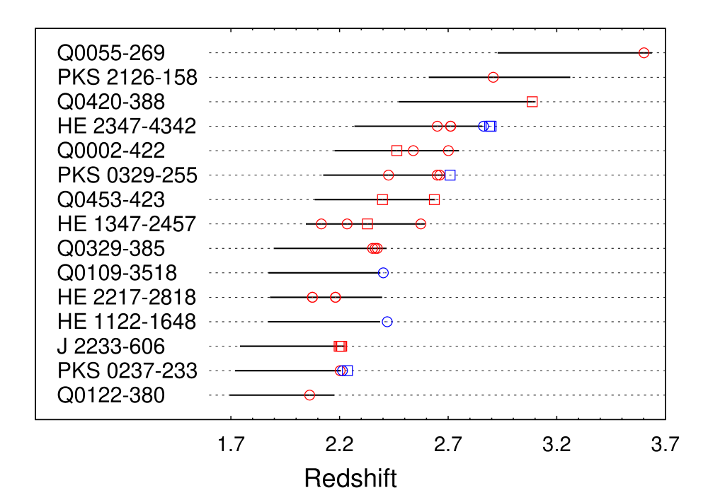
Figure 4.1: Schematic diagram showing the positions of the intervening (red) and associated (blue) absorbers in redshift space along the lines of sight of the sampled QSOs. The multiplicity of the system is denoted by different symbols: up to 3 components (circles) and more than 3 components (squares). The solid horizontal lines indicate redshift coverage $[z_{\rm min},\leavevmode\nobreak\ z_{\rm max}]$ along each line of sight (dotted).

The total probed redshift path in our sample is $\Delta z=8.34$, in the range $2.06\leq z\leq 2.91$. The corresponding redshift-invariant absorption path length (also called ‘absorption distance’) can be calculated by solving the following integral:

$$X=\int\limits_{z_{\rm min}}^{z_{\rm max}}\frac{(1+z)^{2}}{\sqrt{{\Omega_{m}}(1+z)^{3}+\Omega_{\Lambda}}}dz.$$ (4.1)

The absorption path length for each QSO is specified in Appendix A, Table  LABEL:observed_quasars (column 4). By summing up the path lengths at each sightline, we obtain a total absorption path length for the whole O vi sample $\sum\limits_{i}X_{i}=\Delta X=27.3$.

To minimize the uncertainties in determination of column densities and Doppler parameters we imposed strict selection criteria when composing the final O vi sample, removing those systems that are heavily blended by other intergalactic lines. This means, however, that the rate of incidence $d\mathcal{N}/dz$ (the number of absorbers per redshift path length interval) is underestimated when using these strict selection criteria for the analysis of the O vi line density. Therefore, we added other 11 intervening O vi systems from the original (unrestricted) sample, only for the determination of $d\mathcal{N}/dz$ and $d\mathcal{N}/dX$. In these 11 systems, both O vi lines are clearly detected, but partly blended, so that these systems can be used only to constrain the O vi incidence rate, but not the physical conditions in the O vi systems.

The calculated rate of incidence for the extended sample of 43 intervening O vi systems is $d\mathcal{N}/dz=5.2\pm 0.79$. This estimate was obtained by probing the full range of column densities ($11.5\leq\log N\leq 15.5$), while the proximity zones of $\leq$ 5000 km s^-1 for each line of sight were excluded. The corresponding rate of incidence per absorption path length is $d\mathcal{N}/dX=1.6\pm 0.24$. For comparison, Muzahid et al. (2012) found $d\mathcal{N}/dz=10.1\pm 1.15$ and $d\mathcal{N}/dX=3.1\pm 0.35$, respectively; i.e., roughly twice higher values, using similar data and a similar redshift range. However, their sample includes some systems where one of the O vi lines is blended by saturated Ly-$\alpha$ or both O vi and dubious absorption features that might not be at all associated with intervening O vi . Therefore, our estimate of the rate of incidence might be considered as a lower limit, while the one by Muzahid et al. (2012) – as an upper limit.

Table 4.1: Number of components in the intervening and associated O vi systems with or without O vi -H i alignment.

Systems
Type	Total	Intervening systems		Associated systems
		O vi ​​/H i al.	No al.	O vi ​​/H i al.	No al.
1 comp.	10	6	3	1	0
2-3 comp.	18	7	7	3	1
multicomp.	12	4	5	0	3

An important characteristic parameter of intervening absorption-line systems is the number of absorption components (i.e., velocity components) per system. Detailed information on the number of components in each studied O vi system is presented in Table LABEL:observed_quasars, column 7. The results are summarized in Table 4.1. Two subsamples can be distinguished: (1) absorbers with at least one O vi component aligned in velocity space with H i within 10 km s^-1 ​​, and (2) absorbers without any such alignment. Fig. 4.2 (top panel) displays the distribution of O vi intervening systems, according to the number of their components and to their alignment with H i ​​. Evidently, one third of the components in the single-component systems do not exhibit alignment with H i while this fraction grows to 50 per cent in two-three component systems. The tendency persists as well in the multicomponent case where systems without alignment slightly dominate. The existence of alignment between O vi and H i is important for the performed ionization modeling, as demonstrated later in this Chapter (Sect. 4.3). Lack of alignment indicates that the O vi and H i absorption arise in physically distinct regions and gas phases.

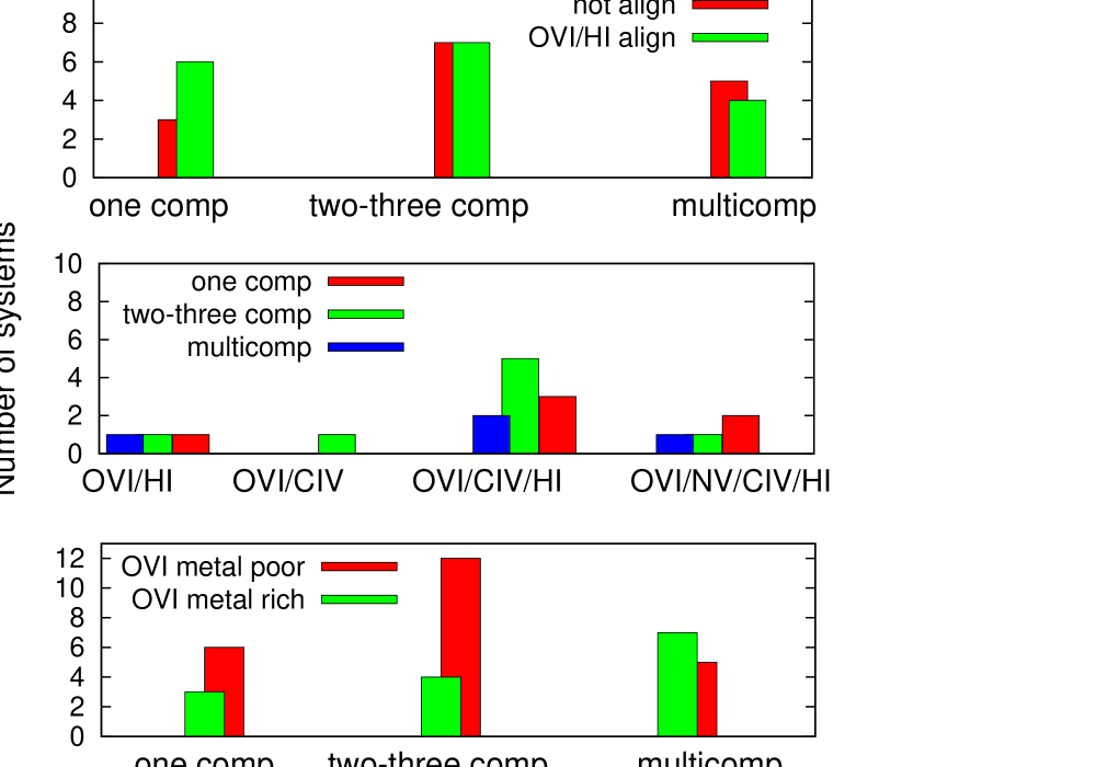
Figure 4.2: Statistics of the O vi absorbers from the UVES sample: (top panel) Fraction of absorbers with at least one O vi component aligned with H i (within 10 km s^-1 ​​) in the single-, two-three and multicomponent sample; (middle panel) Number of O vi systems aligned with C iv ​​, N v and/or H i ; (bottom panel) Statistics of the considered O vi systems according to the number of components.

A component alignment in velocity space between O vi and other metal lines such as C iv is another characteristic of the absorbers that deserves special attention, because the combined use of ions with different ionization potentials provide important constraints for the photoionization modeling. Thirty-three O vi systems (27 intervening and 6 associated) out of 40 in our sample exhibit C iv absorption and 11 of them (9 intervening and 2 associated) show N v absorption. Fifteen C iv ​​/O vi pairs in the intervening systems are aligned (i.e. their component velocity offsets are within 10 km s^-1 ​​). The statistics on O vi absorbers aligned with C iv ​​, N v and/or H i lines according to the number of their components is shown in Fig. 4.2 (middle panel). It appears that alignment between the components of the three ions C iv ​​, N v ​​, and O vi occurs most frequently in systems with one to three absorption components (one fourth of this subsample).

4.2 Key observables

4.2.1 Metal-rich and metal-poor O vi absorbers

As already mentioned in Sect. 3.3, Bergeron & Herbert-Fort (2005) suggested a classification of O vi absorbers in two populations: metal-rich absorbers (“type 1”; $N(\mbox{O\,{\sc vi}\leavevmode\nobreak\ }\!\!)/N(\mbox{H\,{\sc i}\leavevmode\nobreak\ }\!\!)\\ >0.25$) and metal-poor (“type 0”; $N(\mbox{O\,{\sc vi}\leavevmode\nobreak\ }\!\!)/N(\mbox{H\,{\sc i}\leavevmode\nobreak\ }\!\!)<0.25$). We follow their approach to investigate the physical reasoning behind this distinction and independently study the distributions of Doppler parameter and column density for both absorber classes. The total O vi and H i column densities of the sampled systems are defined as the sums of the column densities of their components. The extremal values of the ratio are estimated as follows:

$$\sigma^{\rm max}_{\rm ratio}=\frac{N(O\,\text{\sc vi})_{\rm tot}+\sigma^{+}(N(O\,\text{\sc vi}))_{\rm tot}}{N(H\,\text{\sc i})_{\rm tot}-\sigma^{-}(N(H\,\text{\sc i}))_{\rm tot}}-\frac{N(O\,\text{\sc vi})_{\rm tot}}{N(H\,\text{\sc i})_{\rm tot}},$$

$$\sigma^{\rm min}_{\rm ratio}=\frac{N(O\,\text{\sc vi})_{\rm tot}}{N(H\,\text{\sc i})_{\rm tot}}-\frac{(N(O\,\text{\sc vi})_{\rm tot}-\sigma^{-}(N(O\,\text{\sc vi}))_{\rm tot}}{(N(H\,\text{\sc i})_{\rm tot}+\sigma^{+}(N(H\,\text{\sc i}))_{\rm tot}}.$$

The results and the estimated $1\sigma$ deviations $\sigma^{\pm}$ are presented in Appendix A, Table LABEL:column_density_ratio and A.3, respectively.

In Fig. 4.2 (bottom panel) is shown the distribution of metal-rich and metal-poor systems, according to the number of their components. Evidently, most of the metal-poor absorbers ($\approx$ 79 per cent) inhabit in systems with one to three components, whereas the metal-rich systems (about one third of the whole sample) tend to be more dispersed in the component space.

4.2.2 Distributions of Doppler parameter and column density

In this section we present briefly the obtained Doppler parameter and column density distributions of the observed O vi absorbers. (More detailed analysis and comparison with the results from OWLS are provided in Sect. 5.1.2.) The distributions of the whole UVES sample are shown in Fig. 4.3. The median value for the Doppler parameter is 13.0 km s^-1 ​​, which corresponds to $T_{\rm UVES}\sim 1.6\times 10^{5}$ K, assuming purely thermal broadening. This temperature is consistent with the result of Muzahid et al. (2012): $T\sim 1.8\times 10^{5}$  K, obtained from a similar UVES data set.

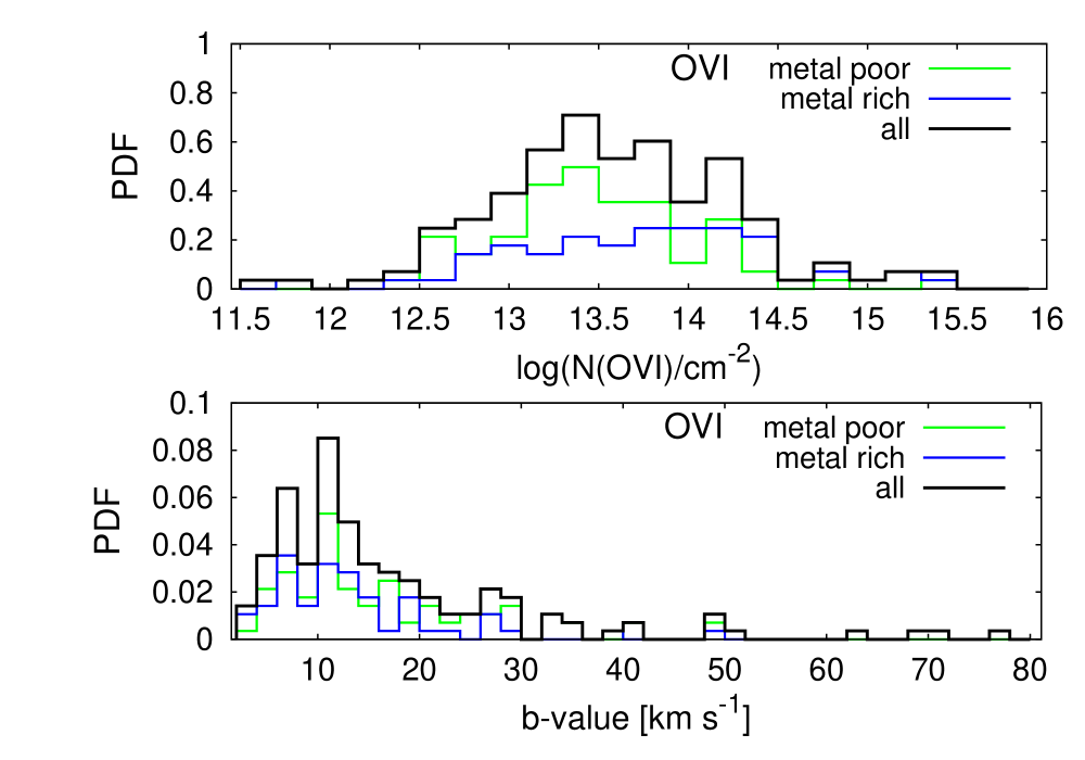
Figure 4.3: Column density (top) and Doppler parameter (bottom) distributions for all (black), metal-rich (blue) and metal-poor (green) O vi components.

The fractional column density and Doppler-parameter distributions for the populations of metal-rich and metal-poor absorbers are compared in Fig. 4.3. No significant difference between the fractional $b$ distributions is seen. In contrast, the column density distributions appear to be different. The distribution peaks at log N(O vi ​​)$\approx 14.0$ for metal-rich systems, whereas the column densities of their metal-poor peers span a narrower range, centered at log N(O vi ​​)$\approx 13.4$. The latter value is close to the median of the total sample: log N(O vi ​​)$\approx 13.6$.

The column density distribution function

The column density distribution function (CDDF), $f(\text{O\,{\sc vi}})$, is defined as the number of absorption systems ${\mathcal{N}}(N_{\text{O\,{\sc vi}}})$ per column density bin $\Delta N_{\text{O\,{\sc vi}}}$ and per unit absorption path length $\Delta X$ (Petitjean et al., 1993):

$$f(N_{\text{O\,{\sc vi}}})=\frac{\mathcal{N}}{\Delta N_{\text{O\,{\sc vi}}}\times\sum\limits_{i=1}^{n}X_{i}},$$ (4.2)

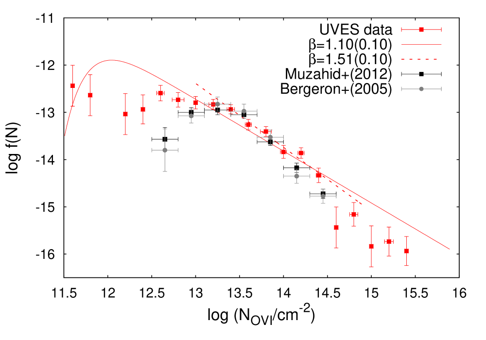
Figure 4.4: CDDF from the UVES sample, fitted with power law functions: corrected for completeness (solid line) and with lower threshold $N(\rm\mbox{O\,{\sc vi}\leavevmode\nobreak\ })\approx 13.3$ (dashed). The data points obtained by Muzahid et al. (2012) and by Bergeron & Herbert-Fort (2005) are plotted for comparison.

From the total absorption path length, obtained in Sect. 4.1, we derive the CDDF from the UVES data. The result is plotted in Fig. 4.4. The uncertainties on the $Y$ axis are estimated by the Poisson noise of the CDDF values while those on the $X$ axis, $\sigma(N_{\footnotesize\rm\mbox{O\,{\sc vi}\leavevmode\nobreak\ }\!\!})$, are calculated as follows:

• Each column density value in a given bin is taken with a weight $\omega_{i}$ which reflects the fitting error $\sigma_{i}$:

  $$\omega_{i}=1/\sigma_{i}^{2}$$

• The weighted mean for each bin is calculated from the column densities $N_{i}$ that fall within it:

  $$N_{\text{bin}}=\frac{\displaystyle{\sum_{i}\omega_{i}N_{i}}}{\displaystyle{\sum_{i}\omega_{i}}},$$

• Finally, the dispersion $D(N_{\text{bin}})$, is obtained from:

  $$D(N_{\text{bin}})=\sigma(N_{\text{bin}})=\sqrt{<N_{i}-N_{\text{bin}}>^{2}},$$

  where

  $${<N_{i}-N_{\text{bin}}>}^{2}=\frac{\displaystyle{\sum_{i}\omega_{i}(N_{i}-N_{\text{bin}})^{2}}}{\displaystyle{\sum_{i}\omega_{i}}}.$$

The data were fitted with a single power-law and with a power-law, multiplied by a completeness function (Fig. 4.4, dashed and solid lines). In the second case we followed the procedure of Ben Bekhti et al. (2012):

• Calculation of the signal-to-noise (S/N) ratio. For normalized spectra and per resolution element, it can be computed through:

  $$\text{S/N}=\sqrt{\frac{\Delta\lambda_{r}}{\Delta\lambda_{p}}}\frac{1}{\sigma_{p}^{\rm RMS}}\leavevmode\nobreak\ ,$$

  where $\Delta\lambda_{r}$ and $\Delta\lambda_{p}$ are the wavelength separations per resolution and per pixel element and ${\sigma_{p}^{\rm RMS}}$. We calculated the S/N ratio for 36 out of 40 O vi systems with UVES spectra. It was not possible to estimate $\sigma_{p}^{\rm RMS}$ and the S/N ratio for 4 systems. In three cases, two nearby systems turned out to have identical S/N ratio.

  The S/N ratio was calculated as well for C iv and H i systems. The S/N distribution for spectral bands around the O vi ​​, C iv and H i lines is shown in Fig. 4.5.

  

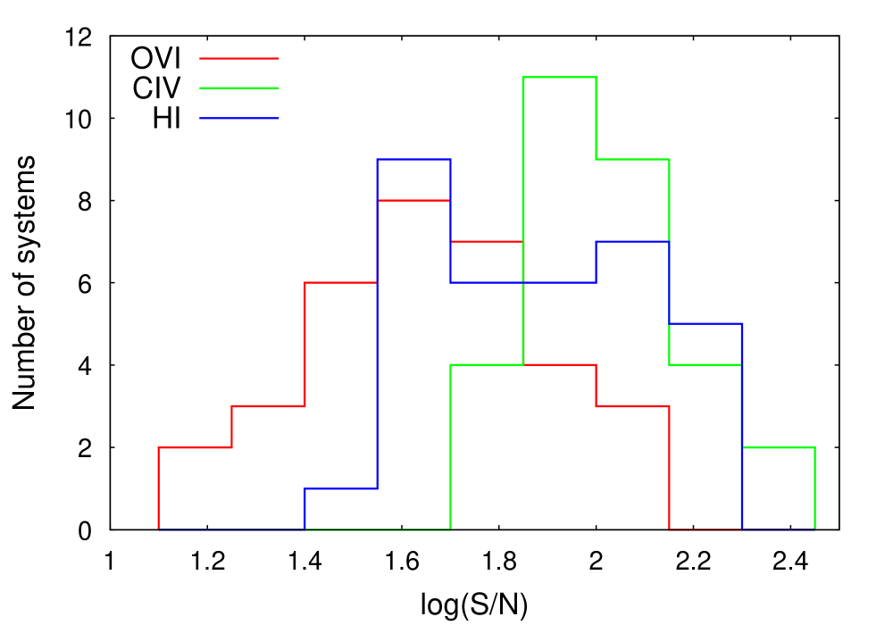
  Figure 4.5: Distribution of S/N for the studied O vi absorbers (red), compared to those for C iv and H i systems (green and blue, respectively).

• Calculation of the column density detection limit for all 36 O vi systems: the 3$\sigma$ limiting equivalent width of an unresolved line at wavelength $\lambda_{0}$ (see Tumlinson et al. (2002), their Eq. 1) is given by:

  $$W_{\lambda,\text{limit}}=\frac{\sigma\lambda_{0}}{(\lambda/\Delta\lambda)\text{(S/N)}},$$

  where $\lambda/\Delta\lambda$ is the spectral resolution. The relation between the equivalent width and the column density for small optical depths ($\tau\ll 1$) is linear (see Eq. 2.35).

  Replacing $W_{\lambda}$ from Eq. 2.35 with $W_{\lambda,\text{limit}}$, one can estimate the column density detection limit $N_{\text{limit}}$:

  $$N_{i,\text{limit}} = \frac{{\rm m_{e}}c^{2}}{\pi\rm e^{2}}\frac{\sigma}{(\lambda/\Delta\lambda)\text{(S/N)}f_{ij}\lambda_{0}}$$

  $$= 1.13\times 10^{20}\frac{\sigma}{\frac{\lambda}{\Delta\lambda}\big{(}\frac{\rm S}{\rm N}\big{)}f_{ij}\frac{\lambda_{0}}{\AA}}\leavevmode\nobreak\ \leavevmode\nobreak\ \leavevmode\nobreak\ \leavevmode\nobreak\ \leavevmode\nobreak\ \leavevmode\nobreak\ \leavevmode\nobreak\ \leavevmode\nobreak\ \leavevmode\nobreak\ \leavevmode\nobreak\ \leavevmode\nobreak\ \leavevmode\nobreak\ \leavevmode\nobreak\ \leavevmode\nobreak\ \leavevmode\nobreak\ \leavevmode\nobreak\ \leavevmode\nobreak\ \rm[cm^{-2}].$$

  Taking into account the UVES spectral resolution $(\lambda/\Delta\lambda)=45\,000$ and adopting a $3\sigma$ threshold level (i.e., $\sigma=3$), we calculated $N_{i,\text{limit}}$ for O vi ​​, C iv and H i absorption in the sampled 36 systems. The cumulative normalized distribution of O vi ​​, C iv and H i absorbers per column density bin, when certain $N_{i,\text{limit}}$ thresholds are imposed, is shown in Fig. 4.6.

  

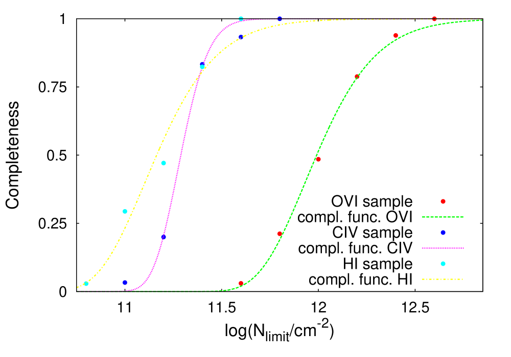
  Figure 4.6: Column-density completeness of the UVES sample.

• Fitting of CDDF by use of an error function: following Ben Bekhti et al. (2012), we introduce the parametrized error function:

  $$C(\text{log}N_{i,\text{limit}};a,b)=\frac{1}{2}\text{erf}[a(\text{log}(N_{i,\text{limit}}-b))]+\frac{1}{2}.$$

  This function can be understood as a completeness function, as it returns the fraction of sightlines which potentially can reveal an absorber with column density $N_{i,\text{limit}}$. The parameter $a$ describes the shape of the function and the parameter $b$ accounts for the offset.

  Fig. 4.4 demonstrates that the CDDF drops at lower column densities due to the increasing incompleteness of the sample. To describe this behavior the completeness function $C$ is incorporated into the CDDF-fitting function:

  $$f(\text{log}N_{i})=\beta\text{log}N_{i}+n+\text{log}C(\text{log}N_{i};a,b),$$

  where $\beta$ is the slope of the power-law part and $n$ is a normalization constant. The shape parameter $a$ is fixed to a constant value as determined from the curves in Fig. 4.6 and varied only the offset $b$ of the completeness function.

The obtained slope of the fitted completeness function for the full range of column densities is $\beta\approx 1.10\pm 0.10$. It changes sensibly up to $\beta\approx 1.51\pm 0.10$ when the data are fitted by a single power-law function (without completeness corrections) and an apparent threshold of log$N(\rm\mbox{O\,{\sc vi}\leavevmode\nobreak\ }\!\!)\approx 13.3$ is imposed as a lower limit. Obviously the slope is very sensitive to the choice of a threshold. Next, we compare in Fig. 4.4 our results of CDDF with this derived by Bergeron & Herbert-Fort (2005) (gray) and Muzahid et al. (2012) (black) from the same sample of UVES data. In both works a steeper slope is obtained; e.g. $\beta=1.71\pm 0.48$ (Bergeron & Herbert-Fort, 2005). However, within the uncertainties, all derived distributions are in a good agreement in the column density range $13.3\leq\log N(\rm\mbox{O\,{\sc vi}\leavevmode\nobreak\ }\!\!)\leq 14.3$. Neither Bergeron & Herbert-Fort (2005) nor Muzahid et al. (2012) find any components with column densities higher than $\log N(\rm\mbox{O\,{\sc vi}\leavevmode\nobreak\ }\!\!)\approx 14.5$. Components with such values in our study originate from four multicomponent systems that include other species, such as C iv and N v ​​. They are found along two sightlines: HE 2347-432 and J 2233-606. The latter QSO is not included in the sample of Muzahid et al. (2012). Three of these systems turn out to be saturated (HE 2347-432 at $z=2.897458$, HE 2347-432 at $z=2.891062$, and J 2233-606 at $z=2.198231$) which leads to large uncertainties for the determination of $N$. The fourth system J 2233-606 at $z=2.204508$ is not saturated, but blended. On the other hand, the two bins of lowest column density in our sample include only one component each (see Fig. 4.4). These components are part of the systems HE 2347-432 at $z=2.897458$ and HE 2347-432 at $z=2.891062$, respectively. Muzahid et al. (2012) do not include them in the sample used for derivation of the CDDF.

4.2.3 Contribution to cosmic baryon density

The contribution of the O vi absorbers to the cosmic baryon density, $\Omega_{\footnotesize\rm\mbox{O\,{\sc vi}\leavevmode\nobreak\ }}$, can be estimated through the formula:

$$\Omega_{{\footnotesize\rm\mbox{O\,{\sc vi}\leavevmode\nobreak\ }}}=\frac{1}{\rho_{c}}m_{{\footnotesize\rm\mbox{O\,{\sc vi}\leavevmode\nobreak\ }}}\frac{\Sigma\leavevmode\nobreak\ w_{i}\leavevmode\nobreak\ N_{{\footnotesize\rm\mbox{O\,{\sc vi}\leavevmode\nobreak\ }\!\!},i}}{(c/H_{0})\Sigma\leavevmode\nobreak\ \Delta X},$$ (4.3)

where $\rho_{c}$ is the critical density, $m_{\footnotesize\rm\mbox{O\,{\sc vi}\leavevmode\nobreak\ }\!\!}$ is the mass of the oxygen atom, $\Delta X$ is the absorption path length (see Eq. 4.1), $w_{i}$ is the completeness correction as calculated in the previous subsection (see Fig. 4.6), and $N_{{\footnotesize\rm\mbox{O\,{\sc vi}\leavevmode\nobreak\ }\!\!},i}$ are column densities of the individual absorbers (Burles & Tytler, 1996). Here, the value of the Hubble constant is taken to be: $H_{\rm 0}=73$ km s^-1 ​​Mpc.

To achieve a statistically significant result, we calculate the cosmic density of O vi ​​ absorbers from the extended sample of 43 intervening systems in the redshift range $2.04\leq z\leq 3.60$. The obtained estimate is $\Omega_{{\footnotesize\rm\mbox{O\,{\sc vi}\leavevmode\nobreak\ }\!\!}}=3.3\times 10^{-7}$, for the full column density range $11.5\leq\log N\leq 15.5$. For comparison, the result of Bergeron & Herbert-Fort (2005) is a factor of 2 less: $\Omega_{{\footnotesize\rm\mbox{O\,{\sc vi}\leavevmode\nobreak\ }\!\!}}=1.5\times 10^{-7}$, while Muzahid et al. (2012) obtain an even lower value of $\Omega_{{\footnotesize\rm\mbox{O\,{\sc vi}\leavevmode\nobreak\ }\!\!}}=1.0\times 10^{-7}$, with a lower column density cutoff of 13.7 in log scale.

The cosmological density of baryons, associated with the O vi absorbing phase, can be estimated by use of a similar formula:

$$\Omega^{{\footnotesize\rm\mbox{O\,{\sc vi}\leavevmode\nobreak\ }}}_{{\tiny\rm IGM}}=\frac{1}{\rho_{c}}\mu m_{{\tiny\rm H}}\frac{\Sigma\leavevmode\nobreak\ w_{i}\leavevmode\nobreak\ N_{{\footnotesize\rm\mbox{O\,{\sc vi}\leavevmode\nobreak\ }\!\!},i}}{(c/H_{0})(f_{{\footnotesize\rm\mbox{O\,{\sc vi}\leavevmode\nobreak\ }}}Z(\rm O/\rm H)_{\odot})\Sigma\leavevmode\nobreak\ \Delta X},$$ (4.4)

where the mean atomic weight is taken to be $\mu=1.3$, $m_{\rm H}$ is the mass of the hydrogen atom, $f_{\footnotesize\rm\mbox{O\,{\sc vi}\leavevmode\nobreak\ }}$ is the ionization fraction of O vi , and $Z$ is the gas metallicity (Tripp et al., 2000). Following Muzahid et al. (2012), we adopt $f_{\footnotesize\rm\mbox{O\,{\sc vi}\leavevmode\nobreak\ }\!\!}=0.2$ and $Z=0.1Z_{\odot}$ and obtain $\Omega^{{\footnotesize\rm\mbox{O\,{\sc vi}\leavevmode\nobreak\ }\!\!}}_{{\rm IGM}}/\Omega_{\rm b}=0.00856$ with $\Omega_{\rm b}=0.0418$ (Spergel et al., 2007). The fraction of baryons associated with O vi absorbers turns out to be less than 1 per cent of the total baryon density. This value – as we shall see later – is in excellent agreement with the predictions from the cosmological simulations (Sect. 5.4). For comparison, Muzahid et al. (2012) find a slightly higher value. According to their estimate, the contribution of the O vi absorbers to the total baryon density in the Universe is 2.8 per cent.

4.2.4 Velocity widths and velocity offsets

We investigated the velocity widths (or spreads) of the O vi absorbers in our UVES sample and their velocity offsets to the corresponding H i and C iv lines. The weighted mean velocity for a given spectral profile is defined as:

$$\langle v_{\rm w}\rangle=\frac{\displaystyle{\sum_{v_{\rm min}\leq v_{i}\leq{v_{\rm max}}}v_{i}(F_{c}-F_{i}})}{\displaystyle{\sum_{v_{\rm min}\leq v_{i}\leq{v_{\rm max}}}(F_{c}-F_{i})}}\leavevmode\nobreak\ ,$$ (4.5)

where $F_{c}\equiv 1$ is the continuum flux, $F_{i}$ is the normalized flux per pixel, $v_{i}$ is the velocity per pixel and $v_{\rm min}$ and $v_{\rm max}$ are the velocities corresponding to the lower and upper limit (or left and right absorption sides) of the fitting Voigt profile ($F(v_{\rm min})=F(v_{\rm max})=F_{c}$). The absorption-velocity spread $\delta v$ is calculated simply as $[v_{\rm max}-v_{\rm min}]$ which is a good first-order approximation of this quantity when the line wings are not very wide (Ledoux et al., 2006).

The velocity spreads and the weighted mean velocities for each O vi ​​, C iv and H i ​​ absorption feature were calculated in 34 out of 40 considered O vi systems. Six O vi systems were excluded from the sample due to a very high uncertainty of $\langle v_{\rm w}\rangle$. Table LABEL:fig_velocity_spread (Appendix A.5) lists lower, $v_{\rm min}$, and upper, $v_{\rm max}$, velocity limits (or left and right sides of the absorption feature) for the species O vi ​​, C iv ​​, N v and H i ​​, where the velocity zero point $v=0$ is set at the center of the strongest O vi line. The O vi and H i velocity spreads for each absorber are also given. In some cases, two different sets $(v_{\rm min},\leavevmode\nobreak\ v_{\rm max},\leavevmode\nobreak\ \delta v)$ are calculated: one for the associated O vi absorber and a second one that characterizes the system itself.

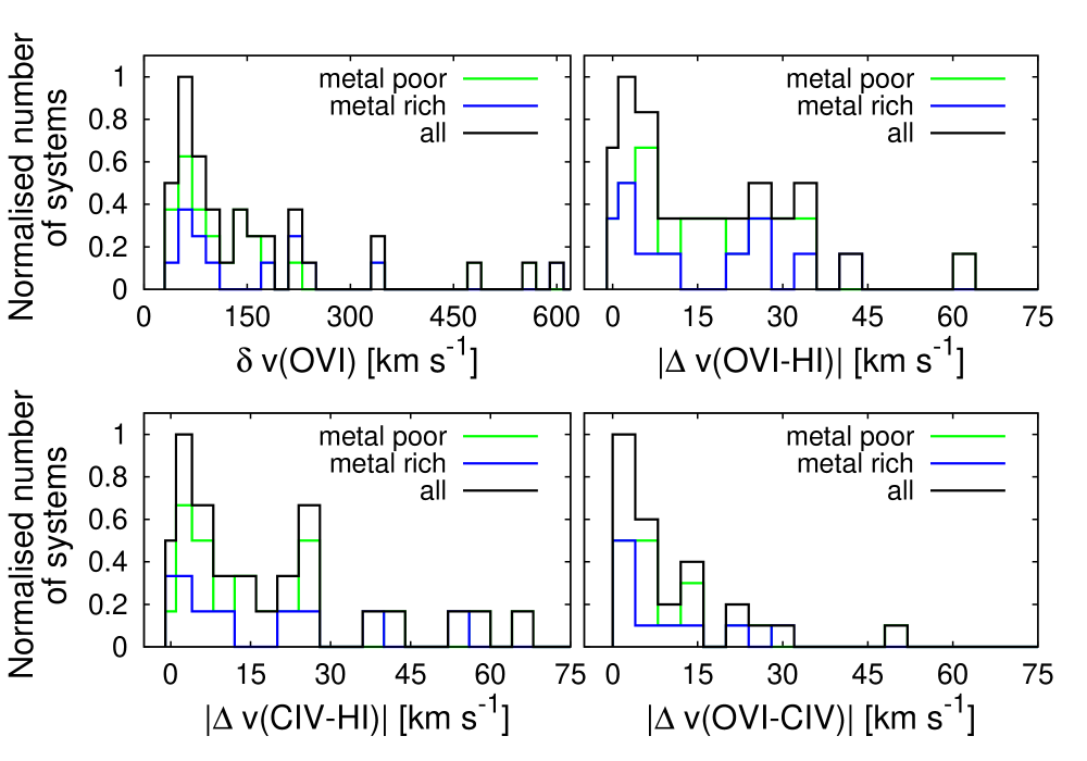
Figure 4.7: Distributions of O vi velocity spread (top left panel) and of the velocity offsets between the absorption features O vi -H i (top right panel), C iv -H i (bottom left panel) and O vi -C iv (bottom right panel).

The distribution of the O vi velocity spread for metal-rich and metal-poor absorbers is plotted in Fig. 4.7 (top left panel). Evidently, there is a clear maximum at about 40 km s^-1 ​​. The large spread in the distribution indicates the complex kinematics of spatially separated metal-enriched gas phases in the absorbing gas structures.

Then the velocity offset $\Delta v$ between O vi ​​, C iv and H i absorbers was obtained through:

$$\lvert\Delta v(\text{X}_{1}-\text{X}_{2})\rvert=\lvert\langle{v_{\rm w}(\text{X}_{1})}\rangle-\langle{v_{\rm w}(\text{X}_{2})}\rangle\rvert\leavevmode\nobreak\ ,$$

where $\text{X}_{1}$ and $\text{X}_{2}$ are the studied species (ions). The normalized distributions of the velocity offsets between O vi ​​, C iv and H i weighted mean velocities are shown in Fig. 4.7. In all considered cases, the systems were classified as metal-rich or metal-poor, according to the criterion of Bergeron & Herbert-Fort (2005) (see Sect. 3.3). The distributions of the velocity offsets $\Delta v(\text{O\,{\sc vi} - H\,{\sc i}})$ (top right panel) and $\Delta v(\text{C\,{\sc iv} - H\,{\sc i}})$ (bottom left panel) are evidently bimodal, while the distribution of the velocity offset $\Delta v(\text{O\,{\sc vi} - C\,{\sc iv}})$ (bottom right panel) is not. Looking for some specific characteristics that might be related to this bimodality, we delineated two subsamples with velocity offsets in ranges $\sim 10-20\leavevmode\nobreak\ \rm km\leavevmode\nobreak\ s^{-1}$ around the peaks: $\lvert\Delta v_{\rm min}(\text{O\,{\sc vi} - H\,{\sc i}})\rvert=[0-13]\leavevmode\nobreak\ \rm km\leavevmode\nobreak\ s^{-1}$, $\lvert\Delta v_{\rm max}(\text{O\,{\sc vi} - H\,{\sc i}})\rvert=[22-38]\leavevmode\nobreak\ \rm km\leavevmode\nobreak\ s^{-1}$, and $\lvert\Delta v_{\rm min}(\text{C\,{\sc iv}}-\text{H\,{\sc i}})\rvert=[0-12]\leavevmode\nobreak\ \rm km\leavevmode\nobreak\ s^{-1}$, $\lvert\Delta v_{\rm max}(\text{C\,{\sc iv}}-\text{H\,{\sc i}})\rvert=[20-30]\leavevmode\nobreak\ \rm km\leavevmode\nobreak\ s^{-1}$, respectively.

A characteristic of the absorbers which seems to be related to the bimodality of the $\lvert\Delta v(\text{O\,{\sc vi}}-\text{H\,{\sc i}})\rvert$ distribution is the number of components in a given system. As seen in Fig. 4.8, top panel, the majority of objects within range of the first peak (13 out of 17) exhibit a simple structure with 1 up to 3 absorption components. The population around the second peak range is apparently different: 7 out of 12 systems are multicomponent and have a more complex structure.

This trend implies that absorbers with small velocity offsets between O vi and H i (i.e., absorbers within range of the first peak) represent kinematically simple, isolated gas structures. O vi absorbers that have a significant velocity offset compared to H i instead appear to be embedded in a kinematically more complex host structure with a larger internal velocity dispersion, as expected, for instance, for gaseous material expelled from galactic winds and outflows.

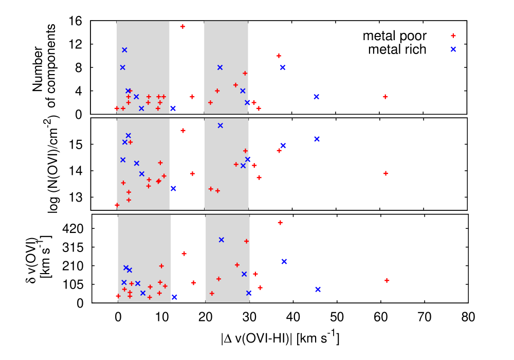
Figure 4.8: Diagram O vi -H i velocity offset vs. number of components (top panel), column density (middle panel) and absorption width (bottom panel) in a given O vi system. Zones of peaks in the velocity offset distributions (shadowed areas) are shown.

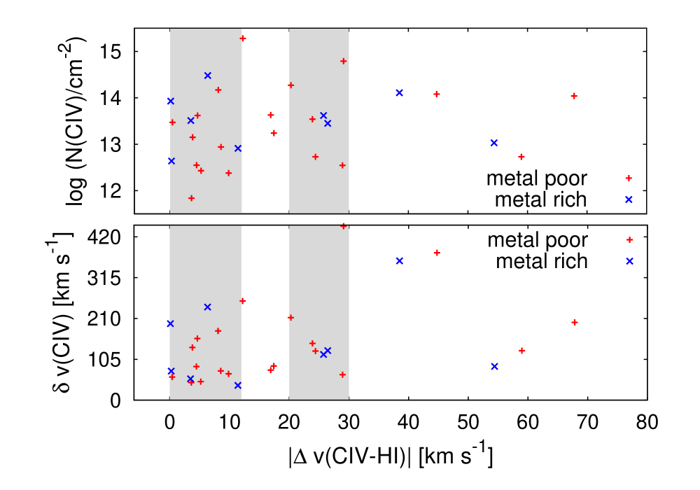
Figure 4.9: Velocity offset between the weighted mean velocities of C iv and H i absorption features versus C iv absorption width (bottom panel) and C iv column density (top panel). Zones of peaks in the velocity offset distributions (shadowed areas) are shown.

Other properties of O vi ​​, C iv and H i absorption features, that can be studied in relation to the evident bimodality of the velocity offset distributions, are the velocity spreads and the total column density. Although the interpretation of the observed trends for these quantities is not straight-forward, we nevertheless discuss their properties to gain an insight into the kinematics of the absorbing gas structures. Our tests are performed and illustrated in Figs. 4.8, middle and bottom panels, and 4.9, respectively. In both cases, the zone of the low velocity offset seem to be populated mainly by metal-poor systems.

Weak correlations between the velocity width, the column density and the velocity offset are seen in Fig. 4.8: systems with $\lvert\Delta v(\text{O\,{\sc vi}}-\text{H\,{\sc i}})\rvert\leq 13\leavevmode\nobreak\ \rm km\leavevmode\nobreak\ s^{-1}$ are mostly systems with low velocity spread $\delta v(\text{O\,{\sc vi}})\leq 105\leavevmode\nobreak\ \rm km\leavevmode\nobreak\ s^{-1}$. On the other hand, O vi systems with velocity offsets in the range of the second peak ($\lvert\Delta v(\text{O\,{\sc vi}}-\text{H\,{\sc i}})\rvert\geq 22\leavevmode\nobreak\ \rm km\leavevmode\nobreak\ s^{-1}$) are mostly systems of higher column density $\log N$(O vi)$\geq 14$. A similar correlation is found as well considering the H i absorption in those systems. Among the systems from the subsample with low velocity offsets, 82 per cent exhibit column densities $\log N(\text{H\,{\sc i}})\leq 14.9$ while systems with high velocity offsets are typically objects with high column density: 75 per cent of them have $N(\text{H\,{\sc i}})\geq 15.0$.

The same tendency concerning the H i column density is evident when $\lvert\Delta v(\text{C\,{\sc iv}}-\text{H\,{\sc i}})\rvert$ is considered: 73 per cent of the absorbers in the first subsample have $\log N(\text{H\,{\sc i}})\leq 14.9$ vs. $\log N(\text{H\,{\sc i}})\geq 14.9$ for 80 per cent of the absorbers in the one with high velocity offsets.

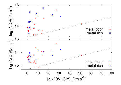
Figure 4.10: Velocity offset between the weighted mean velocities of O vi and C iv absorption features versus column density of C iv (bottom panel) an O vi (top panel). The possible presence of a lower envelope is indicated by black line.

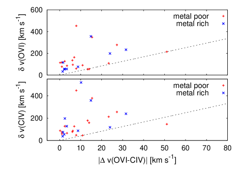
Figure 4.11: Velocity offset between the weighted mean velocities of O vi and C iv absorption features versus velocity spread of C iv (bottom panel) and O vi (top panel). The possible presence of a lower envelope is indicated by the black line.

Finally we study the possible relation of velocity offsets between O vi and C iv ​​ absorption features and the corresponding column densities $N$(X) and velocity widths $\delta v(\text{X})$ (Figs. 4.10 and 4.11). It seems that metal-poor systems have preferably lower column densities: $\log N$(O vi)$\leq$14 (Fig. 4.10, upper panel). Most of the systems are characterized by low velocity offset: $\lvert\Delta v(\text{O\,{\sc vi}}-\text{C\,{\sc iv}})\rvert\leq 20\leavevmode\nobreak\ \rm km\leavevmode\nobreak\ s^{-1}$. Systems with higher O vi - C iv velocity offset are those with higher column density ($\log N$(O vi)$\geq 14$) and velocity spread $\delta v(\text{O\,{\sc vi}})\geq 100\leavevmode\nobreak\ \rm km\leavevmode\nobreak\ s^{-1}$ (Figs. 4.10 and 4.11, upper panels). A similar trend is observed when the velocity spread of C iv is considered (Fig. 4.11, lower panel). These findings are consistent with the study of Muzahid et al. (2012).

4.3 Ionization modeling with Cloudy

As shown in the previous section, only a fraction of the O vi absorbers in our sample is kinematically aligned with H i and C iv ​​. Only for such aligned systems it is reasonable to assume that the above ions trace the same physical regions within the host structure and that an ionization model provides meaningful results.

To investigate the physical conditions in kinematically aligned O vi ​​/H i absorbers, we modeled the ion column densities of selected absorbers from the UVES sample using the photoionization code Cloudy (version C08; Ferland et al., 1998). For this, we follow a strategy that is similar to that adopted for the case study of 2 individual absorbers presented in Sect. 3.2. A solar abundance pattern of O and C was assumed. We adopt an optically thin plane-parallel geometry of systems in photoionization equilibrium exposed to a Haardt & Madau (2001) UV background spectrum at $z=2.16$, normalized to $\log\leavevmode\nobreak\ J_{912}=-21.15$ (Scott et al., 2000) at the Lyman limit.

The number of O vi ​​/H i pairs aligned in velocity space ($\Delta v_{\rm comp.}\leq$ 10 km s^-1 ​​) is given in Table 4.1. We modeled 6 single-component intervening systems, 7 intervening systems with $2-3$ absorption components, 4 intervening milticomponent systems and 1 intervening system with 3 components and a velocity shift of $\approx$11 km s^-1 ​​. Five associated O vi systems with up to 3 components were also modeled as a test sample. The models in the latter case give limits of the output physical parameters, since only an UV background spectrum (Haardt & Madau, 2001) was included as input spectrum without taking into account the effect of the local quasar spectrum. Details on each model are specified in Appendix B.

We consider the following input model parameters:

• Measured column densities of C iii and/or C iv ​​, when present;

• Column density of O vi ​​;

• Metallicity $Z$ (in solar units);

• Hydrogen volume density $n_{\rm H}$.

The parameter ranges for the metallicity and hydrogen density were $0.001\leq\leavevmode\nobreak\ Z/Z_{\odot}\leq 1$ and $-5\leq\,$log$\leavevmode\nobreak\ n_{\rm H}\leq 0$, respectively. In some cases, we derive super-solar metallicities together with very low corresponding volume densities. We included this results in the tables as possible solutions of Cloudy, although the physical meaning remains unclear. The column density of the H i component that is closest to the modeled O vi has been taken directly from observations as a stopping criterion for modeling. In two individual cases, PKS 0237-233 at $z=2.202783$ and Q 0453-423 at $z=2.636236$, Si iii and Si iv were modeled as well.

The first step in the modeling procedure was to derive models using Cloudy for a discrete set of values of $Z$ and $n_{\rm H}$. In case that C iii and/or C iv were present, the output column densities $N$(C iii ​​), $N$(C iv ​​) and $N$(O vi ​​) were compared to the observed ones. The input parameters $Z$ and $n_{H}$ then were adjusted before the next iteration step, until the differences between the output column densities and the observed values became negligible. Thus an unique solution was obtained.

In cases, where no ions other than H i and O vi have been detected, we constrained the gas temperature from the observed O vi line widths and used $T$ as a fixed input parameter (see Eq. 2.23). This leads to more than one valid solution for $Z$ and $n_{H}$.

In the cases, where the components of the absorption were close to each other in velocity space, we modeled the sum of the 2 column densities: $N_{\rm sum}=N_{1}+N_{2},\leavevmode\nobreak\ \leavevmode\nobreak\ \sigma_{\rm sum}=\sqrt{\sigma_{1}^{2}+\sigma_{2}^{2}}$. Whenever necessary, we calculated the temperature from the weighted mean $b$-value of the two components: $<b>=\frac{N_{1}b_{1}+N_{2}b_{2}}{N_{1}+N_{2}}$,    $\sigma_{<b>}=\sqrt{\frac{(N_{1}(b_{1}-<b>)^{2}+N_{2}(b_{2}-<b>)^{2}}{N_{1}+N_{2}}}$.

In addition to the ion column densities, our Cloudy models provide information on the gas temperature, $T$, the neutral hydrogen fraction, $f_{\rm HI}$, and from the latter the absorption pathlength (the thickness of an absorber), $L=N$(H i$)/(f_{\rm HI}\,n_{\rm H})$.

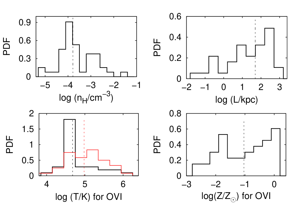
Figure 4.12: Distributions of density, thickness, temperature and metallicity of O vi absorbers obtained from Cloudy modeling. In the lower left panel, the temperature distribution derived from Cloudy models (black) is compared with that of upper temperature limit $T_{\rm max}$ (red) derived from the Doppler parameter. The dashed vertical lines in each panel mark the medium values in the samples.

The distributions of volume density $n_{\rm H}$, temperature $T$, metallicity $Z$ and absorption path length $L$ through a cloud, as derived through Cloudy, are plotted in Fig. 4.12. The density distribution (top left panel) is rather broad with a weak evidence for bimodality, with peaks at log $n_{\rm H}\approx-4.0$ and log $n_{\rm H}\approx-2.8$. This apparent bimodality might be caused by incompleteness effects that we are not able to treat statistically at this point. However, as one can see in Sect. 5.2.2, a small second peak at log $n_{\rm H}\approx-3.0$ is indeed expected from the OWLS which are more complete in a statistical sense. The median value of $\log\tilde{n}_{\rm H}=-3.8$ is typical for intergalactic absorbers.

Two temperature distributions of the O vi sample are plotted in Fig. 4.12, bottom left panel. The distribution derived from Cloudy modeling is juxtaposed with the one of the upper temperature limit $T_{\rm max}$ derived from the O vi Doppler parameter values assuming purely thermal line broadening (Eq. 2.23). The temperatures calculated from Cloudy are systematically lower than $T_{\rm max}$ – note the difference between the median values $\log\tilde{T}\approx 4.7$ and $\log\tilde{T}_{\rm max}\approx 5$. This result will be discussed in more details in Sect. 5.3.2, where it is compared to the results from the OWLS.

Note that the Cloudy modeling procedure mimics the observational approach: the metallicity is calculated from the total $N(\rm\mbox{O\,{\sc vi}\leavevmode\nobreak\ }\!\!)$/$N(\rm\mbox{O\,{\sc vi}\leavevmode\nobreak\ }\!\!)$ ratio. Later, in Sect. 5.2.3, we will introduce a second measure of the metallicity based on the OWLS and will discuss in more details the results from applying both metallicity definitions. The metallicity distribution of O vi systems, as derived from Cloudy, is characterized by median value (in log scale) of $-1.04$ dex (Fig. 4.12, bottom right panel). It appears bimodal, with peaks at $\log Z/Z_{\odot}\approx-1.8$ and $\log Z/Z_{\odot}\approx 0.0$. A similar bimodality in metallicity is found by Simcoe et al. (2006). However, their study includes all heavy elements, modeled with Cloudy. The authors suggest that the systems populating the zone around the higher-metallicity peak are probably produced by recent galaxy formation and feedback, while those around the lower-metallicity peak might trace older galactic debris. Interestingly enough, the bimodal tendency in the metallicity distribution of O vi absorbers is not confirmed by the OWLS (see Sect. 5.2.3).

Finally, we study the distribution of the absorption path length $L$ in the H i structure that contains O vi (Fig. 4.12, top right panel). It spans about five orders of magnitude: $0.01\leq L\lesssim 10^{3}$ kpc, with a median value $\tilde{L}\simeq 50$ kpc. Generally, O vi absorbers obviously arise in large-scale cosmological structures ($\log L\gtrsim 2$) as well as in local, small-scale structures. There is, however, an clear tendency that O vi absorbers with absorption path lengths $>10$ kpc are far more numerous than absorbers with smaller absorption path lengths.

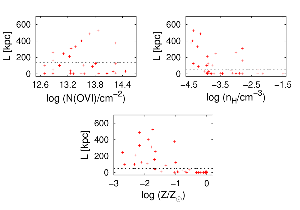
Figure 4.13: Correlation plots of some physical parameters obtained from the Cloudy models. The dashed line on the top left panel denotes a critical value for the absorption path length of $L=140$ kpc, while in the other cases it is plotted at $L=50$ kpc (see text).

We examine possible correlations between the parameters derived from Cloudy modeling in (Fig. 4.13). The O vi column density is put into relation with the absorber thickness $L$ on the top left panel. Clouds with smaller absorption path lengths (critical value: $L\approx 140$ kpc) seem to be homogeneously spread over the full column density range, while systems of high $L$ values exhibit a positive correlation between the thickness of the H i cloud and the O vi column density. The chosen critical value $L\approx 140$ demarcates two groups of systems: a population of local (small) structures and a population of the large scale structures. The most noticeable result from Fig. 4.13 is the absence of points in the upper right corners. If there were systems with high column densities/volume densities/metallicities and high absorption path lengths, they should be detectable. Systems with metallicities higher than 10 per cent of the solar solar value or with volume densities higher than $2\times 10^{-3}$cm^-3  display a maximum absorption path length of 50 kpc. A similar result is found by Simcoe et al. (2006), who suggest that the lack of data points in this parameter range might be explained by the fact that optically thick metal-enriched systems with higher gas densities are rare and have a small absorption-cross section.

4.4 Conclusions

In this chapter, we analyzed the statistical and physical properties of intervening O vi absorbers at high redshift based on a sample of 40 ($+$ 11) O vi systems observed with VLT/UVES. Our main conclusions could be summarized as follows:

• The calculated rate of incidence for the extended sample of 43 intervening O vi ​​ systems is $d\mathcal{N}/dz=5.2\pm 0.8$. The corresponding rate of incidence per absorption path length is $d\mathcal{N}/dX=1.6\pm 0.2$. Because of the imposed strong selection criteria, these values are slightly lower than previous estimates of the incidence rate of O vi absorbers at high redshift.

• About 30 percent of the basic (not extended) sample of 32 intervening O vi absorbers are single-component absorbers, while the remaining systems exhibit a more complex component structure. One third of the components in the single-component systems do not exhibit alignment with H i ​​, while this fraction increases with the number of O vi subcomponents.

• The median value of the Doppler parameter distribution from the UVES sample is 13.0 km s^-1 ​​, which corresponds to temperature $T_{\rm UVES}\sim 1.6\times 10^{5}$ K, assuming purely thermal broadening. The median column density value is log$N(\mbox{O\,{\sc vi}\leavevmode\nobreak\ }\!\!)=13.6$.

• The obtained power-law slope of CDDF at high redshift (using a completeness function) is $\beta\approx 1.10\pm 0.10$, when all points are included. The slope changes sensibly to $\beta\approx 1.51\pm 0.10$, imposing an apparent threshold of log$N(\rm\mbox{O\,{\sc vi}\leavevmode\nobreak\ }\!\!)\approx 13.3$ as a lower limit. Obviously the slope is very sensitive to the choice of a threshold.

• We calculate the cosmic density of O vi ​​ absorbers from the extended sample of 43 intervening systems in the redshift range $2.06\leq z\leq 2.91$. We derive a value of $\Omega_{{\footnotesize\rm\mbox{O\,{\sc vi}\leavevmode\nobreak\ }\!\!}}=3.3\times 10^{-7}$ for the full column-density range $11.5\leq\log N\leq 15.5$. The cosmological density of baryons, associated with the O vi absorbing phase is $\Omega^{{\footnotesize\rm\mbox{O\,{\sc vi}\leavevmode\nobreak\ }\!\!}}_{{\rm IGM}}/\Omega_{\rm b}=0.00856$ with $\Omega_{\rm b}=0.0418$. The fraction of baryons associated with O vi absorbers turns out to be less than 1 per cent of the total baryon density.

• We investigate the velocity widths $\delta v$ of the O vi absorbers in our UVES sample and their velocity offsets $\Delta v$ to the corresponding H i and C iv lines. We find that absorbers with small velocity offsets between O vi and H i ($\Delta v\leq 13$ km s^-1 ​​) represent kinematically simple, isolated gas structures. In contrast, O vi absorbers that have a significant velocity offset compared to H i appear to be embedded in a kinematically more complex host structure with a larger internal velocity dispersion, as expected, for instance, for gaseous material expelled from galactic winds and outflows.

• To investigate the physical conditions in kinematically aligned O vi ​​/H i absorbers, we model the ion column densities of selected absorbers from the UVES sample using the photoionization code Cloudy. The density distribution is rather broad with a weak evidence for a bimodality with peaks at log $n_{\rm H}\approx-4.0$ and log $n_{\rm H}\approx-2.8$. The temperatures derived under the assumption of photoionization are typically less than $10^{5}$ K. They are systematically lower than what is estimated from the O vi Doppler parameters, assuming pure thermal broadening. The absorption path length $L$ in the H i structures containing O vi spans about five orders of magnitude ($0.01\leq L\lesssim 10^{3}$ kpc), with a median value $\tilde{L}\simeq 50$ kpc. In general, O vi absorbers evidently arise in large-scale cosmological structures, as well as in local, small-scale structures.

In summary, the study of the UVES sample of O vi absorbers presented in this chapter demonstrates that their physical properties at high redshift are highly diverse, which indicates multiple origins of the O vi absorbing gas: in large-scale intergalactic gas structures as well as in small-scale interface regions between hot and cools gas clouds in multi-phase structures. The implications of these findings for the understanding of the origin of highly-ionized gas at high redshift will be discussed in Chapter 6. In the following Chapter 5, we describe the next steps in our systematic investigation of O vi systems: a study of a very large sample of O vi synthetic absorption spectra, generated from the cosmological OWLS that include star-forming galaxies and their intergalactic environment.

Chapter 5 A systematic study of O vi absorbers in the cosmological OWLS

This chapter is dedicated to another important aspect of our systematic investigation of intervening O vi ​​ absorbers at high redshift: namely, the use of cosmological simulations that include a proper treatment of the dynamics and physics of intergalactic and circumgalactic gas. We here study a large sample of O vi absorbers at high redshift in synthetic absorption spectra generated from the OverWhelmingly Large Simulations (OWLS) (Schaye et al., 2010). Details on the set-up of the synthetic absorption spectra are presented in Sect. 2.3.2. To understand the nature of high-redshift O vi absorbers in the context of the evolution of the distribution of hot, metal-enriched gas from high to low redshifts, we also compare the statistical properties of high-$z$ O vi absorbers with those at $z\approx 0$. To avoid repetitions, the low- and high-redshift runs of the OWLS are abbreviated hereafter as lOWLS ($z=0.25$)and hOWLS ($z=2.50$), respectively.

There are many advantages in using synthetic spectra from cosmological simulations to study absorption systems in the IGM. In particular, physical parameters like temperature, gas density and metal abundance can be obtained directly from the simulations. Here, we will focus on the analysis of the physical properties of a sample of O vi absorbers obtained from a fiducial run of the OWLS set dubbed REF_L100N512. The statistical results from the simulations will be compared to the properties of the O vi absorbers, as derived from the observations presented in the previous chapter.

5.1 Key observables

5.1.1 Column-density distribution

The column density distributions of observed (UVES) and simulated (OWLS) O vi ​​ components are shown in Fig. 5.1. The corresponding median values (in logarithmic scale) are 13.6 and 13.2, respectively. The higher median value in the observed sample can be explained by the lack of higher-column-density components in the OWLS (cf. Fig. 4.4). Another reason for this difference can be the higher S/N and the resulting lower O vi detection limit in the spectra from the simulations ($\log N$(O vi ​​) = 12.8).

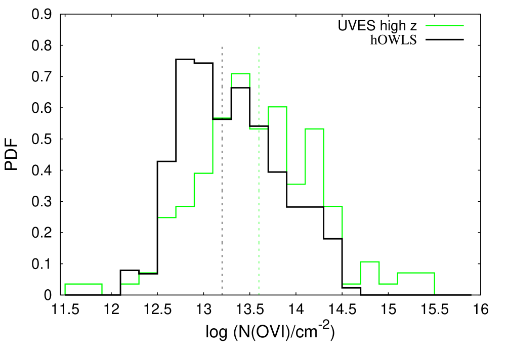
Figure 5.1: Column density distributions in the observational (blue) and simulated (black) high redshift sample. The positions of the medians are denoted with dashed lines.

In Fig. 5.2 we compare the CDDF derived from our UVES sample, as described in Sect. 4.2, with the one obtained from the simulations. The results of Bergeron & Herbert-Fort (2005) and Muzahid et al. (2012), who used a UVES data sample comparable to ours, are included for reference. The absorption path of the UVES data is $\Delta X=27.3$ (15 sight-lines), while that of the OWLS systems is $\Delta X=83.8$ (100 sightlines).

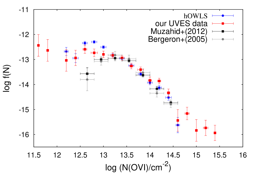
Figure 5.2: CDDFs derived from observations and simulations: from our UVES sample (red), from our sample of synthetic spectra (blue), from the UVES samples of Bergeron & Herbert-Fort (2005, grey) and Muzahid et al. (2012, black).

Our UVES sample appears to be complete down to $\log\leavevmode\nobreak\ N$(O vi ​​) $\approx 13.3$. Taking this threshold as a lower limit in the fitting procedure, we obtain a power-law slope $\beta_{\rm OVI}=1.51\pm 0.10$ (see Sect. 4.2). The detection limit for the synthetic spectra is $\log\,N$(O vi ​​) $=12.7$. Adopting this threshold, we obtain $\beta_{\rm OVI}=1.37\pm 0.07$. However, adopting a threshold of $\log\leavevmode\nobreak\ N$(O vi ​​) $\approx 13.3$ yields $\beta_{\rm OVI}=1.60\pm 0.11$ for the OWLS data, in agreement with the observations. As can be seen in the figure, all distributions agree within the uncertainties in the range $13.3\leq\log N$(O vi ​​)$\leq 14.6$. The power-law slopes of the CDDF derived by Bergeron & Herbert-Fort (2005) and Muzahid et al. (2012) are steeper, $\beta_{\rm OVI}=1.71\pm^{0.48}_{0.47}$ and $\beta_{\rm OVI}=2.4\pm 0.2$, respectively. The CDDF derived from our synthetic spectra is very similar to the one in Muzahid et al. (2012), if the bin of highest column density ($\log N$(O vi ​​) = 14.4) is excluded.

We perform power-law fits to the CDDF using our observed and simulated samples and those from Bergeron & Herbert-Fort (2005) and Muzahid et al. (2012) in the range $13.3\leq\log(N_{\rm OVI})\leq 14.6$ to assess the sensitivity of the slope to the adopted threshold. For this range, the slope of the data used by Muzahid et al. (2012) yields $\beta=1.56\pm 0.17$, close to the value from the OWLS: $\beta_{\rm OVI}=1.60\pm 0.11$. On the other hand, the slope, obtained from our UVES data is shallower: $\beta_{\rm OVI}=1.35\pm 0.16$, but still consistent with the other values. This is because of the relatively high number of O vi components with column densities $\log(N_{\rm OVI})\geq 14$ in our UVES data set compared to the O vi sample of (Muzahid et al., 2012) (see Fig. 5.2).

Also at higher column densities $\log(N_{\rm OVI})>14.6$, the hOWLS and UVES samples used by Bergeron & Herbert-Fort (2005) and Muzahid et al. (2012) exhibit a lack of components with respect to our observed UVES sample (Fig. 5.2, red squares). A similar trend apparently also exists in the lOWLS sample, as discussed in Sect. 5.1.2.

5.1.2 Distribution of Doppler parameters

Because of the expected turbulent motions in the gas, the value of the Doppler parameter derived from a Voigt-profile fit yields only an upper limit to the kinetic temperature of the gas (see also Sect. 2.1.2). Therefore, instead of setting constraints to the physical state of O vi systems from individual values of $b$ from the O vi absorption components, we consider their distribution.

The top panel of Fig. 5.3 displays the Doppler parameter distributions for the sample of observed and simulated O vi components. The median values are $\tilde{b}_{\rm UVES}=13\leavevmode\nobreak\ \rm km\leavevmode\nobreak\ s^{-1}$ and $\tilde{b}_{\rm OWLS}=15\leavevmode\nobreak\ \rm km\leavevmode\nobreak\ s^{-1}$ which correspond, assuming purely thermal broadening, to $T_{\rm UVES}\sim 1.6\times 10^{5}$ K and $T_{\rm OWLS}\sim 2.2\times 10^{5}$ K, respectively. The latter temperature is consistent with the estimate of Simcoe et al. (2002): $T\sim 2.1\times 10^{5}$ K, obtained from high-$z$ Keck I/HIRES observations. On the other hand, as mentioned in Sect. 4.2.2, $T_{\rm UVES}$ is close to the result of Muzahid et al. (2012): $T\sim 1.8\times 10^{5}$  K.

In the case of collisional ionization equilibrium (CIE), the temperature in O vi ​​ systems would peak around $T\approx 3\times 10^{5}$ K (Gnat & Sternberg, 2007; Sutherland & Dopita, 1993), which corresponds to $b\approx 17$ km s^-1 ​​. We note that 66 per cent of the components in OWLS sample and 68 per cent in the UVES sample have values of the Doppler parameter $<17$ km s^-1 ​​. This result suggests that photoionization is the main ionizing mechanism in these absorbers. At high metallicities, non-equilibrium collisional ionization might be an alternative mechanism.

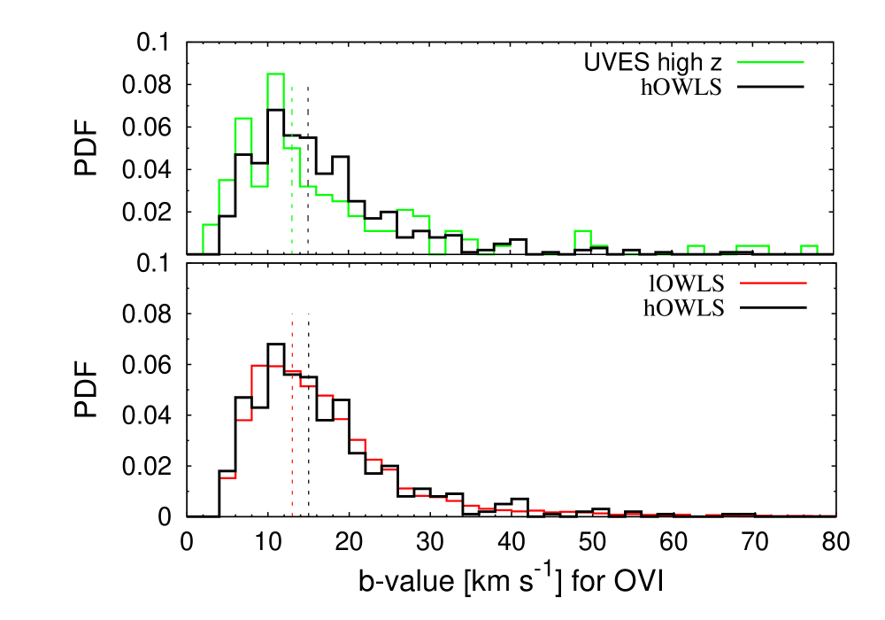
Figure 5.3: Comparison between the distributions of the Doppler parameter in the observed and simulated samples at high $z$ (top panel), and the Doppler parameter in lOWLS and hOWLS samples (bottom panel). The position of the median is indicated by dashed lines.

Gnat & Sternberg (2007) point out that in CIE the O vi fraction must be less than 0.01 at temperatures $T\geq 6\times 10^{5}$ K ($b$(O vi ​​)$\geq 25.5$ km s^-1 ​​). Therefore, one should not expect higher $b$(O vi ​​) values in case of purely thermal broadening unless the metallicity and/or $N(\rm H)$ are very high. We find 12 per cent of the components in the OWLS sample and 18 per cent of the components in the UVES sample with higher values of $b$ than 25.5 km s^-1 ​​.

5.1.3 Redshift-dependence of the line width

The Doppler parameter distributions from the lOWLS and hOWLS samples are compared in the bottom panel of Fig. 5.3. Evidently, both distributions are similar, with median values $\tilde{b}$ (O vi ​​)$=13$ km s^-1 for low $z$ and $\tilde{b}$ (O vi ​​)$=15$ km s^-1 for high redshift samples.

A similar comparison using observations has been done by Fox (2011) and Muzahid et al. (2012). Fox (2011) compares the low-$z$ sample of Tripp et al. (2008) with the high-$z$ sample of Bergeron & Herbert-Fort (2005). Muzahid et al. (2012) further compare the same sample of Tripp et al. (2008) with a two-times larger UVES high-$z$ sample. The median Doppler parameters of the O vi spectra found by these authors and other relevent parameters of their data are listed in Table 5.1. Tripp et al. (2008) obtain a median $\tilde{b}_{\rm STIS}\sim 26$ km s^-1 for the low $z$ sample. Fox (2011) and Muzahid et al. (2012) obtain $\tilde{b}_{\rm UVES}\sim 14$ km s^-1 at high $z$ and conclude that the O vi components are, on average, almost twice as broad at low-$z$ than at high-$z$. This finding does not agree with the result from our OWLS synthetic spectra. To investigate this, we have composed diagrams $N$(O vi ​​) vs. $b$ for the OWLS, UVES and STIS data (Fig. 5.4).

Table 5.1: Observational and technical parameters of reference works.

Study	Technical parameters			Observational parameters
	Spectrograph	Resolution	mean $S/N$	Redshift	Median $b$-value
		[km s-1 ​​]			[km s-1 ​​]
Tripp et al. (2008)	STIS/HST	7.0	13 at 1300 Å	$z<$ 0.5	26.0$\pm$14.0
Bergeron & Herbert-Fort (2005)	UVES/VLT	6.6	30-40 at 3300 Å	2.0 $\leq z\leq$ 2.6	14.0$\pm$7.0
Muzahid et al. (2012)	UVES/VLT	6.6	30-40 at 3300 Å	2.0 $\leq z\leq$ 2.6	13.8$\pm$14.0

Brief eye inspection already indicates the differences between the low-$z$ samples. There is a lack of components with high column densities and large $b$-values in lOWLS in comparison to the sample of Tripp et al. (2008) (left panels). Since the OWLS synthetic spectra mimic the spectral properties of STIS data, this difference cannot be attributed to the resolution or other instrumental characteristics. The reason for that mismatch between simulations and observations is still unclear. As pointed out by Tepper-García et al. (2011), one can rule out the explanation that the observed O vi systems arise in gas at higher temperatures (producing higher $b$-values), as this would result in a too low O vi ion fraction for either CIE or non-equilibrium ionizaion conditions.

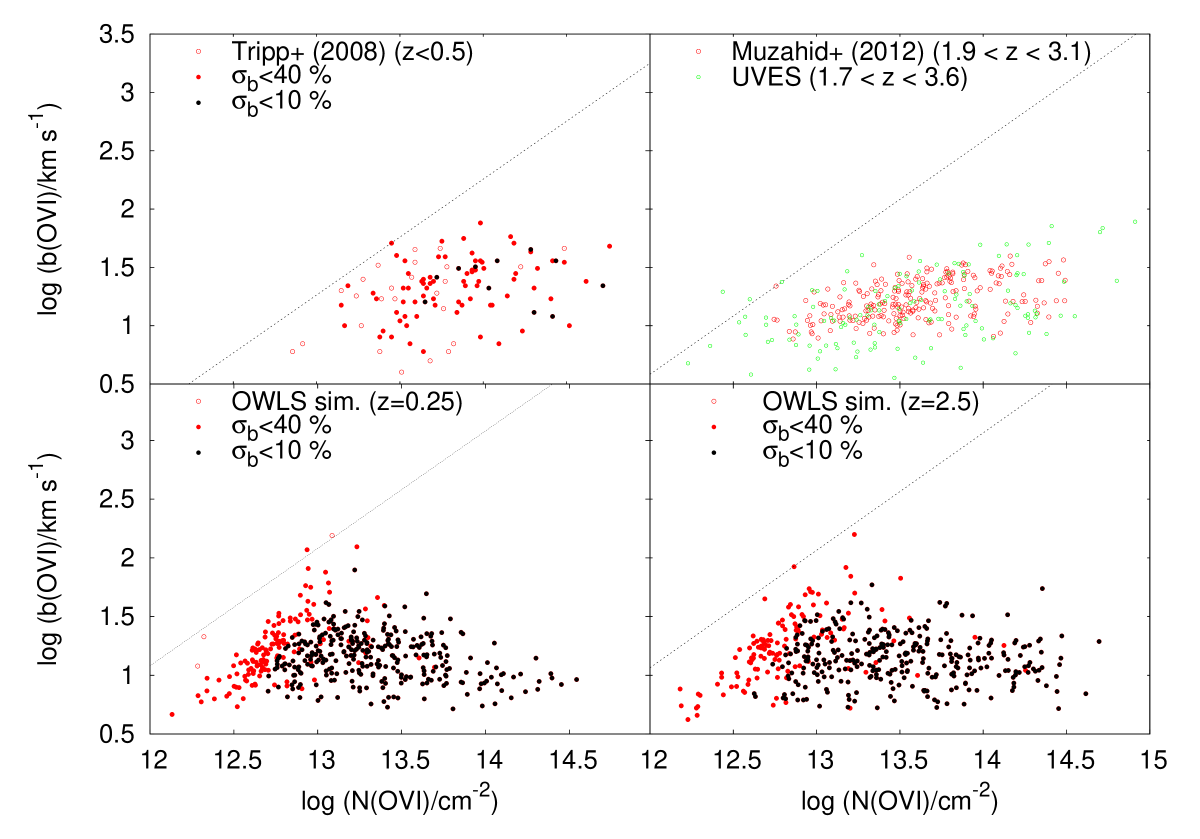
Figure 5.4: $N$ vs. $b$ from observed (bottom panel) and simulated (top panel) spectra at low $z$ (left panel) and high $z$ (right panel).

Similarly, a lack of systems with large $b$-values at low $z$ is found in the simulations of Oppenheimer & Davé (2009). Because the resolution achieved by current simulations does not allow to properly model turbulence at the smallest scales, these authors added a sub-resolution turbulent component to the thermal $b$-value. This brings the predicted distribution of equivalent widths into a better agreement with observations and suggests that turbulence plays a significant role in the line broadening at low $z$.

The physical picture at high $z$ is different. The similarity between the Doppler parameter distributions from synthetic and observed spectra suggests that non-thermal mechanisms at small scales do not significantly affect the O vi line widths. This will later allow us to combine the results from the simulations and observations to study the thermal evolution of O vi systems (see Sect. 5.3.2).

5.2 Physical conditions: high $z$ vs. low $z$

5.2.1 Temperature

The maximum kinetic temperature of clouds in photoionization equilibrium is $T\sim 40\leavevmode\nobreak\ 000$ K. Below this temperature, collisional ionization is not significant. The latter process dominates the ionization state of gas at $T\gtrsim 10^{5}$ K, regardless of the mean density. As mentioned in Sect. 5.1.2, the ionization fraction of O vi peaks at $T\approx 3\times 10^{5}$ K in CIE (Sutherland & Dopita, 1993; Gnat & Sternberg, 2007).

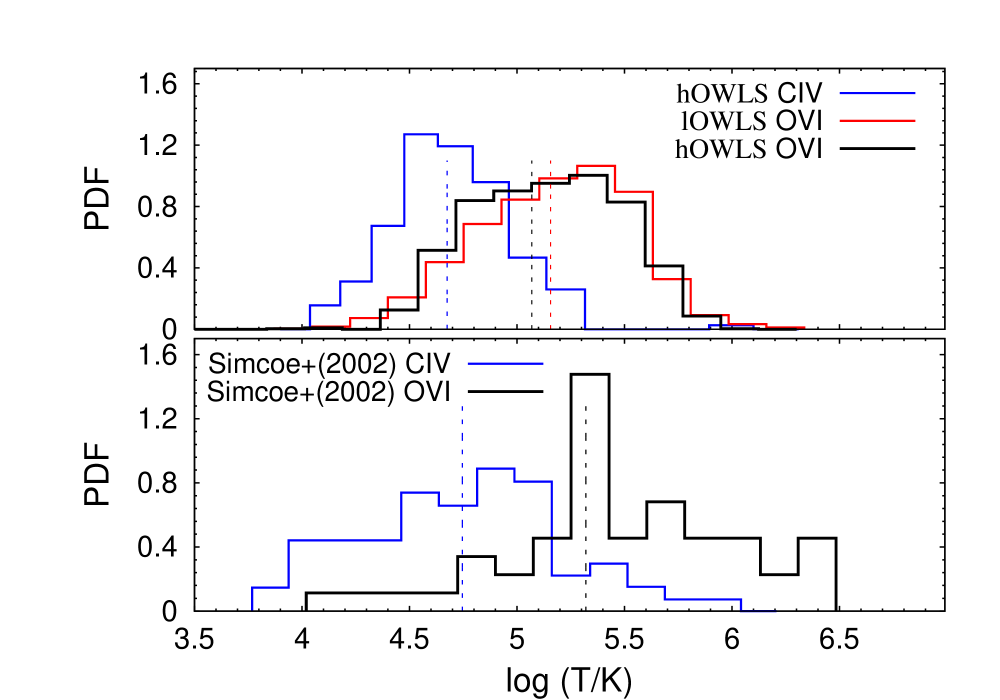
Figure 5.5: Temperature distributions of O vi absorbers from simulations (top panel) and observations (bottom panel). The distribution for C iv absorbers (blue) from the hOWLS sample (top panel) and from the sample of Simcoe et al. (2002, bottom panel) is plotted for comparison.

Simulations by Tepper-García et al. (2011) reveal a bimodal temperature distribution of the O vi bearing gas at low $z$, conditioned by photoionization at $T\approx 3\times 10^{4}$ K and by collisionally ionization at $T\approx 3\times 10^{5}$ K. However, the lower temperature regime is not significantly detected in O vi absorption. A possible explanation is a low oxygen abundance in the cool gas and, hence, a low O vi column density that prevents from tracing this gas phase in absorption.

Following Tepper-García et al. (2011), we consider optical-depth weighted physical quantities (e.g., temperature, density, metallicity) of the gas traced by the O vi absorption lines in the synthetic spectra. The optical-depth weighting relates an absorption-line profile to the absorbing gas in the simulation and allows us to compare the fitted parameters (Doppler parameter, column density) with the physical quantities given in the simulations.

The optical-depth weighted temperature distributions of O vi absorbers from the hOWLS 
(black) and lOWLS (red) samples are shown in Fig. 5.5. Additionally, both distributions are compared with the O vi temperature distribution by Simcoe et al. (2002) (black) in the redshift range 2.2 $<z<$ 2.8 . In the work of Simcoe et al. (2002) the temperature is calculated from formula (2.23), neglecting non-thermal broadening. Therefore it should be considered as an upper limit $T_{\rm max}$ of the gas temperature.

As seen in Fig. 5.5, the O vi temperature distributions derived from synthetic spectra at low and high $z$ are very similar, with almost identical median values: $1.4\times 10^{5}$ K and $1.2\times 10^{5}$ K, respectively. Sixty-five per cent of the lOWLS O vi seen in absorption traces mainly the hot gas phase at temperatures $T\geq 10^{5}$ K which is the low temperature regime of the WHIM (Tepper-García et al., 2011). The same trend is evident considering the hOWLS sample where 62 per cent of the components are hotter than $10^{5}$ K. Apparently, there is (on average) no temperature evolution of the O vi absorbers from high to low redshift. The O vi distribution from the hOWLS sample is in agreement with the result of Simcoe et al. (2002) who obtain from high $z$ observations a median value of $\widetilde{T}_{\rm max}$ = 2.1 $\times 10^{5}$ K. These authors also find that 62 per cent of all systems fall in the range $5.0\leq\log T_{\rm max}\leq 6.0$. A plausible mechanism that is able to produce O vi absorbers with such temperatures is collisional ionization in hot winds expelled from galactic environments.

We further compare the temperature distributions of O vi (black) and C iv (blue) absorbers (hOWLS sample, top panel; Simcoe et al. (2002), bottom panel). The difference is notable: about $0.6$ dex in log $T$ between the median hOWLS values. The same trend is found in the distributions by Simcoe et al. (2002). A comparison between the C iv temperature distributions from hOWLS and Simcoe et al. (2002) shows that they have almost identical median values: $4.6\times 10^{4}$ K and $4.7\times 10^{4}$ K, respectively. This implies that, considering both observed and synthetic spectra, the O vi lines are broader and arise in gas with physical conditions that are different from that of the C iv absorbing phase. The gas traced by the O vi absorption is hotter, while C iv is indicator of a cooler gas phase.

5.2.2 Density

As seen in Fig. 5.6 (top), the median values of the hydrogen densities in all O vi ​​ absorbers from the lOWLS and hOWLS samples differ by one order of magnitude: $8.7\times 10^{-6}$ cm^-3 vs. $8.7\times 10^{-5}$ cm^-3. This result suggests that O vi absorbers at low redshifts are produced in a more diffuse environment than those at high $z$.

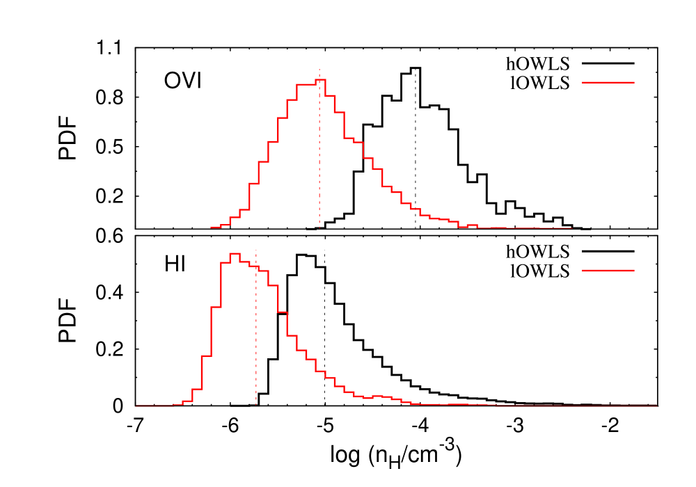
Figure 5.6: Hydrogen density distributions of all simulated O vi (top) and H i absorbers (bottom), at high (black) and low (red) redshift.

We also compare the hydrogen gas density distributions derived for all H i absorbers at low and high $z$ (bottom) with those of O vi absorbers. The pattern is the same – H i absorbers at low redshifts populate more diffuse regions in comparison to high $z$ systems. Most probably, this is an ionization effect: the photoionization rate $\Gamma_{-12}$ is an order of magnitude higher at $z=2$ than at $z=0$. Yet, in both cases, O vi absorption traces the densest regions of the H i absorbers.

A small second peak in the hOWLS O vi density distribution is seen at log $n_{\rm H}=-3.0$, which does not appear in the lOWLS O vi distribution. However, such a second peak is also seen in the O vi density distribution from the UVES observations (see Sect. 4.3).

5.2.3 Overall metallicity

The OWLS track the abundance of 11 individual elements (H, He, C, N, O, Ne, Mg, Si, Fe, Ca and S). They simultaneously keep record of the metallicity of each SPH particle (Wiersma et al., 2009b). The metallicity, as a parameter in the simulations, can be defined in two ways. The fraction of metals to the total gas mass in each SPH particle $Z_{\rm part}\equiv m_{Z}/m$ is called ‘particle metallicity’. The alternative definition of metallicity is $Z_{\rm sm}\equiv\rho_{Z}/\rho$, i.e. the ratio of the SPH smoothed metal mass density to the SPH smoothed gas mass density (see e.g. Okamoto et al., 2005; Tornatore et al., 2007). Hereafter, we will refer to this metallicity as ‘smoothed metallicity’, following Wiersma et al. (2009b).

Smoothed metallicity

In this section, we analyze the distribution of the optical-depth weighted smoothed metallicity $Z_{\rm sm}$(O vi ​​) of the gas as traced by O vi absorbers at high $z$ and compare it with that of the lOWLS sample. We stick to this definition of metallicity as it is more appropriate for the analysis of SPH simulations (Wiersma et al., 2009b). Moreover, as pointed out by Tepper-García et al. (2011), this choice takes into account the metallicity of each SPH particle that contributes to the O vi absorption. In other words, this quantity is a measure of the metallicity in small regions around the spatial resolution limit of the simulations while the observable $Z$ (O vi ​​), derived from the ratio of the total $N$(O vi ​​) to $N$(H i ​​), corresponds to metallicity of more extended host structures and can be substantially less than $Z_{\rm sm}$(O vi ​​). Hereafter, we call $Z$ (O vi ​​) the ‘mean metallicity’, like in Wiersma et al. (2009b) and Tepper-García et al. (2011).

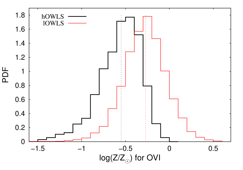
Figure 5.7: Metallicity distributions of simulated O vi absorbers from the hOWLS (black) and lOWLS (red) data samples.

The metallicity distributions of O vi absorbers from the hOWLS and lOWLS samples are plotted in Fig. 5.7. Apparently, O vi absorbers at high $z$ trace metal-enriched material with $\log(Z_{\rm sm}$(O vi ​​)/$Z_{\odot})>-1.5$ and a median value $\widetilde{Z}_{\rm sm}$(O vi ​​)$\approx 0.3\leavevmode\nobreak\ Z_{\odot}$. The median for the lOWLS sample is closer to the solar value $\widetilde{Z}_{\rm sm}$(O vi ​​) $\approx 0.6\leavevmode\nobreak\ Z_{\odot}$. The increase of $Z$ from high to low redshifts is consistent with most models of cosmic chemical evolution that predict a rise of the global mean interstellar metallicity in galaxies with time, reaching quasi-solar values at $z=0$ (see e.g. Pei & Fall, 1995; Malaney & Chaboyer, 1996; Pei et al., 1999; Somerville et al., 2001).

Mean metallicity

Structures with measurable O vi absorption are traced by well-aligned O vi ​​/H i ​​ absorber pairs within some small velocity range $\Delta v$. Following Tepper-García et al. (2011), we adopt $\Delta v\pm 10\leavevmode\nobreak\$km s^-1 and select by this criterion a subsample of aligned absorbers to investigate their metallicity distribution. Proximity in velocity space between H i and O vi lines most probably indicates that these species arise in the same gas phase or, at least, in the same overall gas structure. The mean metallicity $Z$(O vi ​​) of the absorber is calculated according to the formula:

$$Z(\small{\rm OVI)}=\Big{(}\frac{N_{\rm\small{\rm OVI}}}{N_{\rm\small{\rm HI}}}\Big{)}\Big{(}\frac{f_{\rm\small{\rm HI}}}{f_{\rm\small{\rm OVI}}}\Big{)}\Big{(}\frac{m_{\rm O}}{m_{\rm H}}\Big{)}X_{\rm H}$$ (5.1)

where $m_{\rm H}$ and $m_{\rm 0}$ are the masses of hydrogen and oxygen atoms, $f_{\rm\small{\rm HI}}$ and $f_{\rm\small{\rm OVI}}$ are the optical-depth weighted ionization fractions, $N_{\rm\small{\rm HI}}$ and $N_{\rm\small{\rm OVI}}$ are the column densities of H i and O vi , and $X_{\rm H}$ is the hydrogen fraction.

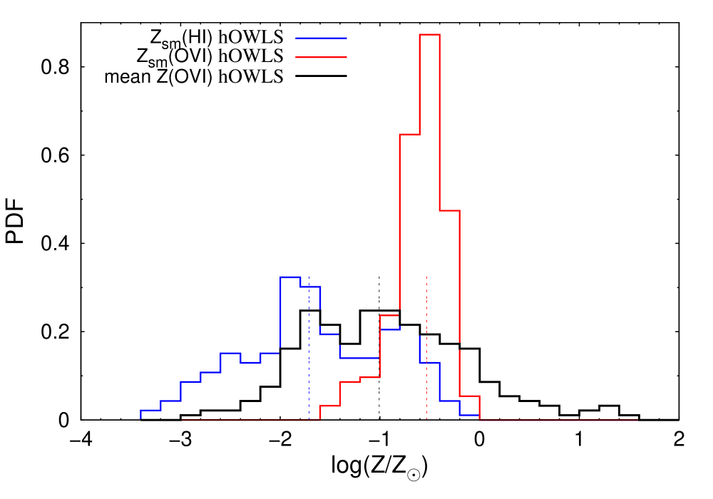
Figure 5.8: Metallicity distributions of simulated well-aligned H i (blue) -O vi (red) absorber pairs at high $z$. The metallicity distribution based on an estimate of $Z$ from the O vi ​​/H i column density ratio is plotted for comparison (black).

The distributions of the resulting metallicities for all well-aligned pairs $Z_{\rm sm}$(H i ​​) and $Z_{\rm sm}$(O vi ​​) are shown in Fig. 5.8. It is evident that the distribution of $Z$(O vi ​​) has a larger dispersion than that of $Z_{\rm sm}$(O vi ​​). The median values are 10 per cent of the solar metallicity and 30 per cent of the solar metallicity, respectively. The peak of the $Z$(O vi ​​) distribution is at higher metallicities in comparison to the distribution of $Z_{\rm sm}$(H i ​​), but similar in width. These results are similar to those of Tepper-García et al. (2011) from low-redshift OWLS: the mean metallicity of the absorbing structures can be very different from the smoothed metallicities due to the possible concentration of the metals in small, tiny subregions as represented by the quantity $Z_{\rm sm}$(O vi ​​). As suggested by these authors, a possible interpretation might be a highly inhomogeneous distribution of $Z$, where the O vi absorbers arise in high- metallicity regions embedded in a lower-mean-metallicity gas phase.

5.2.4 Oxygen abundance

In addition to the overall metallicity we compute the oxygen abundance, [O/H], of the well-aligned H i and O vi ​​ synthetic absorption components, derived from their column-density ratios and ion fractions. In order to compare our result with the oxygen abundance from observations, obtained by Bergeron & Herbert-Fort (2005) we assume the same solar relative abundanses used by this authors (Anders & Grevesse, 1989). Bergeron & Herbert-Fort (2005) analyze a sample of O vi absorbers in the redshift range $2.0\leq z\leq 2.6$, using spectral data of 10 quasars from UVES observations. Their estimate of the oxygen abundance is calculated under the assumption of photoionization as the only ionization mechanism, while the simulations we use include both photoionization and collisional ionization. The two distributions are shown in Fig. 5.9. The median value for OWLS synthetic spectra is $-1.35$ dex, which is higher than the median value of Bergeron & Herbert-Fort (2005) ($-1.75$ dex). The ranges of both abundance distributions are around $-3.0\leq[\rm O/H]\leq 1.0$.

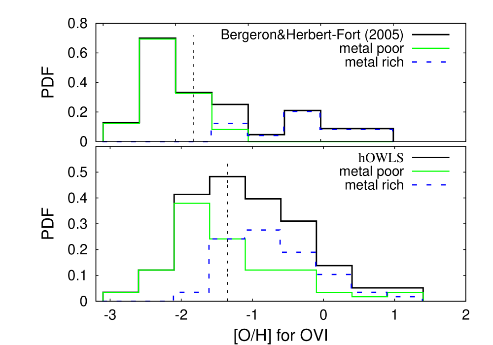
Figure 5.9: Distribution of oxygen abundance in the sample of simulated well-aligned H i ​​/O vi ​​ absorber pairs at high $z$ (bottom panel). The observational result of Bergeron & Herbert-Fort (2005) for redshift range $2.0\leq z\leq 2.6$ is plotted for comparison (top panel). The distribution is divided in the two populations – ’metal-rich’ and ’metal-poor’ absorbers. The position of the median is denoted with dashed lines.

As a next step, we continue our investigation of metal-rich and metal-poor absorbers, proposed by Bergeron & Herbert-Fort (2005) (see Sect. 4.2.1). The result of this authors is plotted in Fig. 5.9, top panel. The [O/H] distributions of the two populations overlap slightly. From this, the authors concluded that O vi absorbers indeed represent two distinct populations. To reevaluate this result, we use their observational criteria and divide our absorbers in two sub-samples: metal-rich and metal-poor (see Sect. 4.2.1), based on the O vi and H i column-density ratios. Our result is plotted in Fig. 5.9, bottom panel. In contrast to the result of Bergeron & Herbert-Fort (2005), we find a significant overlap between the abundance distributions of metal-rich and metal-poor populations. We also derive their $b$-value distributions (not shown) and find again an overlap, including the high velocity tails. Our results from the simulations suggest that there is no compelling evidence for the existence of such two distinct populations of O vi absorbers.

5.3 Discussion on physical parameters and observables of the OVI absorbers

In the first part of this section we analyze possible correlations between global physical parameters of the absorbers (weighted by optical depth; e.g., gas temperature, gas density and smoothed metallicity) and key observables such as column density and Doppler parameter. Such correlations can provide clues to our understanding of the nature and the origin of the O vi absorbers at high redshift.

In the second part of this section a subsample of well-aligned (in velocity space)  O vi ​​/H i and O vi ​​/C iv pairs is considered. This part of the study will be directly connected to the results from our UVES observations, as these provide key observables like column density and Doppler parameter, whereas the physical properties of the absorbers can be constrained only based on certain assumptions (see also Chapter 3). One of these assumptions is, that the different ions coexist in the same gas-phase. A common approach for observers therefore is, to look for an alignment in velocity space, which usually is interpreted as evidence that the observed species reside in the same physical region. However, this assumption introduces systematic uncertainties in modeling the physical state of the gas: an alignment in velocity space does not necessarily imply a true spatial alignment and a common gas-phase, but could be just the result of overlapping radial velocities and similar bulk motions. Therefore, we take the advantage of using cosmological simulations to extract information about true physical conditions in the absorbing gas. Then, we are able to systematically investigate, whether the usual assumption of the coexistence of O vi , H i , and C iv in a single gas phase for well-aligned absorbers in observational data is really justified.

5.3.1 All absorbers

Doppler parameter vs. column density

One possible correlation to look for is the one between the Doppler parameter and the column density in the absorber. Such a correlation might be present because of a number of different effects: undetected velocity structure in absorbers of higher column density, collisional ionization that links column densities in highly ionized systems and temperature, or selection effects (since broad, weak lines are hardly detectable in the noise).

Different research groups had searched for such a correlation at low redshifts. Heckman et al. (2002) found a correlation between $b$ and $N$ in their sample of observed O vi systems in a variety of environments: Milky Way disk and halo, High-Velocity Clouds, the Magellanic Clouds, and the IGM. These authors suggested that above $\log b\approx 1.6$ the column density increases linearly with line width, while the relation steepens for lower linewidths. However, Danforth et al. (2006) did not find such correlation from the analysis of their low $z$ data. Tripp et al. (2008) found a weak correlation in their observed O vi sample, but noted that the significance is not high enough to support the model of Heckman et al. (2002). Tepper-García et al. (2011) studied this issue further, considering a low-redshift O vi sample from OWLS synthetic spectra. They do not find a significant correlation between the O vi linewidths and column densities (see their Fig. 2, bottom right panel).

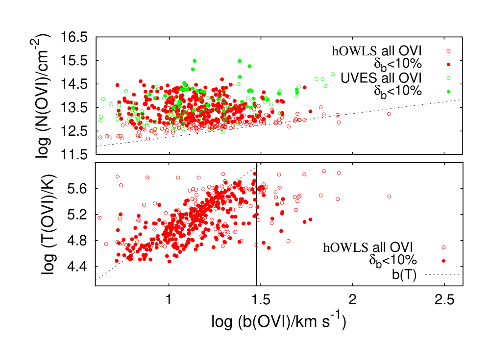
Figure 5.10: Correlation plots of the Doppler parameter from observational and synthetic spectra. A diagram $b$ vs. $N$ for the full OWLS sample of O vi absorbers (top panel) with its detection limit (dashed line) and a diagram $b$ vs. $T$ for the full samples of O vi absorbers (bottom panel) with UVES (green) and OWLS (red) data are shown. The subsamples with $\delta b\leq 10$ per cent are shown with filled symbols. The upper temperature limit (assuming purely thermal broadening) is drawn with a dashed line. The solid vertical line points to the the $b$-value above which the non-thermal broadening becomes the dominating factor.

A possible correlation between the Doppler parameter and column density at high redshifts has not been investigated intensively so far. Carswell et al. (2002) do not find a correlation in their UVES O vi data for two sightlines (see their Fig. 15). Muzahid et al. (2012) find a statistically insignificant correlation, considering an extended UVES O vi sample (18 sightlines).

Motivated by these studies, we have searched for a correlation between the Doppler parameter and column density in our simulated O vi absorber sample. The results are shown in Fig. 5.10 (top panel). No evidence for a correlation between the two quantities is found.

Doppler parameter vs. temperature

The temperature is another important physical quantity that governs the ionizaion state of the gas. A standard approach to estimate gas temperature, used by us in Sect. 4.3 and Appendix B for the analysis of the high-redshift UVES data, is, to consider the linewidths of observed absorber pairs O vi ​​/H i that are well aligned in velocity space. It should be pointed out that velocity alignment does not necessarily indicates that the considered absorbers arise in the same gas phase. We revisit the applicability of this method in Sect. 5.3.2. Due to its ambiguity, different authors obtain different temperature estimates in low-redshift absorbers (Thom & Chen, 2008; Tripp et al., 2008; Danforth & Shull, 2008). Therefore, it is interesting to look for (and to study) a possible correlation between O vi linewidth and gas temperature in our data. The correlation plot is shown in Fig. 5.10, bottom panel. Points that lie above the upper temperature limit (under assumption of purely thermal broadening) are caused by resolution effects and the fitting procedure (Tepper-García et al., 2011). There is a clear tendency of increase of gas temperature with the Doppler parameter. For $b>30$ km s^-1 (solid line in Fig. 5.10) non-thermal broadening becomes the dominating factor, leading to a larger $b$ for a given temperature than expected from purely thermal broadening. A qualitative conclusion is evident: generally, linewidths are representative for the real temperature, at least in a statistical sense. For temperature estimates of individual absorbers, however, one needs additional information, e.g. from supplementary data of other related ions.

Temperature vs. density

The distribution of O vi absorbers at $z=2.5$ on the gas density-temperature plane is shown in Fig. 5.11. The absorbers populate a region with corresponding densities of $10^{-5}\leq n_{\rm H}\leq 4\times 10^{-3}$cm^-3(overdensities $1.23<\Delta<4.9\times 10^{2}$) and temperatures $4\times 10^{4}\leq\rm T\leq 1\times 10^{6}$ K. Such overdensities reach four to five times higher values than the typical value for the WHIM ($\Delta\approx 0.1-100$). More than 60 per cent of all O vi absorbers are found in the low temperature regime of the WHIM, i.e. $10^{5}<\rm T<10^{6}$ K. The high temperatures indicate shock-heated material. Twenty-five per cent of the sample (red area) exhibit a tendency of decreasing of temperature with increasing gas density, although the correction is weak.

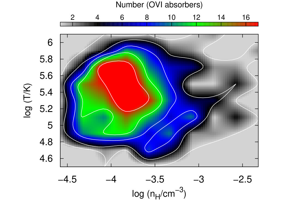
Figure 5.11: Distribution of all absorbers from the OWLS sample on the plane $T$ vs. $n_{\rm H}$ (see text). The colour scale indicates the distribution amplitude. The red/green/blue/black/gray areas and the white contours enclose 25/50/75/90/99 per cent of the total number of absorbers, respectively.

We study also the possible anti-correlation between temperatures and column densities of O vi absorbers, since it links an observed quantity with a physical parameter that is known directly from the simulations. Fig. 5.12 shows the distribution of all O vi absorbers from the hOWLS sample on the temperature-column density plane.

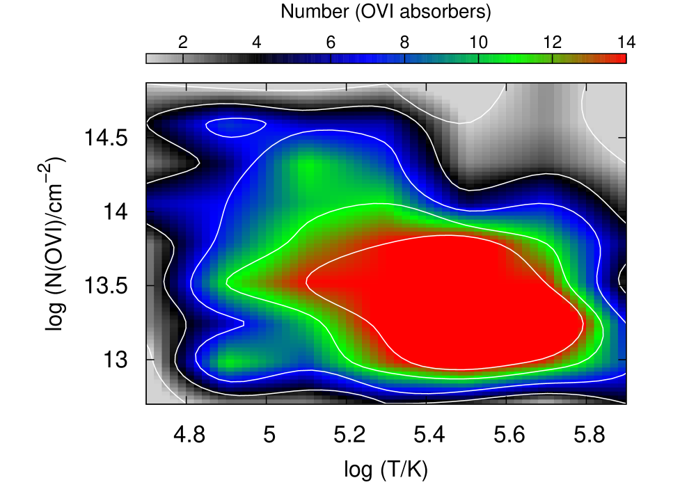
Figure 5.12: Distribution of all absorbers from the hOWLS sample on the plane $N_{\rm OVI}$ vs. $T$. The colour scales and contours are similar to the one used in the previous figure.

The bulk of O vi absorbers is found in the column-density range $10^{13}\leq N$(O vi ​​) $\leq 10^{14}$cm^-2. The temperatures $10^{5}\leq\rm T\leq 10^{6}$ K hint at shock-heated material. A high fraction (>50 per cent) of all O vi absorbers exhibit temperatures $T>10^{5}$ K and column densities $N$(O vi ​​) < $10^{14}$cm^-2. Systems with lower column densities tend to have higher temperatures, but no definitive conclusion about individual absorbers can be reached.

Column density vs. metallicity

We inspect a possible correlation between the metallicity $Z_{\rm sm}$(O vi ​​) and the column density of O vi , considering the full OWLS sample of O vi absorbers. Their distribution on the column density-metallicity plane is shown in Fig. 5.13.

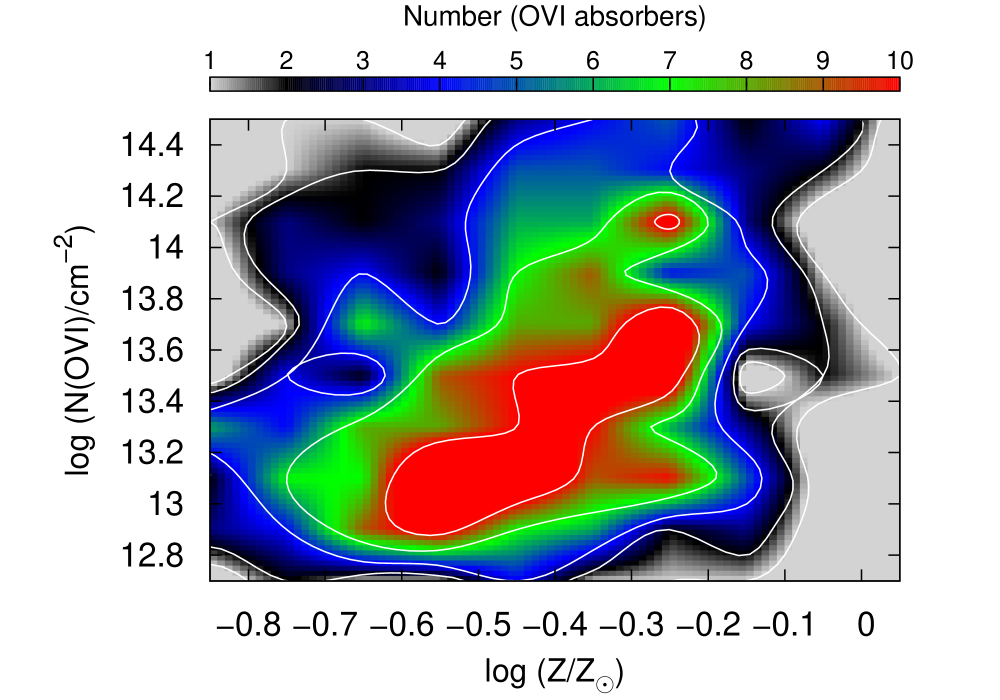
Figure 5.13: Distribution of all absorbers from the OWLS sample on the plane $N_{\rm OVI}$ vs. $Z$. The colour scales and contours are similar to the one used in the previous figure.

Such a correlation is indeed present for a subsample of absorbers that includes 25 per cent of the systems (red area). With a rise of column density in the range $12.8\leq\rm log(N$(O vi ​​)/$\rm cm^{-2})\leq 14.2$ the metallicity increases as well from $\sim-0.7$ dex to about $-0.2$ dex. It is clear from the figure that O vi synthetic absorbers trace enriched material with metallicities $\rm log(Z_{\rm sm}$(O vi ​​)/$Z_{\odot})\geq-1.5$, as already discussed in Sect. 5.2.3.

Temperature vs. metallicity

Finally, we plot the distribution of O vi absorbers at $z=2.5$ on the temperature-metallicity plane (Fig. 5.14). The majority of the absorbers lie within the temperature range $4\times 10^{4}\leq\rm T\leq 10^{6}$ K and in the metallicity range $-1.0\leq\rm\log(Z_{\rm sm}$(O vi ​​) $\leq 0.0$. About half of the sample (red and green areas) is constrained within a rather narrow metallicity range $-0.6\leq\rm\log(Z_{\rm sm}$(O vi ​​) $\leq-0.1$ and exhibit a tendency toward slight decrease of $\rm Z_{\rm sm}$(O vi ​​) with increasing temperature.

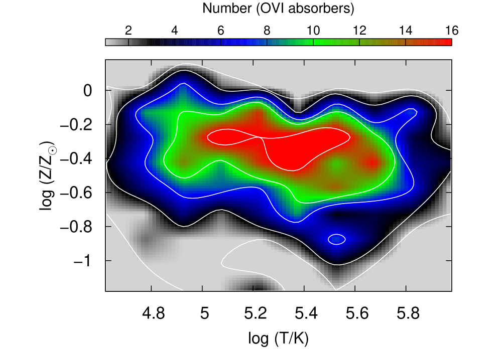
Figure 5.14: Distribution of all absorbers from the OWLS sample on the plane $Z$ vs. $T$. The colour scales and contours are similar to the one used in the previous figure.

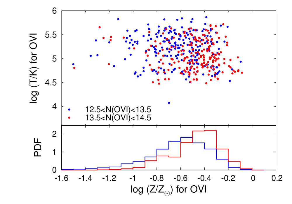
Figure 5.15: Metallicity vs. temperature for all O vi absorbers from the hOWLS sample. Top panel: two subsamples with $12.5\leq\rm log(N(\mbox{O\,{\sc vi}\leavevmode\nobreak\ }\!\!/{\rm cm}^{-2})\leq 13.5$ (blue) and $13.5\leq\rm log(N(\mbox{O\,{\sc vi}\leavevmode\nobreak\ }\!\!)/{\rm cm}^{-2})\leq 14.5$ on the $Z$ vs. $T$ diagram. Bottom panel: the metallicity PDFs of the subsamples.

In an attempt to distinguish a possible effect of column density on metallicity and/or temperature of the absorbers, we divided the hOWLS sample in two subsamples, according the column densities, and plotted them on the $T$ vs. $Z$ plane (Fig. 5.15, top panel). Evidently, systems with higher column densities tend to have higher metallicities as illustrated as well by the PDF distributions of metallicity (bottom panel). The Kolmogorov-Smirnov test yields a 0.42 probability that the two distributions have the same origin.

5.3.2 Aligned absorbers

Thermal and non-thermal components of the Doppler parameter in the aligned O vi absorbers

To explore the contribution of the non-thermal processes in the line broadening at high and low redshift (see Sec. 5.1.2), we consider a subsample of O vi absorbers that exhibit velocity alignment between O vi and H i ($\leq 10$ km $\rm s^{-1}$).

The Doppler parameter $b$, as introduced in Sect. 2.1.2, provides only an upper limit of the temperature on the absorbing gas. If the line broadening is influenced also by non-thermal mechanisms such as turbulence or peculiar velocities, the true temperature $T$ in an absorber is lower. The thermal and the non-thermal component of the Doppler parameter as defined by Eqs 2.23 and 2.25 are:

$$b^{2}=b^{2}_{\rm th}+b^{2}_{\rm nt}=(0.129)^{2}\leavevmode\nobreak\ \frac{T}{A}+b^{2}_{\rm nt}.$$ (5.2)

For ions located in the same physical region, the nonthermal component is assumed to be identical, whereas the thermal component scales inversely with the mass of the ion.

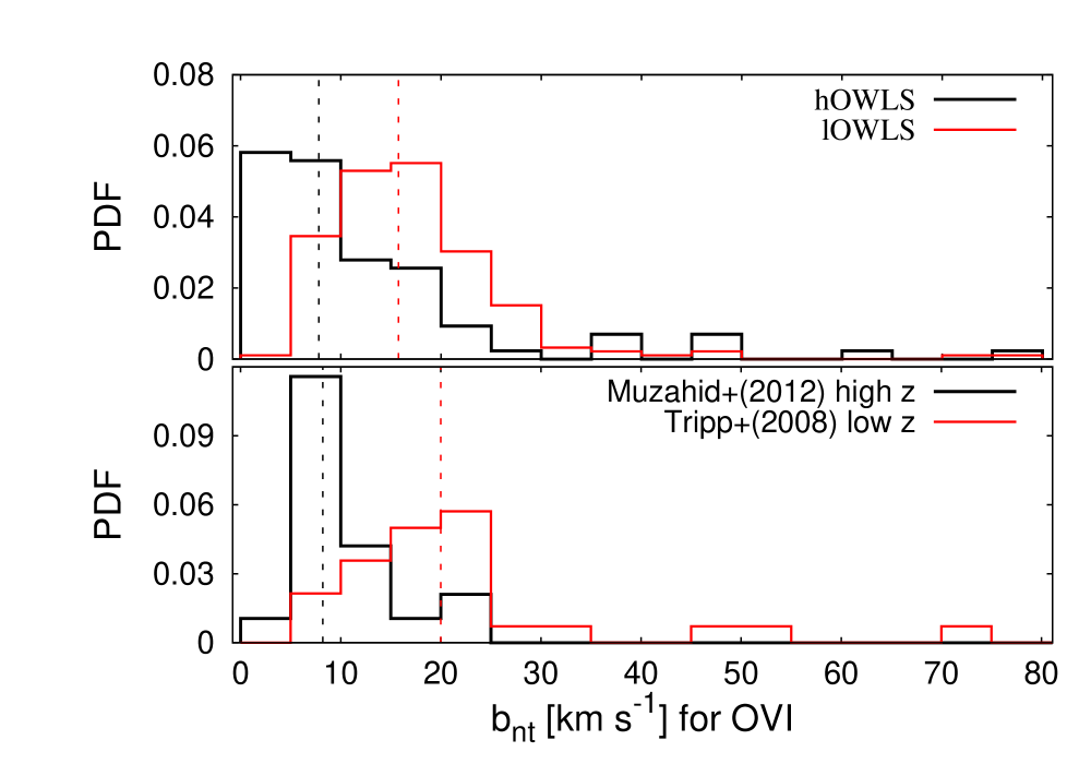
Figure 5.16: Distributions of $b_{\rm nt}$ for the well-aligned system components ($\Delta v=10\leavevmode\nobreak\ \rm km\leavevmode\nobreak\ s^{-1}$) in 5 $\rm km\leavevmode\nobreak\ s^{-1}$ bins detected in simulated (top) and observed (bottom) spectra at low and high $z$.

Since the lOWLS and hOWLS data provide information about the temperature for each ion, one can obtain $b_{\rm nt}$ (Eq. 5.2) for $b_{\rm th}$ of the aligned components (Eq. 2.23). In Fig. 5.16 the derived distributions of $b_{\rm nt}$ for low and high $z$ are compared with results from observational studies of Tripp et al. (2008) and Muzahid et al. (2012). In both observational studies $b_{\rm nt}$ was calculated from the total Doppler parameter using the following approach. First, O vi and H i components that are well aligned in velocity space were selected. The underlying assumption is, that these elements arise in the same gas phase. Second, two versions of Eq. 5.2 have been employed for H i and O vi to solve for $T$ and $b_{nt}$.

As seen in Fig. 5.16, the median $b_{\rm nt}$ for the low $z$ observations (Tripp et al., 2008) is $\sim$20 $\rm km\leavevmode\nobreak\ s^{-1}$, which is similar to the one obtained from the lOWLS synthetic spectra (15.75 $\rm km\leavevmode\nobreak\ s^{-1}$). For high $z$, the medians from hOWLS and from observations of Muzahid et al. (2012) are also almost identical: 7.8 $\rm km\leavevmode\nobreak\ s^{-1}$ and 8.2 $\rm km\leavevmode\nobreak\ s^{-1}$, respectively. Despite the similarity between the $b_{nt}$ distributions in the synthetic and the observed spectra at high and low $z$, we note that interpretation of this result is not straight-forward. The non-thermal Doppler parameter components are estimated by use of two very different approaches, as outlined above. Nevertheless, the result suggests that the $b_{\rm nt}$ distributions at high and at low $z$ are essentially different and it seems that this supports our previous scenario, namely that the nonthermal processes play a more important role at low redshifts (see Sect. 5.1.3). Therefore, the previous assumption, that the mean O vi line widths at high $z$ provide a rough estimate of the temperature of the absorbing gas, is justified.

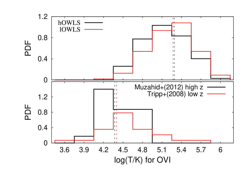
Figure 5.17: Temperature distribution of the H i ​​/O vi absorber pairs ($\Delta v=10\leavevmode\nobreak\ \rm km\leavevmode\nobreak\ s^{-1}$) at low (red) and high (black) $z$ from observed (bottom panel) and simulated (top panel) spectra.

The corresponding temperature distributions for the well aligned O vi absorbers at low and high $z$ are plotted in Fig. 5.17. The temperature from the observed spectra is calculated by consideration of $b(\mbox{H\,{\sc i}\leavevmode\nobreak\ }\!\!)-b(\mbox{O\,{\sc vi}\leavevmode\nobreak\ }\!\!)$ pairs, as described briefly in the beginning of the section. The conclusion drawn by Muzahid et al. (2012) is, that the temperature distribution for the low $z$ observational sample does not differ significantly from the one derived in their high $z$ observational study – the probability that the difference is statistical artifact is estimated to be $\approx$ 38 per cent. These authors point out that 42 per cent of their sample exhibits temperatures 4.6 $\leq$ log $T$ $\leq$ 5.0, which are higher than those expected from photoionization equilibrium. The suggested explanation is, that higher temperatures can be reached in a rapidly cooling over-ionized gas phase that was shock-heated through mechanical processes such as galactic winds.

However, the median of the temperature distribution in both observational samples is $\sim 3\times 10^{4}$ K, while the median value of the temperature distribution in both simulational samples is $\sim 1.9\times 10^{5}$ K, i.e., about one order of magnitude higher than found from observations.

Temperature distribution of the aligned O vi absorbers

The difference between the temperature distributions found from observational and simulated spectra of well-aligned O vi absorbers at high $z$ is puzzling. Looking for an explanation, we recall our previous conclusion that the non-thermal processes do not significantly affect the line broadening at high $z$ (see Sect. 5.1.2). Note that we calculated the upper limit of temperature, $T_{\rm max}$, from the $b$ values in the UVES subsample of well aligned O vi absorbers (see Sect. 4.3), assuming purely thermal broadening (Eq. 2.23). In Fig. 5.18 (bottom panel) the distribution of $T_{\rm max}$ is plotted together with the distribution of temperatures obtained from the Cloudy modeling for the same subsample of O vi absorbers. We added, for comparison, the O vi temperature distribution derived by Muzahid et al. (2012) (violet). The temperature distributions of O vi absorbers derived from the OWLS synthetic spectra, together with those of C iv and H i systems that are well aligned with them, are shown in the middle and top panels of this figure, respectively.

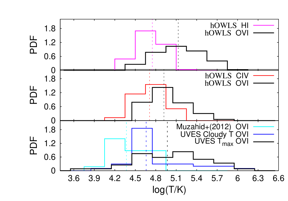
Figure 5.18: Temperature distributions of the well-aligned O vi components ($\Delta v=10\leavevmode\nobreak\ \rm km\leavevmode\nobreak\ s^{-1}$) at high $z$ as derived from different data. Bottom panel: our UVES sample, assuming purely thermal broadening (black) and from the Cloudy modeling (blue), and the UVES sample of Muzahid et al. (2012, violet); Middle panel: OWLS synthetic O vi components (black) and OWLS synthetic C iv components aligned with them (red); Top panel: OWLS synthetic O vi components (black) and OWLS synthetic H i components aligned with them (green). The dashed lines indicate the corresponding median values.

As can be seen in this figure, the samples of C iv and H i synthetic components aligned with O vi exhibit similar temperature distributions with median values $\log\,T=4.71$ and $\log\,T=4.75$, respectively. In contrast, the O vi distributions differ from them, depending on whether O vi is aligned with C iv or with H i ​​. The distribution of oxygen absorbers, aligned with H i (Fig. 5.18, top panel) is shifted to higher temperatures with a median value $\log\,T=5.13$. This result hints at different physical conditions and different gas phases, regardless of the velocity alignment. Better agreement, marked by a significantly closer median value $\log\,T=4.92$ is found with the distribution of the aligned C iv components (middle panel). In this case, it seems much more likely that the components of both species trace the same physical conditions.

A similar pattern in the temperature distribution of O vi absorbers is seen, when the UVES subsample of well aligned H i ​​/O vi pairs (Fig. 5.18, bottom panel) is considered. In case the temperature is calculated from the observed O vi $b$-values, assuming purely thermal line broadening, the median value of the O vi distribution is $\log\,T\approx 5$ (black line). However, when one assumes that O vi originates in the same gas phase as H i (and C iv ​​, in some cases) and models the physical conditions with Cloudy, the predicted median value $\log\,T\approx 4.66$ for the same UVES O vi subsample (blue line) is close to those of the C iv and H i distributions from the synthetic spectra. The distribution itself becomes more similar – although with a more extended high-temperature tail, – to the one derived by Muzahid et al. (2012, violet line), whose temperature calculations were based also on the assumption of a single gas phase for the observed O vi and H i systems. Apparently, the temperature distribution of the O vi components depends strongly on the chosen model, namely, whether the O vi lines arise in gas phase that is similar or different from that of C iv and H i ​​. Therefore, it is important to explore further, how reliable the assumption is that well-aligned components O vi ​​, C iv and H i actually arise in a single gas phase.

Clearly, if two or more ions are in a state of local ionization equilibrium and arise in the same gas phase, their corresponding absorbers trace the same physical region with one and the same gas temperature. Therefore, a comparison between the temperatures derived for O vi ​​, C iv and H i in well-aligned absorption components in the OWLS synthetic spectra would provide valuable information on this scenario. Such temperature/temperature diagrams for well-aligned O vi ​​/C iv and O vi ​​/H i components are plotted in Fig. 5.19, bottom panel. In the top panels the corresponding distributions of the velocity offsets are shown.

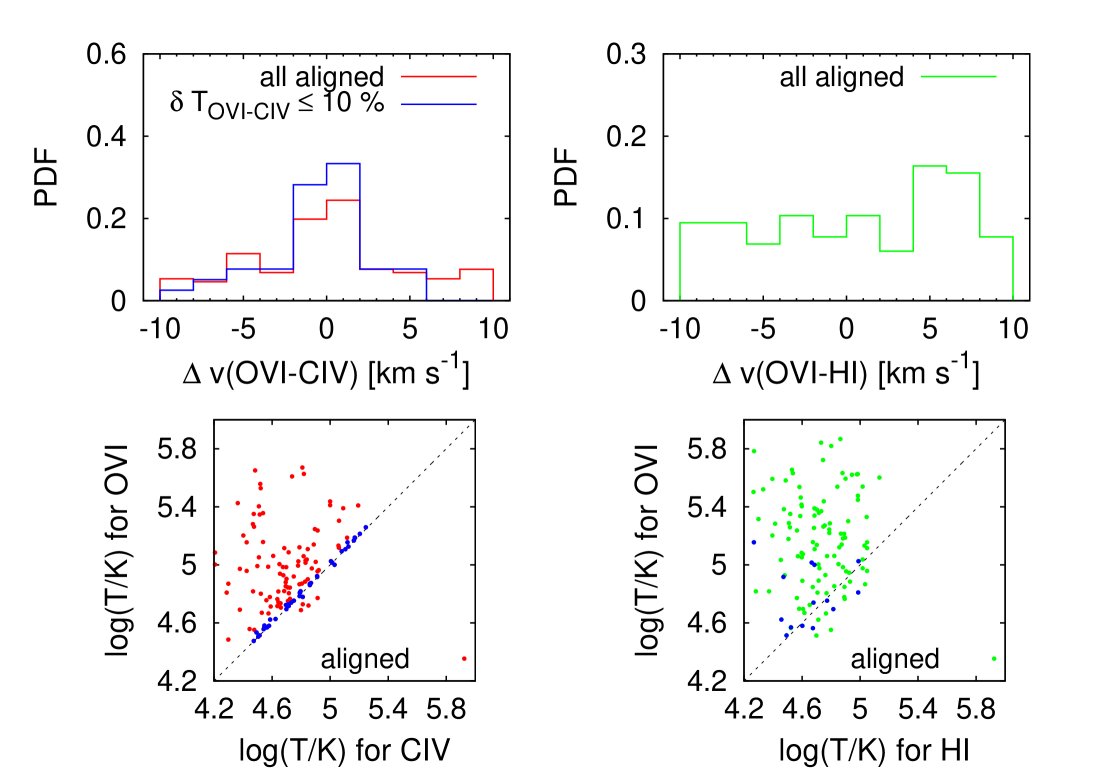
Figure 5.19: Temperatures and velocity offsets of O vi components in high-$z$ OWLS spectra that are well aligned with C iv and H i . Bottom panel: temperature/temperature plots of the well-aligned ($\Delta v=10\leavevmode\nobreak\ \rm km\leavevmode\nobreak\ s^{-1}$) pairs O vi ​​/C iv (left) and O vi ​​/H i (right). Blue dots denote the subsample of O vi ​​/C iv pairs that are aligned in velocity space and that have nearly the same temperature ($\Delta T/T\leq 10$ %). The dashed line indicates the identity of the two quantities. Top panel: the velocity offset distributions are shown. The subsample mentioned above is denoted by the blue line.

O vi ​​/H i aligned absorbers

In general, the temperatures of the O vi components are systematically higher (up to one order of magnitude) than those of the H i components aligned with them (Fig. 5.19, bottom right panel). As said earlier, the velocity alignment might indicate that both ions trace the same overall structure, but possibly arise in physically distinct regions within the host structure with different physical conditions. It is possible, however, that next to the dominating H i absorption component that obviously traces cooler gas there exists an underlying, broad and weak H i component that is physically associated with the warmer O vi absorbing region. For instance, this hot phase could be an interface layer on the surface of a cooler cloud (Boehringer & Hartquist, 1987). In other words, O vi and H i arise in multi-phase gas, where O vi traces the hotter phase while the strong H i traces the cooler one. Considering more complex, multi-component, multi-phase systems, it is to be expected that some broad H i components associated with hot O vi absorbers can be found in spectra with very high S/N. Overall, this result confirms the suggestion of Fox (2011), namely that the alignment between O vi and H i components should not be taken as a proof of single-phase photoionization.

Note that the velocity offset distribution of O vi ​​/H i aligned absorbers (Fig. 5.19, top right panel) has a weak peak at $\approx$ 6 km s^-1 ​​.

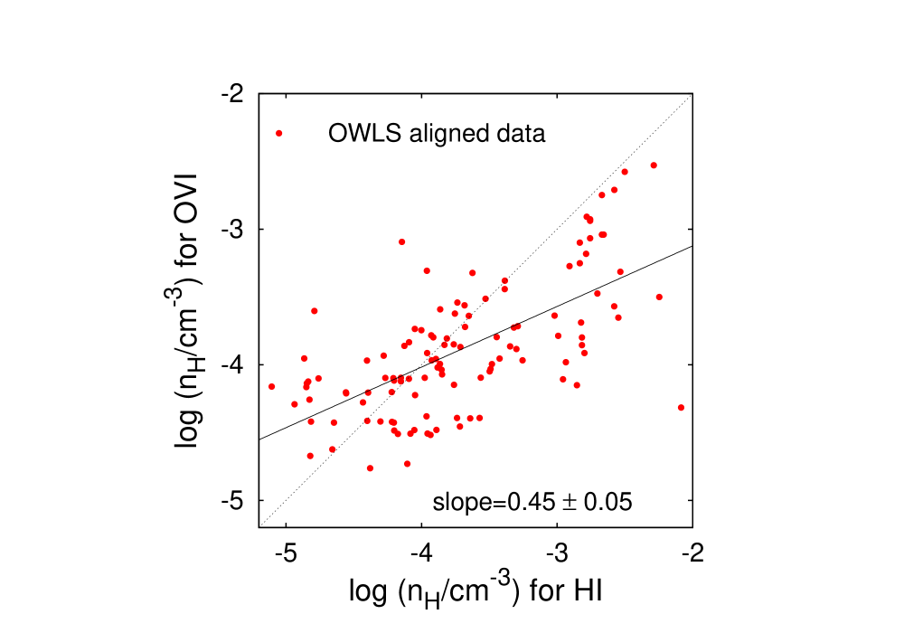
Figure 5.20: Volume density of hydrogen in O vi absorbers and in H i components aligned with them from the hOWLS data. The dashed line indicates the identity of the two quantities.

If the aligned components would reside in single phase, they should exhibit roughly the same volume density of hydrogen, $n_{\rm H}$. However, as seen in Fig. 5.20, this is apparently not the case,‘ suggesting that the aligned O vi and H i components rather arise in different gas phases. The hydrogen density in the O vi absorbers tends to increase slowly (slope $\approx 0.45$) with $n_{\rm H}$ in the aligned H i components. This can be interpreted as an indicator for the existence of multi-phase gas.

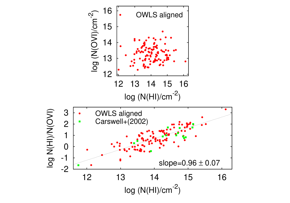
Figure 5.21: Column densities in O vi absorbers and in H i components aligned with them from hOWLS and from observations. Top panel: $N$(O vi ​​) vs. $N$(H i ​​) from hOWLS . Bottom panel: $N$(H i ​​) vs. $N$(H i ​​)/N(O vi ​​). Observational measurements from the O vi ​​/H i sample of Carswell et al. (2002) are plotted with green symbols.

A supplementary comparison of column densities in aligned O vi and H i components is shown in Fig. 5.21. The upper panel shows that there is no correlation between the column densities of O vi and H i ​​, i.e., $N$(O vi ​​) does not change with increasing $N$(H i ​​). A different visualization of this behavior is shown in the lower panel on this figure, where the slope of the distribution $N$(H i ​​)/$N$(O vi ​​) vs. $N$(H i ​​) is close to unity.

O vi ​​/C iv aligned absorbers

Two populations of aligned O vi and C iv components can be distinguished in Fig. 5.19. The one with nearly identical temperatures (difference of $\leq$ 10 per cent) represents about 30 per cent of the whole sample of aligned absorbers (bottom left panel, blue points). The other population contains the rest of the components with a significantly larger scatter in temperatures, suggesting a multi-phase structure of the gas (bottom left panel, red points). The velocity offset distributions (top left panel) for the two populations are similar and do not provide any additional information on the gas phase.

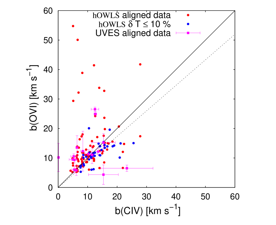
Figure 5.22: Doppler parameters of O vi absorbers and in the H i components aligned with them. The identity of the two quantities is plotted with the solid line, while the dashed line indicates the identity of $b$ under assumption of purely thermal line broadening. The population of aligned absorbers with nearly identical temperatures from the O vi and C iv components is denoted with blue symbols. The observational sample of aligned O vi and C iv components from UVES is shown with violet symbols.

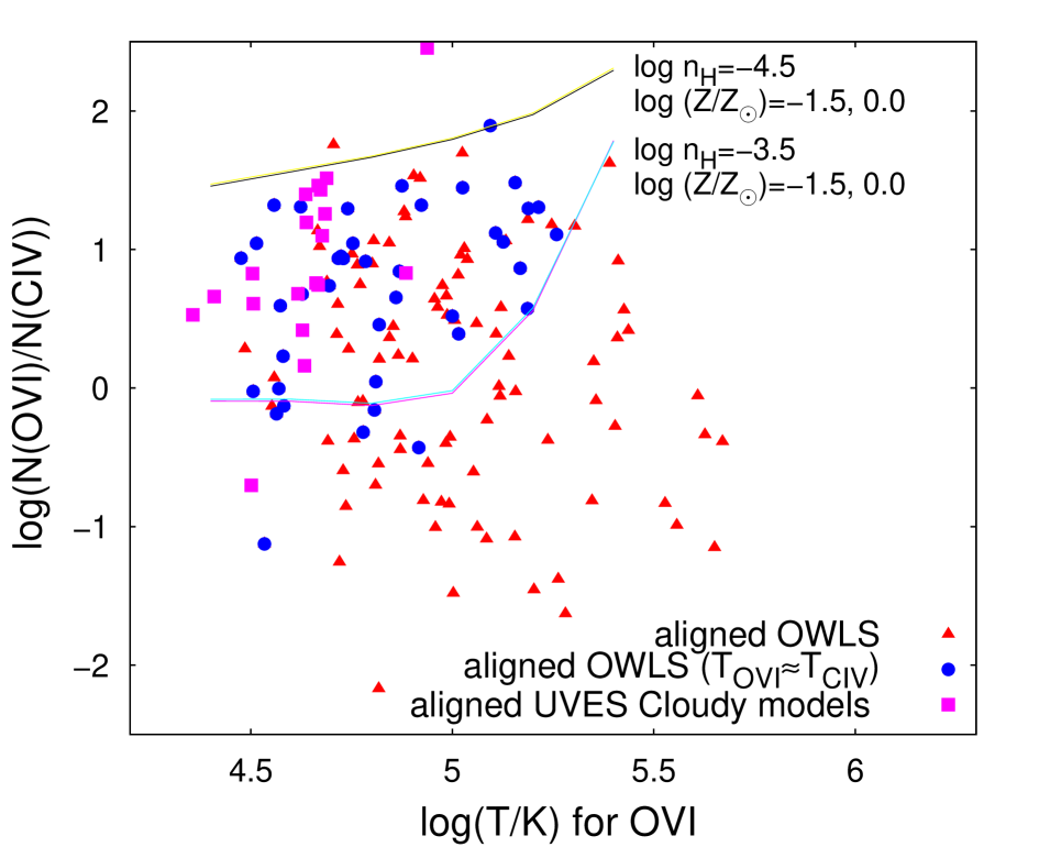
Figure 5.23: Column-density ratio of aligned O vi and C iv components from hOWLS spectra (red triangles) as a function of temperature. The subsample with nearly identical Doppler parameters (temperature differences of $\leq$ 10 per cent) is shown with blue dots. The observational sample of aligned O vi and C iv components from UVES (violet) also are shown; their temperature is obtained from the modeling with Cloudy. Cloudy models for two fixed values of hydrogen density and for two choices of the metallicity (in solar units) are plotted with colored lines.

In an attempt to identify observational criteria to distinguish between the two populations of aligned O vi ​​/C iv absorbers, we compose a comparative diagram of the Doppler parameters of these ions (Fig. 5.22). The identity of the two quantities is plotted with the solid line, while the dashed line indicates the identity of $b$ under assumption of purely thermal line broadening. About 83 per cent of the absorbers with similar temperatures seem to be mostly thermally broadened with comparable $b$-values for O vi and C iv . The Pearson coefficient of correlation between the components of that population is 0.62, which points to a strong correlation. On the other hand, the value for the second population (with different temperatures) is only 0.19, indicating a weak correlation between the components. The likelihood of the coefficients occurring for fully uncorrelated data is $2\times 10^{-5}$ and $0.06$, respectively. The UVES sub-sample of O vi absorbers aligned in velocity with C iv is added in Fig. 5.22 for comparison.

A general conclusion that can be drawn from the Doppler parameters derived for the synthetic O vi ​​/C iv pairs aligned in velocity space is, that, if the O vi absorbers have smaller or equal $b$-values compared to C iv absorbers, 42 per cent have the same temperature and arise in a single gas phase. The remaining 58 per cent of the O vi ​​/C iv pairs have different temperatures and arise in multi-component structures.

To gain further insight into the physical state of O vi absorbers aligned with C iv ​​, we search for a correlation between the O vi ​​/C iv column density ratio and O vi temperature. As can be seen in Fig. 5.23, such a correlation indeed appear to exist for the absorber population with similar temperatures (temperature differences of $\leq$ 10 per cent), as well for the UVES subsample of O vi absorbers aligned with C iv and having the same temperatures as modeled with Cloudy (see Sect. 4.3). We plot the predicted $N$(O vi ​​)/$N$(C iv ​​) ratio as a function of temperature from Cloudy for two fixed metallicities (solar and 0.03 $Z_{\odot}$) and for two choices of the hydrogen density ($\log n_{\rm H}=-3.5$ and $\log n_{\rm H}=-4.5$). Remarkably, $\approx$ 90 per cent of the aligned population with similar temperatures and most of the absorbers from the UVES subsample fall into a narrow density range $-4.5\leq\log n_{\rm H}\leq-3.5$, regardless of the adopted metallicity. We have assumed solar relative abundances of O and C and thus the predicted column density ratio from Cloudy does not depend on the absolute metallicity. The ratio $N$(O vi ​​)/$N$(C iv ​​) for both samples exceeds unity and varies within $\sim 2$ orders of magnitude. The temperature range in these models (see Fig. 5.23) hints at photoionization as the relevant ionizating mechanism in these components.

5.4 Baryon and metal content

As final step of our analysis of high redshift O vi absorbers in the OWLS, we determine the baryon and metal content in these systems. The relative abundances of baryons and metals in different gas phases and their total densities as estimated from the hOWLS are specified in Table 5.2. We find that $\approx$ 38 per cent of the metals in the gas are in the temperature regime $\log T>5\times 10^{4}$ K, whereas the O vi absorbers contribute with $<1$ per cent to the total metal budget. Hence, the conclusion is that O vi absorbers arise in metal-enriched gas, but they do not represent tracers of the main metal reservoirs at high redshift. The baryonic density in O vi systems at high redshift $\Omega_{{\tiny\rm IGM}}^{{\tiny\rm OVI}}$ is less than 1 per cent in the OWLS, in excellent agreement with our estimate from the UVES observations (Chapter 4).

Therefore, our results indicate that high-redshift O vi absorbers neither trace the bulk of the metals at that epoch, nor do they host a significant fraction of the baryonic mass in the Universe.

Table 5.2: Relative mass densities of baryons and metals in hOWLS for different temperature regimes and overdensities.

	Baryons	Metals
log (T/K) $>$ 4.7, $\log\Delta<$2.0	18.30 %	35.53 %
log (T/K) $<$ 4.7, $\log\Delta<$2.0	73.65 %	0.1 %
	$\Omega_{\rm b}(\rm OVI)/\langle\Omega_{\rm b}\rangle$=9.8 $\times 10^{-3}$	$\Omega_{Z}(\rm tot)$= 7.22 $\times 10^{-4}$

5.5 Conclusions

In this chapter, we studied the properties of O vi absorbers at high redshift using artificial absorption spectra obtained from numerical simulations (OWLS). We compared in details the results from OWLS with those from UVES observations presented in the previous chapter. Below we summarize separately the conclusions about the total O vi absorber sample and about the subsample of O vi systems that are aligned in velocity space with the associated H i absorption.

Total O vi sample

• The O vi CDDF obtained from the OWLS O vi absorber sample is in good agreement with that derived from the UVES observations. This implies that the simulations successfully reproduce the statistical properties of metal-enriched, highly ionized gas structures observed in the early Universe. The Doppler parameter distributions obtained from the synthetic and observed O vi spectra suggest that turbulence does not affect significantly the O vi line broadening at high redshift.

• Most of the O vi absorbers from the hOWLS sample populate the region on the density-temperature plane $10^{-5}\leq n_{\rm H}\leq 4\times 10^{-3}$ cm^-3 (overdensities $1.23<\Delta<4.9\times 10^{2}$ at $z=2.5$) and $4\times 10^{4}\leq\rm T\leq 1\times 10^{6}$ K. These (over)densities are roughly one order of magnitude higher than those expected for the diffuse warm-hot WHIM produced by cosmological accretion shocks. They exceed also by $\sim 1$ magnitude the values predicted by the simulations for O vi absorbers at $z=0$. More than 60 per cent of all O vi absorbers at high redshift are found in the temperature regime $10^{5}<\rm T<10^{6}$ K. These relatively high temperatures indicate shock-heated material, as expected for highly-ionized gas expelled by galactic winds and outflows.

• O vi absorbers at high redshift trace metal-enriched material with $\log(Z_{\rm\small{\mbox{O\,{\sc vi}\leavevmode\nobreak\ }}}/Z_{\odot})>-1.5$ and a median value $\approx 0.3\leavevmode\nobreak\ Z_{\odot}$. The median for the low-redshift sample (lOWLS ​​​) is closer to the solar value: $\approx 0.6\leavevmode\nobreak\ Z_{\odot}$. The increase of metallicity from high to low redshifts is consistent with the standard models of cosmic chemical evolution, that predict a rise of the global mean interstellar metallicity in galaxies with time, reaching quasi-solar values at $z=0$.

• The OWLS imply that $\sim$ 38 per cent of the metals in the gas at high redshift are in the temperature regime $\log T>5\times 10^{4}$ K, while O vi absorbers contribute by only $<1$ per cent to the metal budget. We conclude that O vi absorbers arise in metal-enriched gas structures that have a large absorption cross section, but they do not trace the main metal reservoirs. The baryonic density fraction of O vi systems at high redshifts $\Omega_{{\tiny\rm IGM}}^{{\tiny\rm OVI}}$ is less than 1 per cent, so that high-redshift O vi absorbers do not trace the bulk of the baryons either.

Aligned O vi absorbers

• The comparison between non-thermal components of the Doppler parameters in subsamples of well-aligned ($\Delta v\leq 10$ km s^-1 ​​) O vi ​​/H i absorber pairs in the hOWLS and lOWLS spectra shows that both distributions are essentially different. At high redshift, non-thermal broadening contributes poorly to the total width of the O vi lines and thus the Doppler parameter distribution of O vi absorbers can be used (in a statistical sense) to roughly constrain the gas temperature in the absorbers. In contrast, the non-thermal contribution to $b$(O vi ​​) at low redshift is significant, indicating a higher velocity dispersion in O vi absorbing gas structures in the local Universe.

• The temperatures of O vi components are systematically higher, within an order of magnitude, than those of H i components aligned with them in velocity space. This clearly hints at a multiphase gas in the host structure. We speculate that weak, broad H i components, possibly related to the O vi absorbing phase, could be present, but observations with very high S/N ratio would be required to detect them. O vi lines evidently arise in a hot gas phase that is closely aligned in velocity with a cooler phase producing the bulk of the detected H i absorption.

• Two populations of aligned O vi ​​/C iv pairs are identified. One of them contains $\approx 30$ per cent of the whole subsample of aligned O vi ​​/C iv absorbers and displays nearly identical temperatures in the two ions. This population could be well explained by photoionization as the dominating ionization mechanism, with the two ions arising in a single gas phase. The other population, containing $\approx 70$ per cent of the subsample of aligned O vi ​​/C iv ​​, displays significantly different temperatures in O vi and C iv ​​, which suggests a multiphase structure of the gas.

Chapter 6 Conclusions

Our study of high-redshift O vi absorbers presented in the context of this thesis unveils the diverse nature of highly-ionized absorption-line systems in the early Universe. The use of intermediate- and high-resolution optical spectra and cosmological simulations turns out to be a powerful combination that enables us to gain insight into the statistical properties as well as into the physical conditions of these systems. The results from our study that has been described in detail in the previous chapters now can be combined to characterize the complex nature of O vi absorbers at high redshift. The following conclusions can be drawn from our investigations:

• High-redshift O vi absorbers do not have a common origin.

  There are many different indicators for the diverse origin of O vi absorbers at high redshift. Firstly, the spectral analysis of observed and simulated O vi absorbers demonstrates that the kinematics in the absorbers is non-uniform. There are simple O vi absorbers with only one or a few velocity components as well as highly complex O vi systems that span a large velocity range with a large number of subcomponents. Secondly, the missing velocity alignment between O vi ​​, C iv ​​, and H i ​​, seen in a large fraction of the O vi absorbers, and the temperature differences of aligned O vi ​​/H i and O vi ​​/C iv pairs, found in the synthetic spectra, both indicate multi-phase gas that contains hotter and cooler gas regions that are spatially separated from each other, and that are traced by different ions. Other absorbers, however, do not show such a velocity signature, indicating a different spatial alignment of the different gas phases. Thirdly, the small Doppler parameters of some of the O vi absorbers indicate that they have temperatures less that $10^{5}$ K and are photoionized, while collisional ionization appears to dominate in other O vi systems. Therefore, the physical conditions, that govern the ionization state of these systems, appear to vary substantially among the O vi absorber population, indicating that they arise in a wide variety of environments. Fourthly, the results that we obtain for the gas densities and absorption path lengths of the O vi absorbers demonstrate that measurable O vi absorption occurs both in large-scale structures of several hundred kpc and in small-scale structures with sizes on the order of a few parsec.

  The physical pictures emerging from this facts is that the observed O vi absorption traces a transition gas phase of temperature $T\sim 10^{5}$ K which is characteristic for many small-and large-scale gaseous environments in the Universe. As discussed by Fox (2011), the most plausible scenario is that many O vi absorbers arise in conductive, turbulent, or shocked boundary layers between warm ($\sim 10^{4}$ K) and hot ($\sim 10^{6}$ K) gas, supporting the unified cooling-flow model proposed by (Heckman et al., 2002). Thus the O vi absorption in such transition regions would be a natural result of the multi-phase nature of the circumgalactic and intergalactic gas. Including the photoionized systems, O vi absorbers possibly trace galactic winds and outflows, transition layers between infalling intergalactic gas and hot coronal halo gas, but also photoionized metal enriched gas patches that had been injected previously into the intergalactic filaments, and gas with transition-temperature has been stripped by galaxy interactions.

  The summarizing conclusion is that O vi reflects, like no other ion, the extreme physical and spatial complexity of gas in the circulgalactic and intergalactic environment of galaxies at low and high redshift. The interpretation of O vi absorption in high-redshift QSO spectra thus requires a careful case-by-case analysis including other intermediate and high ions and a detailed comparison of the velocity-component structure in the different ions, using both, cosmological simulations and observations.

• High-redshift O vi absorbers neither trace the bulk of the baryons, nor do they trace the bulk of the metals at that epoch.

  The analyzed UVES and OWLS samples both clearly indicate that the highly-ionized gas as traced by intervening O vi absorbers at high redshift cannot host a significant fraction of the baryons and metals at $z=2-3$. Instead, our results imply that the baryon- and metal-content of these absorbers is expected to be less than 1 percent of the total mass-density of baryons and metals at that epoch. Therefore, our results contradict to some previous O vi studies wherein the O vi ion is identified as an important tracer of the cosmic baryons and metals in the early Universe (e.g., Bergeron & Herbert-Fort, 2005). On the other hand, our results are in excellent agreement with more recent results of other groups, e.g., Muzahid et al. (2012), that find similar (low) O vi mass/metal densities from their analysis of high-redshift high-ion absorbers.

• The physical conditions in O vi absorbers change over the cosmic time scale.

  The comparison between O vi absorbers at low and high redshift from our study and others (Tepper-García et al., 2011; Muzahid et al., 2012; Tripp et al., 2008) unveils interesting aspects on the time-evolution of the O vi absorbing gas in the Universe. Clearly, the physical properties of O vi absorbers at high redshift are different from the low redshift O vi absorber population. The OWLS imply that the gas density in the O vi absorbers at high redshift is (on average) by one order of magnitude higher than at low redshift, while the smoothed metallicity is twice less. Non-thermal line-broadening mechanisms appears to be irrelevant for high redshift O vi systems, while they are important for O vi absorbers at low redshift, possibly indicating higher turbulence in the absorbing region, caused, for instance, by large-scale accretion shocks. Again, this indicates that O vi does not trace characteristic regions in the circumgalactic and intergalactic medium in the Universe, but rather a characteristic gas phase which results from the ambient physical conditions that govern the ionization structure in the absorbers. Thus, the observed frequency of O vi absorption in QSO spectra at different epochs is conditioned by the absorption-cross section of the widespread gas with transition temperature in the course of the on-going structure evolution of the Universe from high to low redshift.

• The kinematic and physical properties of high-redshift O vi absorbers suggest an inhomogeneous metal enrichment of the IGM.

  As mentioned above, the kinematic displacement between O vi ​​, C iv ​​, H i and other ions observed in the optical and the synthetic spectra, considered together with the temperature constraints for the different ions obtained from simulations, indicate that the hosts of O vi absorbers at high redshift represent multi-phase gas absorbers with substantial substructure. Moreover, the OWLS further indicate that the metals are not uniformly distributed along the absorber host, but are concentrated in confined regions (i.e., O vi absorbing regions) that exhibit a substantially higher local metallicity than in the surrounding medium. Such a scenario is supported by the observational study of Schaye et al. (2007), who argued that the intergalactic metals were transported into the IGM through galactic winds in the form of highly-enriched gas patches (metal “bullets”) that do not (fully) mix with the ambient hydrogen gas. A similar conclusion was drawn by Tepper-García et al. (2011), who studied O vi absorbers at low redshift using OWLS. Therefore, we point out that derived metallicities in high redshift intergalactic and circumgalactic medium from observational O vi ​​/H i ratios, without knowledge of the 3D structure of the absorbing gas phases, are afflicted with large systematic uncertainties.

Our summarizing conclusion is that the O vi ion is indeed an important species that provides substantial information on the physical conditions in multi-phase gas around galaxies, but our understanding of the complex interplay between the different gas phases will remain incomplete if derived from O vi data alone. Therefore, future studies of other tracers of hot gas, such as the broad-line absorbers (e.g., Richter et al., 2006) and Ne viii (e.g., Savage et al., 2005), together with high-resolution cosmological simulations and simulations of galaxy formation, will substantially improve our understanding of the distribution and physical conditions of highly-ionized gas in the circumgalactic and intergalactic medium and its role in the ongoing structure formation in the Universe.

Appendix A Details of OVI systems from the UVES sample

A.1 Basic information about the sample

Table A.1: The selected sample of O vi absorbers from the UVES survey. Columns 1-3 give the designations of the associated QSO, its emmision redshift and proximity redshifts, correspondingly. Column 4 gives the absorption lenght of each QSO. Columns 5 and 6 contain information about the redshift of the O vi absorbers in each QSO sightline and specify their number of components.

QSO				O vi absorption systems
Name	$z_{\text{em}}$	$z_{\text{prox}}$	$X$	$z_{\text{abs}}$	category	comp.
HE 1122-1648	2.404	2.387	1.60312	2.4193a	2	3
HE 1347-2457	2.609	2.592	1.76352	2.1162	0	2
				2.2347	2	3
				2.3287	1	4
				2.5745	2	1
HE 2217-2818	2.413	2.396	1.60999	2.0747	0	1
				2.0755	2	1
				2.1806	2	2
				2.1818	2	3
HE 2347-4342	2.874	2.857	1.97706	2.6498	1	3
				2.7105	0	1
				2.7119	0	2
				2.8625a	2	3
				2.8911a	2	8
				2.8975a	2	15
J 2233-606	2.250	2.233	1.48524	2.1982	1	4
				2.2045	1	6
				2.2099	2	4
PKS 0237-233	2.223	2.206	1.46482	2.2028	1	2
				2.2135a	1	3
				2.2364a	1	5
				2.2378a	2	3
PKS 0329-255	2.704	2.687	1.83925	2.4252	1	3
				2.6494	2	2
				2.6610	2	2
				2.7089	1	12
PKS 2126-158	3.279	3.262	2.3164	2.9074	0	1
Q 0002-422	2.767	2.750	1.88999	2.4640	1	10
				2.5395	0	1
				2.7011	0	1
Q 0055-269	3.655	3.638	2.64486	3.6015	0	2
Q 0109-3518	2.405	2.388	1.60378	2.4012a	1	1
Q 0122-380	2.193	2.176	1.4422	2.0626	2	1
Q 0329-385	2.434	2.417	1.62627	2.3521	1	1
				2.3639	2	3
				2.3737	2	2
Q 0420-388	3.116	3.099	2.17793	3.0872	1	7
Q 0453-423	2.658	2.641	1.80252	2.3978	0	8
				2.6362	1	4
				2.6405	2	2

^a Associated O vi systems. The rest are intervening O vi systems.

A.2 OVI/HI column density ratio

Table A.2: O vi ​​/H i column density ratio of the absorbers from the UVES sample.

Absorption systems
QSO name	$z_{\text{abs}}$(comp.)	N(O vi ​​)/N(H i ​​)
HE 1122-1648	2.4193(3)	2.48 ($+0.125895\atop-0.119031$)
HE 1347-2457	2.1162(2)	1.36 ($+2.115240\atop-0.629865$)
	2.2347(3)	0.30 ($+0.038379\atop-0.028066$)
	2.3287(2)	0.01 ($+0.006326\atop-0.002888$)
	2.5745(1)	0.04 ($+0.002690\atop-0.002534$)
HE 2217-2818	2.0747(1)	0.17 ($+0.026903\atop-0.027346$)
	2.0755(1)	1.32 ($0.232336\atop-0.239987$)
	2.1818(5)	0.01 ($+0.003321\atop-0.002649$)
HE 2347-4342	2.6498(3)	0.05 ($+0.004540\atop-0.004138$)
	2.7105(1)/2.7119(2)	0.09 ($+0.024777\atop-0.020612$)
	2.8625(3)	0.20 ($+0.032029\atop-0.023465$)
	2.8911(8)	16.29 ($+2.861322\atop-4.189452$)
	2.8975(15)	0.23 ($+0.039362\atop-0.030874$)
J 2233-606	2.1982(4)	42.52 ($+9.125267\atop-7.319435$)
	2.2045(7)	9.45 ($+13.220907\atop-3.972540$)
	2.2099(4)	69.29 ($+65.221252\atop-30.303299$)
PKS 0237-233	2.2028(2)	0.004 ($+0.021299\atop-0.002665$)
	2.2135(3)	0.25 ($+0.166593\atop-0.052706$)
	2.2364(8)	1.16 ($+0.473380\atop-0.417801$)
PKS 0329-255	2.4252(3)	0.02 ($+0.004236\atop-0.003700$)
	2.6494(2)	0.04 ($+0.026871\atop-0.015146$)
	2.6610(2)	0.13 ($+0.015739\atop-0.013707$)
	2.7089(11)	1.48 ($+2.164616\atop-0.946345$)
PKS 2126-158	2.9074(1)	0.002 ($+0.000177\atop-0.000160$)
Q 0002-422	2.4640(10)	0.007 ($+0.000952\atop-0.000719$)
	2.5395(1)	0.14 ($+0.083378\atop-0.072789$)
	2.7011(1)	0.071 ($+0.008505\atop-0.007606$)
Q 0055-269	3.6015(2)	0.02 ($+0.001966\atop-0.001821$)
Q 0109-3518	2.4012(1)	0.11 ($+0.013681\atop-0.012222$)
Q 0122-380	2.0626(1)	3.96 ($+1.747881\atop-1.255565$)
Q 0329-385	2.3521(1)	5.94 ($+1.304771\atop-1.143078$)
	2.3639(3)	0.11 ($+0.095031\atop-0.053387$)
	2.3737(2)	0.086 ($+0.015742\atop-0.013308$)
Q 0420-388	3.0872(7)	0.00002 ($+0.000001\atop-0.000001$)
Q 0453-423	2.3978(8)	0.75 ($+0.183549\atop-0.201516$)
	2.6362(4)	0.096 ($+0.018013\atop-0.015103$)
	2.6403(2)	0.04 ($+0.024809\atop-0.039332$)

A.3 Error estimates

$$N_{tot}(O\,\text{\sc vi})=\displaystyle{\sum_{c}N_{c}(O\,\text{\sc vi})}$$

$$\sigma^{+}_{tot}(N(O\,\text{\sc vi}))=\sqrt{\displaystyle{\sum_{c}\sigma^{+}_{c}(N(O\,\text{\sc vi}))^{2}}}$$

$$\sigma^{-}_{tot}(N(O\,\text{\sc vi}))=\sqrt{\displaystyle{\sum_{c}\sigma^{-}_{c}(N(O\,\text{\sc vi}))^{2}}}$$

$N_{c}(O\,\text{\sc vi})$ and $\sigma_{c}(N(O\,\text{\sc vi}))$ are the $\log$ of the column densities and their errors for each component for a given system, derived form the fit. Similar is for H i .

$$\sigma^{+}_{c}(N(O\,\text{\sc vi}))=(10^{\sigma_{c}(N(O\,\text{\sc vi}))}-1)\times 10^{N_{c}(O\,\text{\sc vi})}$$

$$\sigma^{-}_{c}(N(O\,\text{\sc vi}))=(1-10^{-\sigma_{c}(N(O\,\text{\sc vi}))})\times 10^{N_{c}(O\,\text{\sc vi})}$$

A.4 Fitting results

Table A.3: Voigt Profile parameters of the absorption lines (HE 1122-1648).

$z=2.419294$
$\rm Ion$	$z$	$\rm Error$	log[N (cm-2)]	$\rm Error$	$b$ [km s-1 ]	$\rm Error$
O VI	2.419290	0.000001	13.992	0.010	9.49	0.18
O VI	2.419631	0.000030	13.499	0.030	27.84	2.22
O VI	2.419846	0.000006	12.837	0.087	7.58	1.30
C IV	2.419229	0.000007	11.537	0.054	4.96	1.24
N V	2.419232	0.000010	12.127	0.027	17.10	1.32
H I	2.419248	0.000004	13.650	0.009	28.60	0.19
H I	2.419724	0.000020	13.013	0.040	31.50	1.66

Table A.4: Voigt Profile parameters of the absorption lines (HE 1347-2457).

$z=2.574499$
$\rm Ion$	$z$	$\rm Error$	log [N (cm-2)]	$\rm Error$	$b$ [km s-1 ]	$\rm Error$
O VI	2.574503	0.000006	13.540	0.011	26.53	0.74
C IV	2.574516	0.000028	13.122	0.172	12.50	1.29
C IV	2.574586	0.000006	12.758	0.162	3.26	1.51
C IV	2.574808	0.000279	12.249	0.695	18.84	21.96
C IV	2.574408	0.000005	13.033	0.089	3.91	0.72
C III	2.574512	0.000004	14.504	0.163	7.72	0.48
C III	2.574735	0.000106	12.528	0.358	13.22	6.82
C II	2.574592	0.000002	12.921	0.019	3.65	0.43
C II	2.574415	0.000006	12.715	0.035	6.36	0.84
S iIV	2.574417	0.000002	12.268	0.015	3.59	0.33
Si IV	2.574578	0.000003	12.097	0.023	4.38	0.56
Si III	2.574439	0.000001	12.393	0.010	4.15	0.19
Si III	2.574600	0.000002	12.265	0.012	5.25	0.29
Si II	2.574409	0.000003	11.749	0.026	3.76	0.64
Si II	2.574587	0.000003	11.796	0.022	2.96	0.60
H I	2.574508	0.000001	14.898	0.015	15.50	0.15
H I	2.574964	0.000037	12.482	0.115	14.90	3.16
$z=2.116204$
O VI	2.116207	0.000008	14.275	0.190	8.69	2.46
O VI	2.116279	0.000146	13.901	0.653	16.18	6.90
C IV	2.115819	0.000034	11.870	0.185	9.73	5.40
C IV	2.116208	0.000002	13.205	0.074	6.24	0.60
C IV	2.116578	0.000083	12.363	0.205	23.27	11.26
C IV	2.116148	0.000028	12.925	0.152	13.09	1.46
C IV	2.116775	0.000017	11.914	0.349	6.33	4.46
N V	2.116089	0.000119	12.476	0.556	11.09	9.50
N V	2.116211	0.000013	12.673	0.344	5.76	2.55
H I	2.116222	0.000010	13.791	0.072	17.63	1.48
H I	2.116318	0.000116	14.131	0.122	59.61	9.27
$z=2.328666$
O VI	2.328914	0.000029	13.899	0.168	10.04	1.86
O VI	2.328666	0.000017	14.141	0.023	49.81	2.03
O VI	2.328674	0.000031	14.310	0.193	13.44	1.05
O VI	2.328689	0.000031	13.592	0.696	5.32	6.41
C IV	2.328908	0.000002	13.807	0.025	7.24	0.38
C IV	2.329536	0.000005	13.106	0.064	7.16	0.71
C IV	2.329220	0.000012	13.445	0.048	19.38	2.35
C IV	2.329691	0.000012	12.889	0.074	8.24	1.29
C IV	2.329971	0.000019	12.030	0.090	9.50	3.34
C IV	2.328659	0.000015	13.666	0.033	18.09	1.88
C IV	2.328610	0.000003	13.266	0.111	7.06	0.84
C IV	2.328130	0.000050	11.965	0.174	14.31	6.25
C IV	2.329040	0.000010	12.833	0.182	4.65	1.49
C III	2.329584	0.000012	13.664	0.047	15.43	1.37
C III	2.328997	0.000028	14.040	0.023	37.31	1.71
C III	2.328613	0.000017	13.223	0.114	9.67	1.81
C III	2.330013	0.000021	11.779	0.169	4.23	3.85
Si IV	2.328610	0.000006	12.285	0.025	10.62	1.00
Si IV	2.328946	0.000003	12.622	0.014	8.91	0.43
Si IV	2.329227	0.000007	12.183	0.035	9.21	1.15
Si IV	2.329534	0.000005	12.469	0.044	5.91	0.58
Si IV	2.329692	0.000025	11.965	0.139	7.95	2.98
Si III	2.328624	0.000013	11.854	0.058	9.99	1.46
Si III	2.329236	0.000004	12.084	0.031	8.92	0.92
Si III	2.328998	0.000003	12.419	0.022	7.18	0.56
Si III	2.328820	0.000015	11.562	0.192	6.29	3.16
Si III	2.329587	0.000006	12.476	0.029	14.05	0.95
Si III	2.329558	0.000004	11.996	0.098	4.20	1.00
H I	2.327651	0.000013	14.308	0.035	22.45	1.19
H I	2.328334	0.000245	14.287	0.511	30.24	16.12
H I	2.328981	0.000023	16.484	0.048	29.05	1.77
H I	2.329538	0.000044	16.018	0.088	27.74	1.60
H I	2.330345	0.000953	13.072	0.906	73.95	130.14
H I	2.331558	0.000229	12.432	0.784	39.55	23.82
$z=2.234653$
O VI	2.234886	0.000027	14.094	0.033	39.70	2.01
O VI	2.234652	0.000013	13.683	0.069	11.32	1.50
O VI	2.234447	0.000064	12.878	0.417	10.21	5.61
C IV	2.234972	0.000007	12.845	0.019	17.43	0.94
C IV	2.234642	0.000006	12.584	0.041	10.27	1.07
H I	2.234600	0.000008	14.782	0.012	47.28	0.61

Table A.5: Voigt Profile parameters of the absorption lines (HE 2217-2818)

$z=2.074720,\leavevmode\nobreak\ \leavevmode\nobreak\ \leavevmode\nobreak\ \leavevmode\nobreak\ 2.075462$
O VI	2.075464	0.000004	14.253	0.029	12.15	0.55
O VI	2.074719	0.000010	14.194	0.042	15.02	1.40
C IV	2.075352	0.000049	12.134	0.323	20.40	6.62
C IV	2.074687	0.000011	12.674	0.054	10.18	0.99
C IV	2.074835	0.000010	12.408	0.099	7.47	1.11
C IV	2.075398	0.000003	12.737	0.082	10.09	0.96
H I	2.074772	0.000008	14.954	0.021	28.52	1.11
H I	2.075474	0.000010	14.083	0.036	26.74	1.21
H I	2.076023	0.000312	13.157	0.329	68.76	43.98
H I	2.074324	0.000276	13.272	0.625	32.08	14.41
$z=2.181784$
O VI	2.180448	0.000016	12.606	0.196	3.81	3.60
O VI	2.180648	0.000016	13.828	0.023	34.36	1.84
O VI	2.181398	0.000014	13.199	0.065	11.75	2.07
O VI	2.181990	0.000017	13.880	0.028	28.87	1.78
O VI	2.181783	0.000008	12.956	0.131	4.20	2.20
C IV	2.180838	0.000003	12.413	0.078	4.40	0.82
C IV	2.180748	0.000003	13.411	0.015	15.24	0.28
C IV	2.181723	0.000006	12.343	0.120	7.02	1.06
C IV	2.181168	0.000007	11.855	0.143	5.16	1.92
C IV	2.180414	0.000012	11.959	0.068	9.11	1.75
C IV	2.181892	0.000056	12.227	0.282	15.53	6.79
C IV	2.181419	0.000469	11.842	0.813	42.40	81.93
C II	2.180644	0.000010	11.933	0.114	3.76	2.24
C II	2.180817	0.000004	12.670	0.023	8.04	0.69
Si IV	2.180838	0.000002	12.351	0.049	4.26	0.49
Si IV	2.180741	0.000006	12.695	0.024	12.35	0.34
Si IV	2.181179	0.000013	11.128	0.113	3.64	2.62
Si IV	2.181813	0.000022	10.876	0.204	3.38	4.79
Si III	2.180755	0.000009	12.880	0.043	12.61	0.52
Si III	2.180853	0.000002	12.591	0.057	4.97	0.59
Si II	2.180812	0.000012	11.643	0.105	8.28	1.48
Si II	2.180619	0.000043	11.456	0.165	12.70	4.15
Mg II	2.180818	0.000007	11.546	0.043	7.47	1.13
Mg II	2.180619	0.000015	11.257	0.175	6.57	3.03
Mg II	2.180434	0.000042	11.148	0.196	10.22	5.04
H I	2.179567	0.000216	12.021	0.420	26.24	17.03
H I	2.179936	0.000038	12.630	0.233	17.02	5.55
H I	2.180784	0.000009	16.075	0.082	27.86	0.78
H I	2.181350	0.000073	14.901	0.070	52.64	2.63
H I	2.182075	0.000012	13.660	0.059	16.88	1.04

Table A.6: Voigt Profile parameters of the absorption lines (HE 2347-4342).

$z=2.649846$
$\rm Ion$	$z$	$\rm Error$	log [N (cm-2)]	$\rm Error$	$b$ [km s-1 ]	$\rm Error$
O VI	2.649554	0.000003	13.538	0.032	11.40	0.57
O VI	2.649849	0.000002	13.486	0.011	6.34	0.27
O VI	2.649202	0.000006	13.172	0.082	10.18	1.16
C IV	2.649072	0.000014	12.414	0.036	17.29	1.87
C IV	2.649486	0.000010	12.049	0.058	6.46	1.42
C IV	2.649800	0.000006	12.223	0.033	6.15	0.83
H I	2.647204	0.000019	12.646	0.053	17.24	1.62
H I	2.647789	0.000023	13.779	0.171	14.67	2.26
H I	2.648030	0.000016	14.577	0.030	26.81	0.65
H I	2.648996	0.000007	15.025	0.014	37.93	0.31
$z=2.710477,\leavevmode\nobreak\ \leavevmode\nobreak\ \leavevmode\nobreak\ \leavevmode\nobreak\ 2.711919$
O VI	2.710474	0.000006	12.732	0.049	7.53	0.99
O VI	2.711482	0.000008	13.376	0.100	13.53	1.34
O VI	2.711921	0.000004	13.502	0.051	10.56	0.84
C IV	2.711910	0.000007	12.040	0.049	5.29	1.01
C IV	2.712238	0.000027	12.076	0.103	13.04	4.05
C IV	2.712441	0.000578	11.132	1.145	0.70	152.69
H I	2.713043	0.000028	13.820	0.036	27.08	1.40
H I	2.711870	0.000159	14.194	0.223	40.26	9.96
H I	2.712348	0.000020	14.617	0.079	29.31	1.37
H I	2.711071	0.000077	13.901	0.094	45.19	3.30
$z=2.862508$
O VI	2.861969	0.000060	12.791	0.110	23.69	7.22
O VI	2.862512	0.000013	13.496	0.050	13.96	1.53
O VI	2.862768	0.000042	12.574	0.323	8.34	4.07
C IV	2.862398	0.000012	12.575	0.223	7.81	1.79
C IV	2.862464	0.000091	12.456	0.408	16.97	5.38
C IV	2.862681	0.000016	12.301	0.259	6.82	2.37
C III	2.862395	0.000003	12.595	0.013	9.17	0.39
C III	2.862689	0.000005	12.175	0.026	5.99	0.65
H I	2.861969	0.000051	12.277	0.364	16.81	5.81
H I	2.862347	0.000004	14.273	0.006	36.04	0.15
H I	2.862668	0.000006	13.240	0.034	15.50	0.65
$z=2.891062$
O VI	2.889387	0.000047	11.779	0.627	3.86	9.71
O VI	2.890273	0.000001	14.550	0.010	12.05	0.23
O VI	2.891641	0.000003	15.122	0.039	13.45	0.72
O VI	2.889784	0.000003	13.731	0.034	11.45	0.55
O VI	2.892214	0.000003	14.059	0.027	7.81	0.41
O VI	2.891278	0.000095	14.411	0.068	71.34	10.30
O VI	2.891056	0.000003	15.483	0.053	13.73	0.44
O VI	2.892465	0.000009	13.751	0.047	11.38	0.98
N V	2.889749	0.000065	11.888	0.212	12.93	7.71
N V	2.890236	0.000011	12.790	0.033	14.06	1.42
N V	2.890867	0.000010	13.242	0.092	6.34	0.76
N V	2.891004	0.000011	13.542	0.076	20.83	2.04
N V	2.891027	0.000005	13.722	0.052	7.56	0.56
N V	2.891601	0.000001	13.934	0.010	10.17	0.14
N V	2.892171	0.000016	12.315	0.111	7.08	1.83
N V	2.892445	0.000057	12.154	0.177	13.14	6.76
C IV	2.888361	0.000015	12.195	0.049	12.03	1.84
C IV	2.889388	0.000015	12.330	0.044	13.75	1.76
C IV	2.890233	0.000014	12.402	0.040	14.06	1.68
C IV	2.890973	0.000001	13.654	0.006	13.31	0.15
C IV	2.891600	0.000001	13.869	0.006	9.25	0.10
C IV	2.892056	0.000206	12.442	0.163	50.85	20.47
C IV	2.892166	0.000023	11.722	0.218	5.62	3.79
H I	2.889376	0.000064	13.769	0.161	23.60	2.05
H I	2.889432	0.000072	12.375	1.445	11.55	9.77
H I	2.889645	0.000041	13.263	0.335	16.99	2.82
H I	2.889845	0.000076	13.637	0.021	51.68	3.48
H I	2.890765	0.000005	13.312	0.061	15.54	0.80
H I	2.891202	0.000022	14.137	0.029	40.03	2.25
H I	2.891712	0.000109	13.174	0.435	17.08	7.41
H I	2.891911	0.000034	13.051	0.448	12.65	2.40
H I	2.892218	0.000084	13.070	0.125	39.38	7.75
H I	2.893180	0.000192	12.012	0.268	34.87	12.91
$z=2.897458$
O VI	2.897446	0.000011	10.370	1.400	17.59	0.84
O VI	2.896074	0.000003	13.007	0.036	5.22	0.60
O VI	2.898437	0.000009	14.269	0.046	12.54	0.51
O VI	2.899937	0.000004	14.268	0.027	11.68	0.64
O VI	2.899635	0.000004	13.893	0.031	8.31	0.62
O VI	2.900676	0.000005	14.206	0.030	14.20	0.73
O VI	2.901285	0.000048	14.802	0.133	24.27	2.33
O VI	2.901645	0.000026	13.954	0.473	10.97	4.90
O VI	2.900257	0.000011	13.935	0.062	14.76	1.92
O VI	2.898493	0.000006	13.639	0.129	4.82	1.24
O VI	2.897475	0.000006	15.477	0.089	24.18	1.68
O VI	2.896836	0.000163	13.853	0.267	33.90	9.54
O VI	2.898096	0.000007	13.324	0.134	6.23	1.32
O VI	2.898837	0.000056	13.469	0.175	20.94	8.49
O VI	2.899340	0.000028	13.087	0.181	11.61	4.77
N V	2.896028	0.000013	11.974	0.090	4.20	2.16
N V	2.896851	0.000265	12.663	0.849	15.31	9.81
N V	2.897129	0.000026	14.017	0.311	7.29	1.41
N V	2.897210	0.000016	14.519	0.152	6.31	1.26
N V	2.897279	0.000211	13.773	0.451	16.39	13.51
N V	2.897613	0.000137	13.867	0.476	18.75	4.07
N V	2.897646	0.000008	13.715	0.195	8.99	1.30
N V	2.898292	0.000058	12.711	0.346	8.07	3.02
N V	2.898440	0.000014	13.268	0.094	7.48	0.86
N V	2.902997	0.000017	12.359	0.088	8.32	2.22
N V	2.902345	0.000007	13.105	0.023	13.45	0.64
N V	2.901373	0.000019	12.738	0.116	13.00	4.24
N V	2.901643	0.000021	12.460	0.146	7.82	2.07
N V	2.901063	0.000041	12.090	0.239	8.09	3.98
N V	2.902714	0.000002	13.294	0.016	8.68	0.36
N V	2.904084	0.000006	13.360	0.012	21.74	0.65
C IV	2.896021	0.000002	12.888	0.014	4.62	0.24
C IV	2.896309	0.000039	12.054	0.194	12.09	7.47
C IV	2.896544	0.000015	11.900	0.219	4.26	2.93
C IV	2.896793	0.000003	13.063	0.033	6.29	0.40
C IV	2.897207	0.000010	15.131	0.126	10.46	0.26
C IV	2.897613	0.000013	14.628	0.049	13.45	0.66
C IV	2.897911	0.001253	12.812	0.984	45.61	56.30
C IV	2.898361	0.000025	13.685	0.192	7.85	0.86
C IV	2.898450	0.000011	13.755	0.158	6.50	0.47
C IV	2.904092	0.000003	13.652	0.005	19.06	0.26
C IV	2.902904	0.000065	12.927	0.139	19.71	4.18
C IV	2.902697	0.000001	13.461	0.036	8.84	0.35
C IV	2.902356	0.000003	13.342	0.010	12.99	0.27
C IV	2.901045	0.000017	12.176	0.110	7.28	1.76
C IV	2.901341	0.000025	12.436	0.145	12.68	4.87
C IV	2.901634	0.000048	12.088	0.229	9.87	4.29
H I	2.896018	0.000011	12.093	0.028	15.35	1.26
H I	2.897031	0.000004	13.650	0.014	14.60	0.25
H I	2.897227	0.000005	13.515	0.018	38.07	0.74
H I	2.897323	0.000003	13.577	0.016	12.72	0.26
H I	2.898435	0.000002	13.047	0.004	18.89	0.22
H I	2.899817	0.000003	13.745	0.011	28.68	0.32
H I	2.901276	0.000013	14.709	0.009	75.37	1.14
H I	2.902645	0.000001	15.990	0.005	32.55	0.16
H I	2.904100	0.000001	15.983	0.006	29.72	0.08

Table A.7: Voigt Profile parameters of the absorption lines (J 2233-606).

$z=2.198231$
$\rm Ion$	$z$	$\rm Error$	log [N (cm-2)]	$\rm Error$	$b$ [km s-1 ]	$\rm Error$
O VI	2.198320	0.000022	15.258	0.088	27.40	1.78
O VI	2.197800	0.000023	14.314	0.140	11.79	4.08
O VI	2.197558	0.000055	13.223	0.701	7.15	8.93
O VI	2.197311	0.000036	13.919	0.108	18.66	4.54
N V	2.198264	0.000041	14.068	0.074	29.94	2.43
N V	2.197900	0.000029	13.647	0.173	21.41	2.65
N V	2.197378	0.000088	13.138	0.127	35.05	8.81
N V	2.198168	0.000021	12.631	0.467	8.75	5.23
C IV	2.197304	0.000050	12.651	0.078	32.64	7.30
C IV	2.197882	0.000044	13.177	0.226	15.64	2.70
C IV	2.198179	0.000014	13.756	0.083	19.25	3.28
C IV	2.198506	0.000040	12.882	0.231	13.78	3.73
C IV	2.198884	0.000022	12.319	0.095	11.83	3.41
H I	2.198144	0.000004	13.680	0.005	39.79	0.57
H I	2.197173	0.000041	12.045	0.103	20.23	5.89
H I	2.198931	0.000065	11.915	0.180	19.77	8.91
$z=2.204508$
O VI	2.204855	0.000489	14.717	0.659	68.64	18.58
O VI	2.204495	0.000021	13.863	0.142	14.82	4.74
O VI	2.205754	0.000502	14.912	0.459	77.93	37.64
O VI	2.207318	0.000066	14.701	0.085	63.46	9.08
O VI	2.208613	0.000098	13.982	0.115	49.39	10.74
O VI	2.203191	0.000040	13.045	0.173	10.99	5.91
N V	2.207125	0.000074	13.840	0.047	89.43	6.10
N V	2.204795	0.000463	13.718	0.263	108.18	20.39
N V	2.204491	0.000011	12.583	0.084	10.53	1.96
N V	2.205954	0.000021	13.132	0.128	26.71	3.53
N V	2.205256	0.000047	13.579	0.270	55.99	10.87
C IV	2.203913	0.000032	12.430	0.100	16.38	4.88
C IV	2.204459	0.000011	13.046	0.110	12.63	1.56
C IV	2.204874	0.000129	13.388	0.356	27.59	13.42
C IV	2.205285	0.000074	13.528	0.259	25.25	6.64
C IV	2.205902	0.000019	13.719	0.038	35.62	2.94
C IV	2.206856	0.000031	13.533	0.071	36.79	4.06
C IV	2.207567	0.000045	13.556	0.060	42.62	4.33
C IV	2.208559	0.000052	12.422	0.113	24.59	7.30
H I	2.202744	0.000014	14.032	0.035	34.61	2.34
H I	2.203779	0.000005	13.321	0.014	24.56	0.94
H I	2.206095	0.000029	12.169	0.373	13.78	6.63
H I	2.207035	0.000043	13.304	0.101	67.21	16.95
H I	2.207734	0.000015	12.715	0.165	21.64	4.08
H I	2.202159	0.000068	12.678	0.221	23.83	4.53
H I	2.205115	0.000103	13.280	0.264	38.98	11.44
H I	2.205768	0.000244	13.178	0.306	44.85	18.58
H I	2.208717	0.000077	12.367	0.173	36.93	15.49
H I	2.203100	0.000022	12.752	0.460	16.37	6.75
H I	2.208152	0.000035	12.038	0.229	13.68	5.65
H I	2.204460	0.000044	12.781	0.160	27.21	4.99
$z=2.209873$
O VI	2.209879	0.000019	13.676	0.281	11.09	3.42
O VI	2.209656	0.000154	13.491	0.364	21.83	11.25
O VI	2.210123	0.000048	13.562	0.168	15.63	5.26
O VI	2.210700	0.000027	13.613	0.046	29.14	3.93
N V	2.209722	0.000063	12.967	0.048	69.77	9.30
H I	2.209678	0.000113	12.272	0.171	43.15	20.07
H I	2.210243	0.000025	11.579	0.248	6.18	4.92

Table A.8: Voigt Profile parameters of the absorption lines (PKS 0237-233)

$z=2.202783$
$\rm Ion$	$z$	$\rm Error$	log [N (cm-2)]	$\rm Error$	$b$ [km s-1 ]	$\rm Error$
O VI	2.202783	0.000000	13.262	0.564	12.31	6.77
O VI	2.202523	0.000000	12.361	1.557	6.70	22.27
N V	2.202772	0.000029	11.908	0.162	7.88	4.59
C II	2.202816	0.000025	12.665	0.086	14.24	3.83
C II	2.203126	0.000028	12.056	0.234	4.44	5.33
C III	2.203121	0.000026	13.847	0.148	11.08	1.67
C IV	2.202230	0.000020	11.842	0.254	5.01	4.36
C IV	2.202659	0.000057	13.232	0.055	47.50	4.29
C IV	2.202767	0.000005	13.964	0.044	8.37	0.75
C IV	2.202927	0.000025	13.204	0.229	8.43	3.37
C IV	2.203124	0.000007	13.367	0.041	9.00	0.71
C IV	2.202608	0.000033	12.125	0.595	3.79	3.94
Si II	2.202756	0.000020	11.104	0.194	5.46	3.48
Si II	2.203033	0.000082	11.134	0.239	17.09	12.87
Si III	2.202168	0.000016	13.057	0.076	19.94	1.60
Si III	2.202802	0.000002	12.922	0.047	7.19	0.60
Si III	2.203143	0.000002	12.408	0.037	4.95	0.46
Si III	2.202952	0.000067	12.861	0.128	23.99	3.94
Si IV	2.202211	0.000021	11.745	0.113	8.42	3.28
Si IV	2.202771	0.000006	13.151	0.053	7.56	0.45
Si IV	2.202965	0.000038	12.427	0.544	11.02	16.58
Si IV	2.203128	0.000014	12.621	0.210	6.71	1.64
H I	2.200587	0.000012	12.631	0.105	17.00	2.75
H I	2.201483	0.000448	13.085	0.378	69.75	43.25
H I	2.202039	0.000111	14.134	0.400	27.31	3.86
H I	2.202740	0.000032	15.728	0.083	40.01	2.29
H I	2.203799	0.000022	9.24	3.91	12.481	0.211
H I	2.205054	0.000043	13.033	0.068	54.71	10.39
H I	2.205635	0.000037	11.957	0.341	12.96	7.50
H I	2.206396	0.000114	12.580	0.130	39.35	8.70
H I	2.206653	0.000056	11.877	0.547	14.10	11.19
$z=2.213517$
O VI	2.213517	0.000008	13.350	0.063	6.51	1.08
O VI	2.213716	0.000021	13.147	0.192	9.74	4.42
O VI	2.214095	0.000238	12.973	0.604	20.15	21.66
C IV	2.213579	0.000064	11.835	0.135	23.32	8.88
H I	2.213616	0.000001	14.256	0.007	26.43	0.26
H I	2.214259	0.000016	12.684	0.061	19.84	2.68
H I	2.213616	0.000001	14.256	0.007	26.43	0.26
$z=2.236375$
O VI	2.235949	0.000039	12.979	0.228	14.50	5.82
O VI	2.236362	0.000004	14.164	0.023	15.55	1.12
O VI	2.236367	0.000006	13.467	0.127	3.57	1.52
O VI	2.236730	0.000009	13.349	0.065	7.07	1.58
O VI	2.236962	0.000014	13.057	0.104	6.75	2.37
O VI	2.238193	0.000046	12.571	0.433	11.93	9.32
O VI	2.237742	0.000011	13.114	0.405	4.23	2.82
O VI	2.237771	0.000021	13.347	0.231	10.20	2.69
C IV	2.236320	0.000013	12.324	0.118	6.43	2.30
C IV	2.236459	0.000020	12.004	0.232	4.91	3.31
C IV	2.236695	0.000024	11.964	0.108	12.31	4.51
C IV	2.236184	0.000014	11.488	0.272	0.51	4.54
H I	2.235485	0.000009	12.742	0.022	21.23	1.31
H I	2.236454	0.000034	14.126	0.106	31.12	1.07
H I	2.236295	0.000066	13.828	0.314	17.35	2.20
H I	2.236800	0.000126	12.877	0.907	16.89	11.26
H I	2.236516	0.000039	12.783	0.815	6.74	8.14
H I	2.237683	0.000014	12.315	0.030	22.50	1.97

Table A.9: Voigt Profile parameters of the absorption lines (PKS 0329-255)

$z=2.425241$
$\rm Ion$	$z$	$\rm Error$	log [N (cm-2)]	$\rm Error$	$b$ [km s-1 ]	$\rm Error$
O VI	2.425241	0.000018	13.106	0.178	11.06	2.97
O VI	2.425625	0.000024	13.792	0.049	28.11	3.60
O VI	2.424821	0.000046	12.535	0.205	10.69	7.61
C IV	2.425259	0.000008	12.945	0.027	14.07	0.85
C IV	2.425548	0.000006	12.945	0.027	11.50	0.67
H I	2.424604	0.001015	13.411	0.824	72.54	103.29
H I	2.425328	0.000005	15.484	0.019	31.36	0.67
H I	2.426158	0.000022	14.263	0.034	32.47	1.79
$z=2.649423$
O VI	2.649423	0.000010	13.021	0.146	6.03	1.15
O VI	2.649277	0.000075	12.697	0.315	10.18	4.81
C III	2.649421	0.000025	12.430	0.221	10.79	3.94
C IV	2.649384	0.000006	12.263	0.036	5.49	0.83
C IV	2.649274	0.000003	11.953	0.207	0.13	0.21
H I	2.649310	0.000015	14.509	0.048	26.58	0.43
H I	2.649672	0.000041	13.198	0.363	11.07	4.41
H I	2.650192	0.000018	12.797	0.042	18.76	1.88
$z=2.660974$
O VI	2.660974	0.000007	12.876	0.064	6.82	1.16
O VI	2.660868	0.000045	13.272	0.053	40.23	5.22
H I	2.660905	0.000001	14.303	0.007	25.69	0.21
H I	2.661564	0.000020	11.552	0.174	3.51	3.82
H I	2.660199	0.000023	11.649	0.221	5.45	4.08
$z=2.708883,\leavevmode\nobreak\ \leavevmode\nobreak\ \leavevmode\nobreak\ \leavevmode\nobreak\ 2.713049$
O VI	2.710046	0.000008	13.245	0.090	6.00	1.15
O VI	2.708054	0.000089	12.708	0.886	7.27	11.63
O VI	2.707911	0.000050	12.958	0.401	6.74	2.89
O VI	2.708292	0.000052	12.868	0.290	12.06	8.49
O VI	2.709031	0.000022	14.380	0.276	8.49	3.23
O VI	2.709178	0.000269	14.485	0.357	23.83	12.08
O VI	2.709810	0.000004	14.205	0.033	9.92	0.59
O VI	2.709450	0.000076	14.321	0.458	12.65	5.94
O VI	2.709342	0.000011	13.865	0.458	4.35	3.31
O VI	2.708670	0.000058	13.116	0.987	6.97	5.77
O VI	2.708873	0.000017	14.194	0.274	5.80	1.75
O VI	2.712619	0.000088	12.437	0.197	19.54	11.47
N V	2.708914	0.000003	13.269	0.015	6.12	0.35
N V	2.709153	0.000031	12.228	0.164	7.65	4.65
C III	2.708915	0.000013	12.201	0.062	7.96	1.76
C III	2.709176	0.000339	11.338	0.311	1.28	19.87
C IV	2.708912	0.000001	13.570	0.024	6.18	0.26
C IV	2.709350	0.000058	12.466	0.237	15.37	5.06
C IV	2.709748	0.000030	11.716	0.189	6.32	4.46
C IV	2.708888	0.000182	12.128	0.490	21.86	73.36
Si III	2.708830	0.000011	12.547	0.021	26.17	1.00
H I	2.708955	0.000014	14.238	0.085	17.39	0.93
H I	2.709270	0.000167	14.402	0.523	36.29	2.52
H I	2.709394	0.000022	14.411	0.427	24.36	4.54
H I	2.709905	0.000270	13.243	0.985	23.99	12.34

Table A.10: Voigt Profile parameters of the absorption lines (PKS 2126-158)

$z=2.907378$
$\rm Ion$	$z$	$\rm Error$	log [N (cm-2)]	$\rm Error$	$b$ [km s-1 ]	$\rm Error$
O VI	2.907377	0.000007	13.586	0.033	16.16	0.96
C II	2.906836	0.000032	12.442	0.130	14.86	3.88
C II	2.907119	0.000021	12.347	0.137	10.60	2.20
C II	2.907362	0.000009	11.576	0.114	2.09	2.07
C II	2.907619	0.000012	11.880	0.048	9.21	1.76
C IV	2.906183	0.000015	12.120	0.053	12.86	1.90
C IV	2.906752	0.000063	12.748	0.157	17.85	3.80
C IV	2.906996	0.000012	12.971	0.149	10.60	1.62
C IV	2.907304	0.000037	13.287	0.206	13.38	3.55
C IV	2.907539	0.000116	12.740	0.660	12.50	7.97
C IV	2.907870	0.000155	11.960	0.458	14.68	10.21
Si III	2.907115	0.000000	12.863	0.042	19.22	1.11
Si III	2.907599	0.000000	12.127	0.125	8.95	1.67
Si III	2.907260	0.000000	11.963	0.108	5.76	1.39
Si III	2.906799	0.000000	12.475	0.044	14.12	0.75
Si IV	2.907003	0.000007	12.722	0.055	19.12	2.69
Si IV	2.907525	0.000009	12.189	0.032	12.51	0.70
Si IV	2.907260	0.000002	12.105	0.069	5.18	0.61
Si IV	2.906706	0.000014	11.771	0.278	8.72	2.40
H I	2.905591	0.000005	12.560	0.019	12.23	0.58
H I	2.907072	0.000001	16.365	0.011	37.49	0.15
H I	2.908379	0.000010	13.900	0.019	23.61	0.45

Table A.11: Voigt Profile parameters of the absorption lines (Q 0002-422)

$z=2.464007$
$\rm Ion$	$z$	$\rm Error$	log [N (cm-2)]	$\rm Error$	$b$ [km s-1 ]	$\rm Error$
O VI	2.462091	0.000016	13.831	0.067	16.98	1.88
O VI	2.462868	0.000016	14.204	0.020	40.24	4.37
O VI	2.464191	0.000069	14.272	0.078	49.62	4.58
O VI	2.464387	0.000017	13.159	0.205	10.54	3.00
O VI	2.466035	0.000028	13.572	0.158	20.05	3.16
O VI	2.461326	0.000022	13.168	0.053	20.47	3.00
O VI	2.464004	0.000018	13.494	0.170	10.99	2.11
O VI	2.461797	0.000038	13.311	0.185	14.48	3.23
O VI	2.463764	0.000046	13.410	0.321	16.30	5.71
O VI	2.462872	0.000011	13.240	0.176	11.25	2.65
C II	2.464141	0.000011	13.546	0.700	6.67	3.00
C II	2.464261	0.000162	13.513	0.862	11.65	16.80
C II	2.464464	0.000023	12.864	0.480	6.02	2.69
C II	2.463919	0.000002	13.711	0.016	7.24	0.14
C II	2.462347	0.000005	12.580	0.028	7.05	0.73
C II	2.461991	0.000020	12.265	0.070	12.69	2.77
C III	2.462250	0.000055	13.344	0.159	32.01	6.62
C III	2.462854	0.000009	13.184	0.050	16.13	1.57
C III	2.462032	0.000006	13.541	0.066	9.06	0.99
C III	2.462364	0.000004	14.092	0.279	6.20	1.17
C III	2.463237	0.000003	13.381	0.016	10.28	0.52
C III	2.463880	0.000025	14.502	0.122	20.83	1.35
C IV	2.462046	0.000011	13.308	0.083	9.71	0.73
C IV	2.462357	0.000002	13.163	0.039	7.87	0.46
C IV	2.462796	0.000053	12.876	0.337	13.72	6.33
C IV	2.462943	0.000022	12.240	0.737	6.54	5.05
C IV	2.464056	0.000013	14.305	0.036	32.13	0.79
C IV	2.463220	0.000002	13.222	0.038	9.96	0.46
C IV	2.463913	0.000002	14.132	0.027	6.61	0.28
C IV	2.464222	0.000013	14.127	0.066	18.54	1.25
C IV	2.466020	0.000010	12.530	0.058	8.05	1.11
C IV	2.464342	0.000011	13.560	0.321	3.69	1.95
C IV	2.464418	0.000041	13.623	0.300	7.51	2.54
C IV	2.461888	0.000144	12.408	0.688	11.59	7.18
C IV	2.466227	0.000022	12.210	0.153	8.38	3.41
Si II	2.463918	0.000002	12.670	0.013	5.17	0.29
Si II	2.464150	0.000008	12.809	0.135	6.40	0.65
Si II	2.464468	0.000021	11.787	0.310	4.77	2.71
Si II	2.464285	0.000071	12.316	0.477	9.66	9.55
Si II	2.464862	0.000035	11.029	0.346	5.34	6.63
Si III	2.462948	0.000082	12.146	0.147	34.38	12.50
Si III	2.462052	0.000005	12.536	0.028	8.34	1.05
Si III	2.462343	0.000009	12.614	0.062	9.22	1.13
Si III	2.463949	0.000007	13.627	0.152	9.25	1.45
Si III	2.464328	0.000007	13.832	0.072	12.44	0.85
Si III	2.466043	0.000004	12.057	0.054	6.32	0.83
Si III	2.463234	0.000022	11.611	0.268	5.77	3.34
Si III	2.463575	0.000005	12.097	0.044	2.98	1.05
Si III	2.463695	0.000011	11.854	0.168	2.79	1.88
Si III	2.463408	0.000029	11.480	0.329	6.77	7.43
Si III	2.462381	0.000006	12.442	0.426	2.03	2.23
Si III	2.464783	0.000022	11.680	0.081	15.46	3.94
Si III	2.465123	0.000022	11.549	0.173	9.29	3.31
Si IV	2.462349	0.000001	12.652	0.007	6.86	0.18
Si IV	2.463914	0.000001	13.704	0.009	7.41	0.18
Si IV	2.464151	0.000002	13.663	0.017	9.89	0.50
Si IV	2.464374	0.000004	13.602	0.015	10.59	0.24
Si IV	2.466024	0.000004	11.982	0.028	6.05	0.67
Si IV	2.462828	0.000022	11.791	0.065	16.06	3.17
Si IV	2.463216	0.000014	11.978	0.153	5.57	1.33
Si IV	2.463559	0.000004	12.197	0.105	2.95	1.25
Si IV	2.463690	0.000005	12.214	0.068	4.66	1.34
Si IV	2.463399	0.000038	11.691	0.523	9.47	14.89
Si IV	2.462027	0.000002	12.495	0.010	8.10	0.28
Mg II	2.463922	0.000009	12.775	0.074	5.15	0.69
Mg II	2.464148	0.000004	12.874	0.068	7.22	0.43
Mg II	2.463837	0.000057	11.830	0.699	4.77	2.10
Mg II	2.464303	0.000031	12.485	0.192	11.24	4.50
Mg II	2.464472	0.000004	11.808	0.198	3.36	1.62
Al III	2.463920	0.000001	12.012	0.009	6.24	0.22
Al III	2.464149	0.000003	11.982	0.053	6.94	0.53
Al III	2.464337	0.000021	11.903	0.066	14.61	2.03
Fe III	2.463913	0.000004	12.821	0.134	1.62	6.99
Fe III	2.464181	0.000008	12.928	0.109	8.17	1.61
N III	2.464201	0.000000	13.331	0.209	6.41	1.99
N III	2.463952	0.000000	13.882	0.025	10.73	0.55
N III	2.464444	0.000000	13.881	0.129	18.28	5.80
H I	2.466038	0.000007	14.580	0.048	22.75	1.76
H I	2.466580	0.000053	12.614	0.285	13.15	4.95
H I	2.460391	0.000145	12.937	0.183	58.07	22.72
H I	2.461692	0.000620	13.084	0.748	49.97	49.86
H I	2.464116	0.000003	16.896	0.016	27.03	0.38
H I	2.464898	0.000072	14.569	0.179	29.77	10.71
H I	2.463260	0.000014	14.341	0.388	17.83	5.48
H I	2.465449	0.000129	13.420	0.691	18.95	13.56
H I	2.462135	0.000018	15.074	0.053	21.31	0.93
H I	2.462384	0.000010	15.050	0.062	12.56	0.97
H I	2.462877	0.000168	14.471	0.390	35.85	27.70
$z=2.539533$
O VI	2.539532	0.000006	13.741	0.022	24.94	0.88
C IV	2.539456	0.000004	12.545	0.012	12.61	0.46
H I	2.539581	0.000374	13.938	0.665	37.22	13.61
H I	2.539240	0.000039	14.474	0.199	31.26	2.18
$z=2.701121$
O VI	2.701121	0.000014	12.696	0.047	11.73	1.74
H I	2.701692	0.000024	11.537	0.136	7.34	3.40
H I	2.701121	0.000001	13.842	0.002	26.39	0.13

Table A.12: Voigt Profile parameters of the absorption lines (Q 0055-269)

$z=3.601520$
$\rm Ion$	$z$	$\rm Error$	log [N (cm-2)]	$\rm Error$	$b$ [km s-1 ]	$\rm Error$
O I	3.603830	0.000034	12.893	0.086	12.87	3.31
O VI	3.601523	0.000010	14.206	0.013	28.16	0.87
O VI	3.603279	0.000045	13.621	0.045	35.84	4.35
Si III	3.603195	0.000052	12.001	0.452	11.32	3.93
Si III	3.603490	0.000103	12.181	0.445	16.78	8.98
Si IV	3.601451	0.000009	12.337	0.033	9.13	1.04
Si IV	3.601789	0.000119	11.660	0.731	5.56	8.81
Si IV	3.601939	0.000133	11.468	1.073	4.37	10.68
Si IV	3.603157	0.000027	12.026	0.169	7.97	2.23
Si IV	3.603459	0.000055	12.138	0.136	13.62	4.65
H I	3.599729	0.000028	12.189	0.180	14.06	4.00
H I	3.600777	0.000110	13.007	0.552	17.39	8.14
H I	3.601385	0.000059	14.542	0.070	57.80	2.83
H I	3.601712	0.000043	14.174	0.131	20.68	4.37
H I	3.603248	0.000024	15.817	0.028	26.51	1.30
H I	3.603909	0.000024	15.382	0.058	20.71	0.54

Table A.13: Voigt Profile parameters of the absorption lines (Q 0109-3158)

$z=2.401175$
$\rm Ion$	$z$	$\rm Error$	log [N (cm-2)]	$\rm Error$	$b$ [km s-1 ]	$\rm Error$
O VI	2.401171	0.000008	12.891	0.041	8.42	1.15
H I	2.401206	0.000003	13.769	0.011	28.30	0.63
H I	2.400667	0.000028	12.818	0.060	26.28	1.82
H I	2.401715	0.000012	12.838	0.038	19.98	0.91

Table A.14: Voigt Profile parameters of the absorption lines (Q 0122-380)

$z=2.062566$
$\rm Ion$	$z$	$\rm Error$	log [N (cm-2)]	$\rm Error$	$b$ [km s-1 ]	$\rm Error$
O VI	2.062588	0.000027	13.326	0.100	13.55	4.01
C IV	2.062558	0.000002	12.911	0.017	6.40	0.42
N V	2.062558	0.000000	12.385	0.123	6.07	0.00
H I	2.062114	0.000042	12.079	0.178	12.35	7.00
H I	2.062558	0.000000	12.618	0.061	18.85	3.45

Table A.15: Voigt Profile parameters of the absorption lines (Q 0329-385)

$z=2.352071$
$\rm Ion$	$z$	$\rm Error$	log [N (cm-2)]	$\rm Error$	$b$ [km s-1 ]	$\rm Error$
O VI	2.352074	0.000006	13.882	0.052	9.35	1.05
N V	2.352024	0.000013	13.474	0.093	7.78	0.73
N V	2.352150	0.000042	12.893	0.336	7.27	3.14
C IV	2.352005	0.000009	13.221	0.118	5.51	0.80
C IV	2.352117	0.000018	13.035	0.242	6.40	2.14
C IV	2.352077	0.000035	12.678	0.620	15.97	8.30
H I	2.352156	0.000012	13.044	0.030	18.67	1.53
H I	2.351763	0.000045	12.245	0.193	14.24	6.74
$z=2.363858$
O VI	2.363356	0.000023	13.373	0.076	15.22	3.02
O VI	2.363852	0.000010	13.237	0.235	5.37	2.70
O VI	2.363859	0.000039	13.353	0.158	19.83	10.01
C IV	2.363330	0.000029	12.116	0.087	15.39	3.98
C IV	2.363793	0.000011	12.349	0.044	10.88	1.53
H I	2.363730	0.000104	14.481	0.232	28.74	3.81
H I	2.363369	0.000093	14.409	0.285	27.79	2.59
$z=2.373671$
O VI	2.373661	0.000033	13.887	0.064	26.80	4.20
O VI	2.372904	0.000036	13.913	0.090	33.55	6.71
C IV	2.372821	0.000028	12.378	0.062	21.01	3.78
C IV	2.373523	0.000021	12.485	0.048	20.41	2.82
H I	2.373330	0.000010	15.197	0.014	40.56	1.14
H I	2.372437	0.000092	14.308	0.089	61.09	3.52
H I	2.375020	0.000030	13.354	0.115	33.93	8.61
H I	2.376252	0.000127	11.901	0.210	28.80	17.23
H I	2.375476	0.000025	12.449	0.364	14.72	5.68
H I	2.374314	0.000199	12.688	0.869	29.60	42.61
H I	2.372510	0.000066	13.629	0.247	20.33	5.48

Table A.16: Voigt Profile parameters of the absorption lines (Q 0420-388)

$z=3.087248$
$\rm Ion$	$z$	$\rm Error$	log [N (cm-2)]	$\rm Error$	$b$ [km s-1 ]	$\rm Error$
O I	3.085622	0.000005	13.515	0.124	4.46	0.92
O I	3.085851	0.000002	14.272	0.033	4.86	0.39
O I	3.085929	0.000129	14.074	0.042	24.89	6.59
O I	3.086128	0.000003	13.421	0.129	2.77	1.03
O I	3.086358	0.000011	13.672	0.197	7.87	1.86
O I	3.086590	0.000002	13.642	0.023	4.31	0.37
O I	3.086789	0.000012	13.022	0.065	6.78	1.49
O I	3.088361	0.000004	14.792	0.031	4.51	0.18
O I	3.088196	0.000004	15.059	0.028	6.72	0.64
O I	3.088057	0.000030	13.568	0.405	1.73	3.57
O VI	3.085736	0.000026	13.721	0.066	33.37	5.50
O VI	3.086251	0.000014	13.305	0.112	12.24	1.84
O VI	3.086649	0.000011	13.627	0.056	16.62	1.84
O VI	3.087245	0.000011	14.200	0.058	27.16	1.64
O VI	3.088140	0.000047	14.394	0.035	51.22	6.82
O VI	3.084863	0.000076	13.184	0.115	29.26	5.96
O VI	3.088311	0.000018	13.425	0.217	17.91	3.75
N I	3.088324	0.000041	12.586	0.198	7.46	3.35
N I	3.088175	0.000029	12.416	0.291	4.91	2.11
N II	3.086999	0.000258	12.760	0.221	47.55	24.42
N II	3.085583	0.000008	13.025	0.035	9.14	0.86
N II	3.088225	0.000008	13.788	0.084	11.83	0.40
N II	3.085893	0.000009	13.231	0.053	9.14	1.32
N II	3.086128	0.000005	13.271	0.058	6.65	0.97
N II	3.086368	0.000008	13.057	0.077	7.46	1.76
N II	3.086591	0.000010	12.984	0.076	6.82	1.20
N II	3.088164	0.000007	13.502	0.122	5.09	0.85
N II	3.088375	0.000015	12.865	0.423	1.50	9.44
C II	3.084459	0.000009	11.931	0.073	2.62	1.81
C II	3.084261	0.000018	11.833	0.124	5.36	3.20
C II	3.083550	0.000023	12.044	0.072	11.73	2.63
C II	3.084031	0.000020	11.659	0.141	4.10	3.17
C II	3.085592	0.000002	13.815	0.006	8.55	0.14
C II	3.086508	0.000054	14.098	0.134	20.04	1.87
C II	3.089319	0.000006	12.808	0.021	10.34	0.73
C II	3.088665	0.000004	12.834	0.027	6.03	0.69
C II	3.085866	0.000001	14.071	0.007	7.17	0.20
C II	3.086592	0.000003	13.786	0.101	2.92	0.71
C II	3.086353	0.000004	13.559	0.303	6.36	2.24
C II	3.086115	0.000004	13.644	0.087	6.25	0.52
C II	3.088928	0.000012	12.434	0.061	7.49	1.74
C II	3.087776	0.000005	12.686	0.031	5.93	0.77
C II	3.087424	0.000007	12.796	0.029	10.89	1.12
C II	3.088152	0.000014	14.676	0.187	7.84	0.18
C II	3.088380	0.000015	14.798	0.190	3.86	0.49
C II	3.087141	0.000015	12.003	0.136	3.67	2.62
C III	3.089630	0.000006	13.073	0.057	8.16	0.65
C III	3.085846	0.000024	15.366	0.361	14.01	0.94
C III	3.084634	0.000075	12.897	0.066	44.70	4.84
C III	3.088381	0.000134	14.174	0.110	40.70	6.74
C III	3.089352	0.000003	13.604	0.018	10.07	0.45
C III	3.086479	0.000079	14.310	0.106	53.74	7.27
C III	3.087351	0.000015	13.846	0.110	16.10	2.72
C III	3.088820	0.000009	14.041	0.272	6.53	1.09
C III	3.087779	0.000013	13.208	0.342	6.51	2.53
C III	3.088118	0.000019	14.212	1.137	6.59	4.57
C III	3.081272	0.000022	12.385	0.106	14.46	2.24
C III	3.086655	0.000052	13.567	0.328	14.96	7.43
C III	3.085084	0.000107	12.128	0.677	15.21	10.49
C IV	3.085711	0.000049	12.994	0.072	22.94	2.70
C IV	3.086764	0.000377	13.257	0.261	37.10	20.58
C IV	3.086427	0.000057	12.741	0.746	17.63	9.41
C IV	3.087200	0.000004	13.472	0.096	14.77	0.99
C IV	3.088121	0.000003	13.200	0.019	13.84	0.63
C IV	3.088746	0.000003	13.322	0.009	13.14	0.24
C IV	3.089341	0.000010	12.791	0.029	16.81	1.36
C IV	3.087627	0.000025	12.947	0.120	18.82	2.89
C IV	3.088405	0.000005	12.373	0.061	5.61	0.84
C IV	3.089639	0.000008	12.195	0.085	6.18	1.15
C IV	3.088845	0.000008	11.949	0.169	2.64	2.16
C IV	3.086137	0.000013	11.799	0.285	3.83	2.95
C IV	3.086382	0.000013	11.639	0.226	1.27	3.86
C IV	3.085573	0.000013	11.775	0.268	5.01	3.01
Si II	3.088173	0.000001	14.429	0.009	6.26	0.07
Si II	3.088353	0.000002	13.946	0.013	4.16	0.08
Si II	3.087408	0.000018	11.746	0.072	10.74	2.33
Si II	3.088658	0.000003	11.819	0.028	2.31	0.68
Si II	3.088913	0.000016	11.548	0.069	9.69	2.68
Si II	3.089301	0.000010	11.654	0.043	8.84	1.31
Si II	3.085589	0.000001	13.051	0.006	7.88	0.13
Si II	3.085875	0.000001	13.335	0.006	7.62	0.18
Si II	3.086115	0.000002	12.902	0.019	5.51	0.32
Si II	3.086381	0.000002	13.244	0.015	10.11	0.49
Si II	3.086590	0.000002	13.092	0.022	3.88	0.24
Si II	3.086751	0.000007	12.570	0.059	7.97	1.23
Si II	3.087049	0.000126	11.311	0.603	10.55	15.51
Si II	3.087769	0.000008	11.607	0.056	5.29	1.29
Si III	3.088685	0.000002	12.842	0.022	4.70	0.27
Si III	3.085586	0.000007	12.869	0.090	6.16	0.78
Si III	3.085887	0.000032	13.574	0.014	27.09	1.93
Si III	3.086549	0.000012	13.652	0.023	21.76	0.80
Si III	3.089305	0.000021	12.676	0.061	15.40	1.08
Si III	3.087138	0.000006	12.546	0.044	10.65	0.89
Si III	3.087434	0.000003	12.969	0.011	10.93	0.31
Si III	3.088873	0.000004	12.810	0.021	8.85	0.48
Si III	3.089373	0.000003	12.600	0.054	5.01	0.55
Si III	3.085862	0.000011	12.558	0.173	4.46	2.84
Si III	3.088252	0.000001	13.779	0.026	13.71	0.35
Si III	3.087789	0.000002	12.622	0.011	6.64	0.23
Si III	3.089642	0.000011	12.030	0.128	6.67	1.40
Si IV	3.085574	0.000010	12.408	0.047	8.70	0.70
Si IV	3.085821	0.000008	12.442	0.081	9.89	1.76
Si IV	3.086145	0.000013	12.359	0.124	11.68	3.22
Si IV	3.086408	0.000007	12.544	0.108	8.43	1.13
Si IV	3.086662	0.000043	12.826	0.090	25.22	4.75
Si IV	3.087190	0.000017	12.344	0.115	9.43	1.66
Si IV	3.087402	0.000012	12.367	0.100	8.31	1.46
Si IV	3.087735	0.000017	12.217	0.113	14.09	3.89
Si IV	3.088133	0.000001	12.819	0.033	5.74	0.30
Si IV	3.088285	0.000024	12.787	0.056	18.03	1.70
Si IV	3.088664	0.000003	12.526	0.038	3.36	0.32
Si IV	3.088820	0.000004	12.679	0.036	7.70	0.78
Si IV	3.089155	0.000091	11.737	0.492	11.48	13.66
Si IV	3.089353	0.000008	12.200	0.135	5.74	1.16
Si IV	3.089607	0.000008	12.000	0.034	8.42	1.14
Al II	3.085584	0.000003	11.972	0.011	8.10	0.27
Al II	3.085841	0.000015	12.026	0.111	5.66	0.91
Al II	3.085956	0.000018	11.526	0.460	3.92	3.67
Al II	3.086118	0.000009	11.787	0.178	6.28	3.26
Al II	3.086320	0.000040	11.854	0.406	5.28	3.98
Al II	3.086424	0.000028	11.712	0.489	3.63	3.04
Al II	3.086586	0.000003	12.079	0.029	4.47	0.58
Al II	3.088352	0.000001	12.506	0.012	3.53	0.15
Al II	3.089319	0.000008	11.071	0.044	5.97	1.06
Al II	3.088164	0.000001	13.161	0.025	5.71	0.11
Al II	3.086752	0.000012	11.259	0.082	4.32	1.32
Al II	3.087439	0.000017	10.627	0.109	4.47	2.46
Al II	3.087748	0.000056	10.629	0.462	0.62	12.59
Al II	3.088658	0.000051	10.801	0.374	0.71	8.26
Al III	3.086071	0.000009	11.308	0.061	4.57	1.40
Al III	3.085826	0.000015	11.240	0.084	6.58	2.50
Al III	3.085543	0.000012	11.221	0.069	5.38	1.64
Al III	3.086380	0.000006	11.246	0.123	1.42	2.58
Al III	3.086563	0.000022	11.706	0.064	12.72	2.21
Al III	3.088159	0.000003	12.198	0.012	7.20	0.30
Al III	3.088346	0.000005	11.464	0.060	2.35	1.19
Al III	3.088635	0.000026	11.554	0.110	10.84	3.29
Al III	3.089351	0.000017	11.796	0.040	17.96	2.25
Ni II	3.088191	0.000005	12.936	0.026	7.15	0.72
Ni II	3.088377	0.000035	12.248	0.212	1.01	13.66
S II	3.088193	0.000003	14.008	0.015	5.75	0.30
S II	3.088371	0.000006	13.510	0.043	4.09	0.82
S II	3.085865	0.000014	13.059	0.067	7.69	1.84
S II	3.086078	0.000092	12.469	0.295	1.08	8.47
S II	3.086345	0.000054	12.971	0.242	15.08	11.37
S II	3.086609	0.000013	12.713	0.209	2.25	3.39
S III	3.088164	0.000004	13.667	0.097	4.87	0.97
Mg II	3.085678	0.000925	14.046	0.783	0.78	51.51
Mg II	3.085874	0.000015	14.664	0.141	9.13	4.35
Mg II	3.086069	0.000030	13.822	0.506	2.00	8.87
Fe II	3.086587	0.000007	12.434	0.733	0.30	2.14
Fe II	3.086388	0.000044	12.963	0.087	18.82	4.64
Fe II	3.086082	0.000042	12.091	0.523	4.90	7.90
Fe II	3.085857	0.000010	12.866	0.076	5.96	1.65
Fe II	3.085596	0.000045	12.449	0.174	9.76	5.18
Fe II	3.088173	0.000002	13.818	0.010	5.89	0.20
Fe II	3.088350	0.000003	13.419	0.019	3.79	0.37
Fe III	3.088156	0.000006	13.789	0.037	5.73	0.67
Fe III	3.087282	0.000499	13.750	0.384	91.33	88.93
Fe III	3.088340	0.000025	13.077	0.182	5.09	3.20
H I	3.086009	0.000008	19.221	0.006	25.34	0.23
H I	3.087829	0.000011	19.326	0.005	27.54	0.33
H I	3.089280	0.000004	16.795	0.006	27.09	0.13
H I	3.084724	0.000010	14.768	0.015	24.36	0.47
H I	3.081993	0.000011	13.044	0.017	32.21	1.54

Table A.17: Voigt Profile parameters of the absorption lines (Q 0453-423)

$z=2.397847$
$\rm Ion$	$z$	$\rm Error$	log [N (cm-2)]	$\rm Error$	$b$ [km s-1 ]	$\rm Error$
O VI	2.396337	0.000005	14.004	0.070	7.63	0.94
O VI	2.396334	0.000037	14.243	0.085	27.68	4.93
O VI	2.397458	0.000020	13.839	0.090	18.49	1.47
O VI	2.398090	0.000120	14.149	0.192	19.96	6.91
O VI	2.397850	0.000011	14.465	0.122	12.17	1.06
O VI	2.398245	0.000006	13.687	0.145	6.41	1.33
O VI	2.396578	0.000009	12.988	0.191	2.65	2.38
O VI	2.396815	0.000041	13.769	0.157	19.75	3.27
N V	2.396512	0.000124	12.609	0.124	48.62	14.33
N V	2.396282	0.000008	12.360	0.075	7.92	1.51
C IV	2.396160	0.000013	13.275	0.086	8.05	0.70
C IV	2.396303	0.000002	14.196	0.012	7.14	0.18
C IV	2.397792	0.000002	13.342	0.094	6.00	0.72
C IV	2.397814	0.000004	13.639	0.043	13.58	0.74
C IV	2.396755	0.000001	13.303	0.008	6.56	0.17
C IV	2.396548	0.000001	13.288	0.008	4.87	0.19
C IV	2.397456	0.000044	12.114	1.063	4.73	5.74
C IV	2.396160	0.000013	13.275	0.086	8.05	0.70
C IV	2.398179	0.000009	12.644	0.041	9.78	1.07
C IV	2.397364	0.000124	12.253	0.782	7.69	6.65
Si IV	2.396318	0.000003	11.863	0.024	4.41	0.58
Si IV	2.396540	0.000006	11.569	0.050	3.24	1.17
Si IV	2.396734	0.000010	11.520	0.065	6.35	1.78
H I	2.395634	0.000012	14.263	0.020	35.33	0.70
H I	2.396433	0.000008	14.839	0.011	37.01	0.45
H I	2.397950	0.000254	13.963	0.515	27.82	13.60
H I	2.397601	0.000078	13.758	0.537	16.74	6.18
H I	2.398680	0.000011	13.641	0.060	25.04	2.44
H I	2.397850	0.000027	14.103	0.203	13.07	2.05
H I	2.399195	0.000120	12.636	0.470	26.44	21.83
H I	2.397289	0.000019	11.26	1.60	13.047	0.176
$z=2.636236$
O VI	2.636238	0.000003	13.377	0.098	8.81	1.01
O VI	2.636732	0.000015	12.228	0.160	4.76	2.76
O VI	2.635554	0.000025	13.005	0.055	19.87	2.73
O VI	2.636234	0.000008	13.615	0.046	23.44	2.72
N V	2.636183	0.000010	12.336	0.034	12.87	1.32
C IV	2.636171	0.000004	13.589	0.021	8.93	0.28
C IV	2.636249	0.000008	12.382	0.312	3.10	2.34
C IV	2.635962	0.000048	12.187	0.215	10.06	3.14
C IV	2.636471	0.000015	11.709	0.112	4.70	2.46
C IV	2.637555	0.000010	12.090	0.029	14.74	1.29
Si III	2.636211	0.000005	11.766	0.031	7.72	0.65
Si IV	2.636186	0.000003	12.354	0.016	8.44	0.44
H I	2.635611	0.000071	13.249	0.116	37.92	8.42
H I	2.636183	0.000002	14.733	0.008	20.75	0.21
$z=2.64052$
O VI	2.640252	0.000004	13.125	0.097	6.42	0.94
O VI	2.640222	0.000064	12.599	0.335	16.85	8.41
C IV	2.640199	0.000002	12.408	0.008	7.10	0.22
H I	2.640211	0.000006	14.258	0.137	19.57	1.41
H I	2.640201	0.000004	14.388	0.101	26.88	0.85

A.5 Velocity spread

Table A.18: Velocity spread for O vi , C iv and H i ​​ absorbers.

Absorption systems
QSO name	$z_{\text{abs}}$(comp.)	$v_{\rm min,(O\,\text{\sc vi})}$	$\delta v_{(O\,\text{\sc vi})}$	$v_{\rm min,(C\,\text{\sc iv})}$	$v_{\rm min,(N\,\text{\sc v})}$	$v_{\rm min,(H\,\text{\sc i})}$	$\delta v_{(H\,\text{\sc i})}$
		$v_{\rm max,(O\,\text{\sc vi})}$		$v_{\rm max,(C\,\text{\sc iv})}$	$v_{\rm max,(N\,\text{\sc v})}$	$v_{\rm max,(H\,\text{\sc i})}$
		[km s-1 ]	[km s-1 ]	[km s-1 ]	[km s-1 ]	[km s-1 ]	[km s-1 ]
HE 1122-1648	2.4193(3)	$-$20 $+$70	90	—	—	$-$70 $+$80	150
						$-$ 70 +180	250
HE 1347-2457	2.1162(2)	$-$20 $+$20	40	$-$60 $+$70	$-$20 $+$20	$-$60 $+$70	130
						$-$180 +220	400
	2.2347(3)	$-$40 $+$40	80	$-$40 +50	—	$-$40 +40	80
						$-$180 +120	300
	2.3287(2)	$-$20 +40	60	$-$50 +190	—	$-$150 +150	300
						$-$150 +300	450
	2.5745(1)	$-$40 +40	80	$-$30 +30	—	$-$40 +60	100
						$-$300 +140	440
HE 2217-2818	2.0747(1)	$-$30 +30	60	$-$30 +30	—	$-$30 +30	60
						$-$110 +160	270
	2.0755(1)	$-$30 +30	60	$-$30 +30	—	$-$30 +30	60
						$-$190 +100	290
	2.1818(5)	$-$150 +70	220	$-$140 +30	—	$-$220 +110	330
HE 2347-4342	2.6498(3)	$-$70 +30	100	$-$110 +20	—	$-$260 +30	290
						-260 +160	420
	2.7119(3)	$-$140 +20	160	$-$20 +50	—	$-$140 +140	280
	2.8625(3)	$-$80 +40	120	$-$40 +40	—	$-$100 +60	160
						$-$360 +170	530
	2.8911(8)	$-$180 +160	340	$-$240 +240	$-$130 +120	$-$240 +240	480
	2.8975(15)	$-$120 +400	560	$-$150 +100	$-$130 +110	$-$150 +600	750
				+260 +550	+260 +550
J 2233-606	2.1982(4)	$-$120 +70	190	$-$120 +70	$-$120 +70	$-$130 +90	220
	2.2045(7)	$-$160 +450	610	$-$100 +420	$-$160 +450	$-$300 +440	740
	2.2099(4)	$-$50 +50	100	—	$-$40 +40	$-$50 +50	100
PKS 0237-233	2.2028(2)	$-$40 +20	60	$-$100 +80	$-$20 +20	$-$240 +300	540
	2.2135(3)	$-$20, +70	90	$-$20 +20	—	$-$60 +100	160
						$-$180 +260	440
	2.2364(8)	$-$60, +190	250	$-$30 +50	—	$-$140 +180	320
PKS 0329-255	2.4252(3)	$-$60 +80	140	$-$40 +60	—	$-$90 +170	250
	2.6494(2)	$-$40 +20	60	$-$30 +20	—	$-$70 +100	170
						$-$180 +100	280
	2.6610(2)	$-$20 +20	40	—	—	$-$80 +60	140
	2.7089(11)	$-$90 +130	220	$-$30 +90	$-$20 +40	$-$60 +120	180
PKS 2126-158	2.9074(1)	$-$30, +40	70	$-$110 +50	—	$-$160 +130	290
Q0002-422	2.4640(10)	$-$260, +230	490	$-$220 +230	—	$-$260 +230	490
	2.5395(1)	$-$40 +40	80	$-$40 +30	—	$-$70 +60	130
						$-$150 +60	210
	2.7011(1)	$-$20 +20	40	—	—	$-$60 +60	120
						$-$60 +90	150
Q0055-269	3.6015(2)	$-$20, +140	160	—	—	$-$20 +140	160
						$-$160 +220	380
Q0109-3518	2.4012(1)	$-$20, +20	40	—	—	-100 +100	200
Q0122-380	2.0626(1)	$-$30, +30	60	$-$20 +20	$-$20 +20	$-$30 +30	60
Q0329-385	2.3521(1)	$-$30, +30	60	$-$30 +30	$-$30 +30	$-$40 +40	80
	2.3639(3)	$-$70 +30	100	$-$70 +20	—	$-$110 +70	180
	2.3737(2)	$-$110 +80	190	$-$90 +30	—	$-$250 +80	330
						$-$250 +200	450
Q0420-388	3.0872(7)	$-$190 +160	350	$-$180 +200	—	$-$190 +200	390
						$-$800 +800	1600
Q0453-423	2.3978(8)	$-$170 +60	230	$-$180 +60	$-$160 -100	$-$310 +140	450
	2.6362(4)	$-$80 +60	140	$-$40 +40	$-$30 +20	$-$60 +40	100
				$-$40 +140
	2.6403(2)	$-$20 +20	40	$-$20 +20	—	$-$70 +90	160

Appendix B Ionization modeling with Cloudy

B.1 Intervening O vi systems

System at $z=$2.574499 towards HE 1347-2457

This is a single-component O vi system, which contains C iv ​​, C iii ​​, C ii ​​, Si iv ​​, Si iii ​​, Si ii ​​. The O vi line is weak and broad, with a column density similar to that of C iv ​​. C iii shows a strong and saturated two component feature. H i is also saturated. The column densities of C iii and H i are similar. In our first model we assumed that the O vi ​​, C iv and C iii components, which are aligned and arise in single gas phase. (The alignment between all of the components as good as $<1.0$km s^-1 ​​.) The observed and modeled column densities of the three ions did not match. Neglecting the value obtained for O vi ​​, no match is achieved between C iii and C iv either.

We summed up the two C iii ​​, the two C iv and two of the H i components and obtained new model values, with the same result. Further, we assumed that the aligned O vi and C iv components arise in a single gas phase, using the C iv ​​/O vi ratio for modeling. Now the modeled column densities matched well with the observed one. The results are given in Table B.1. Here and in all tables, $n_{\rm H}$ is the hydrogen space density, $Z$ denotes the metallicity relative to solar, $L$ is the absorption pathlength, and $f_{\rm HI}$ the ionization fraction of H i ​​.

Table B.1: Ionization model for a C iv ​​/O vi absorber at $z=2.574499$

$v$ [km s-1 ​​]	log [N(O vi) (cm-2)]	log [N(C iv) (cm-2)]	log [$n_{\rm H}\,$(cm-3)]	log $Z$	log [$T$(K)]	$L$ [kpc]	log $f_{\rm HI}$
0.0	13.541	13.122	$-$3.759	$-$1.925	4.628	106.6	$-$4.857

System at $z=$2.234653 towards HE 1347-2457

The O vi feature shows three components, blended by Ly series lines (Ly-$\beta$ up to Ly-$\zeta$) at higher redshift. There are five weak component C iv lines at that redshift, which are blended by Si iv at higher and Cr ii at lower $z$. One of the C iv components is well aligned with the strongest O vi component ($\Delta v_{\rm comp.}$ = 0.9 km s^-1 ​​). Therefore we assumed in our model that both species live in one gas phase. The corresponding H i Ly-$\alpha$ feature is strong (log $N$(H i ​​)=14.8) and saturated, also blended by Fe ii and Ca ii at lower redshift. For our model we use as stopping criterion the column density of the closest H i component, shifted from O vi by 4.8 km s^-1 ​​. Our model matched well the observed C iv and O vi column densities. The results are given in Table B.2.

Table B.2: Ionization model for a C iv ​​/O vi absorber at $z=2.234653$ towards HE 1347-2457

$v$ [km s-1 ​​]	log [N(O vi) (cm-2)]	log [N(C iv) (cm-2)]	log [$n_{\rm H}\,$(cm-3)]	log $Z$	log [$T$(K)]	$L$ [kpc]	log $f_{\rm HI}$
0.0	13.683	12.584	$-$4.131	$-$2.166	4.677	486.0	$-$5.263

System at $z=$2.075462 towards HE 2217-2818

This system is similar to the previous one-component strong O vi system. The oxygen line is blended by a Ly-$\delta$ feature at higher redshift and by Ly-$\alpha$ at lower redshift. There is a broad C iv line with 2 components. The closest C iv component is displaced by 6.4 km s^-1 respective to O vi ​​. Therefore, we assumed that C iv and O vi live in one gas phase ($N$(C iv ​​)/$N$(O vi ​​) = $-1.516$). The corresponding five component Ly-$\alpha$ feature is huge and saturated. One of the H i components well match with the oxygen (shifted by 1.0 km s^-1 ​​) and we used its column density (log $N$(H i ​​)=14.1) as the stopping criterion for our model. The result is given in Table B.3.

Table B.3: Ionization model for a C iv ​​/O vi absorber at $z=2.075462$ towards HE 2217-2818

$v$ [km s-1 ​​]	log [N(C iv) (cm-2)]	log [N(O vi) (cm-2)]	log [$n_{\rm H}\,$(cm-3)]	log $Z$	log [$T$(K)]	$L$ [kpc]	log $f_{\rm HI}$
0.0	12.737	14.253	$-$4.435	$-$1.037	4.657	375.5	$-$5.546

Our second assumption was that the carbon and the oxygen do not live in one gas phase. We modeled only O vi ​​, fixing the temperature according to its $b$-value. ($b$ = 12.15$\pm$0.55 km s^-1 ​​, $T$ = 141,936.2 K). The results are given in Table B.4.

Table B.4: Ionization models for an O vi absorber at $z=2.075462$ towards HE 2217-2818

$v$ [km s-1 ​​]	log [N(O vi) (cm-2)]	log [$n_{\rm H}\,$(cm-3)]	log $Z$	log [$T$(K)]	$L$ [kpc]	log $f_{\rm HI}$
0.0	14.252	$-$3.105	0.000	5.152	9.6	$-$5.283
0.0	14.252	$-$3.890	$-$1.000	5.152	123.2	$-$5.607

System at $z=$2.711919 towards HE 2347-4342

There are two weak O vi components blended by Ly-$\alpha$ and Ly-$\beta$ respectively at lower and at higher redshifts. There is also a very weak three component C iv absorption, and a huge Ly-$\alpha$ feature blended by Si iii at higher redshift. The strongest O vi and C iv components are well aligned to each other (shifted by $-$0.9 km s^-1 ​​), therefore we assumed that they live in one gas phase and modeled them together ($N$(C iv ​​)/$N$(O vi ​​) = $-1.516$). The closest H i component is displaced by $-$4.1 km s^-1 ​​. We used it in the model for defining the stopping criterion in CLOUDY (log $N$(H i ​​) = 14.194). The results are given in Table B.5.

Table B.5: Ionization model for a C iv ​​/O vi absorber at $z=2.711919$ towards HE 2347-4342

$v$ [km s-1 ​​]	log [N(C iv) (cm-2)]	log [N(O vi) (cm-2)]	log [$n_{\rm H}\,$(cm-3)]	log $Z$	log [$T$(K)]	$L$ [kpc]	log $f_{\rm HI}$
0.0	12.040	13.502	$-$4.390	$-$1.889	4.667	400.3	$-$5.508

System at $z=$2.209873 towards J 2233-606

This is two four-component O vi system, blended by one Ly-$\alpha$ at lower redshift and by one Ly-$\beta$ at higher $z$. The column density of the oxygen is about one order of magnitude higher than that of the hydrogen in the system. The first of the two H i components is well aligned with the first O vi component (shifted by $-$2.1 km s^-1 ​​). The second (the strongest) oxygen component has not corresponding hydrogen feature. The second H i component is shifted to the third O vi by 11.2 km s^-1 ​​. We modeled the first and the third O vi components, using the corresponding $b$-values to calculate the temperature, $T_{\rm first}$ = 458 193 K, $T_{\rm second}$ = 234 887 K. The high temperature and the very low H i column density is a hint for a collisional ionization. We modeled both, collisional and photoionization. The results are given in Table B.6.

Table B.6: Ionization models for an O vi absorber at $z=2.209873$ towards J 2233-606

$v$ [km s-1 ​​]	log [N(O vi) (cm-2)]	log [$n_{\rm H}\,$(cm-3)]	log $Z$	log [$T$(K)]	$L$ [kpc]	log $f_{\rm HI}$
photoionization
$-$20.3	13.492	$-$3.860	$-$0.030	5.661	9.4	$-$6.331
$-$20.3	13.495	$-$1.500	$-$0.210	5.661	0.03	$-$6.150
23.9	13.562	$-$3.700	$-$0.330	5.371	0.4	$-$5.844
collisional ionization
$-$20.3	13.494	$-$5.000	$-$0.030	5.661	85.6	$-$6.150
23.9	13.562	$-$5.000	$-$0.170	5.371	5.4	$-$5.642

Next, we modeled the sum of the column densities of the three O vi components, using the sum of the two H i column densities as a stopping criterion. The temperature was calculated according to the weighted mean $b$-value of the oxygen components, log $N$(O vi ​​)_sum = 14.06$\pm$0.524, log $N$(H i ​​)_sum = 12.352$\pm$0.363, $<b>$ = 18.477$\pm$3.09 km s^-1 ​​, $T$ = 328 249,1 K. We modeled both, collisional and photoionization. The results of our models are given in Table B.7. The last two photoionization models have higher metallicities than solar (log $Z/Z_{\odot}>$ 0) and very low densities (log $n_{\rm H}\approx-$5), and therefore have no reasonable physical meaning. Although, we included them as possible solutions of CLOUDY.

Table B.7: Another set of ionization models for an O vi absorber at $z=2.209873$ towards J 2233-606

$v$ [km s-1 ​​]	log [N(O vi) (cm-2)]	log [$n_{\rm H}\,$(cm-3)]	log $Z$	log [$T$(K)]	$L$ [kpc]	log $f_{\rm HI}$
photoionization
0.0	14.060	$-$3.430	0.000	5.516	2.0	$-$6.003
0.0	14.060	$-$2.300	$-$0.100	5.516	0.1	$-$5.918
0.0	14.061	$-$3.800	$-$0.900	5.516	5.8	$-$6.103
0.0	14.061	$-$3.946	$-$0.700	5.516	9.3	$-$6.161
0.0	14.060	$-$4.800	0.010	5.516	236.4	$-$6.711
0.0	14.061	$-$5.000	0.110	5.516	532.9	$-$6.864
collisional ionization
0.0	14.064	$-$3.300	$-$0.092	5.516	1.2	$-$5.910
0.0	14.060	$-$3.000	$-$0.102	5.516	0.6	$-$5.910
0.0	14.060	$-$1.500	$-$0.108	5.516	0.02	$-$5.910

System at $z=$2.202783 towards PKS 0237-233

This is a two-component O vi system, blended by Ly-$\alpha$ line at lower redshift and by Ly-$\beta$ line at higher $z$. It contains very weak N v and strong C iv and Si iv lines. It also contains a low ions as C ii , C iii , Si ii and Si iii . H i shows a saturated strong absorption (e.g., log $N$(H i )=15.728). One of C iv components is shifted relative to O vi by $-$1.5 km s^-1 and we modeled them assuming that they belong to one system. We used the closest H i component (shifted from O vi by $-$4.0 km s^-1 ​​) as a stopping criterion in the model. The result is shown in Table B.8.

Table B.8: Ionization model for a C iv ​​/O vi absorber at $z=2.202783$ towards PKS 0237-233

$v$ [km s-1 ​​]	log [N(C iv) (cm-2)]	log [N(O vi) (cm-2)]	log [$n_{\rm H}\,$(cm-3)]	log $Z$	log [$T$(K)]	$L$ [kpc]	log $f_{\rm HI}$
0.0	13.964	13.262	$-$3.157	$-$1.670	4.501	36.5	$-$4.168

Second, we assumed that Si iv and O vi are in one gas phase, because they are also well aligned (Si iv is shifted y $-$1.1 km s^-1 ​​) and modeled them using the same stopping criterion. The result is given in Table  B.9.

Table B.9: Ionization model for a Si iv ​​/O vi 
absorber at $z=2.202783$ towards PKS 0237-233

$v$ [km s-1 ​​]	log [N(Si iv) (cm-2)]	log [N(O vi) (cm-2)]	log [$n_{\rm H}\,$(cm-3)]	log $Z$	log [$T$(K)]	$L$ [kpc]	log $f_{\rm HI}$
0.0	13.151	13.262	$-$2.890	$-$0.947	4.357	8.2	$-$3.783

System at $z=$2.425241 towards PKS 0329-255

This is a three-component O vi system, blended by Ly-$\alpha$ at lower redshift and by Ly-$\beta$ and $Ly\gamma$ features at higher $z$. The corresponding H i is strong and saturated. The closest hydrogen component is shifted by 7.6 km s^-1 to the middle (second strongest) O vi component. The system contains two C iv components. The closest to the middle oxygen one is shifted by 1.6 km s^-1 ​​. We assumed that both, oxygen and carbon, live in one gas phase. The results for the CLOUDY model is given in Table B.10.

Table B.10: Ionization model for a C iv ​​/O vi absorber at $z=2.425241$ towards PKS 0329-255

$v$ [km s-1 ​​]	log [N(C iv) (cm-2)]	log [N(O vi) (cm-2)]	log [$n_{\rm H}\,$(cm-3)]	log $Z$	log [$T$(K)]	$L$ [kpc]	log $f_{\rm HI}$
0.0	12.945	13.106	$-$3.641	$-$2.713	4.633	244.5	$-$4.753

System at $z=$2.649423 towards PKS 0329-255

This is weak two-component O vi system, containing one additional C iii and two C iv components. C iii is well aligned with the stronger O vi component ($-$0.2 km s^-1 ​​). The two C iv components are shifted to the corresponding O vi by $-$3.2 km s^-1 (the stronger oxygen component) and by $-$0.2 km s^-1 ​​. Respectively, the strongest H i component is shifted to both of the O vi components by $-$9.3 km s^-1 and by $+$2.7 km s^-1 ​​. We assumed two different models: first, that C iv and O vi components are connected, and second that C iii and one of the C iv components are connected. Our stopping criterion in the models comes from the closest H i component (log $N$(H i ​​) = 14.509). The results are given in Table B.11 and Table B.12. For the second model (C iii and C iv in one gas-phase) the modeled O vi column density is log $N$(O vi ​​) = 11.64, for comparison the observed value is log $N$(O vi ​​) = 13.021.

Table B.11: Ionization models for a C iv ​​/O vi absorber at $z=2.649423$ towards PKS 0329-255

$v$ [km s-1 ​​]	log [N(C iv) (cm-2)]	log [N(O vi) (cm-2)]	log [$n_{\rm H}\,$(cm-3)]	log $Z$	log [$T$(K)]	$L$ [kpc]	log $f_{\rm HI}$
0.0	12.263	13.021	$-$3.931	$-$2.333	4.667	101.2	$-$5.054
$-$12.0	11.953	12.697	$-$3.923	$-$2.646	4.667	98.6	$-$5.051

Table B.12: Ionization models for a C iii ​​/C iv absorber at $z=2.649423$ towards PKS 0329-255

$v$ [km s-1 ​​]	log [N(C iii) (cm-2)]	log [N(C iv) (cm-2)]	log [$n_{\rm H}\,$(cm-3)]	log $Z$	log [$T$(K)]	$L$ [kpc]	log $f_{\rm HI}$
0.0	12.430	12.263	$-$3.185	$-$2.179	4.536	2.6	$-$4.217

System at $z=$2.660974 towards PKS 0329-255

This is weak two-component O vi system without any other metals. The corresponding hydrogen is strong, log $N$(H i ​​) = 14.303. The shifts between the two oxygen and the strongest hydrogen components are $-$5.7 km s^-1 and $+$3.03 km s^-1 ​​, respectively. We summed up the oxygen components and used the weighted mean $b$-value as an estimate for the temperature in the model, log $N$(O vi ​​)_sum = 13.419$\pm$0.209, $<b>$ = 30.65$\pm$15.1 km s^-1 ​​, $T$ = 903 461 K. We modeled photoionization and collisional ionization cases. The results are given in Table B.13. Additionally to the results presented in the table, we also tried to model the sum of the oxygen column density, using as an input parameter a space density up to log $n_{\rm H}$ = $-4.71$. This results was not reasonable, because the output absorption pathlength was $L$ = 34 Mpc. The $<b>$-value error is big and costs higher uncertainty. Therefore, we also modeled the two oxygen components separately. The input temperatures are very different for this two models, because of the difference in the $b$-values. The central, but weaker component has $b$ = 6.82$\pm$1.16 km s^-1 ​​, respectively $T$ = 44 721 K, the second (but with higher column density) component has $b$ = 40.23$\pm$5.22 km s^-1 ​​, respectively $T$ = 1 556 111 K. The results are given in Table B.14.

Table B.13: Ionization models for an O vi absorber at $z=2.660974$ towards PKS 0329-255

$v$ [km s-1 ​​]	log [N(O vi) (cm-2)]	log [$n_{\rm H}\,$(cm-3)]	log $Z$	log [$T$(K)]	$L$ [kpc]	log $f_{\rm HI}$
photoionization
0.0	13.419	$-$3.500	$-$1.575	5.956	905.0	$-$6.643
0.0	13.419	$-$3.000	$-$1.664	5.956	256.8	$-$6.596
0.0	13.149	$-$2.800	$-$1.681	5.956	159.0	$-$6.588
0.0	13.419	$-$2.300	$-$1.702	5.956	49.1	$-$6.577
collisional ionization
0.0	13.419	$-$3.500	$-$1.711	5.956	768.5	$-$6.572
0.0	13.419	$-$3.000	$-$1.711	5.956	243.0	$-$6.572
0.0	13.419	$-$2.300	$-$1.712	5.956	48.5	$-$6.572

Table B.14: Another set of models for an O vi absorber at $z=2.660974$ towards PKS 0329-255

$v$ [km s-1 ​​]	log [N(O vi) (cm-2)]	log [$n_{\rm H}\,$(cm-3)]	log $Z$	log [$T$(K)]	$L$ [kpc]	log $f_{\rm HI}$
photoionization
0.0	12.876	$-$3.500	$-$1.473	4.651	8.8	$-$4.631
0.0	12.876	$-$3.000	$-$0.274	4.651	1.01	$-$4.19
0.0	12.876	$-$2.800	$-$0.643	4.651	0.5	$-$4.036
$-$5.7	13.272	$-$2.800	$-$1.776	6.192	310.9	$-$6.879
collisional ionization
$-$5.7	13.272	$-$2.800	$-$1.801	6.192	300.0	$-$6.846

System at $z=$2.708873 towards PKS 0329-255

This is a complex multicomponent O vi system, containig C iv and C iii ​​. We modeled the strongest O vi component, connecting it to the corresponding first C iv feature, shifted by $-$1.5 km s^-1 ​​. We also modeled the stronger of the two C iii components and the second C iv component, without O vi ​​. For both models the calculated absorption pathlengths were 8 and 4 Mpc, respectively, which is unrealistic for an IGM cloud. We have another two, more successful models. First, we modeled the sum of the first two C iv components, which are close to each other (in a distance of 1.9 km s^-1 ​​), with the corresponding O vi one, log $N$(C iv ​​)_sum = 13.585$\pm$0.514. The shift between both carbon and oxygen components is 2.2 km s^-1 ​​. For a stopping criterion we used H i ​​, shifted by 6.63 km s^-1 ​​. Second, we modeled the third O vi component with the corresponding C iv ​​, shifted by 0.9 km s^-1 ​​, and taking as a stopping criterion the closest H i ​​, shifted by 3.6 km s^-1 ​​. The results are given in Table B.15.

Table B.15: Ionization models for an
absorber at $z=2.708873$ towards PKS 0329-255

$v$ [km s-1 ​​]	log [N(C iv) (cm-2)]	log [N(O vi) (cm-2)]	log [$n_{\rm H}\,$(cm-3)]	log $Z$	log [$T$(K)]	$L$ [kpc]	log $f_{\rm HI}$
0.0	13.585	14.194	$-$3.868	$-$0.797	4.506	29.9	$-$4.859
37.9	12.466	13.865	$-$4.352	$-$1.739	4.636	524.3	$-$5.446

System at $z=$2.539533 towards Q 0002-422

This is a one-component O vi system, blended by Fe ii and Ly-$\alpha$ at lower redshift, and Ly-$\beta$ , Ly-$\gamma$ and Ly-$\kappa$ features at higher redshift. There is one C iv component, shifted by $-$6.4 km s^-1 ​​. The corresponding H i is shifted by 4.2 km s^-1 ​​, which is also blended by Fe ii at lower redshift. We modeled assuming that both oxygen and carbon, are in one gas phase. The results are given in Table B.16.

Table B.16: Ionization model for an absorber at $z=2.539533$ towards Q 0002-422

$v$ [km s-1 ​​]	log [N(C iv) (cm-2)]	log [N(O vi) (cm-2)]	log [$n_{\rm H}\,$(cm-3)]	log $Z$	log [$T$(K)]	$L$ [kpc]	log $f_{\rm HI}$
0.0	12.545	13.741	$-$4.202	$-$1.318	4.638	88.8	$-$5.298

System at $z=$2.701121 towards Q 0002-422

This is a single and an weak O vi line which does not show other corresponding metals. The corresponding H i feature has the same redshift as the oxygen, $z=$2.701121, even though its redshift was set as a free parameter in the fitting procedure. We used it as a stopping criterion when modeling the oxygen column density. We fixed the temperature, according the oxygen $b-$value, $b$ = 11.73$\pm$1.74 km s^-1 ​​, $T$ = 132 293 K. Because of the high $T$ we have modeled photoionization and collisional ionization. This results in several models, but in Table B.17 we show only those with reasonable pathlengths.

Table B.17: Ionization models for an O vi absorber at $z=2.701121$ towards Q 0002-422

$v$ [km s-1 ​​]	log [N(O vi) (cm-2)]	log [$n_{\rm H}\,$(cm-3)]	log $Z$	log [$T$(K)]	$L$ [kpc]	log $f_{\rm HI}$
photoionization
0.0	12.696	$-$2.140	0.000	5.121	0.4	$-$5.108
0.0	12.696	$-$3.000	$-$1.035	5.121	3.5	$-$5.186
collisional ionization
0.0	12.697	$-$3.737	0.000	5.121	15.0	$-$5.087
0.0	12.696	$-$5.500	$-$1.660	5.121	870.0	$-$5.087

System at $z=$2.062566 towards Q 0122-380

This is a single narrow O vi line, whose 1037.62 transition is blended by a Ly-$\alpha$ line at lower redshift. At the same redshift there are one-component lines of N v and C iv ​​. The nitrogen line is weak, N v 1242.80 is partly blended by a Ly-$\alpha$ feature at higher redshift. The carbon line is narrow. Both O vi and C iv column densities are higher than the corresponding H i one. The latter is a very weak two-component line. The redshift of the second component correspond to the other elements. All elements are tied and there is no velocity shift. Tabl. B.18 shows the modeled column densities of oxygen and carbon.

Table B.18: Ionization model for an absorber at $z=2.062566$ towards Q 0122-380

$v$ [km s-1 ​​]	log [N(C iv) (cm-2)]	log [N(O vi) (cm-2)]	log [$n_{\rm H}\,$(cm-3)]	log $Z$	log [$T$(K)]	$L$ [kpc]	log $f_{\rm HI}$
0.0	12.798	13.217	$-$3.785	0.000	4.356	0.4	$-$4.658

The modeled column densities are matching in reasonable way only assuming solar metallicities. It could not model without photoionization assumed.

System at $z=$2.352071 towards Q 0329-385

This is a strong and narrow one-component O vi system, containing N v and C iv ​​. The O vi line is blended by Ly-$\alpha$ at lower redshift and by Ly-$\beta$ feature at higher $z$. C iv is also strong and narrow, and it is not blended. H i is very weak, with log $N$(H i ​​) = 13.11, which is less than the oxygen and carbon column density respectively. The strongest H i line is shifted toward the O vi by 7.33 km s^-1 ​​. O vi and the strongest C iv are well aligned (within 6.2 km s^-1 ​​). O vi ​​, N v ​​, C iv and H i are extended within $\pm$30 km s^-1 each. We assumed that they belong to one gas phase and modeled the sum of the C iv and H i column densities. The results are given in Table B.19.

Table B.19: Ionization model for an absorber at $z=2.352071$ towards Q 0329-385

$v$ [km s-1 ​​]	log [N(C iv) (cm-2)]	log [N(O vi) (cm-2)]	log [$n_{\rm H}\,$(cm-3)]	log $Z$	log [$T$(K)]	$L$ [kpc]	log $f_{\rm HI}$
0.0	13.221	13.882	$-$3.913	$-$0.044	4.409	2.3	$-$4.825

System at $z$ = 2.363858 towards Q 0329-385

This is a three-component O vi system. It additionally contains C iv ​​. The 2 strongest, almost overlapping O vi components are shifted toward the strongest H i by 11.14 km s^-1 and toward the strongest C iv by 5.53 km s^-1 ​​. The left weaker O vi component is shifted toward the left weaker H i by 1.16 km s^-1 and toward the left weaker C iv line by 2.32 km s^-1 ​​. The results of the modeled left weaker O vi component are given in Table B.20.

Table B.20: Ionization model for an absorber at $z=2.363858$ towards Q 0329-385

$v$ [km s-1 ​​]	log [N(C iv) (cm-2)]	log [N(O vi) (cm-2)]	log [$n_{\rm H}\,$(cm-3)]	log $Z$	log [$T$(K)]	$L$ [kpc]	log $f_{\rm HI}$
0.0	12.116	13.373	$-$4.231	$-$2.173	4.684	329.3	$-$5.367

System at $z$ = 2.397850 towards Q 0453-423

This is a multicomponent O vi system, blended by Ly-$\alpha$ at lower redshift, and Ly-$\beta$ and Ly-$\gamma$ feature at higher $z$. The system contains Si iv and a weak N v ​​. The strongest O vi component has exactly the same redshift, $z=2.397850$, as one of the hydrogen components. The closest C iv component to both ($z=2.397814$) is shifted by 3.18 km s^-1 ​​. We modeled this components, assuming that O vi and C iv live in the same gas phase. The results are given in Table B.21.

Table B.21: Ionization model for an absorber at $z=2.397850$ towards Q 0453-423

$v$ [km s-1 ​​]	log [N(C iv) (cm-2)]	log [N(O vi) (cm-2)]	log [$n_{\rm H}\,$(cm-3)]	log $Z$	log [$T$(K)]	$L$ [kpc]	log $f_{\rm HI}$
0.0	13.639	14.465	$-$3.996	$-$0.568	4.504	32.95	$-$4.984

System at $z$ = 2.636236 towards Q 0453-423

This is a four-component O vi system, blended by Ly-$\alpha$ line at lower redshift. It contains N v ​​, C iv ​​, Si iv and Si iii ​​. N v ​​, Si iv and C iv are well aligned to each other. Si iv and Si iii are shifted by 2.06 km s^-1 ​​. The strongest O vi and C iv lines are shifted by 5.52 km s^-1 ​​.

The strongest O vi line shows two components close to each other. We sum their column densities. The shift between this O vi line and a weaker C iv line, redward of the strongest one, is 0.9 km s^-1 ​​. The closest H i component to this O vi line is shifted by 4.53 km s^-1 ​​. We modeled this components. In our first model, using the ratio $N_{\rm sum}$(O vi ​​)/$N$(C iv ​​), we use as a stopping criterion the column density of the hydrogen line ($z=2.636183$) shifted by 4.53 km s^-1 ​​.

Because the other elements are well aligned to each other, we computed a second model, using the ratio $N$(Si iii ​​)/$N$(Si iv ​​). The stopping criterion is the same as in the first model.

Our third model is for the C iv component at $z=2.636171$. The temperature is fixed to the corresponding $b$-value ($T=76673$ K). The stopping criterion is the same as in the first model.

The results for the three models are given in Tables  B.22, B.23 and B.24.

Table B.22: Ionization model for an absorber at $z=2.636236$ towards Q 0453-423

$v$ [km s-1 ​​]	log [N(C iv) (cm-2)]	log [N(O vi) (cm-2)]	log [$n_{\rm H}\,$(cm-3)]	log $Z$	log [$T$(K)]	$L$ [kpc]	log $f_{\rm HI}$
0.0	12.382	13.813	$-$4.365	$-$2.112	4.673	125.9	$-$5.491

Table B.23: Another ionization model for an absorber at $z=2.636236$ towards Q 0453-423

$v$ [km s-1 ​​]	log [N(Si iii) (cm-2)]	log [N(Si iv) (cm-2)]	log [$n_{\rm H}\,$(cm-3)]	log $Z$	log [$T$(K)]	$L$ [kpc]	log $f_{\rm HI}$
0.0	11.767	12.354	$-$3.400	$-$0.477	4.342	8.1	$-$4.267

Table B.24: Third ionization model for an absorber at $z=2.636236$ towards Q 0453-423

$v$ [km s-1 ​​]	log [N(C iv) (cm-2)]	log [$n_{\rm H}\,$(cm-3)]	log $Z$	log [$T$(K)]	$L$ [kpc]	log $f_{\rm HI}$
0.0	13.589	$-$3.400a	$-$1.430	4.885b	32.95	$-$4.885

^a Lower limit
^b Fixed to $b$-value lower limit

System at $z$ = 2.640247 towards Q 0453-423

This is a two-component O vi system which also contains one component C iv ​​. C iv is shifted toward the strongest O vi by $-$4.36 km s^-1 ​​. Ly-$\alpha$ is blended. There are two overlapping H i components aligned with O vi ​​. We used the sum of their column densities as a stopping criterion in our model. The result for the model is given in Table B.25.

Table B.25: Ionization model for an absorber at $z=2.640247$ towards Q 0453-423

$v$ [km s-1 ​​]	log [N(C iv) (cm-2)]	log [N(O vi) (cm-2)]	log [$n_{\rm H}\,$(cm-3)]	log $Z$	log [$T$(K)]	$L$ [kpc]	log $f_{\rm HI}$
0.0	12.408	13.238	$-$3.917	$-$2.290	4.885	212.6	$-$5.271

B.2 Associated O vi systems

System at $z$ = 2.419294 towards HE 1122-1648

This is a three-component O vi system, which contains very weak C iv and N v ​​. The oxygen lines are strong and narrow. On the contrary, the hydrogen is weak with column densities a bit lower then those of the oxygen. The shift between the strongest H i and O vi components is $\Delta v_{\rm comp.}=$ 4.0 km s^-1 ​​. C iv component, aligned with the corresponding H i has $\Delta v_{\rm comp.}=$ 1.67 km s^-1 ​​, N v - H i pair have $\Delta v_{\rm comp.}=$ 1.40 km s^-1 ​​.

First, we modeled only the strongest oxygen component($z=$2.419294). We calculated the temperature from the component’s $b$-value ($b$ = 9.49 km s^-1 ​​), using Eq. 2.23, which leads to $T=86,774$ K. For a stopping criterion we used the strongest component of H i ​​, log $N$(H i )=13.65. The results are given in Table B.26.

Table B.26: Ionization models for an O vi absorber at $z=2.419294$ towards HE 1122-1648

$v$ [km s-1 ​​]	log [N(O vi) (cm-2)]	log [$n_{\rm H}\,$(cm-3)]	log $Z$	log [$T$(K)]	$L$ [kpc]	log $f_{\rm HI}$
0.0	13.991	$-$4.160	$-$0.800	4.940	73.4	$-$5.540
0.0	13.992	$-$3.556	$-$0.004	4.940	6.0	$-$5.062

Second, we modeled the sum of the column densities of the two weaker O vi components, $z_{\rm mean}=2.4197385$. $N_{s\rm um}$=13.525$\pm$0.193. The temperature was calculated from the weighted mean $b$-value of the two components: $<b>$ = 24.22$\pm$7.54 km s^-1 ​​, $T$ = 564 013 K. For the stopping criterion we used the second strongest H i component, log $N$(H i ​​) = 13.013. There are four different Cloudy models given in Table B.27.

Table B.27: Ionization models for an O vi absorber at $z_{\rm mean}=2.4197385$ towards HE 1122-1648

$v$ [km s-1 ​​]	log [N(O vi) (cm-2)]	log [$n_{\rm H}\,$(cm-3)]	log $Z$	log [$T$(K)]	$L$ [kpc]	log $f_{\rm HI}$
39.0	13.525	$-$4.579	0.000	5.750	844.6	$-$6.824
39.0	13.525	$-$3.100	$-$0.645	5.750	8.8	$-$6.321
39.0	13.525	$-$1.500	$-$0.681	5.750	0.2	$-$6.288
39.0	13.525	$-$0.300	$-$0.682	5.750	0.01	$-$6.287

After that we modeled only the third O vi component (log $N$(O vi ​​) = 12.837) with $T$ calculated from the its $b$-value. ($b$ = 7.58 km s^-1 ​​, $T$ = 55 243 K). The stopping criterion, log $N$(H i ​​) = 13.013. The result is given in Table B.28.

Table B.28: Ionization model for an O vi absorber at $z=2.419846$ towards HE 1122-1648

$v$ [km s-1 ]	log [N(O vi) (cm-2)]	log [$n_{\rm H}\,$(cm-3)]	log $Z$	log [$T$(K)]	$L$ [kpc]	log $f_{\rm HI}$
48.4	12.837	$-$3.395	0.000	4.742	0.4	$-$4.646

System at $z$ = 2.862508 towards HE 2347-4342

This is a three-component weak O vi system blended by Ly-$\alpha$ absorption from lower redshift. There is also a weak three-component C iv absorption feature, blended by Si ii at lower $z$. Ly-$\alpha$ is saturated and has also three components. The C iv component is shifted to the strongest O vi by $-$3.4 km s^-1 ​​. The closest H i component to O vi is shifted by $-$12.7 km s^-1 ​​. On the other hand, one of the weaker H i and O vi components have the same redshift and show no displacement. Because of the blending effect we do not have clear information about how real is the shift between some of the components. Therefore, we decided that it is better to sum the column densities, assuming that all components belong to one and the same gas phase, log $N$(O vi ​​)_sum = 13.616$\pm$0.433, log $N$(C iv ​​)_sum = 12.935$\pm$0.551 and log $N$(H i ​​)_sum = 14.315$\pm$0.439. The result of the modeling is given in Table B.29.

Table B.29: Ionization model for a C iv ​​/O vi absorber at $z=2.862508$ towards HE 2347-4342

$v$ [km s-1 ​​]	log [N(C iv) (cm-2)]	log [N(O vi) (cm-2)]	log [$n_{\rm H}\,$(cm-3)]	log $Z$	log [$T$(K)]	$L$ [kpc]	log $f_{\rm HI}$
0.0	12.935	13.616	$-$3.895	$-$1.490	4.617	49.9	$-$4.978

System at $z$ = 2.213517 towards PKS 0237-233

This is a three-component weak O vi system, containing a very weak one component C iv feature, shifted by 5.8 km s^-1 to the strongest oxygen component. The corresponding H i is strong and saturated, shifted by 9.2 km s^-1 to the first (strongest) O vi component. We assumed that both, carbon and oxygen live in one gas phase and we modeled them together. The result is given in Table B.30.

Table B.30: Ionization model for a C iv ​​/O vi absorber at $z=2.213517$ towards PKS 0237-233

$v$ [km s-1 ​​]	log [N(C iv) (cm-2)]	log [N(O vi) (cm-2)]	log [$n_{\rm H}\,$(cm-3)]	log $Z$	log [$T$(K)]	$L$ [kpc]	log $f_{\rm HI}$
0.0	11.835	13.350	$-$4.425	$-$2.104	4.688	536.8	$-$5.56

System at $z$ = 2.237771 towards PKS 0237-233

This is a three-component narrow O vi system, which shows no any other metals. The corresponding H i is weaker than the oxygen and shifted by $-$5.5 km s^-1 to the first (strongest) O vi component. The O vi lines are blended by Ly-$\alpha$ line at lower redshift. The first 2 components are close ot each other (distance of 2.7 km s^-1 ​​) and we modeled their sum, taking as a stopping criterion the H i column density, and fixing the temperature according the weighted mean $b$-value of the oxygen component, log $N$(O vi ​​)_sum = 13.547, $<b>$= 9.557$\pm$3.276 km s^-1 ​​, $T$ = 87 824 K. The results for the photoionized and collisional ionized models are given in Table B.31. The only collisional and the last photoionization models have higher than solar metallicities (log $Z/Z_{\odot}>$ 0) and, in the first case, very low space density (log $n_{\rm H}\approx-$5.4). Therefore, they do not have a reasonable physical meaning, but we included them as possible solutions.

Table B.31: Ionization models for an O vi absorber at $z=2.237771$ towards PKS 0237-233

$v$ [km s-1 ​​]	log [N(O vi) (cm-2)]	log [$n_{\rm H}\,$(cm-3)]	log $Z$	log [$T$(K)]	$L$ [kpc]	log $f_{\rm HI}$
photoionization
0.0	13.547	$-$5.304	$-$0.090	4.944	576.3	$-$6.631
0.0	13.547	$-$3.800	$-$0.350	4.944	0.7	$-$5.245
0.0	13.547	$-$3.500	0.004	4.944	0.23	$-$5.028
collisional ionization
0.0	13.547	$-$5.395	0.040	4.944	6.5	$-$4.593

We also modeled the two strongest components separately. The temperatures in the two models, according the $b$-values, are significantly different, $b_{1}$ = 4.23$\pm$2.82 km s^-1 ​​, $T$ = 17 204 K, and $b_{2}$ = 10.2$\pm$2.69 km s^-1 ​​, $T$ = 100 032 K. We used the same stopping criterion as for the sum of the components. The results are given in Table B.32.

Table B.32: Another set of ionization models for an O vi absorber at $z=2.237771$ towards PKS 0237-233

$v$ [km s-1 ​​]	log [N(O vi) (cm-2)]	log [$n_{\rm H}\,$(cm-3)]	log $Z$	log [$T$(K)]	$L$ [kpc]	log $f_{\rm HI}$
photoionization
$-$2.7	13.114	$-$3.947	0.000	4.236	0.32	$-$ 4.728
$-$2.7	13.114	$-$4.357	$-$0.400	4.236	2.1	$-$5.139
0.0	13.348	$-$3.950	0.000	5.000	1.6	$-$5.439
0.0	13.349	$-$4.400	$-$0.150	5.000	11.3	$-$5.826
collisional ionization
0.0	13.347	$-$5.810	$-$0.002	5.000	25.2	$-$4.765

System at $z$ = 2.401175 towards Q 0109-3518

This is a single very weak O vi system which does not contain other metals. The corresponding H i feature is weak and has three components. The strongest hydrogen component is shifted by 3.1 km s^-1 ​​. We used it as a stopping criterion in our model. We fixed the temperature, according the oxygen $b-$value, $T$ = 68 166 K. The results are given in Table B.33.

Table B.33: Ionization models for an O vi absorber at $z=2.401175$ towards Q 0109-3518

$v$ [km s-1 ​​]	log [N(O vi) (cm-2)]	log [$n_{\rm H}\,$(cm-3)]	log $Z$	log [$T$(K)]	$L$ [kpc]	log $f_{\rm HI}$
0.0	12.892	$-$3.062	0.000	4.834	0.8	$-$4.568
0.0	12.891	$-$4.000	$-$1.847	4.834	36.9	$-$6.055

Appendix C Some examples of the observed and simulated absorption spectra

C.1 UVES absorption spectra - examples

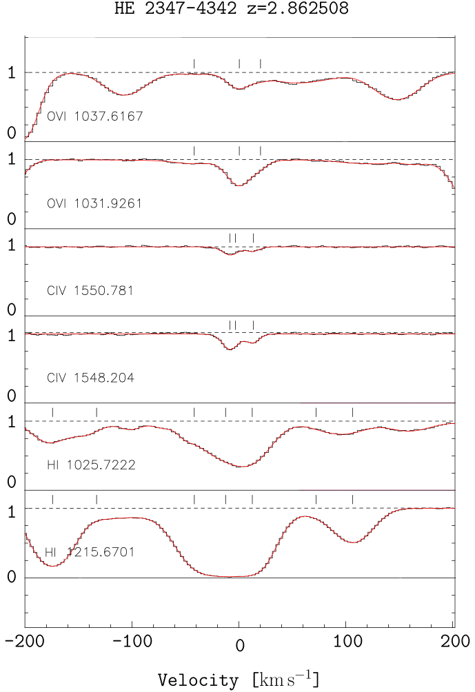
Figure C.1: HE 2347-4342 $z=2.862508$. This system is classified as category $2$.

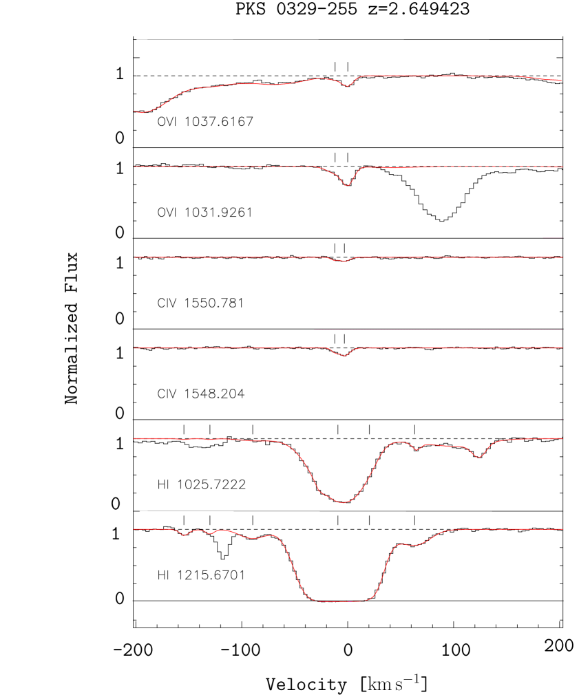
Figure C.2: PKS 0329-255 $z=2.649423$. This system is classified as category $2$.

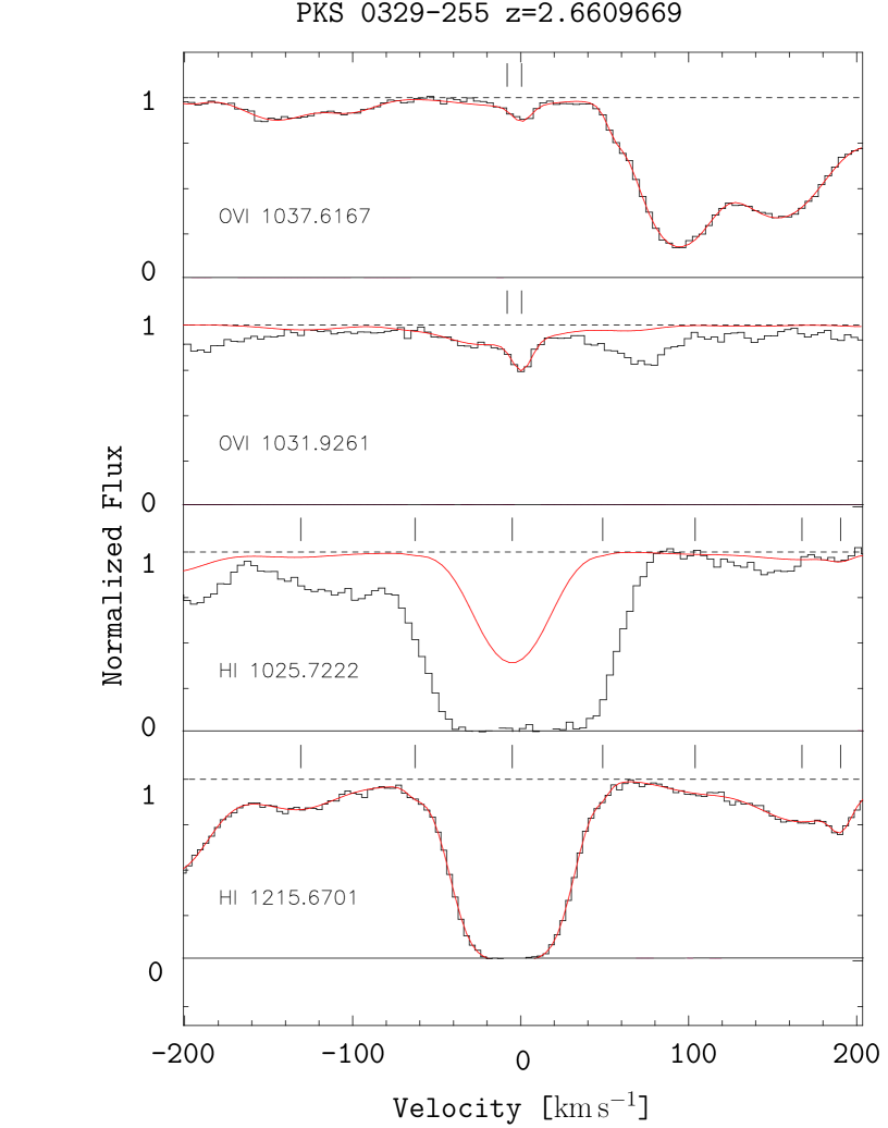
Figure C.3: PKS 0329-255 $z=2.6609669$. This system is classified as category $2$.

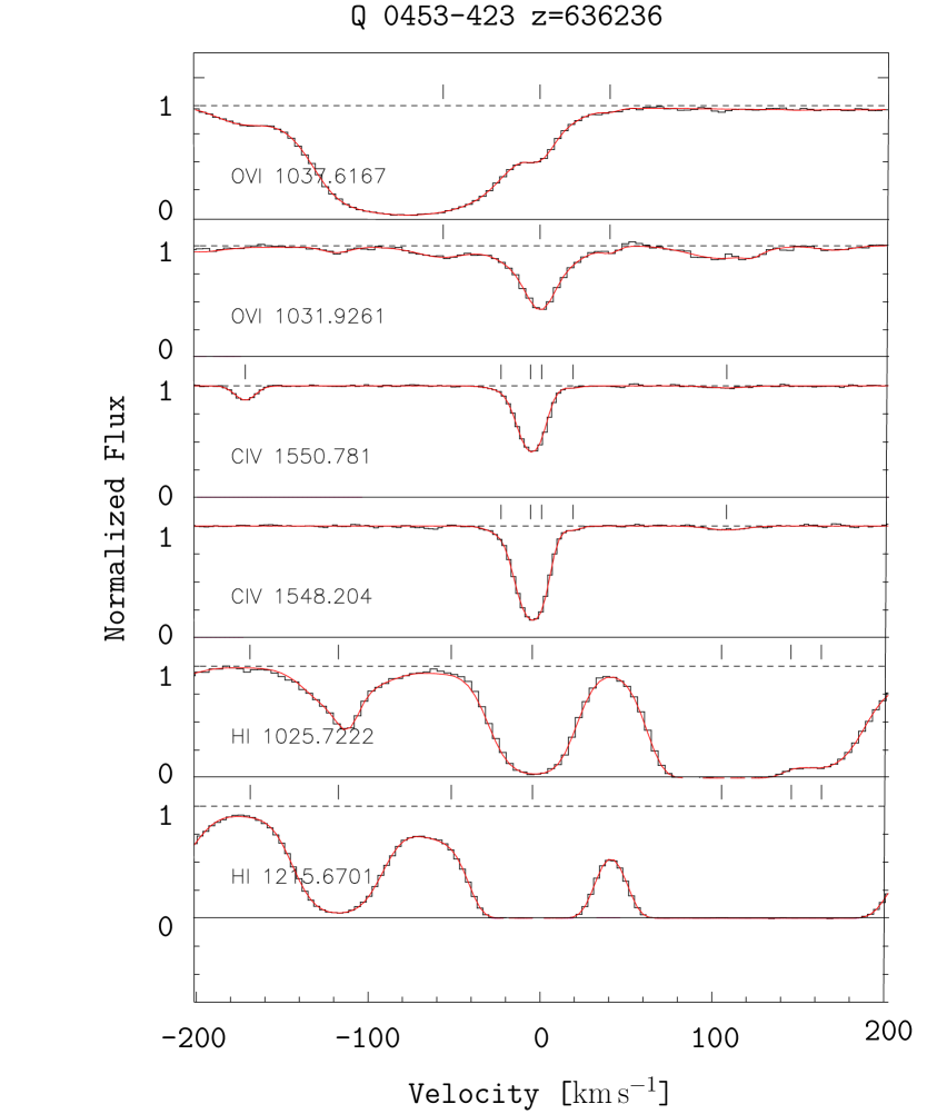
Figure C.4: Q 0453-423 $z=2.636236$. This system is classified as category $1$.

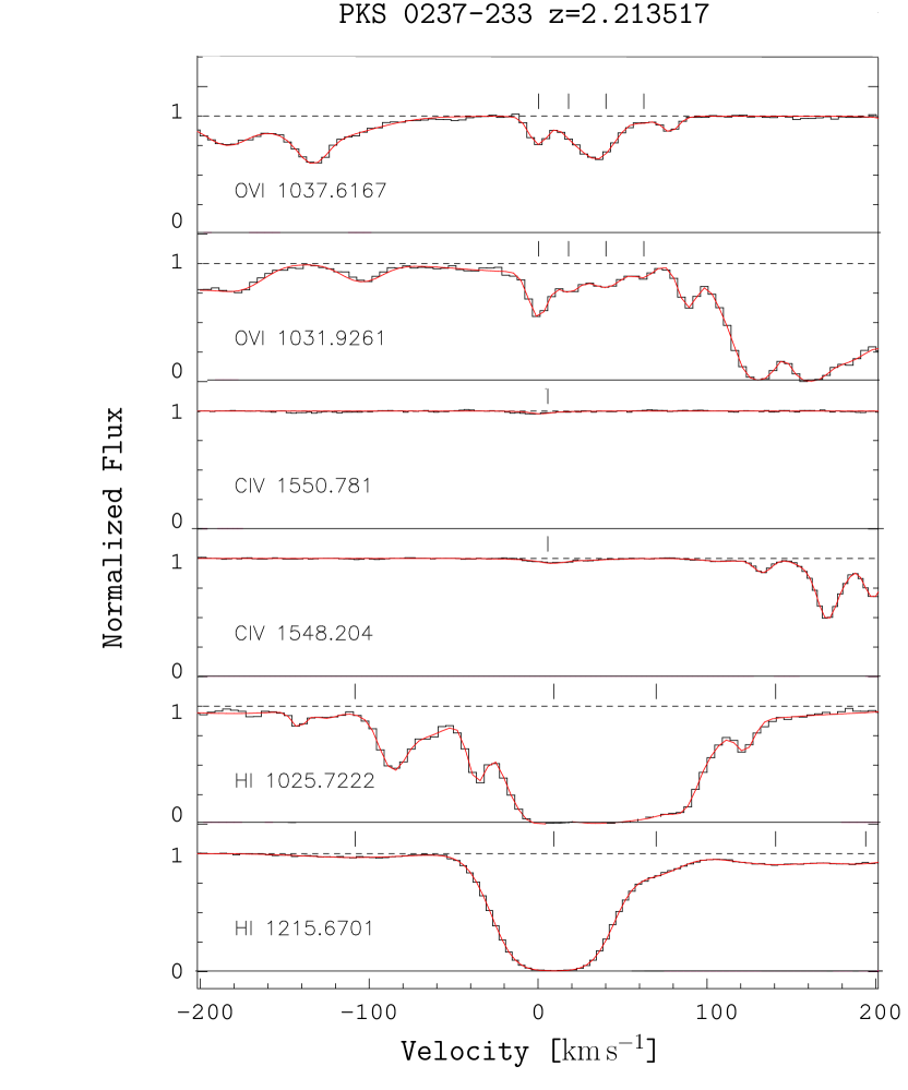
Figure C.5: PKS 0237-233 $z=2.213517$. This system is classified as category $1$.

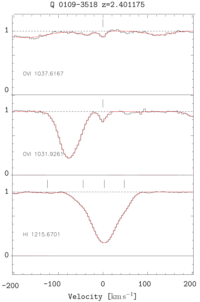
Figure C.6: Q 0109-3518 $z=2.401175$. This system is classified as category $1$.

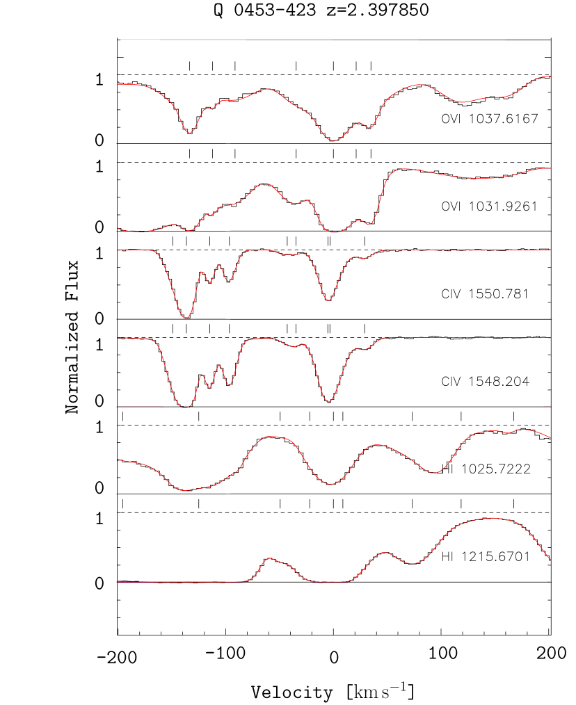
Figure C.7: Q 0453-423 $z=2.397850$. This system is classified as category $0$.

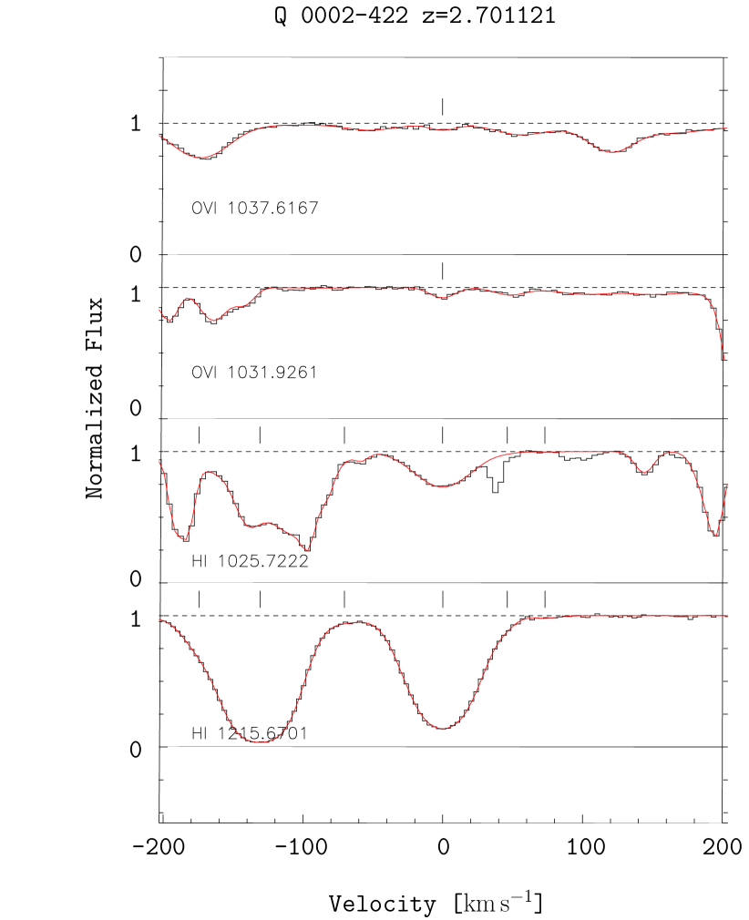
Figure C.8: Q 0002-422 $z=2.701121$. This system is classified as category $0$.

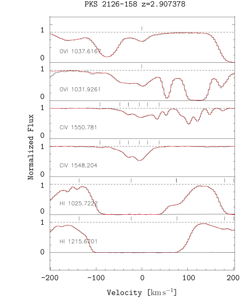
Figure C.9: PKS 2126-158 $z=2.907378$. This system is classified as category $0$.

C.2 Simulated (OWLS) absorption spectra - examples

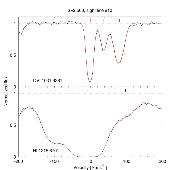
Figure C.10: Synthetic spectra of sightline No.10 at $z=2.50$. The (red and black) tick marks show the main components in the spectra. With red are shown the components with velocity alignment between O vi and H i ($\leq 10$ km $\rm s^{-1}$).

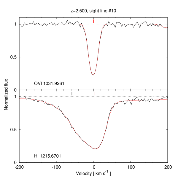
Figure C.11: Synthetic spectra of sightline No.10 at $z=2.50$. The tick marks are the same as in Fig. C.10.

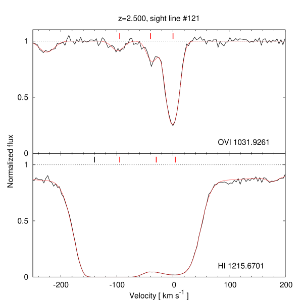
Figure C.12: Synthetic spectra of sightline No.121 at $z=2.50$. The tick marks are the same as in Fig. C.10.

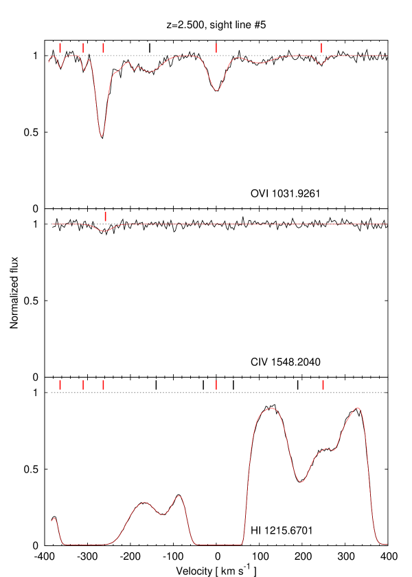
Figure C.13: Synthetic spectra of sightline No.5 at $z=2.50$. The black tick marks are the same as in Fig. C.10. The red show the components with velocity alignment between O vi ​​, (in some cases) C iv and H i ($\leq 10$ km $\rm s^{-1}$).

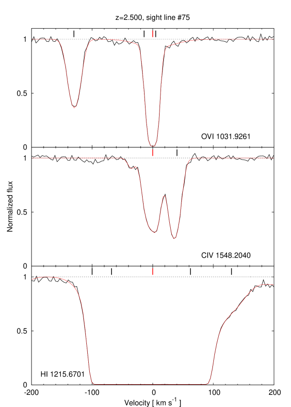
Figure C.14: Synthetic spectra of sightline No.75 at $z=2.50$. The tick marks are the same as in Fig. C.13.

Acknowledgments

First, I would like to thank my supervisor Prof. Philipp Richter for giving me the freedom and the support to accomplish this Thesis. I was glad to be a member of your group.

I am grateful to Thorsten Tepper-García for his guidance and care for my work. I appreciate it very much.

I would like to thank as well Cora Fechner, Martin Wendt and Andrea Brockhaus who were always there when I needed scientific or organizational advice.

Special thanks to Dominik Hildebrandt for the discussions about physics and life and for giving me great personal support.

I would like to thank also Prof. Matthias Steinmetz for his response to an e-mail from me when I was looking for an opportunity to continue my education in astrophysics in Germany.

Special thanks to Todor Veltchev for his full personal support throughout the years and for editing the language in this Thesis.

I am very thankful to my son for his understanding in moments when I had to work and had to leave him alone.

References

- Adams (1976) Adams, T. F. 1976, A&A, 50, 461
- Aguirre et al. (2008) Aguirre, A., Dow-Hygelund, C., Schaye, J., & Theuns, T. 2008, ApJ, 689, 851
- Anders & Grevesse (1989) Anders, E. & Grevesse, N. 1989, Geochim. Cosmochim. Acta, 53, 197
- Anderson et al. (1987) Anderson, S. F., Weymann, R. J., Foltz, C. B., & Chaffee, Jr., F. H. 1987, AJ, 94, 278
- Ben Bekhti et al. (2012) Ben Bekhti, N., Winkel, B., Richter, P., et al. 2012, A&A, 542, A110
- Bergeron et al. (2002) Bergeron, J., Aracil, B., Petitjean, P., & Pichon, C. 2002, A&A, 396, L11