Distillation as a Defense to Adversarial
Perturbations against Deep Neural Networks

Abstract

Deep learning algorithms have been shown to perform extremely well on many classical machine learning problems. However, recent studies have shown that deep learning, like other machine learning techniques, is vulnerable to adversarial samples: inputs crafted to force a deep neural network (DNN) to provide adversary-selected outputs. Such attacks can seriously undermine the security of the system supported by the DNN, sometimes with devastating consequences. For example, autonomous vehicles can be crashed, illicit or illegal content can bypass content filters, or biometric authentication systems can be manipulated to allow improper access. In this work, we introduce a defensive mechanism called defensive distillation to reduce the effectiveness of adversarial samples on DNNs. We analytically investigate the generalizability and robustness properties granted by the use of defensive distillation when training DNNs. We also empirically study the effectiveness of our defense mechanisms on two DNNs placed in adversarial settings. The study shows that defensive distillation can reduce effectiveness of sample creation from 95% to less than 0.5% on a studied DNN. Such dramatic gains can be explained by the fact that distillation leads gradients used in adversarial sample creation to be reduced by a factor of $10^{30}$. We also find that distillation increases the average minimum number of features that need to be modified to create adversarial samples by about 800% on one of the DNNs we tested.

I Introduction

Deep Learning (DL) has been demonstrated to perform exceptionally well on several categories of machine learning problems, notably input classification. These Deep Neural Networks (DNNs) efficiently learn highly accurate models from a large corpus of training samples, and thereafter classify unseen samples with great accuracy. As a result, DNNs are used in many settings [1, 2, 3], some of which are increasingly security-sensitive [4, 5, 6]. By using deep learning algorithms, designers of these systems make implicit security assumptions about deep neural networks. However, recent work in the machine learning and security communities have shown that adversaries can force many machine learning models, including DNNs, to produce adversary-selected outputs using carefully crafted inputs [7, 8, 9].

Specifically, adversaries can craft particular inputs, named adversarial samples, leading models to produce an output behavior of their choice, such as misclassification. Inputs are crafted by adding a carefully chosen adversarial perturbation to a legitimate sample. The resulting sample is not necessarily unnatural, i.e. outside of the training data manifold. Algorithms crafting adversarial samples are designed to minimize the perturbation, thus making adversarial samples hard to distinguish from legitimate samples. Attacks based on adversarial samples occur after training is complete and therefore do not require any tampering with the training procedure.

To illustrate how adversarial samples make a system based on DNNs vulnerable, consider the following input samples:

The left image is correctly classified by a trained DNN as a car. The right image was crafted by an adversarial sample algorithm (in [7]) from the correct left image. The altered image is incorrectly classified as a cat by the DNN. To see why such misclassification is dangerous, consider deep learning as it is commonly used in autonomous (driverless) cars [10]. Systems based on DNNs are used to recognize signs or other vehicles on the road [11]. If perturbing the input of such systems, by slightly altering the car’s body for instance, prevents DNNs from classifying it as a moving vehicule correctly, the car might not stop and eventually be involved in an accident, with potentially disastrous consequences. The threat is real where an adversary can profit from evading detection or having their input misclassified. Such attacks commonly occur today in non-DL classification systems [12, 13, 14, 15, 16].

Thus, adversarial samples must be taken into account when designing security sensitive systems incorporating DNNs. Unfortunately, there are very few effective countermeasures available today. Previous work considered the problem of constructing such defenses but solutions proposed are deficient in that they require making modifications to the DNN architecture or only partially prevent adversarial samples from being effective [9, 17] (see Section VII).

Distillation is a training procedure initially designed to train a DNN using knowledge transferred from a different DNN. The intuition was suggested in [18] while distillation itself was formally introduced in [19]. The motivation behind the knowledge transfer operated by distillation is to reduce the computational complexity of DNN architectures by transferring knowledge from larger architectures to smaller ones. This facilitates the deployment of deep learning in resource constrained devices (e.g. smartphones) which cannot rely on powerful GPUs to perform computations. We formulate a new variant of distillation to provide for defense training: instead of transferring knowledge between different architectures, we propose to use the knowledge extracted from a DNN to improve its own resilience to adversarial samples.

In this paper, we explore analytically and empirically the use of distillation as a defensive mechanism against adversarial samples. We use the knowledge extracted during distillation to reduce the amplitude of network gradients exploited by adversaries to craft adversarial samples. If adversarial gradients are high, crafting adversarial samples becomes easier because small perturbations will induce high DNN output variations. To defend against such perturbations, one must therefore reduce variations around the input, and consequently the amplitude of adversarial gradients. In other words, we use defensive distillation to smooth the model learned by a DNN architecture during training by helping the model generalize better to samples outside of its training dataset.

At test time, models trained with defensive distillation are less sensitive to adversarial samples, and are therefore more suitable for deployment in security sensitive settings. We make the following contributions in this paper:

• We articulate the requirements for the design of adversarial sample DNN defenses. These guidelines highlight the inherent tension between defensive robustness, output accuracy, and performance of DNNs.

• We introduce defensive distillation, a procedure to train DNN-based classifier models that are more robust to perturbations. Distillation extracts additional knowledge about training points as class probability vectors produced by a DNN, which is fed back into the training regimen. This departs substantially from the past uses of distillation which aimed to reduce the DNN architectures to improve computational performance, but rather feeds the gained knowledge back into the original models.

• We analytically investigate defensive distillation as a security countermeasure. We show that distillation generates smoother classifier models by reducing their sensitivity to input perturbations. These smoother DNN classifiers are found to be more resilient to adversarial samples and have improved class generalizability properties.

• We show empirically that defensive distillation reduces the success rate of adversarial sample crafting from $95.89\%$ to $0.45\%$ against a first DNN trained on the MNIST dataset [20], and from $87.89\%$ to $5.11\%$ against a second DNN trained on the CIFAR10 [21] dataset.

• A further empirical exploration of the distillation parameter space shows that a correct parameterization can reduce the sensitivity of a DNN to input perturbations by a factor of $10^{30}$. Successively, this increases the average minimum number of input features to be perturbed to achieve adversarial targets by $790\%$ for a first DNN, and by $556\%$ for a second DNN.

II Adversarial Deep Learning

Deep learning is an established technique in machine learning. In this section, we provide some rudiments of deep neural networks (DNNs) necessary to understand the subtleties of their use in adversarial settings. We then formally describe two attack methods in the context of a framework that we construct to (i) develop an understanding of DNN vulnerabilities exploited by these attacks and (ii) compare the strengths and weaknesses of both attacks in various adversarial settings. Finally, we provide an overview of a DNN training procedure, which our defense mechanism builds on, named distillation.

II-A Deep Neural Networks in Adversarial Settings

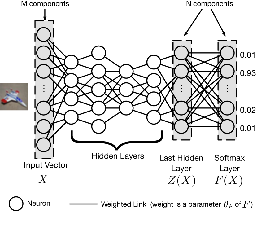
Figure 1: Overview of a DNN architecture: This architecture, suitable for classification tasks thanks to its softmax output layer, is used throughout the paper along with its notations.

Training and deploying DNN architectures - Deep neural networks compose many parametric functions to build increasingly complex representations of a high dimensional input expressed in terms of previous simpler representations [22]. Practically speaking, a DNN is made of several successive layers of neurons building up to an output layer. These layers can be seen as successive representations of the input data [23], a multidimensional vector $X$, each of them corresponding to one of the parametric functions mentioned above. Neurons constituting layers are modeled as elementary computing units applying an activation function to their input. Layers are connected using links weighted by a set of vectors, also referred to as network parameters $\theta_{F}$. Figure 1 illustrates such an architecture along with notations used in this paper.

The numerical values of weight vectors in $\theta_{F}$ are evaluated during the network’s training phase. During that phase, the DNN architecture is given a large set of known input-output pairs $(X,Y)\in(\cal{X},\cal{Y})$. It uses a series of successive forward and backward passes through the DNN layers to compute prediction errors made by the output layer of the DNN, and corresponding gradients with respect to weight parameters [24]. The weights are then updated, using the previously described gradients, in order to improve the prediction and eventually the overall accuracy of the network. This training process is referred to as backpropagation and is governed by hyper-parameters essential to the convergence of model weight [25]. The most important hyper-parameter is the learning rate that controls the speed at which weights are updated with gradients.

Once the network is trained, the architecture together with its parameter values $\theta_{F}$ can be considered as a classification function $F$ and the test phase begins: the network is used on unseen inputs $X$ to predict outputs $F(X)$. Weights learned during training hold knowledge that the DNN applies to these new and unseen inputs. Depending on the type of output expected from the network, we either refer to supervised learning when the network must learn some association between inputs and outputs (e.g., classification [1, 4, 11, 26]) or unsupervised learning when the network is trained with unlabeled inputs (e.g., dimensionality reduction, feature engineering, or network pre-training [21, 27, 28]). In this paper, we only consider supervised learning, and more specifically the task of classification. The goal of the training phase is to enable the neural network to extrapolate from the training data it observed during training so as to correctly predict outputs on new and unseen samples at test time.

Adversarial Deep Learning - It has been shown in previous work that when DNNs are deployed in adversarial settings, one must take into account certain vulnerabilities [7, 8, 9]. Namely, adversarial samples are artifacts of a threat vector against DNNs that can be exploited by adversaries at test time, after network training is completed. Crafted by adding carefully selected perturbations $\delta X$ to legitimate inputs $X$, their key property is to provoke a specific behavior from the DNN, as initially chosen by the adversary. For instance, adversaries can alter samples to have them misclassified by a DNN, as is the case of adversarial samples crafted in experiments presented in section V, some of which are illustrated in Figure 2. Note that the noise introduced by perturbation $\delta X$ added to craft the adversarial sample must be small enough to allow a human to still correctly process the sample.

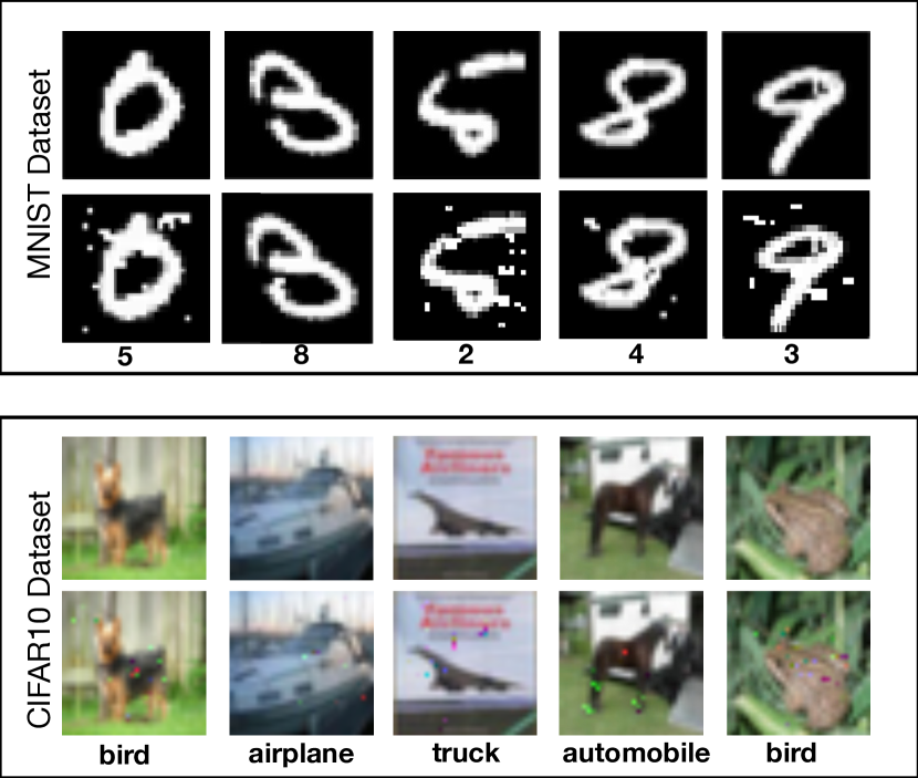
Figure 2: Set of legitimate and adversarial samples for two datasets: For each dataset, a set of legitimate samples, which are correctly classified by DNNs, can be found on the top row while a corresponding set of adversarial samples (crafted using [7]), misclassifed by DNNs, are on the bottom row.

Attacker’s end goals can be quite diverse, as pointed out in previous work formalizing the space of adversaries against deep learning [7]. For classifiers, they range from simple confidence reduction (where the aim is to reduce a DNN’s confidence on a prediction, thus introducing class ambiguity), to source-target misclassification (where the goal is to be able to take a sample from any source class and alter it so as to have the DNN classify it in any chosen target class distinct from the source class). This paper considers the source-target misclassification, also known as the chosen target attack, in the following sections. Potential examples of adversarial samples in realistic contexts could include slightly altering malware executables in order to evade detection systems built using DNNs, adding perturbations to handwritten digits on a check resulting in a DNN wrongly recognizing the digits (for instance, forcing the DNN to read a larger amount than written on the check), or altering a pattern of illegal financial operations to prevent it from being picked up by fraud detections systems using DNNs. Similar attacks occur today on non-DNN classification systems [12, 13, 14, 15] and are likely to be ported by adversaries to DNN classifiers.

As explained later in the attack framework described in this section, methods for crafting adversarial samples theoretically require a strong knowledge of the DNN architecture. However in practice, even attackers with limited capabilities can perform attacks by approximating their target DNN model $F$ and crafting adversarial samples on this approximated model. Indeed, previous work reported that adversarial samples against DNNs are transferable from one model to another [8]. Skilled adversaries can thus train their own DNNs to produce adversarial samples evading victim DNNs. Therefore throughout this paper, we consider an attacker with the capability of accessing a trained DNN used for classification, since the transferability of adversarial samples makes this assumption acceptable. Such a capability can indeed take various forms including for instance a direct access to the network architecture implementation and parameters, or access to the network as an oracle requiring the adversary to approximatively replicate the model. Note that we do not consider attacks at training time in this paper and leave such considerations to future work.

II-B Adversarial Sample Crafting

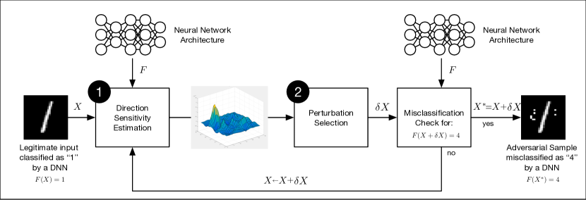
Figure 3: Adversarial crafting framework: Existing algorithms for adversarial sample crafting [7, 9] are a succession of two steps: (1) direction sensitivity estimation and (2) perturbation selection. Step (1) evaluates the sensitivity of model $F$ at the input point corresponding to sample $X$. Step (2) uses this knowledge to select a perturbation affecting sample $X$’s classification. If the resulting sample $X+\delta X$ is misclassified by model $F$ in the adversarial target class (here 4) instead of the original class (here 1), an adversarial sample $X^{*}$ has been found. If not, the steps can be repeated on updated input $X\leftarrow X+\delta X$.

We now describe precisely how adversarial sample are crafted by adversaries. The general framework we introduce builds on previous attack approaches and is split in two folds: direction sensitivity estimation and perturbation selection. Attacks holding in this framework correspond to adversaries with diverse goals, including the goal of misclassifying samples from a specific source class into a distinct target class. This is one of the strongest adversarial goals for attacks targeting classifiers at test time and several other goals can be achieved if the adversary has the capability of achieving this goal. More specifically, consider a sample $X$ and a trained DNN resulting in a classifier model $F$. The goal of the adversary is to produce an adversarial sample $X^{*}=X+\delta X$ by adding a perturbation $\delta X$ to sample $X$, such that $F(X^{*})=Y^{*}$ where $Y^{*}\neq F(X)$ is the adversarial target output taking the form of an indicator vector for the target class [7].

As several approaches at adversarial sample crafting have been proposed in previous work, we now construct a framework that encompasses these approaches, for future work to build on. This allows us to compare the strengths and weaknesses of each method. The resulting crafting framework is illustrated in Figure 3. Broadly speaking, an adversary starts by considering a legitimate sample $X$. We assume that the adversary has the capability of accessing parameters $\theta_{F}$ of his targeted model $F$ or of replicating a similar DNN architecture (since adversarial samples are transferable between DNNs) and therefore has access to its parameter values. The adversarial sample crafting is then a two-step process:

1. Direction Sensitivity Estimation: evaluate the sensitivity of class change to each input feature

2. Perturbation Selection: use the sensitivity information to select a perturbation $\delta X$ among the input dimensions

In other terms, step (1) identifies directions in the data manifold around sample $X$ in which the model $F$ learned by the DNN is most sensitive and will likely result in a class change, while step (2) exploits this knowledge to find an effective adversarial perturbation. Both steps are repeated if necessary, by replacing $X$ with $X+\delta X$ before starting each new iteration, until the sample satisfies the adversarial goal: it is classified by deep neural networks in the target class specified by the adversary using a class indicator vector $Y^{*}$. Note that, as mentioned previously, it is important for the total perturbation used to craft an adversarial sample from a legitimate sample to be minimized, at least approximatively. This is essential for adversarial samples to remain undetected, notably by humans. Crafting adversarial samples using large perturbations would be trivial. Therefore, if one defines a norm $\|\cdot\|$ appropriate to describe differences between points in the input domain of DNN model $F$, adversarial samples can be formalized as a solution to the following optimization problem:

$$\arg\min_{\delta X}\|\delta X\|\mbox{ s.t. }F(X+\delta X)=Y^{*}$$ (1)

Most DNN models $F$ will make this problem non-linear and non-convex, making a closed-solution hard to find in most cases. We now describe in details our attack framework approximating the solution to this optimization problem, using previous work to illustrate each of the two steps.

Direction Sensitivity Estimation - This step considers sample $X$, a $M$-dimensional input. The goal here is to find the dimensions of $X$ that will produce the expected adversarial behavior with the smallest perturbation. To achieve this, the adversary must evaluate the sensitivity of the trained DNN model $F$ to changes made to input components of $X$. Building such a knowledge of the network sensitivity can be done in several ways. Goodfellow et al. [9] introduced the fast sign gradient method that computes the gradient of the cost function with respect to the input of the neural network. Finding sensitivities is then achieved by applying the cost function to inputs labeled using adversarial target labels. Papernot et al. [7] took a different approach and introduced the forward derivative, which is the Jacobian of $F$, thus directly providing gradients of the output components with respect to each input component. Both approaches define the sensitivity of the network for the given input $X$ in each of its dimensions [7, 9]. Miyato et al. [29] introduced another sensitivity estimation measure, named the Local Distribution Smoothness, based on the Kullback-Leibler divergence, a measure of the difference between two probability distributions. To compute it, they use an approximation of the network’s Hessian matrix. They however do not present any results on adversarial sample crafting, but instead focus on using the local distribution smoothness as a training regularizer improving the classification accuracy.

Perturbation Selection - The adversary must now use this knowledge about the network sensitivity to input variations to evaluate which dimensions are most likely to produce the target misclassification with a minimum total perturbation vector $\delta X$. Each of the two techniques takes a different approach again here, depending on the distance metric used to evaluate what a minimum perturbation is. Goodfellow et al. [9] choose to perturb all input dimensions by a small quantity in the direction of the sign of the gradient they computed. This effectively minimizes the Euclidian distance between the original and the adversarial samples. Papernot et al. [7] take a different approach and follow a more complex process involving saliency maps to only select a limited number of input dimensions to perturb. Saliency maps assign values to combinations of input dimensions indicating whether they will contribute to the adversarial goal or not if perturbed. This effectively diminishes the number of input features perturbed to craft samples. The amplitude of the perturbation added to each input dimensions is a fixed parameter in both approaches. Depending on the input nature (images, malware, …), one method or the other is more suitable to guarantee the existence of adversarial samples crafted using an acceptable perturbation $\delta X$. An acceptable perturbation is defined in terms of a distance metric over the input dimensions (e.g., a $L1,L2$ norm). Depending on the problem nature, different metrics apply and different perturbation shapes are acceptable or not.

II-C About Neural Network Distillation

We describe here the approach to distillation introduced by Hinton et al. [19]. Distillation is motivated by the end goal of reducing the size of DNN architectures or ensembles of DNN architectures, so as to reduce their computing ressource needs, and in turn allow deployment on resource constrained devices like smartphones. The general intuition behind the technique is to extract class probability vectors produced by a first DNN or an ensemble of DNNs to train a second DNN of reduced dimensionality without loss of accuracy.

This intuition is based on the fact that knowledge acquired by DNNs during training is not only encoded in weight parameters learned by the DNN but is also encoded in the probability vectors produced by the network. Therefore, distillation extracts class knowledge from these probability vectors to transfer it into a different DNN architecture during training. To perform this transfer, distillation labels inputs in the training dataset of the second DNN using their classification predictions according to the first DNN. The benefit of using class probabilities instead of hard labels is intuitive as probabilities encode additional information about each class, in addition to simply providing a sample’s correct class. Relative information about classes can be deduced from this extra entropy.

To perform distillation, a large network whose output layer is a softmax is first trained on the original dataset as would usually be done. An example of such a network is depicted in Figure 1. A softmax layer is merely a layer that considers a vector $Z(X)$ of outputs produced by the last hidden layer of a DNN, which are named logits, and normalizes them into a probability vector $F(X)$, the ouput of the DNN, assigning a probability to each class of the dataset for input $X$. Within the softmax layer, a given neuron corresponding to a class indexed by $i\in 0..N-1$ (where $N$ is the number of classes) computes component $i$ of the following output vector $F(X)$:

$$F(X)=\left[\frac{e^{z_{i}(X)/T}}{\sum_{l=0}^{N-1}e^{z_{l}(X)/T}}\right]_{i\in 0..N-1}$$ (2)

where $Z(X)=z_{0}(X),...,z_{N-1}(X)$ are the $N$ logits corresponding to the hidden layer outputs for each of the $N$ classes in the dataset, and $T$ is a parameter named temperature and shared across the softmax layer. Temperature plays a central role in underlying phenomena of distillation as we show later in this section. In the context of distillation, we refer to this temperature as the distillation temperature. The only constraint put on the training of this first DNN is that a high temperature, larger than 1, should be used in the softmax layer.

The high temperature forces the DNN to produce probability vectors with relatively large values for each class. Indeed, at high temperatures, logits in vector $Z(X)$ become negligible compared to temperature $T$. Therefore, all components of probability vector $F(X)$ expressed in Equation 2 converge to $1/N$ as $T\rightarrow\infty$. The higher the temperature of a softmax is, the more ambiguous its probability distribution will be (i.e. all probabilities of the output $F(X)$ are close to $1/N$), whereas the smaller the temperature of a softmax is, the more discrete its probability distribution will be (i.e. only one probability in output $F(X)$ is close to $1$ and the remainder are close to $0$).

The probability vectors produced by the first DNN are then used to label the dataset. These new labels are called soft labels as opposed to hard class labels. A second network with less units is then trained using this newly labelled dataset. Alternatively, the second network can also be trained using a combination of the hard class labels and the probability vector labels. This allows the network to benefit from both labels to converge towards an optimal solution. Again, the second network is trained at a high softmax temperature identical to the one used in the first network. This second model, although of smaller size, achieves comparable accuracy than the original model but is less computationally expensive. The temperature is set back to 1 at test time so as to produce more discrete probability vectors during classification.

III Defending DNNs using Distillation

Armed with background on DNNs in adversarial settings, we now introduce a defensive mechanism to reduce vulnerabilities exposing DNNs to adversarial samples. We note that most previous work on combating adversarial samples proposed regularizations or dataset augmentations. We instead take a radically different approach and use distillation, a training technique described in the previous section, to improve the robustness of DNNs. We describe how we adapt distillation into defensive distillation to address the problem of DNN vulnerability to adversarial perturbations. We provide a justification of the approach using elements from learning theory.

III-A Defending against Adversarial Perturbations

To formalize our discussion of defenses against adversarial samples, we now propose a metric to evaluate the resilience of DNNs to adversarial noise. To build an intuition for this metric, namely the robustness of a network, we briefly comment on the underlying vulnerabilities exploited by the attack framework presented above. We then formulate requirements for defenses capable of enhancing classification robustness.

In the framework discussed previously, we underlined the fact that attacks based on adversarial samples were primarily exploiting gradients computed to estimate the sensitivity of networks to its input dimensions. To simplify our discussion, we refer to these gradients as adversarial gradients in the remainder of this document. If adversarial gradients are high, crafting adversarial samples becomes easier because small perturbations will induce high network output variations. To defend against such perturbations, one must therefore reduce these variations around the input, and consequently the amplitude of adversarial gradients. In other words, we must smooth the model learned during training by helping the network generalize better to samples outside of its training dataset. Note that adversarial samples are not necessarily found in “nature”, because adversarial samples are specifically crafted to break the classification learned by the network. Therefore, they are not necessarily extracted from the input distribution that the DNN architecture tries to model during training.

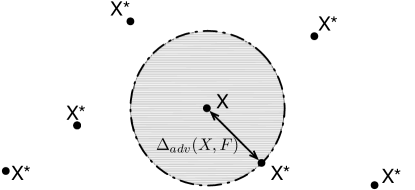
Figure 4: Visualizing the hardness metric: This 2D representation illustrates the hardness metric as the radius of the disc centered at the original sample $X$ and going through the closest adversarial sample $X^{*}$ among all the possible adversarial samples crafted from sample $X$. Inside the disc, the class output by the classifier is constant. However, outside the disc, all samples $X^{*}$ are classified differently than $X$.

DNN Robustness - We informally defined the notion of robustness of a DNN to adversarial perturbations as its capability to resist perturbations. In other words, a robust DNN should (i) display good accuracy inside and outside of its training dataset as well as (ii) model a smooth classifier function $F$ which would intuitively classify inputs relatively consistently in the neighborhood of a given sample. The notion of neighborhood can be defined by a norm appropriate for the input domain. Previous work has formalized a close definition of robustness in the context of other machine learning techniques [30]. The intuition behind this metric is that robustness is achieved by ensuring that the classification output by a DNN remains somewhat constant in a closed neighborhood around any given sample extracted from the classifier’s input distribution. This idea is illustrated in Figure 4. The larger this neighborhood is for all inputs within the natural distribution of samples, the more robust is the DNN. Not all inputs are considered, otherwise the ideal robust classifier would be a constant function, which has the merit of being very robust to adversarial perturbations but is not a very interesting classifier. We extend the definition of robustness introduced in [30] to the adversarial behavior of source-target class pair misclassification within the context of classifiers built using DNNs. The robustness of a trained DNN model $F$ is:

$$\rho_{adv}(F)=E_{\mu}[\Delta_{adv}(X,F)]$$ (3)

where inputs $X$ are drawn from distribution $\mu$ that DNN architecture is attempting to model with $F$, and $\Delta_{adv}(X,F)$ is defined to be the minimum perturbation required to misclassify sample $x$ in each of the other classes:

$$\Delta_{adv}(X,F)=\arg\min_{\delta X}\{\|\delta X\|:F(X+\delta X)\neq F(X)\}$$ (4)

where $\|\cdot\|$ is a norm and must be specified accordingly to the context. The higher the average minimum perturbation required to misclassify a sample from the data manifold is, the more robust the DNN is to adversarial samples.

Defense Requirements - Pulling from this formalization of DNN robustness. we now outline design requirements for defenses against adversarial perturbations:

• Low impact on the architecture: techniques introducing limited, modifications to the architecture are preferred in our approach because introducing new architectures not studied in the literature requires analysis of their behaviors. Designing new architectures and benchmarking them against our approach is left as future work.

• Maintain accuracy: defenses against adversarial samples should not decrease the DNN’s classification accuracy. This discards solutions based on weight decay, through $L1,L2$ regularization, as they will cause underfitting.

• Maintain speed of network: the solutions should not significantly impact the running time of the classifier at test time. Indeed, running time at test time matters for the usability of DNNs, whereas an impact on training time is somewhat more acceptable because it can be viewed as a fixed cost. Impact on training should nevertheless remain limited to ensure DNNs can still take advantage of large training datasets to achieve good accuracies. For instance, solutions based on Jacobian regularization, like double backpropagation [31], or using radial based activation functions [9] degrade DNN training performance.

• Defenses should work for adversarial samples relatively close to points in the training dataset [9, 7]. Indeed, samples that are very far away from the training dataset, like those produced in [32], are irrelevant to security because they can easily be detected, at least by humans. However, limiting sensitivity to infinitesimal perturbation (e.g., using double backpropagation [31]) only provides constraints very near training examples, so it does not solve the adversarial perturbation problem. It is also very hard or expensive to make derivatives smaller to limit sensitivity to infinitesimal perturbations.

We show in our approach description below that our defense technique does not require any modification of the neural network architecture and that it has a low overhead on training and no overhead on test time. In the evaluation conducted in section V, we also show that our defense technique fits the remaining defense requirements by evaluating the accuracy of DNNs with and without our defense deployed, and studying the generalization capabilities of networks to show how the defense impacted adversarial samples.

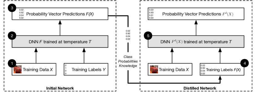
Figure 5: An overview of our defense mechanism based on a transfer of knowledge contained in probability vectors through distillation: We first train an initial network $F$ on data $X$ with a softmax temperature of $T$. We then use the probability vector $F(X)$, which includes additional knowledge about classes compared to a class label, predicted by network $F$ to train a distilled network $F^{d}$ at temperature $T$ on the same data $X$.

III-B Distillation as a Defense

We now introduce defensive distillation, which is the technique we propose as a defense for DNNs used in adversarial settings, when adversarial samples cannot be permitted. Defensive distillation is adapted from the distillation procedure, presented in section II, to suit our goal of improving DNN classification resilience in the face of adversarial perturbations.

Our intuition is that knowledge extracted by distillation, in the form of probability vectors, and transferred in smaller networks to maintain accuracies comparable with those of larger networks can also be beneficial to improving generalization capabilities of DNNs outside of their training dataset and therefore enhances their resilience to perturbations. Note that throughout the remainder of this paper, we assume that considered DNNs are used for classification tasks and designed with a softmax layer as their output layer.

The main difference between defensive distillation and the original distillation proposed by Hinton et al. [19] is that we keep the same network architecture to train both the original network as well as the distilled network. This difference is justified by our end which is resilience instead of compression. The resulting defensive distillation training procedure is illustrated in Figure 5 and outlined as follows:

1. The input of the defensive distillation training algorithm is a set $\cal X$ of samples with their class labels. Specifically, let $X\in{\cal X}$ be a sample, we use $Y(X)$ to denote its discrete label, also referred to as hard label. $Y(X)$ is an indicator vector such that the only non-zero element corresponds to the correct class’ index (e.g. $(0,0,1,0,\dots,0)$ indicates that the sample is in the class with index $2$).

2. Given this training set $\{(X,Y(X)):X\in\cal{X}\}$, we train a deep neural network $F$ with a softmax output layer at temperature $T$. As we discussed before, $F(X)$ is a probability vector over the class of all possible labels. More precisely, if the model $F$ has parameters $\theta_{F}$, then its output on $X$ is a probability distribution $F(X)=p(\cdot|X,\theta_{F})$, where for any label $Y$ in the label class, $p(Y|X,\theta_{F})$ gives a probability that the label is $Y$. To simplify our notation later, we use $F_{i}(X)$ to denote the probability of input $X$ to be in class $i\in 0..N-1$ according to model $F$ with parameters $\theta_{F}$.

3. We form a new training set, by consider samples of the form $(X,F(X))$ for $X\in{\cal X}$. That is, instead of using hard class label $Y(X)$ for $X$, we use the soft-target $F(X)$ encoding $F$’s belief probabilities over the label class.

4. Using the new training set $\{(X,F(X)):X\in{\cal X}\}$ we then train another DNN model $F^{d}$, with the same neural network architecture as $F$, and the temperature of the softmax layer remains $T$. This new model is denoted as $F^{d}$ and referred to as the distilled model.

Again, the benefit of using soft-targets $F(X)$ as training labels lies in the additional knowledge found in probability vectors compared to hard class labels. This additional entropy encodes the relative differences between classes. For instance, in the context of digit recognition developed later in section V, given an image $X$ of some handwritten digit, model $F$ may evaluate the probability of class $7$ to $F_{7}(X)=0.6$ and the probability of label $1$ to $F_{1}(X)=0.4$, which then indicates some structural similarity between $7$s and $1$s.

Training a network with this explicit relative information about classes prevents models from fitting too tightly to the data, and contributes to a better generalization around training points. Note that the knowledge extraction performed by distillation is controlled by a parameter: the softmax temperature $T$. As described in section II, high temperatures force DNNs to produce probabilities vectors with large values for each class. In sections IV and V, we make this intuition more precise with a theoretical analysis and an empirical evaluation.

IV Analysis of Defensive Distillation

We now explore analytically the impact of defensive distillation on DNN training and resilience to adversarial samples. As stated above, our intuition is that probability vectors produced by model $F$ encode supplementary entropy about classes that is beneficial during the training of distilled model $F^{d}$. Before proceeding further, note that our purpose in this section is not to provide a definitive argument about using defensive distillation to combat adversarial perturbations, but rather we view it as an initial step towards drawing a connection between distillation, learning theory, and DNN robustness for future work to build upon. This analysis of distillation is split in three folds studying (1) network training, (2) model sensitivity, and (3) the generalization capabilities of a DNN.

Note that with training, we are looking to converge towards a function $F^{*}$ resilient to adversarial noise and capable of generalizing better. The existence of function $F^{*}$ is guaranteed by the universality theorem for neural networks [33], which states that with enough neurons and enough training points, one can approximate any continuous function with arbitrary precision. In other words, according to this theorem, we know that there exists a neural network architecture that converges to $F^{*}$ if it is trained on a sufficient number of samples. With this result in mind, a natural hypothesis is that distillation helps convergence of DNN models towards the optimal function $F^{*}$ instead of a different local optimum during training.

IV-A Impact of Distillation on Network Training

To precisely understand the effect of defensive distillation on adversarial crafting, we need to analyze more in depth the training process. Throughout this analysis, we frequently refer to the training steps for defensive distillation, as described in Section III. Let us start by considering the training procedure of the first model $F$, which corresponds to step (2) of defensive distillation. Given a batch of samples $\{(X,Y(X))\ |\ X\in{\cal X}\}$ labeled with their correct classes, training algorithms typically aim to solve the following optimization problem:

$$\arg\min_{\theta_{F}}-\frac{1}{|{\cal X}|}\sum_{X\in{\cal X}}\sum_{i\in 0..N}Y_{i}(X)\log{F_{i}(X)}.$$ (5)

where $\theta_{F}$ is the set of parameters of model $F$ and $Y_{i}$ is the $i^{th}$ component of $Y$. That is, for each sample $(X,Y(X))$ and hypothesis, i.e. a model $F$ with parameters $\theta_{F}$, we consider the log-likelihood $\ell(F,X,Y(X))=-Y(X)\cdot\log{F(X)}$ of $F$ on $(X,Y(X))$ and average it over the entire training set $\cal{X}$. Very roughly speaking, the goal of this optimization is to adjust the weights of the model so as to push each $F(X)$ towards $Y(X)$. However, readers will notice that since $Y(X)$ is an indicator vector of input $X$’s class, Equation 5 can be simplified to:

$$\arg\min_{\theta_{F}}-\frac{1}{|{\cal X}|}\sum_{X\in{\cal X}}\log{F_{t(X)}(X)}.$$ (6)

where $t(X)$ is the only element in indicator vector $Y(X)$ that is equal to $1$, in other words the index of the sample’s class. This means that when performing updates to $\theta_{F}$, the training algorithm will constrain any output neuron different from the one corresponding to probability $F_{t(X)}(X)$ to give a $0$ output. However, this forces the DNN to make overly confident predictions in the sample class. We argue that this is a fundamental lack of precision during training as most of the architecture remains unconstrained as weights are updated.

Let us move on to explain how defensive distillation solves this issue, and how the distilled model $F^{d}$ is trained. As mentioned before, while the original training dataset is $\{(X,Y(X)):X\in{\cal X}\}$, the distilled model $F^{d}$ is trained using the same set of samples but labeled with soft-targets $\{(X,F(X)):X\in{\cal X}\}$ instead. This set is constructed at step (3) of defensive distillation. In other words, the label of $X$ is no longer the indicator vector $Y(X)$ corresponding to the hard class label of $X$, but rather the soft label of input $X$: a probability vector $F(X)$. Therefore, $F^{d}$ is trained, at step (4), by solving the following optimization problem:

$$\arg\min_{\theta_{F}}-\frac{1}{|{\cal X}|}\sum_{X\in{\cal X}}\sum_{i\in 0..N}F_{i}(X)\log{F_{i}^{d}(X)}$$ (7)

Note that the key difference here is that because we are using soft labels $F(X)$, it is not trivial anymore that most components of the double sum are null. Instead, using probabilities $F_{j}(X)$ ensures that the training algorithm will constrain all output neurons $F_{j}^{d}(X)$ proportionally to their likelihood when updating parameters $\theta_{F}$. We argue that this contributes to improving the generalizability of classifier model $F$ outside of its training dataset, by avoiding situations where the model is forced to make an overly confident prediction in one class when a sample includes characteristics of two or more classes (for instance, when classifying digits, an instance of a 8 include shapes also characteristic of a digit 3).

Note that model $F^{d}$ should theoretically eventually converge towards $F$. Indeed, locally at each point $(X,F(X))$, the optimal solution is for model $F^{d}$ to be such that $F^{d}(X)=F(X)$. To see this, we observe that training aims to minimize the cross entropy between $F^{d}(X)$ and $F(X)$, which is equal to:

$${\rm H}\left(F^{d}(X),F(X)\right)={\rm H}(F(X))+{\rm KL}\big{(}F(X)\ \|\ F^{d}(X)\big{)}$$ (8)

where ${\rm H}(F(X))$ is the Shannon entropy of $F(X)$) and ${\rm KL}$ denotes the Kullback-Leibler divergence. Note that this quantity is minimized when the KL divergence is equal to $0$, which is only true when $F^{d}(X)=F(X)$. Therefore, an ideal training procedure would result in model $F^{d}$ converging to the first model $F$. However, empirically this is not the case because training algorithms approximate the solution of the training optimization problem, which is often non-linear and non-convex. Furthermore, training algorithms only have access to a finite number of samples. Thus, we do observe empirically a better behavior in adversarial settings from model $F^{d}$ than model $F$. We confirm this result in Section V.

IV-B Impact of Distillation on Model Sensitivity

Having studied the impact of defensive distillation on optimization problems solved during DNN training, we now further investigate why adversarial perturbations are harder to craft on DNNs trained with defensive distillation at high temperature. The goal of our analysis here is to provide an intuition of how distillation at high temperatures improves the smoothness of the distilled model $F^{d}$ compared to model $F$, thus reducing its sensitivity to small input variations.

The model’s sensitivity to input variation is quantified by its Jacobian. We first show why the amplitude of Jacobian’s components naturally decrease as the temperature of the softmax increases. Let us derive the expression of component $(i,j)$ of the Jacobian for a model $F$ at temperature $T$:

$$\left.\frac{\partial F_{i}(X)}{\partial X_{j}}\right|_{T}=\frac{\partial}{\partial X_{j}}\left(\frac{e^{z_{i}(X)/T}}{\sum_{l=0}^{N-1}e^{z_{l}(X)/T}}\right)$$ (9)

where $z_{0}(X),\dots,z_{N-1}(X)$ are the inputs to the softmax layer—also referred to as logits—and are simply the outputs of the last hidden layer of model $F$. For the sake of notation clarity, we do not write the dependency of $z_{0}(X),\dots,z_{N-1}(X)$ to $X$ and simply write $z_{0},\dots,z_{N-1}$. Let us also write $g(X)=\sum_{l=0}^{N-1}e^{z_{l}(X)/T}$, we then have:

$$\left.\frac{\partial F_{i}(X)}{\partial X_{j}}\right|_{T}= \frac{\partial}{\partial X_{j}}\left(\frac{e^{z_{i}/T}}{\sum_{l=0}^{N-1}e^{z_{l}/T}}\right)$$

$$= \frac{1}{g^{2}(X)}\left(\frac{\partial e^{z_{i}(X)/T}}{\partial X_{j}}g(X)-e^{z_{i}(X)/T}\frac{\partial g(X)}{\partial X_{j}}\right)$$

$$= \frac{1}{g^{2}(X)}\frac{e^{z_{i}/T}}{T}\left(\sum_{l=0}^{N-1}\frac{\partial z_{i}}{\partial X_{j}}e^{z_{l}/T}-\sum_{l=0}^{N-1}\frac{\partial z_{l}}{\partial X_{j}}e^{z_{l}/T}\right)$$

$$= \frac{1}{T}\frac{e^{z_{i}/T}}{g^{2}(X)}\left(\sum_{l=0}^{N-1}\left(\frac{\partial z_{i}}{\partial X_{j}}-\frac{\partial z_{l}}{\partial X_{j}}\right)e^{z_{l}/T}\right)$$

The last equation yields that increasing the softmax temperature $T$ for fixed values of the logits $z_{0},\dots,z_{N-1}$ will reduce the absolute value of all components of model $F$’s Jacobian matrix because (i) these components are inversely proportional to temperature $T$, and (ii) logits are divided by temperature $T$ before being exponentiated.

This simple analysis shows how using high temperature systematically reduces the model sensitivity to small variations of its inputs when defensive distillation is performed at training time. However, at test time, the temperature is decreased back to $T=1$ in order to make predictions on unseen inputs. Our intuition is that this does not affect the model’s sensitivity as weights learned during training will not be modified by this change of temperature, and decreasing temperature only makes the class probability vector more discrete, without changing the relative ordering of classes. In a way, the smaller sensitivity imposed by using a high temperature is encoded in the weights during training and is thus still observed at test time. While this explanation matches both our intuition and the experiments detailed later in section V, further formal analysis is needed. We plan to pursue this in future work.

IV-C Distillation and the Generalization Capabilities of DNNs

We now provide elements of learning theory to analytically understand the impact of distillation on generalization capabilities. We formalize our intuition that models benefit from soft labels. Our motivation stems from the fact that not only do probability vectors $F(X)$ encode model $F$’s knowledge regarding the correct class of $X$, but it also encodes the knowledge of how classes are likely, relatively to each other.

Recall our example of handwritten digit recognition. Suppose we are given a sample $X$ of some hand-written $7$ but that the writing is so bad that the $7$ looks like a $1$. Assume a model $F$ assigns probability $F_{7}(X)=0.6$ on $7$ and probability $F_{1}(X)=0.4$ on $1$, when given sample $X$ as an input. This indicates that $7$s and $1$s look similar and intuitively allows a model to learn the structural similarity between the two digits. In contrast, a hard label leads the model to believe that $X$ is a $7$, which can be misleading since the sample is poorly written. This example illustrate the need for algorithms not fitting too tightly to particular samples of $7$s, which in turn prevent models from overfitting and offer better generalizations.

To make this intuition more precise, we resort to the recent breakthrough in computational learning theory on the connection between learnability and stability. Let us first present some elements of stable learning theory to facilitate our discussion. Shalev-Schwartz et al. [34] proved that learnability is equivalent to the existence of a learning rule that is simultaneously an asymptotic empirical risk minimizer and stable. More precisely, let $(Z=X\times Y,{\cal H},\ell)$ be a learning problem where $X$ is the input space, $Y$ is the output space, $\cal H$ is the hypothesis space, and $\ell$ is an instance loss function that maps a pair $(w,z)\in{\cal H}\times Z$ to a positive real loss. Given a training set $S=\{z_{i}:i\in[n]\}$, we define the empirical loss of a hypothesis $w$ as $L_{S}(w)=\frac{1}{n}\sum_{i\in[n]}\ell(w,z_{i})$. We denote the minimal empirical risk as $L_{S}^{*}=\min_{w\in{\cal H}}L_{S}(w)$. We are ready to present the following two definitions:

Definition 1 (Asymptotic Empirical Risk Minimizer).

A learning rule $A$ is an asymptotic empirical risk minimizer, if there is a rate function $\varepsilon(n)$ such that for every training set $S$ of size $n$,

$$L_{S}(A(S))-L_{S}^{*}\leq\varepsilon(n).$$

Definition 2 (Stability).

We say that a learning rule $A$ is $\varepsilon(n)$ stable if for every two training sets $S,S^{\prime}$ that only differ in one training item, and for every $z\in Z$,

$$|\ell(A(S),z)-\ell(A(S^{\prime}),z)|\leq\varepsilon(n)$$

where $h=A(S)$ is the output of $A$ on training set $S$, and $\ell(A(S),z)=\ell(h,z)$ denotes the loss of $h$ on $z$.

An interesting result to progress in our discussion is the following Theorem mentioned previously and proved in [34].

Theorem 1.

If there is a learning rule $A$ that is both an asymptotic empirical risk minimizer and stable, then $A$ generalizes, which means that the generalization error $L_{\cal D}(A(S))$ converges to $L_{\cal D}^{*}=\min_{h\in{\cal H}}L_{\cal D}(h)$ with some rate $\varepsilon(n)$ independent of any data generating distribution $\cal D$.

We now link this theorem back to our discussion. We observe that, by appropriately setting the temperature $T$, it follows that for any datasets $S,S^{\prime}$ only differing by one training item, the new generated training sets $(X,F^{S}(X))$ and $(X,F^{S^{\prime}}(X))$ satisfy a very strong stability condition. This in turn means that for any $X\in{\cal X}$, $F^{S}(X)$ and $F^{S^{\prime}}(X)$ are statistically close. Using this observation, one can note that defensive distillation training satisfies the stability condition defined above.

Moreover, we deduce from the objective function of defensive distillation that the approach minimizes the empirical risk. Combining these two results together with Theorem 1 allows us to conclude that the distilled model generalizes well.

We conclude this discussion by noting that we did not strictly prove that the distilled model generalizes better than a model trained without defensive distillation. This is right and indeed this property is difficult to prove when dealing with DNNs because of the non-convexity properties of optimization problems solved during training. To deal with this lack of convexity, approximations are made to train DNN architectures and model optimality cannot be guaranteed. To the best of our knowledge, it is difficult to argue the learnability of DNNs in the first place, and no good learnability results are known. However, we do believe that our argument provides the readers with an intuition of why distillation may help generalization.

V Evaluation

Layer Type	MNIST Architecture	CIFAR10 Architecture
Relu Convolutional	32 filters (3x3)	64 filters (3x3)
Relu Convolutional	32 filters (3x3)	64 filters (3x3)
Max Pooling	2x2	2x2
Relu Convolutional	64 filters (3x3)	128 filters (3x3)
Relu Convolutional	64 filters (3x3)	128 filters (3x3)
Max Pooling	2x2	2x2
Relu Fully Connect.	200 units	256 units
Relu Fully Connect.	200 units	256 units
Softmax	10 units	10 units

TABLE I: Overview of Architectures: both architectures are based on a succession of 9 layers. However, the MNIST architecture uses less units in each layers than the CIFAR10 architecture because its input is composed of less features.

Parameter	MNIST Architecture	CIFAR10 Architecture
Learning Rate	0.1	0.01 (decay 0.5)
Momentum	0.5	0.9 (decay 0.5)
Decay Delay	-	10 epochs
Dropout Rate (Fully Connected Layers)	0.5	0.5
Batch Size	128	128
Epochs	50	50

TABLE II: Overview of Training Parameters: the CIFAR10 architecture training was slower than the MNIST architecture and uses parameter decay to ensure model convergence.

This section empirically evaluates defensive distillation, using two DNN network architectures. The central asked questions and results of this emprical study include:

• Q: Does defensive distillation improve resilience against adversarial samples while retaining classification accuracy? (see Section V-B) - Result: Distillation reduces the success rate of adversarial crafting from $95.89\%$ to $0.45\%$ on our first DNN and dataset, and from $87.89\%$ to $5.11\%$ on a second DNN and dataset. Distillation has negligible or non existent degradation in model classification accuracy in these settings. Indeed the accuracy variability between models trained without distillation and with distillation is smaller than $1.37\%$ for both DNNs.

• Q: Does defensive distillation reduce DNN sensitivity to inputs? (see Section V-C) Result: Defensive distillation reduces DNN sensitivity to input perturbations, where experiments show that performing distillation at high temperatures can lead to decreases in the amplitude of adversarial gradients by factors up to $10^{30}$.

• Q: Does defensive distillation lead to more robust DNNs? (see SectionV-D) Result: Defensive distillation impacts the average minimum percentage of input features to be perturbed to achieve adversarial targets (i.e., robustness). In our DNNs, distillation increases robustness by $790\%$ for the first DNN and $556\%$ for the second DNN: on our first network the metric increases from $1.55\%$ to $14.08\%$ of the input features, in the second network the metric increases from $0.39\%$ to $2.57\%$.

V-A Overview of the Experimental Setup

Figure 6: Set of legitimate samples: these samples were extracted from each of the 10 classes of the MNIST handwritten digit dataset (top) and CIFAR10 image dataset (bottom).

Dataset Description - All of the experiments described in this section are performed on two canonical machine learning datasets: the MNIST [20] and CIFAR10 [21] datasets. The MNIST dataset is a collection of $70,000$ black and white images of handwritten digits, where each pixel is encoded as a real number between $0$ and $1$. The samples are split between a training set of $60,000$ samples and a test set of $10,000$. The classification goal is to determine the digit written. The classes therefore range from 0 to 9. The CIFAR10 dataset is a collection of $60,000$ color images. Each pixel is encoded by 3 color components, which after preprocessing have values in $[-2.22,2.62]$ for the test set. The samples are split between a training set of $50,000$ samples and a test set of $10,000$ samples. The images are to be classified in one of the 10 mutually exclusive classes: airplane, automobile, bird, cat, deer, dog, frog, horse, ship, and truck. Some representative samples from each dataset are shown in Figure 6.

Architecture Characteristics - We implement two deep neural network architectures whose specificities are described in Table V and training hyper-parameters included in Table II: the first architecture is a 9 layer architecture trained on the MNIST dataset, and the second architecture is a 9 layer architecture trained on the CIFAR10 dataset. The architectures are based on convolutional neural networks, which have been widely studied in the literature. We use momentum and parameter decay to ensure model convergence, and dropout to prevent overfitting. Our DNN performance is consistent with DNNs that have evaluated these datasets before.

The MNIST architecture is constructed using 2 convolutional layers with 32 filters followed by a max pooling layer, 2 convolutional layers with 64 filters followed by a max pooling layer, 2 fully connected layers with 200 rectified linear units, and a softmax layer for classification in 10 classes. The experimental DNN is trained on batches of $128$ samples with a learning rate of $\eta=0.1$ for $50$ epochs. The resulting DNN achieves a $99.51\%$ correct classification rate on the data set, which is comparable to state-of-the-art DNN accuracy.

The CIFAR10 architecture is a succession of 2 convolutional layers with 64 filters followed by a max pooling layer, 2 convolutional layers with 128 filters followed by a max pooling layer, 2 fully connected layers with 256 rectified linear units, and a softmax layer for classification. When trained on batches of $128$ samples for the CIFAR10 dataset with a learning rate of $\eta=0.01$ (decay of $0.95$ every $10$ epochs), a momentum of $0.9$ (decay of $0.5$ every $10$ epochs) for $50$ epochs, a dropout rate of $0.5$, the architecture achieves a $80.95\%$ accuracy on the CIFAR10 test set, which is comparable to state-of-the-art performance for unaugmented datasets.

To train and use DNNs, we use Theano [35], which is designed to simplify large-scale scientific computing, and Lasagne [36], which simplifies the design and implementation of deep neural networks using computing capabilities offered by Theano. This setup allows us to efficiently implement network training as well as the computation of gradients needed to craft adversarial samples. We configure Theano to make computations with float32 precision, because they can then be accelerated using graphics processing. Indeed, we use machines equipped with Nvidia Tesla K5200 GPUs.

Adversarial Crafting - We implement adversarial sample crafting as detailed in [7]. The adversarial goal is to alter any sample $X$ originally classified in a source class $F(X)$ by DNN $F$ so as to have the perturbed sample $X^{*}$ classified by DNN $F$ in a distinct target class $F(X^{*})\neq F(X)$. To achieve this goal, the attacker first computes the Jacobian of the neural network output with respect to its input. A perturbation is then constructed by ranking input features to be perturbed using a saliency map based on the previously computed network Jacobian and giving preference to features more likely to alter the network output. Each feature perturbed is set to $1$ for the MNIST architecture and $2$ for the CIFAR10 dataset. Note that the attack [7] we implemented in this evaluation is based on perturbing very few pixels by a large amount, while previous attacks [8, 9] were based on perturbing all pixels by a small amount. We discuss in Section VI the impact of our defense with other crafting algorithms, but use the above algorithm to confirm the analytical results presented in the preceding sections. These two steps are repeated several times until the resulting sample $X^{*}$ is classified in the target class $F(X^{*})$.

We stop the perturbation selection if the number of features perturbed is larger than $112$. This is justified because larger perturbations would be detectable by humans [7] or potential anomaly detection systems. This method was previously reported to achieve a $97\%$ success rate when used to craft $90,000$ adversarial samples by altering samples from the MNIST test set with an average distortion of $4.02\%$ of the input features [7]. We find that altering a maximum of $112$ features also yields a high adversarial success rate of $92.78\%$ on the CIFAR10 test set. Note that throughout this evaluation, we use the number of features altered while producing adversarial samples to compare them with original samples.

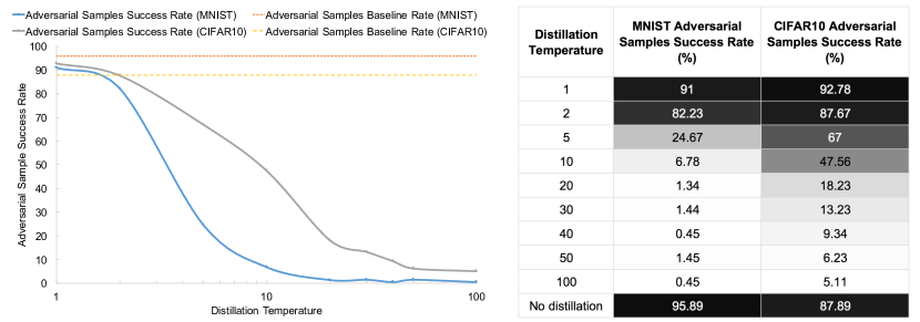
Figure 7: An exploration of the temperature parameter space: for $900$ targets against the MNIST and CIFAR10 based models and several distillation temperatures, we plot the percentage of targets achieved by crafting an adversarial sample while altering at most $112$ features. Baselines for models trained without distillation are in dashes. Note the horizontal logarithmic scale.

V-B Defensive Distillation and Adversarial Samples

Impact on Adversarial Crafting - For each of our two DNN architectures corresponding to the MNIST and CIFAR10 datasets, we consider the original trained model $F_{MNIST}$ or $F_{CIFAR10}$, as well as the distilled model $F^{d}_{MNIST}$ or $F^{d}_{CIFAR10}$. We obtain the two distilled models by training them with defensive distillation at a class knowledge transfer temperature of $T=20$ (the choice of this parameter is investigated below). The resulting classification accuracy for the MNIST model $F^{d}_{MNIST}$ is $99.05\%$ and the classification accuracy for the CIFAR10 model $F^{d}_{CIFAR10}$ is $81.39\%$, which are comparable to the non-distilled models.

In a second set of experiments, we measured success rate of adversarial sample crafting on $100$ samples randomly selected from each dataset. That is, for each considered sample, we use the crafting algorithm to craft $9$ adversarial samples corresponding to the $9$ classes distinct from the sample’ source class. We thus craft a total of $900$ samples for each model. For the architectures trained on MNIST data, we find that using defensive distillation reduces the success rate of adversarial sample crafting from $95.89\%$ for the original model to $1.34\%$ for the distilled model, thus resulting in a $98.6\%$ decrease. Similarly, for the models trained on CIFAR10 data, we find that using distillation reduces the success rate of adversarial sample crafting from $89.9\%$ for the original model to $16.76\%$ for the distilled model, which represents a $81.36\%$ decrease.

Distillation Temperature - The next experiments measure how temperature impacts adversarial sample generation. Note the softmax layer’s temperature is set to $1$ at test time i.e., temperature only matters during training. The objective here is to identify the “optimal” training temperature resulting in resilience to adversarial samples for a DNN and dataset.

We repeat the adversarial sample crafting experiment on both architectures and vary the distillation temperature each time. The number of adversarial targets successfully reached for the following distillation temperatures $T$: $\{1,2,5,10,20,30,50,100\}$ is measured. Figure 7 plots the success rate of adversarial samples with respect to temperature for both architectures and provides exact figures. In other words, the rate plotted is the number of adversarial sample targets that were reached. Two interesting observations can be made: (1) increasing the temperature will generally speaking make adversarial sample crafting harder, and (2) there is an elbow point after which the rate largely remains constant ($\approx 0\%$ for MNIST and $\approx 5\%$ for CIFAR10).

Observation (1) validates analytical results from Section III showing distilled network resilience to adversarial samples: the success rate of adversarial crafting is reduced from $95.89\%$ without distillation to $0.45\%$ with distillation ($T=100$) on the MNIST based DNN, and from $87.89\%$ without distillation to $5.11\%$ with distillation ($T=100$) on the CIFAR10 DNN.

The temperature corresponding to the curve elbow is linked to the role temperature plays within the softmax layer. Indeed, temperature is used to divide logits given as inputs to the softmax layer, in order to provide more discreet or smoother distributions of probabilities for classes. Thus, one can make the hypothesis that the curve’s elbow is reached when the temperature is such that increasing it further would not make the distribution smoother because probabilities are already close to $1/N$ where $N$ is the number of classes. We confirm this hypothesis by computing the average maximum probability output by the CIFAR10 DNN: it is equal to $0.72$ for $T=1$, to $0.14$ for $T=20$, and to $0.11$ for $T=40$. Thus, the elbow point at $T=40$ correspond to probabilities near $1/N=0.1$.

Classification Accuracy - The next set of experiments sought to measure the impact of the approach on accuracy. For each knowledge transfer temperature $T$ used in the previous set of experiments, we compute the variation of classification accuracy between the models $F_{MNIST},F_{CIFAR10}$ and $F^{d}_{MNIST},F^{d}_{CIFAR10}$, respectively trained without distillation and with distillation at temperature $T$. For each model, the accuracy is computed using all $10,000$ samples from the corresponding test set (from MNIST for the first and from CIFAR10 for the second model). Recall that the baseline rate, meaning the accuracy rate corresponding to training performed without distillation, which we computed previously was $99.51\%$ for model $F_{MNIST}$ and $80.95\%$ for model $F_{CIFAR10}$. The variation rates for the set of distillation temperatures are shown in Figure 8.

Figure 8: Influence of distillation on accuracy: we plot the accuracy variations of our two architectures for a training with and without defensive distillation. These rates were evaluated on the corresponding test set for various temperature values.

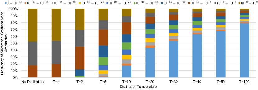
Figure 9: An exploration of the impact of temperature on the amplitude of adversarial gradients: We illustrate how adversarial gradients vanish as distillation is performed at higher temperatures. Indeed, for each temperature considered, we draw the repartition of samples in each of the 10 ranges of mean adversarial gradient amplitudes associated with a distinct color. This data was collected using all $10,000$ samples from the CIFAR10 test set on the corresponding DNN model.

One can observe that variations in accuracy introduced by distillation are moderate. For instance, the accuracy of the MNIST based model is degraded by less than $1.28\%$ for all temperatures, with for instance an accuracy of $99.05\%$ for $T=20$, which would have been state of the art until very recently. Similarly, the accuracy of the CIFAR10 based model is degraded by at most $1.37\%$. It also potentially improves it, as some variations are positive, notably for the CIFAR10 model (the MNIST model is hard to improve because its accuracy is already close to a $100\%$). Although providing a quantitative understanding of this potential for accuracy improvement is outside the scope of this paper, we believe that it stems from the generalization capabilities favored by distillation, as investigated in the analytical study of defensive distillation conducted previously in Section III.

To summarize, not only distillation improves resilience of DNNs to adversarial perturbations (from $95.89\%$ to $0.45\%$ on a first DNN, and from $87.89\%$ to $5.11\%$ on a second DNN), it also does so without severely impacting classification correctness (the accuracy variability between models trained without distillation and with distillation is smaller than $1.37\%$ for both DNNs). Thus, defensive distillation matches the second defense requirement from Section II. When deploying defensive distillation, defenders will have to empirically find a temperature value $T$ offering a good balance between robustness to adversarial perturbations and classification accuracy. In our case, for the MNIST model for instance, such a temperature would be $T=20$ according to Figure 7 and 8.

V-C Distillation and Sensitivity

The second battery of experiments sought to demonstrate the impact of distillation on a DNN’s sensitivity to inputs. Our hypothesis is that our defense mechanism reduces gradients exploited by adversaries to craft perturbations. To confirm this hypothesis, we evaluate the mean amplitude of these gradients on models trained without and with defensive distillation. In this experiment, we split the $10,000$ samples from the CIFAR10 test set into bins according to the mean value of their adversarial gradient amplitude. We train these at varying temperatures and plot the resulting bin frequencies in Figure 9.

Note that distillation reduces the average absolute value of adversarial gradients: for instance the mean adversarial gradient amplitude without distillation is larger than $0.001$ for 4763 samples among the 10,000 samples considered, whereas it is the case only for 172 samples when distillation is performed at a temperature of $T=100$. Similarly, 8 samples are in the bin corresponding to a mean adversarial gradient amplitude smaller than $10^{-40}$ for the model trained without distillation, whereas there is a vast majority of samples, namely 7908 samples, with a mean adversarial gradient amplitude smaller than $10^{-40}$ for the model trained with defensive distillation at a temperature of $T=100$. Generally speaking one can observe that the largest frequencies of samples shifts from higher mean amplitudes of adversarial gradients to smaller ones.

When the amplitude of adversarial gradients is smaller, it means the DNN model learned during training is smoother around points in the distribution considered. This in turns means that evaluating the sensitivity of directions will be more complex and crafting adversarial samples will require adversaries to introduce more perturbation for the same original samples. Another observation is that overtraining does not help because when there is overfitting, the adversarial gradients progressively increase in amplitude so early stopping and other similar techniques can help to prevent exploding. This is further discussed in Section VI. In our case, training for 50 epochs was sufficient for distilled DNN models to achieve comparable accuracies to original models, and ensured that adversarial gradients did not explode. These experiments show that distillation can have a smoothing impact on classification models learned during training. Indeed, gradients characterizing model sensitivity to input variations are reduced by factors larger than $10^{30}$ when defensive distillation is applied.

V-D Distillation and Robustness

Lastly, we explore the interplay between smoothness of classifiers and robustness. Intuitively, robustness is the average minimal perturbation required to produce an adversarial sample from the distribution modeled by $F$.

Figure 10: Quantifying the impact of distillation temperature on robustness: we plot the value of robustness described in Equation 11 for several temperatures and compare it to a baseline robustness value for models trained without distillation.

Robustness - Recall the definition of robustness:

$$\rho_{adv}(F)=E_{\mu}[\Delta_{adv}(X,F)]$$ (10)

where inputs $X$ are drawn from distribution $\mu$ that DNN architecture $F$ is trying to model, and $\Delta_{adv}(X,F)$ is defined in Equation 4 to be the minimum perturbation required to misclassify sample $X$ in each of the other classes. We now evaluate whether distillation effectively increases this robustness metric for our evaluation architectures. To do this without exhaustively searching all perturbations for each possible sample of the underlying distribution modeled by the DNN, we approximate the metric: we compute the metric over all 10,000 samples in the test set for each model. This results in the computation of the following quantity:

$$\rho_{adv}(F)\simeq\frac{1}{|\cal{X}|}\sum_{X\in\cal{X}}\min_{\delta X}\|\delta X\|$$ (11)

where values of $\delta X$ are evaluated by considering each of the 9 possible adversarial targets corresponding to sample $X\in\cal{X}$. and using the number of features altered while creating the corresponding adversarial samples as the distance measure to evaluate the minimum perturbation $\|\delta X\|$ required to create the mentionned adversarial sample. In Figure 10, we plot the evolution of the robustness metric with respect to an increase in distillation temperature for both architectures. One can see that as the temperature increases, the robustness of the network as defined here, increases. For the MNIST architecture, the model trained without distillation displays a robustness of $1.55\%$ whereas the model trained with distillation at $T=20$ displays a robustness of $13.79\%$, an increase of $790\%$. Note that, perturbations of $13.79\%$ are large enough that they potentially change the true class or could be detected by an anomaly detection process. In fact, it was empirically shown in previous work that humans begin to misclassify adversarial samples (or at least identify them as erroneous) for perturbations larger than $13.79\%$: see Figure 16 in [7]. It is not desirable for adversary to produce adversarial samples identifiable by humans. Furthermore, changing additional features can be hard, depending on the input nature. In this evaluation, it is easy to change a feature in the images. However, if the input was spam email, it would become challenging for the adversary to alter many input features. Thus, making DNNs robust to small perturbations is of paramount importance. Similarly, for the CIFAR10 architecture, the model trained without distillations displays a robustness of $0.39\%$ whereas the model trained with defensive distillation at $T=50$ has a robustness of $2.56\%$, which represents an increase of $556\%$. This result suggests that indeed distillation is able to provide sufficient additional knowledge to improve the generalization capabilities of DNNs outside of their training manifold, thus developing their robustness to perturbations.

Distillation and Confidence - Next we investigate the impact of distillation temperature on DNN classification confidence. Our hypothesis is that distillation also impacts the confidence of class predictions made by distilled model.

To test this hypothesis, we evaluate the confidence prediction for all $10,000$ samples in the CIFAR10 dataset. We average the following quantity over all samples $X\in\cal{X}$:

$$C(X)=\left\{\begin{array}[]{c}0\mbox{ if }\arg\max_{i}F_{i}(X)\neq t(X)\\ \arg\max_{i}F_{i}(X)\mbox{ otherwise}\end{array}\right.$$ (12)

where $t(X)$ is the correct class of sample $X$. The resulting confidence values are shown in Table III where the lowest confidence is $0\%$ and the highest $100\%$. The monotonically increasing trend suggests that distillation does indeed increase predictive confidence. Note that a similar analysis of MNIST is inconclusive because all confidence values are already near $99\%$, which leaves little opportunity for improvement.

$T$	1	2	5	10	20
$C(X)$	71.85%	71.99%	78.05%	80.77%	81.06%

TABLE III: CIFAR10 model prediction confidence: $C(X)$ is evaluated on the test set at various temperatures $T$.

VI Discussion

The preceding analysis of distillation shows that it can increase the resilience of DNNs to adversarial samples. Training extracts knowledge learned about classes from probability vectors produced by the DNN. Resulting models have stronger generalizations capabilities outside of their training set.

A limitation of defensive distillation is that it is only applicable to DNN models that produce an energy-based probability distribution, for which a temperature can be defined. Indeed, this paper’s implementation of distillation is dependent on an engergy-based probability distribution for two reasons: the softmax produces the probability vectors and introduces the temperature parameter. Thus, using defensive distillation in machine learning models different from DNNs would require additional research efforts. However note that many machine learning models, unlike DNNs, don’t have the model capacity to be able to resist adversarial examples. For instance, Goodfellow et al. [9] showed that shallow models like linear models are also vulnerable to adversarial examples and are unlikely to be hardened against them. A defense specialized to DNNs, guaranteed by the universal approximation property to at least be able to represent a function that correctly processes adversarial examples, is thus a significant step towards building machine learning models robust to adversarial samples.

In our evaluation setup, we defined the distance measure between original samples and adversarial samples as the number of modified features. There are other metrics suitable to compare samples, like $L1,L2$ norms. Using different metrics will produce different distortions and can be pertinent in application domains different from computer vision. For instance, crafting adversarial samples from real malware to evade existing detection methods will require different metrics and perturbations [16, 37]. Future work should investigate the use of various distance measures.

One question is also whether the probabilities, used to transfer knowledge in this paper, could be replaced by soft class labels. For a $N$-class classification problem, soft labels are obtained by replacing the target value of $1$ for the correct class with a target value of $0.9$, and for the incorrect classes replacing the target of 0 with $\frac{1}{10\cdot N}$. We empirically observed that the improvements to the neural network’s robustness are not as significant with soft labels. Specifically, we trained the MNIST DNN used in Section V using soft labels. The misclassification rate of adversarial samples, crafted using MNIST test data and the same attack parameters than in Section V, was of $86.00\%$, whereas the distilled model studied in Section V had a misclassification rate smaller than $1\%$ We believe this is due to the relative information between classes encoded in probability vectors and not in soft class labels. Inspired by an early public preprint of this paper, Warde-Farley and Goodfellow [38] independently tested label smoothing, and found that it partially resists adversarial examples crafted using the fast gradient sign method [9]. One possible interpretation of these conflicting results is that label smoothing without distillation is smart enough to defend against simple, inexpensive methods [9] of adversarial example crafting but not more powerful iterative methods used in this paper [7].

Future work should also evaluate the performance of defensive distillation in the face of different perturbation types. For instance, while defensive distillation is a good defense against the attack studied here [7], it could still be vulnerable to other attacks based on L-BFGS [8], the fast gradient sign method [9], or genetic algorithms [32]. However, against such techniques, the preliminary results from [38] are promising and worthy of exploration; it seems likely that distillation will also have a beneficial defensive impact with such techniques.

In this paper, we did not compare our defense technique to traditional regularization techniques because adversarial examples are not a traditional overfitting problem [9]. In fact, previous work showed that a wide variety of traditional regularization methods including dropout and weight decay either fail to defend against adversarial examples or only do so by seriously harming accuracy on the original task [8, 9].

Finally, we would like to point out that defensive distillation does not create additional attack vectors, in other words does not start an arms race between defenders and attackers. Indeed, the attacks [8, 9, 7] are designed to be approximately optimal regardless of the targeted model. Even if an attacker knows that defensive distillation is being used, it is not clear how he could exploit this to adapt its attack. By increasing confidence estimates across a lot of the model’s input space, defensive distillation should lead to strictly better models.

VII Related Work

Machine learning security [39] is an active research area in the security community [40]. Attacks have been organized in taxonomies according to adversarial capabilities in [12, 41]. Biggio et al. studied binary classifiers deployed in adversarial settings and proposed a framework to secure them [42]. Their work does not consider deep learning models but rather binary classifiers like Support Vector Machines or logistic regression. More generally, attacks against machine learning models can be partitioned by execution time: during training [43, 44] or at test time [14] when the model is used to make predictions.

Previous work studying DNNs in adversarial settings focused on presenting novel attacks against DNNs at test time, mainly exploiting vulnerabilities to adversarial samples [7, 9, 8]. These attacks were discussed in depth in section II. These papers offered suggestions for defenses but their investigation was left to future work by all authors, whereas we proposed and evaluated a full defense mechanism to improve the resilience of DNNs to adversarial perturbations.

Nevertheless some attempts were made at making DNN resilient to adversarial perturbations. Goodfellow et al. showed that radial basis activation functions are more resistant to perturbations, but deploying them requires important modifications to the existing architecture [9]. Gu et al. explored the use of denoising auto-encoders, a DNN type of architecture intended to capture main factors of variation in the data, and showed that they can remove substantial amounts of adversarial noise [17]. However the resulting stacked architecture can again be evaded using adversarial samples. The authors therefore proposed a new architecture, Deep Contractive Networks, based on imposing layer-wise penalty defined using the network’s Jacobian. This penalty however limits the capacity of Deep Contractive Networks compared to traditional DNNs.

VIII Conclusions

In this work we have investigated the use of distillation, a technique previously used to reduce DNN dimensionality, as a defense against adversarial perturbations. We formally defined defensive distillation and evaluated it on standard DNN architectures. Using elements of learning theory, we analytically showed how distillation impacts models learned by deep neural network architectures during training. Our empirical findings show that defensive distillation can significantly reduce the successfulness of attacks against DNNs. It reduces the success of adversarial sample crafting to rates smaller than $0.5\%$ on the MNIST dataset and smaller than $5\%$ on the CIFAR10 dataset while maintaining the accuracy rates of the original DNNs. Surprisingly, distillation is simple to implement and introduces very little overhead during training. Hence, this work lays out a new foundation for securing systems based on deep learning.

Future work should investigate the impact of distillation on other DNN models and adversarial sample crafting algorithms. One notable endeavor is to extend this approach outside of the scope of classification to other DL tasks. This is not trivial as it requires finding a substitute for probability vectors used in defensive distillation with similar properties. Lastly, we will explore different definitions of robustness that measure other aspects of DNN resilience to adversarial perturbations.

Acknowledgment

The authors would like to thank Damien Octeau, Ian Goodfellow, and Ulfar Erlingsson for their insightful comments. Research was sponsored by the Army Research Laboratory and was accomplished under Cooperative Agreement Number W911NF-13-2-0045 (ARL Cyber Security CRA). The views and conclusions contained in this document are those of the authors and should not be interpreted as representing the official policies, either expressed or implied, of the Army Research Laboratory or the U.S. Government. The U.S. Government is authorized to reproduce and distribute reprints for Government purposes notwithstanding any copyright notation here on.

References

- [1] A. Krizhevsky, I. Sutskever, and G. E. Hinton, “Imagenet classification with deep convolutional neural networks,” in Advances in neural information processing systems, 2012, pp. 1097–1105.
- [2] T. N. Sainath, A.-r. Mohamed, B. Kingsbury, and B. Ramabhadran, “Deep convolutional neural networks for lvcsr,” in Acoustics, Speech and Signal Processing (ICASSP), 2013 IEEE International Conference on. IEEE, 2013, pp. 8614–8618.
- [3] P. Sermanet, D. Eigen, X. Zhang, M. Mathieu, R. Fergus, and Y. LeCun, “Overfeat: Integrated recognition, localization and detection using convolutional networks,” in International Conference on Learning Representations (ICLR 2014). arXiv preprint arXiv:1312.6229, 2014.
- [4] G. E. Dahl, J. W. Stokes, L. Deng, and D. Yu, “Large-scale malware classification using random projections and neural networks,” in Acoustics, Speech and Signal Processing (ICASSP), 2013 IEEE International Conference on. IEEE, 2013, pp. 3422–3426.
- [5] Z. Yuan, Y. Lu, Z. Wang, and Y. Xue, “Droid-sec: deep learning in android malware detection,” in Proceedings of the 2014 ACM conference on SIGCOMM. ACM, 2014, pp. 371–372.
- [6] E. Knorr, “How paypal beats the bad guys with machine learning,” 2015. [Online]. Available: http://www.infoworld.com/article/2907877/machine-learning/how-paypal-reduces-fraud-with-machine-learning.html
- [7] N. Papernot, P. McDaniel, S. Jha, M. Fredrikson, Z. B. Celik, and A. Swami, “The limitations of deep learning in adversarial settings,” in Proceedings of the 1st IEEE European Symposium on Security and Privacy. IEEE, 2016.
- [8] C. Szegedy, W. Zaremba, I. Sutskever, J. Bruna, D. Erhan, I. Goodfellow, and R. Fergus, “Intriguing properties of neural networks,” in Proceedings of the 2014 International Conference on Learning Representations. Computational and Biological Learning Society, 2014.
- [9] I. J. Goodfellow, J. Shlens, and C. Szegedy, “Explaining and harnessing adversarial examples,” in Proceedings of the 2015 International Conference on Learning Representations. Computational and Biological Learning Society, 2015.
- [10] NVIDIA, “Nvidia tegra drive px: Self-driving car computer,” 2015. [Online]. Available: http://www.nvidia.com/object/drive-px.html
- [11] D. Cireşan, U. Meier, J. Masci et al., “Multi-column deep neural network for traffic sign classification.”
- [12] L. Huang, A. D. Joseph, B. Nelson, B. I. Rubinstein, and J. Tygar, “Adversarial machine learning,” in Proceedings of the 4th ACM workshop on Security and artificial intelligence. ACM, 2011, pp. 43–58.
- [13] B. Biggio, G. Fumera et al., “Pattern recognition systems under attack: Design issues and research challenges,” International Journal of Pattern Recognition and Artificial Intelligence, vol. 28, no. 07, p. 1460002, 2014.
- [14] B. Biggio, I. Corona, D. Maiorca, B. Nelson et al., “Evasion attacks against machine learning at test time,” in Machine Learning and Knowledge Discovery in Databases. Springer, 2013, pp. 387–402.
- [15] A. Anjos and S. Marcel, “Counter-measures to photo attacks in face recognition: a public database and a baseline,” in Proceedings of the 2011 International Joint Conference on Biometrics. IEEE, 2011.
- [16] P. Fogla and W. Lee, “Evading network anomaly detection systems: formal reasoning and practical techniques,” in Proceedings of the 13th ACM conference on Computer and communications security. ACM, 2006, pp. 59–68.
- [17] S. Gu and L. Rigazio, “Towards deep neural network architectures robust to adversarial examples,” in Proceedings of the 2015 International Conference on Learning Representations. Computational and Biological Learning Society, 2015.
- [18] J. Ba and R. Caruana, “Do deep nets really need to be deep?” in Advances in Neural Information Processing Systems, 2014, pp. 2654–2662.
- [19] G. Hinton, O. Vinyals, and J. Dean, “Distilling the knowledge in a neural network,” in Deep Learning and Representation Learning Workshop at NIPS 2014. arXiv preprint arXiv:1503.02531, 2014.
- [20] Y. LeCun and C. Cortes, “The mnist database of handwritten digits,” 1998.
- [21] A. Krizhevsky and G. Hinton, “Learning multiple layers of features from tiny images,” 2009.
- [22] Y. Bengio, I. J. Goodfellow, and A. Courville, “Deep learning,” 2015, book in preparation for MIT Press. [Online]. Available: http://www.iro.umontreal.ca/~bengioy/dlbook
- [23] G. E. Hinton, “Learning multiple layers of representation,” Trends in cognitive sciences, vol. 11, no. 10, pp. 428–434, 2007.
- [24] D. E. Rumelhart, G. E. Hinton, and R. J. Williams, “Learning representations by back-propagating errors,” Cognitive modeling, vol. 5, 1988.
- [25] J. Bergstra and Y. Bengio, “Random search for hyper-parameter optimization,” The Journal of Machine Learning Research, vol. 13, no. 1, pp. 281–305, 2012.
- [26] X. Glorot, A. Bordes, and Y. Bengio, “Domain adaptation for large-scale sentiment classification: A deep learning approach,” in Proceedings of the 28th International Conference on Machine Learning (ICML-11), 2011, pp. 513–520.
- [27] J. Masci, U. Meier, D. Cireşan et al., “Stacked convolutional auto-encoders for hierarchical feature extraction,” in Artificial Neural Networks and Machine Learning–ICANN 2011. Springer, 2011, pp. 52–59.
- [28] D. Erhan, Y. Bengio, A. Courville, P.-A. Manzagol, P. Vincent, and S. Bengio, “Why does unsupervised pre-training help deep learning?” The Journal of Machine Learning Research, vol. 11, pp. 625–660, 2010.
- [29] T. Miyato, S. Maeda, M. Koyama et al., “Distributional smoothing by virtual adversarial examples,” CoRR, vol. abs/1507.00677, 2015.
- [30] A. Fawzi, O. Fawzi, and P. Frossard, “Analysis of classifiers’ robustness to adversarial perturbations,” in Deep Learning Workshop at ICML 2015. arXiv preprint arXiv:1502.02590, 2015.
- [31] H. Drucker and Y. Le Cun, “Improving generalization performance using double backpropagation,” Neural Networks, IEEE Transactions on, vol. 3, no. 6, pp. 991–997, 1992.
- [32] A. Nguyen, J. Yosinski, and J. Clune, “Deep neural networks are easily fooled: High confidence predictions for unrecognizable images,” in In Computer Vision and Pattern Recognition (CVPR 2015). IEEE, 2015.
- [33] G. Cybenko, “Approximation by superpositions of a sigmoidal function,” Mathematics of Control, Signals, and Systems , vol. 5, no. 4, p. 455, 1992.
- [34] S. Shalev-Shwartz, O. Shamir, N. Srebro, and K. Sridharan, “Learnability, stability and uniform convergence,” The Journal of Machine Learning Research, vol. 11, pp. 2635–2670, 2010.
- [35] J. Bergstra, O. Breuleux, F. Bastien, P. Lamblin, R. Pascanu, G. Desjardins, J. Turian, D. Warde-Farley, and Y. Bengio, “Theano: a cpu and gpu math expression compiler,” in Proceedings of the Python for scientific computing conference (SciPy), vol. 4. Austin, TX, 2010, p. 3.
- [36] E. Battenberg, S. Dieleman, D. Nouri, E. Olson, A. van den Oord, C. Raffel, J. Schlüter, and S. Kaae Sønderby, “Lasagne: Lightweight library to build and train neural networks in theano,” 2015. [Online]. Available: https://github.com/Lasagne/Lasagne
- [37] B. Biggio, K. Rieck, D. Ariu, C. Wressnegger et al., “Poisoning behavioral malware clustering,” in Proceedings of the 2014 Workshop on Artificial Intelligent and Security Workshop. ACM, 2014, pp. 27–36.
- [38] D. Warde-Farley and I. Goodfellow, “Adversarial perturbations of deep neural networks,” in Advanced Structured Prediction, T. Hazan, G. Papandreou, and D. Tarlow, Eds., 2016.
- [39] M. Barreno, B. Nelson, A. D. Joseph, and J. Tygar, “The security of machine learning,” Machine Learning, vol. 81, no. 2, pp. 121–148, 2010.
- [40] W. Xu, Y. Qi et al., “Automatically evading classifiers,” in Proceedings of the 2016 Network and Distributed Systems Symposium, 2016.
- [41] M. Barreno, B. Nelson, R. Sears, A. D. Joseph, and J. D. Tygar, “Can machine learning be secure?” in Proceedings of the 2006 ACM Symposium on Information, computer and communications security. ACM, 2006, pp. 16–25.
- [42] B. Biggio, G. Fumera, and F. Roli, “Security evaluation of pattern classifiers under attack,” Knowledge and Data Engineering, IEEE Transactions on, vol. 26, no. 4, pp. 984–996, 2014.
- [43] B. Biggio, B. Nelson, and L. Pavel, “Poisoning attacks against support vector machines,” in Proceedings of the 29th International Conference on Machine Learning, 2012.
- [44] B. Biggio, B. Nelson, and P. Laskov, “Support vector machines under adversarial label noise.” in ACML, 2011, pp. 97–112.