Field calculations, single-particle tracking, and beam dynamics with space charge in the electron lens for the Fermilab Integrable Optics Test Accelerator

Abstract

An electron lens is planned for the Fermilab Integrable Optics Test Accelerator as a nonlinear element for integrable dynamics, as an electron cooler, and as an electron trap to study space-charge compensation in rings. We present the main design principles and constraints for nonlinear integrable optics. A magnetic configuration of the solenoids and of the toroidal section is laid out. Single-particle tracking is used to optimize the electron path. Electron beam dynamics at high intensity is calculated with a particle-in-cell code to estimate current limits, profile distortions, and the effects on the circulating beam. In the conclusions, we summarize the main findings and list directions for further work.

I Introduction

Storage rings as well as cyclotrons traditionally rely on the linearity of the particle optics, except where required to correct for effects such as chromaticity. In these machines, the focusing depends linearly on the offset of the particles from the axis and all particles oscillate at approximately the same frequency, the tune. One limit on the intensity of the beam in these machines is the maximum allowable spread of tunes, which is typically limited by the presence of various resonances.

To demonstrate the feasibility of a nonlinear optic in a real machine, the Integrable Optics Test Accelerator (IOTA) ring is being built at Fermilab. The idea is to produce a large tune spread using short nonlinear insertions without reducing the region where beam can be transported stably Danilov and Nagaitsev (2010). The linac of the Fermilab Accelerator Science and Technology (FAST) facility will be used as injector Nagaitsev et al. (2012), generating a $150\text{\,}\mathrm{MeV}$ electron beam.

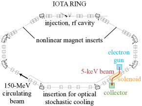
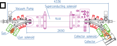
Electron lens in IOTA	Tevatron electron lens (TEL2)

Figure 1: Schematic layout of electron lenses.

Electron lenses can be used to provide the fields required to make the equations of motion integrable and thus non-chaotic. In an electron lens, a low-energy electron beam is guided and compressed by magnetic fields. The profile of this electron beam can be shaped to provide the required kicks to the circulating beam Shiltsev et al. (2008). Electron lenses have been in operation at the Tevatron for compensation of beam-beam effects and abort-gap cleaning Shiltsev et al. (2008) and are considered for a number of other applications such as halo control in LHC Stancari (2014a). Figure 1 (left) shows a schematic layout of the ring, which has a circumference of $40\text{\,}\mathrm{m}$, including the planned electron lens.

The schematic of one of the electron lenses in the Tevatron is shown in Figure 1 (right). The electron beam was produced by an electron gun contained inside a solenoidal magnetic field on a potential of $-5\text{\,}\mathrm{keV}-10\text{\,}\mathrm{keV}$. A short section consisting of three coils provides a magnetic field to guide the electrons into the superconducting main solenoid. An increase in magnetic field from the gun solenoid ($0.3\text{\,}\mathrm{T}$ for TEL) to the main solenoid ($3.1\text{\,}\mathrm{T}$) compresses the electron beam by a factor of $\sqrt{B_{\mathrm{gun}}/B_{\mathrm{main}}}$. The main solenoid included dipole correctors for alignment of the electron beam as well as BPMs. The electron beam was then guided into a collector at a lowered negative potential (to reduce power deposition) by a symmetric set of coils.

For IOTA, two modi of operation are under investigation. In the first case, the electric field of an electron beam of current $I$ with the radially symmetric current density

$$j\!\left(r\right)=\frac{I}{\pi}\frac{a^{2}}{\left(a^{2}+r^{2}\right)^{2}}$$ (1)

generates two invariants of motion making all particle trajectories regular and bounded. A one dimensional system like this was first studied by McMillan and later extended to two dimensions Danilov and Perevedentsev (1997). The electric field and potential of such a distribution with an additional cut-off is listed in Appendix A.

A second option is to use the main solenoid to set the beta function $\beta$ for the circulating beam to a constant value by using a magnetic field of $B_{z}=2\left(B\rho\right)/\beta$. In that case, using any radially symmetric electron beam distribution will conserve the Hamiltonian as well as the longitudinal component of the angular momentum as long as the phase advance in the rest of the ring is a multiple of $\pi$ Stancari (2014a).

Focus of this work is to find an initial design of the bending section, which guides the electron beam into and out of the main solenoid, and to investigate the dynamics of the high current electron beam using particle-in-cell simulation tools Hockney and Eastwood (2010). The beam distribution i.e. its potential and electric field gained from these simulations can then be used as input for long-time tracking simulation of the beam in IOTA.

II Requirements for the bend design

Instead of bending the beam in and out on the same side of the beam line as in TEL2, the IOTA electron lens will feature bending section with different signs of curvature. By doing this, the dipole kicks on the circulating beam during the crossing of the bends should cancel.

For the electron lens in IOTA, it was decided to reuse the electron gun and collector solenoids from TEL2. Their coils have an inner diameter of $25\text{\,}\mathrm{cm}$ and an outer diameter of $47.4\text{\,}\mathrm{cm}$, as well as a length of $30\text{\,}\mathrm{cm}$ Ageev et al. (2001). They can reach a field up to $0.4\text{\,}\mathrm{T}$ on axis. To reach the required compression of the electron beam with a resistive main solenoid however, only $0.1\text{\,}\mathrm{T}$ are required.

An electron energy of $5\text{\,}\mathrm{kV}$ is envisioned and is used throughout this report.

III Geometry of the bending section

The distance of $30\text{\,}\mathrm{cm}$ between the main solenoid and the next IOTA quadrupole leaves little space for the bending solenoids. Thus, the setup from the TEL2 electron lens had to be compressed as much as possible. Figure 2 shows the setup that was used for the following studies. All geometric parameters are summarised in Table 1. The dimensions of the solenoids and coils used are presented in Table 2.

Table 1: Geometric parameters of the initial electron lens bend design.

Center of circle for bending solenoid placement	$z,x$	$40\text{\,}\mathrm{cm}$, $30\text{\,}\mathrm{cm}$
Radius of circle for bending solenoid placement	$R_{\mathrm{bend,sol}}$	$29.56\text{\,}\mathrm{cm}$
Injection angle	$\varphi_{\mathrm{inj}}$	$70\text{\,}\mathrm{\SIUnitSymbolDegree}$
z-axis crossing of straight line from injection	$z_{\mathrm{inj}}$	$64\text{\,}\mathrm{cm}$
Distance between gun and transfer solenoid	$d_{\mathrm{gun,transfer}}$	$7.5\text{\,}\mathrm{cm}$

Table 2: Parameters of the solenoids required for the initial electron lens bend design.

Solenoid	$R_{i}$	$R_{o}$	$B$	$j$	$\Theta$	Center
	[cm]	[cm]	[mT]	$\left[\mathrm{A}/\mathrm{mm}^{2}\right]$	$\left[{}^{\circ}\right]$	[m]
Gun	12.5	23.7	100	1.11	70	(0.517, 0.828)
Transfer	3.5	7.5	100	2.27	70	$r_{\mathrm{trans}}=(0.2114,0.717)$
Bend 1	9.65	13.65	53.9	6.28	43	$r_{\mathrm{bend,1}}=(0.02692,0.682)$
Bend 2	6.33	10.33	74.9	6.28	33.5	$r_{\mathrm{bend,2}}=(0.0118,0.615)$
Bend 3	4.17	8.17	100	6.28	24	$r_{\mathrm{bend,3}}=(0.0,0.5555)$
Main	2.5	10	330	3.53		(0.0, 0.0)

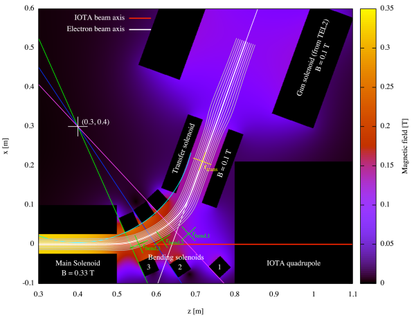
Figure 2: Schematic of an initial bend design for the IOTA electron lens.

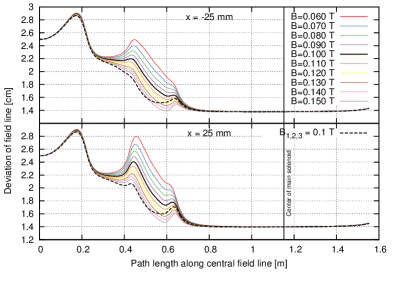
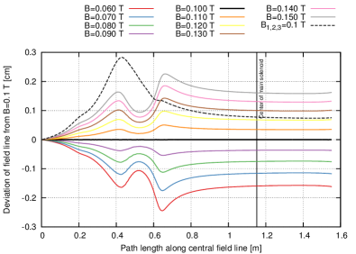
Figure 3: Different settings of the magnetic field of the solenoid in front of the main solenoid. Solid curves for the settings, where the current through all solenoids are equal. Dashed curves for settings with independent setting. Left: Offset of the field lines starting at the gun at $\pm 25\text{\,}\mathrm{mm}$ from the central field line for different settings of the magnetic field. Right: Offset of the central field line compared to the one at $B_{3}=$0.1\text{\,}\mathrm{T}$$.

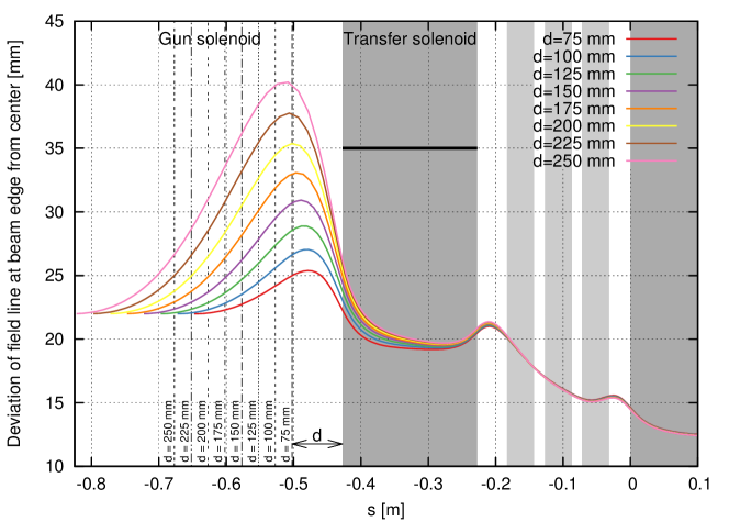
Figure 4: Field line divergence for different distances between gun and transfer solenoid.

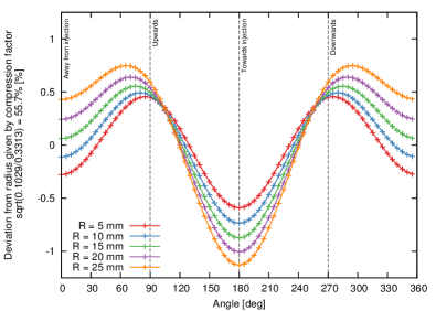
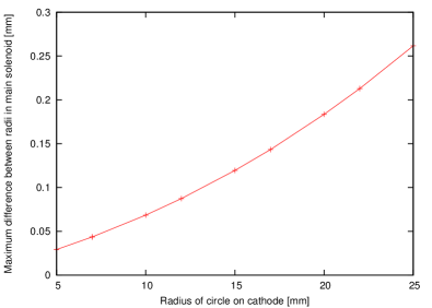
Figure 5: Anisotropy of the magnetic field in the main solenoid. Left: Angular dependency of deformation. Right: Maximal deformation of the field lines.

The design was found using a simple Python code, tracking field lines by numerical integration of

$$\frac{\mathrm{d}\vec{r}}{\mathrm{d}s}=\pm\frac{\vec{B}}{B}\mathrm{.}$$ (2)

For sufficiently large magnetic fields, it can be assumed, that the electron beam will follow these lines with some gyration. The fields of the solenoids were calculated by integrating the Biot-Savart law of cylindrical conductors.

The inner, main solenoid-facing edges of the bending solenoids were arranged on a circle of $R_{\mathrm{bend,sol}}=$29.56\text{\,}\mathrm{cm}$$. The inner diameters of the bending solenoids were chosen, so that the outer, main-solenoid facing edges touch the beam pipe. The origin of the circle as well as the angles at which the three bending solenoids are placed were found by trying to increase field homogeneity in the area of the beam.

To transfer the electron beam from the gun into the bending system an additional solenoid is required. Together with the electron gun, this solenoid was placed on an axis rotated by $\varphi_{\mathrm{inj}}=70^{\circ}$ which crosses the z-axis at $z_{\mathrm{inj}}=$64\text{\,}\mathrm{cm}$$.

Initially the currents through the bending solenoids were set to produce the same field of $0.1\text{\,}\mathrm{T}$ on axis. This, however, led to high current densities of over $>10\text{\,}\mathrm{A}\text{\,}{\mathrm{mm}}^{-2}$ for the first and largest solenoid. To reduce the requirements and stay below the value given as "good" in Ref. Tanabe (2005), the magnets were set to the same current. This reduces the field on axis for the first solenoid to about $54\text{\,}\mathrm{\char 37\relax}$ of the third and that of the second one to about $75\text{\,}\mathrm{\char 37\relax}$, but provides the benefit of operation with just one power supply.

Additionally, reducing the field strength of these solenoids comes at the cost of increased beam radius in the bends, although even at lower field settings the beam should still be well separated from the vacuum chamber. The difference for the outer field lines is shown in Figure 3 (left). In all cases an asymmetry between the inner and outer field lines can be seen in the bending section, which can be as large as $3\text{\,}\mathrm{mm}$. This is a result of the drop of magnetic field towards the center of bending solenoid 1.

Figure 3 (right) shows the deviation of the central field line from the one at $B=$0.1\text{\,}\mathrm{T}$$ for different coil currents. In addition to the difference in beam radii, there is an offset from the axis of the solenoid as well.

In the design, a good way to influence the offset of the field lines in the center of the main solenoid is to change the longitudinal position of injection $z_{\mathrm{inj}}$. Increasing $z_{\mathrm{inj}}$ by a centimeter increases the offset of the central field line by about $2.5\text{\,}\mathrm{mm}$.

The distance $d_{\mathrm{gun,transfer}}$ between the gun and transfer solenoids can easily be increased to fit vacuum equipment. As can be seen in Figure 4, the fields lines bulge out more for increased values in the affected section, but the influence on the bending section is already very small. The maximum distance is thus limited by the available aperture between the solenoids as well as the thickness of the beampipe inside the transfer solenoid. However, there may be additional limits coming from particle drifts and space charge, which will be investigated in the next sections.

To quantify the anisotropy in the field, field lines starting on a circle of radius $R$ around the center of the cathode were tracked to the center of the main solenoid. Assuming a perfectly homogeneous field, the circle should shrink to $\sqrt{B_{gun}/B_{sol}}=\sqrt{0.1/0.33}=$55.0\text{\,}\mathrm{\char 37\relax}$$ of $R$. Stray fields increase the absolute field in the gun to $102.9\text{\,}\mathrm{mT}$ and in the center of the main solenoid to $331.3\text{\,}\mathrm{mT}$. Figure 5 (left) shows the relative deviation of circles of various radii from $\sqrt{102.9/331.3}R=$55.7\text{\,}\mathrm{\char 37\relax}$R$.

The deformation at low radii is mostly quadrupolar in nature. In vertical direction, particles end up at a slightly increased distance from the center, whereas particles in horizontal direction are guided inwards more strongly. There is also a small difference between field lines at positive and negative horizontal offset. The shift in the maxima for higher $R$ is a result of an outwards horizontal shift of the field lines for both positive and negative vertical offsets.

The maximum deviation between field lines for the tracked circles is shown in Figure 5 (right). For the field lines on $R=$25\text{\,}\mathrm{mm}$$ there is significant deformation of up to $0.26\text{\,}\mathrm{mm}$.

IV Single particle tracking

Figure 6: Envelope of a beam with radius $r=$22\text{\,}\mathrm{mm}$$ and no emittance.

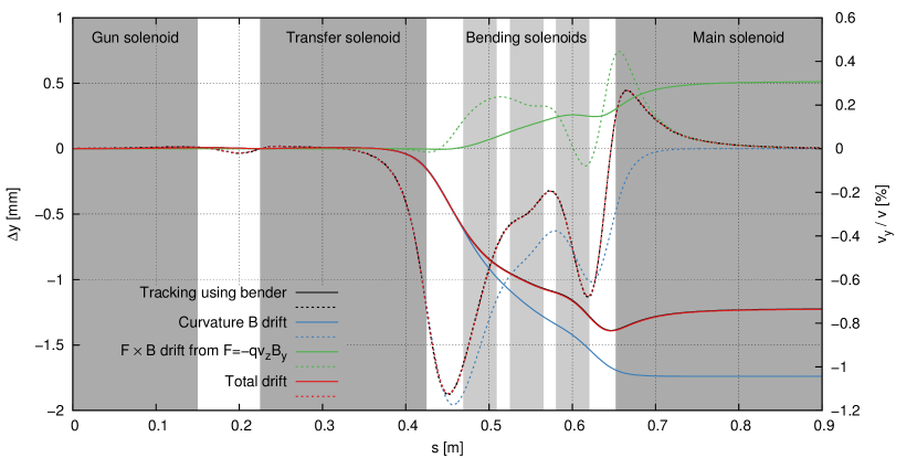
Figure 7: Particle drift along the central field line. Solid lines are vertical offsets, dashed lines are drift velocities. The drift is split in the influence of the curvature drift (blue) and the upward-guiding effect of the vertical magnetic field.

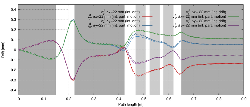
Figure 8: Horizontal and vertical drifts in reference to the central particle. Comparison between field line tracking using eq. 7 ("integrated drift") and integration of motion using bender.

Figure 9: Graphical representation of the distortions of the trajectories in the center of the main solenoid from distortions in the field lines and from particle drifts. Coordinate system is in the reference frame of the electron beam. Dashed lines for particles starting with $r=$22\text{\,}\mathrm{mm}$$ at the cathode.

Single particles were tracked through the system using the particle-in-cell code bender Noll et al. (2014). Time steps of $5\text{\,}\mathrm{ps}$ were used. A comparison with runs using smaller steps of down to $0.5\text{\,}\mathrm{ps}$ showed no significant differences.

To speed up particle tracking the solenoid fields were calculated on an r-z grid with $0.5\text{\,}\mathrm{mm}$ spacing and interpolated to the particle positions. Comparisons to tracking simulations using the full field showed only negligible differences.

Each solenoid contributes significantly to the magnetic field even at large distances and inside the main solenoid. One influence of this is, that the field line at the center of the gun solenoid is pointing at an angle of $\varphi^{\prime}_{\mathrm{inj}}=$70.097\text{\,}\mathrm{\SIUnitSymbolDegree}$$, slightly larger than $\varphi_{\mathrm{inj}}$. For tracking, the source was placed at this modified angle $\varphi^{\prime}_{\mathrm{inj}}$, to minimize the initial magnetic moment of the particles as well as the cyclotron motion. $\varphi^{\prime}_{\mathrm{inj}}$ also varies significantly over the cathode region in horizontal direction, for example increasing linearly from $69.98\text{\,}\mathrm{\SIUnitSymbolDegree}$ to $70.22\text{\,}\mathrm{\SIUnitSymbolDegree}$ in the range of $x=$\pm 22\text{\,}\mathrm{mm}$$.

Furthermore, it was observed that truncating the fields of any of the solenoids inside the simulation volume will have an influence on particle trajectories. Thus, a grid for each magnet spanning the whole system was used.

Figure 6 shows the beam envelope of a $5\text{\,}\mathrm{keV}$ electron beam with negligible emittance. The compression by $55.7\text{\,}\mathrm{\char 37\relax}$, i.e. from $22\text{\,}\mathrm{mm}$ to $12.25\text{\,}\mathrm{mm}$, is equal to the compression of the field lines. The assumption, that the electrons follow the field lines, seems to be fulfilled well. The shift downwards is a result of particle drifts, which will be investigated in the following.

In a magnetic guiding field, when a force acts on a charged particle, it will drift in a direction perpendicular to this force and the magnetic field. The centrifugal force in a bend leads to a curvature drift

$$\vec{v}_{R}=\frac{mv_{\parallel}^{2}}{qR_{c}}\frac{\vec{R}_{c}\times\vec{B}}{B^{2}}\,\mathrm{,}$$ (3)

where $\vec{R}_{c}=\mathrm{d}^{2}\vec{r}/\mathrm{d}s^{2}$ is pointing in the direction of the normal vector along the trajectory and has the magnitude of the radius of a circle that fits the trajectory at each given point. Assuming $\vec{R}$ and $\vec{B}$ to be perpendicular, $B$ pointing only in longitudinal direction and $R$ only in horizontal direction along the particle trajectories, results in a vertical drift. Integrated over path length, the total drift is

$$\Delta y\!\left(s\right)=\frac{2U}{v_{0}}\frac{q}{\left|q\right|}\int_{0}^{s}\mathrm{d}s^{\prime}\frac{1}{R\!\left(s^{\prime}\right)B\!\left(s^{\prime}\right)}\,\mathrm{.}$$ (4)

The curvature B drift was responsible for several millimeters of vertical drift in TEL-1 Shiltsev et al. (2008).

For the design of the bends presented above, the curvature B drift is as large as $1.7\text{\,}\mathrm{mm}$. As the particle moves downwards, it moves into a region where the magnetic field, especially from the main solenoid, is pointing upwards. This vertical field will then guide the particle upwards again. Assuming that particles follow the field lines exactly:

$$\frac{\mathrm{d}y}{\mathrm{d}s}=\frac{B_{y}}{B_{z}}\quad\mathrm{and}\quad\Delta y\!\left(s\right)=\int_{0}^{s}\mathrm{d}s^{\prime}\frac{B_{y}\!\left(s^{\prime}\right)}{B_{z}\!\left(s^{\prime}\right)}$$ (5)

Interestingly, the same equation can also be derived by thinking of the upward movement as an $\vec{F}\times\vec{B}$ drift. The vertical magnetic field produces a force mainly in horizontal direction $F_{x}=-qv_{z}B_{y}$. This force while being negligible in horizontal direction produces a vertical drift, with the velocity

$$v_{y}=\frac{1}{q}\frac{\vec{F}\times\vec{B}}{B^{2}}=-\frac{v_{z}B_{y}B_{z}}{B^{2}}\vec{e}_{x}\times\vec{e}_{z}=v_{z}\frac{B_{y}B_{z}}{B^{2}}\overset{B_{z}\approx B}{=}v_{z}\frac{B_{y}}{B_{z}}\,\mathrm{,}$$ (6)

which is identical to eq. 5.

To follow the drifts along with the field line,

$$\frac{\mathrm{d}\vec{r}}{\mathrm{d}s}=\pm\frac{1}{B}\left\{\vec{B}+\frac{m}{qv_{0}}\frac{1}{B^{2}}\left(v_{||}^{2}+\frac{1}{2}v_{\perp}^{2}\right)\left(\vec{B}\times\vec{\nabla}B\right)\right\}$$ (7)

instead of eq. 2 can be used. The grad B drift can be neglected by setting $v_{\perp}=0$.

The deviation on the central field line resulting from both drifts is plotted in Figure 7. The total offset for the central particle in vertical direction is $-1.2\text{\,}\mathrm{mm}$. The trajectories curvature has two maxima of similar dimensions at the start and the end of the first and the third bending solenoid. Due to the higher magnetic field closer to the main solenoid, the region between transfer and the first bending solenoid accounts for most of the downwards curvature B drift.

For particles with an offset from the central field line, there is an additional drift that is a result from the compression of the beam. On these trajectories $\vec{R}$ is not confined to the bending plane any more, but – in the frame of reference relative to the central field line – also acquires a component pointing radially. Because of $\vec{e}_{r}\times\vec{e}_{z}=-\vec{e}_{\varphi}$, this component causes particles to drift from their position in an angular direction.

Figure 8 shows the drift of particles with an offset of $\pm 22\text{\,}\mathrm{mm}$ in $x$ and $y$ in the perpendicular transverse direction in the frame of reference of the central particle. In the injection part of the system, the field and thus the drift is approximately rotationally symmetrical around the beam axis.

Because there are no differences in absolute field between particles, the drift velocities follow the curvature of the trajectories. Initially, the curvature has a small negative value (radial vector $\vec{R}$ pointing inwards), leading to an initial drift upwards for particles with positive $\Delta x$. About $5\text{\,}\mathrm{cm}$ before the end of the gun solenoid curvature changes sign and increases to about 10 times of the initial value, which results in a much higher drift in the opposing direction. This drift is then reduced because of another change in the sign of the curvature at the start of the transfer solenoid. Most of the drift is canceled in the center of the transport solenoid, only about $\Delta r=$0.05\text{\,}\mathrm{mm}$$ remains.

In the bending section, due to an horizontal gradient in the magnetic field, the magnitude of the vertical drift differs from that in horizontal direction. The qualitative behavior however is still symmetric between the x and y planes, i.e. the drift still follows the curvature produced by the compression of the field lines.

The difference in magnetic field for particles starting with $\pm 22\text{\,}\mathrm{mm}$ horizontal offset can be as high as $50\text{\,}\mathrm{mT}$. This means that the drift produced by the curvature from compression of the field lines will have a smaller influence on particles with negative offset (higher magnetic field) than on those with positive offset. This is visible in Figure 8 in the smaller variation of the (green) curve for the particle with $\Delta x=$-22\text{\,}\mathrm{mm}$$ in comparison to the particle starting with $\Delta x=$22\text{\,}\mathrm{mm}$$ (red curve).

In addition, the horizontal gradient in the magnetic field also changes the total downward drift of the particles. The higher the magnetic field, the lower the drift resulting from the curvature produced by the bending. For this reason, particles on the inner trajectories at higher magnetic field experience a lower total vertical downward drift and thus are moving upwards in reference to the central particle, whereas particles on the outer trajectories are moving downwards. This effect adds to the drift resulting from the compression, producing a larger drift in Figure 8 in vertical direction than in horizontal direction.

Figure 9 summarizes all the distortions of the particle trajectories.

V Beam dynamics with space charge

Apart from providing kicks to the propagating beam in IOTA, the electric field of the electron lens beam also influences the beam itself. To understand the dynamics and estimate the influence of space charge, simulations using bender were made.

bender simulates DC beams by injecting slices of macroparticles into the simulation in every time step. For all simulations presented below, $\Delta t=$5\text{\,}\mathrm{ps}$$ was used. For the electron lens, using 100 particles inserted per step results in a total number of 430k particles. During beam formation, particles at the head of the beam are accelerated away from the particles being injected behind them – to up to 4 times their initial energy. Depending on the beam current, this switch-on effect leads to visible deviation for up to twice the transit time of the beam. For all plots presented here, these particles were discarded.

As an electrostatic code, bender only considers the self electric fields of the beam by computing them numerically from Poissons equation, but neglects the self magnetic fields. This approximation should pose no problem in this case, since the magnetic field produced by the electron beam, for example $B=\mu_{0}I/(2\pi R_{\mathrm{beam}})=$20\text{\,}\mathrm{\SIUnitSymbolMicro T}$$ for $I=$2\text{\,}\mathrm{A}$$ and $R_{\mathrm{beam}}=$2\text{\,}\mathrm{cm}$$, is in the same order of magnitude as earth’s magnetic field and thus much lower than the guiding fields.

The electron gun was not included in the simulation. Instead, the beam was assumed to have the required distribution. The potential on the bounding surface was fixed to the analytic expression of a 2d infinite beam. Since the beam size in the gun solenoid does not vary much, this approximation should be valid. In future simulations however, the electron gun or a distribution from an additional simulation of the gun should be included.

Boundary conditions were set on cylinders at the inner diameters of the coils. For the bend, a tube with a radius of $3\text{\,}\mathrm{cm}$ was put on a circle connecting the end of the transfer solenoid and the start of the main solenoid using CAD software and included using the STL import in bender. The influence of the shape of this pipe should be studied in more detail to provide input for the technical design.

"Low" resolution runs were made using a grid resolution of $1\text{\,}\mathrm{mm}$ grid spacing in all directions ($3.6\text{\times}{10}^{6}$ grid points total) on the Wilson cluster wil (2014). On 16 processors of the amd32 partition, a simulation of 15000 steps took about $20\text{\,}\mathrm{h}$. The processors were distributed by splitting the domain in an upper and lower half and by putting 4 domains on the IOTA beam pipe and 4 following the bends for each half.

"High" resolution runs were made on 192 processors and a grid spacing of $0.5\text{\,}\mathrm{mm}$ ($21.3$ million grid points) at 2500 particles inserted per step (10 million particles in total), taking $9\text{\,}\mathrm{h}$ for 15000 steps on the intel12 partition of Wilson. For these, the parallel particle-grid accumulation routine in bender had to be reimplemented.

V.1 Particle dynamics and current limits

Assuming radial symmetry of the beam, the electric field will only point in radial direction in the absence of compression. An electron which starts with negligible transverse velocity at the cathode will thus be accelerated outwards. However, as the electron gathers transverse momentum, the magnetic force will increase and transfer momentum from the radial direction into the angular direction. After some outward acceleration, the outwards pointing electric and the inwards-pointing magnetic force will equal the centripetal force on the electron. At this point, it will start to move inwards again until it ends up at the radius it started out at, but with a slightly increased angle in respect to the axis.

This motion is the source of the $E\times B$ drift in the angular direction. Looking at the case of a homogeneous beam, its frequency and revolution time are

$$\omega_{E\times B}=\frac{1}{2\pi\epsilon_{0}}\frac{I}{v}\frac{1}{R_{\mathrm{b}}^{2}}\frac{1}{B}\quad\mathrm{and}\quad T=\frac{4\pi^{2}\epsilon_{0}vBR_{\mathrm{b}}^{2}}{I}\mathrm{.}$$ (8)

For a homogeneous beam, the rotation frequency does not depend on $r$ and thus is equal for all particles. Ignoring longitudinal effects, since $R_{\mathrm{b}}\!\left(s\right)=\sqrt{B_{0}/B\!\left(s\right)}R_{0}$, the oscillation frequency is also independent of s, because

$$\omega_{E\times B}=\frac{1}{2\pi\epsilon_{0}}\frac{I}{v}\frac{1}{R_{\mathrm{0}}^{2}}\frac{B\!\left(s\right)}{B_{0}}\frac{1}{B\!\left(s\right)}=\frac{1}{2\pi\epsilon_{0}}\frac{I}{v}\frac{1}{R_{\mathrm{0}}^{2}}\frac{1}{B_{0}}\mathrm{.}$$ (9)

A $2\text{\,}\mathrm{A}$ beam of $2\text{\,}\mathrm{cm}$ radius will rotate with a frequency of only $3.4\text{\,}\mathrm{MHz}$ around its own axis, by approximately $33\text{\,}\mathrm{\SIUnitSymbolDegree}$ from the cathode to the center of the main solenoid. The value as well as the behaviour is matched by the bender simulation by about $1\text{\,}\mathrm{\SIUnitSymbolDegree}$.

The distance an electron at radius $r_{0}$ will travel outwards before it is reflected is given by

$$r=\frac{1}{\epsilon_{0}}\frac{m}{e}\frac{I}{v}\frac{1}{\pi R_{\mathrm{b}}^{2}}\frac{1}{B^{2}}r_{0}\mathrm{.}$$ (10)

For the parameters given above, the deviation of particles at the edge of the beam at the cathode (B=$0.1\text{\,}\mathrm{T}$) is only $49\text{\,}\mathrm{\SIUnitSymbolMicro m}$. Thus, for homogeneous distributions, no significant deformation will occur.

The current limit for a similar system without any bending or beam compression is given by the Brillouin flow limit Davidson (2001),

$$I_{\mathrm{brillouin}}<\frac{1}{2}\frac{e\epsilon_{0}}{m}v_{\mathrm{b}}\pi R_{\mathrm{b}}^{2}B^{2}\approx$410\text{\,}\mathrm{A}$\mathrm{.}$$ (11)

For currents larger than $I_{\mathrm{brillouin}}$, the magnetic force is not able to balance the electric force any more. For a real electron lens, the current is thus only limited by longitudinal effects. Ignoring possible distortions in the beam shape, the individual slowing of particles at different radii as well as the beams emittance, this current limit is given by

$$I<4\pi\epsilon_{0}\sqrt{\frac{e}{m}}U^{3/2}\left(\frac{g_{1}-\sqrt{3g_{2}^{2}-g_{1}^{2}/3}}{4g_{1}^{2}-9g_{2}^{2}}\right)\mathrm{,}$$ (12)

with the geometric factors $g_{1}=\ln\!\left(R_{\mathrm{b}}/R_{\mathrm{p1}}\right)-0.5$ and $g_{2}=\ln\!\left(cR_{\mathrm{b}}/R_{\mathrm{p2}}\right)-0.5$. For derivation of this formula, see Appendix B. For $E_{\mathrm{b}}=$5\text{\,}\mathrm{keV}$$, $c=0.55$, $R_{\mathrm{p1}}=$4\text{\,}\mathrm{cm}$$ and $R_{\mathrm{p2}}=$2.5\text{\,}\mathrm{cm}$$ the current limit is $7.9\text{\,}\mathrm{A}$ ($9.2\text{\,}\mathrm{A}$ from the numerical solution). From the simulation, the current limit for a homogeneous beam of $R_{\mathrm{b}}=$2\text{\,}\mathrm{cm}$$ seems to be between $7.5\text{\,}\mathrm{A}$ and $10\text{\,}\mathrm{A}$. At these currents, a significant build-up of charge somewhere around the transfer solenoid can be observed, which produces a potential large enough to deflect some of the incoming electrons.

For the McMillan case, the rotation frequency depends on the radius,

$$\omega_{E\times B}=\frac{1}{2\pi\epsilon_{0}}\frac{I}{v}\frac{1}{B}\left(1+\frac{a^{2}}{c^{2}}\right)\frac{1}{r^{2}+a^{2}}\mathrm{.}$$ (13)

For the $1.7\text{\,}\mathrm{A}$ case, oscillation frequencies (revolution times) range from $2.4\text{\,}\mathrm{MHz}$ ($417\text{\,}\mathrm{ns}$) on the edge of the beam to $92\text{\,}\mathrm{MHz}$ ($10.9\text{\,}\mathrm{ns}$) near the beam center.

The field in the core of a McMillan distributed beam is also linear, although increased by a factor of $(R_{\mathrm{b}}/a)^{2}+1$ compared to a homogeneously distributed beam with radius $R_{\mathrm{b}}$. For a particle at $r=$1\text{\,}\mathrm{mm}$$ in a $1.7\text{\,}\mathrm{A}$ McMillan distributed beam for example, the excursion predicted by eq. 10 is $200\text{\,}\mathrm{\SIUnitSymbolMicro m}$ or $20\text{\,}\mathrm{\char 37\relax}$. This means, that for the McMillan distribution at high currents some deviation in the profiles can be expected.

V.2 Profiles

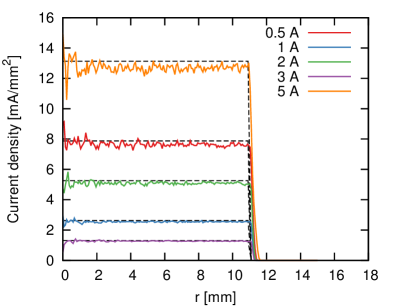
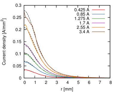
Figure 10: Current density profiles at $z=$30\text{\,}\mathrm{c}\mathrm{m}$$ for various beam currents from the "low resolution" simulation. Left: Homogeneous beam. Right: McMillan distributed beam. The offset from the drift was subtracted before calculation of the current density.

Figure 10 shows the current density profiles in the electron lens. For the homogeneous distribution (left), there is a small systematic dependence of the beam size on the current.

For the McMillan distribution (Figure 10, right), there is a clear deviation from the required profile for the $3.4\text{\,}\mathrm{A}$ simulation: the current density in the core is slightly reduced. The profiles of simulations with lower current follow the theoretical distribution in the tail, but tend to be systematically lower than the theoretical current density around $r=$1\text{\,}\mathrm{mm}$$. In the core of the distribution, there is no systematic behaviour when current increases, probably due to an insufficiently high number of particles close to the axis.

It should be noted, that the grid resolution of the simulation was far below the the deviations seen in these results, making it difficult to draw a final conclusion.

Table 3 contains the deviation of the profiles from the simulations of the transport of the McMillan distributed beam. The rms deviation increase from about 3% for the simulation without space charge to 13% for the visibly distorted profile at $3.4\text{\,}\mathrm{A}$. For the two current values where high resolution simulations where made, the rms values differ by 1.4% ($2\text{\,}\mathrm{A}$) and 0.3% ($3.4\text{\,}\mathrm{A}$) from the lower resolution one respectively. The maximum error values show a significant influence on the resolution of the transport simulation and also don’t increase systematically. It was observed, that changing the resolution on which these errors are calculated significantly changes the value of the residuals.

Table 3: Maximum, arithmetic and rms deviation of the profiles extracted from the simulation to the expected McMillan distribution. The errors were calculated using the same grid resolution used for the high resolution simulation. $N$ is the number of points the current density was calculated on and $j_{0}$ the peak current density.

	$\max(\delta)$	$N^{-1}\sum\delta$	$\sqrt{N^{-1}\sum\delta^{2}}$	$j_{0}^{-1}\max(\delta)$	$j_{0}^{-1}N^{-1}\sum\delta$	$j_{0}^{-1}\sqrt{N^{-1}\sum\delta^{2}}$
	[$\mathrm{kA}\text{\,}{\mathrm{m}}^{-2}$]			[%]
no space charge				3.9	< 0.1	2.9
$0.425\text{\,}\mathrm{A}$	2.9	0.029	1.9	8.3	0.1	5.5
$0.85\text{\,}\mathrm{A}$	7.6	0.069	4.5	10.9	0.1	6.4
$1.275\text{\,}\mathrm{A}$	14.1	0.11	7.3	13.4	0.1	7.0
$1.7\text{\,}\mathrm{A}$	16.7	0.17	10.8	12.0	0.1	7.8
$1.7\text{\,}\mathrm{A}$ (high resolution)	12.1	0.14	9.0	8.7	0.1	6.4
$2.55\text{\,}\mathrm{A}$	26.6	0.31	20.1	12.7	0.1	9.6
$3.4\text{\,}\mathrm{A}$	60.2	0.54	35.2	21.6	0.2	12.6
$3.4\text{\,}\mathrm{A}$ (high resolution)	41.0	0.55	36.1	14.7	0.2	12.9

In Figure 11 the transverse profiles of the electron beam are displayed, showing significant filamentation. This effect is possibly of numerical origin, either from a statistical bias in the original particle distribution or from the influence of the solver grid on the beam, which in these simulations had no emittance. Should fluctuations in the current density in radial direction arise at one point, these would be converted into the observed spiral shape by the dependence of the rotation frequency around the beam center. To understand the origin of the fluctuations, simulations could be made for a simpler system without bending and possibly compression.

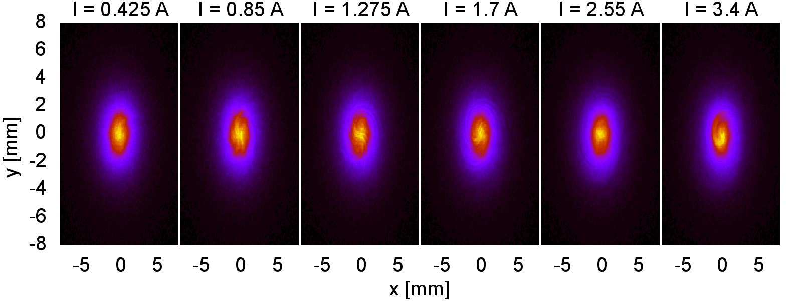
Figure 11: Current profiles at the exit of the simulation volume integrated over time. The electron gun is located towards the positive side of the plot.

V.3 Calculation of kicks on the circulating beam

As described in Ref. Stancari (2014b), the integrated electric field as well as the integrated potential in the area of the electron lens that the circulating beam in IOTA passes can be integrated and fitted using a Chebyshev series. These kick maps can then be used as input for long-term tracking simulations of the beam in IOTA. Using Chebyshev polynomials has the advantage that they are orthogonal, making the resulting coefficients independent, and that they have the same range of values, so that the relative magnitude of the coefficients reflects their weight. Furthermore, it is easy to express the symplecticity condition and to require that the calculated maps are symplectic Stancari (2014b), which is important for long-term tracking.

The integrated potential as well as the kicks (integrated electric fields) are defined as

$$V\!\left(x,y\right)=\int_{z_{0}}^{z_{1}}\mathrm{d}z\,\varphi\!\left(x,y,z\right)\text{ and }k_{i}\!\left(x,y\right)=\int_{z_{0}}^{z_{1}}\mathrm{d}z\,E_{i}\!\left(x,y,z\right)\mathrm{.}$$ (14)

The change in angle of a passing beam particle is then given by $k_{x,y}/(E\rho)$ with the electric rigidity defined as $(E\rho)=pv/e=\gamma m\beta^{2}c^{2}/e$. For a maximum kick $k_{x,w}=$43.35\text{\,}\mathrm{kV}$$ (maximum value in the $1.7\text{\,}\mathrm{A}$ McMillan case), the change in angle is $0.29\text{\,}\mathrm{mrad}$. The potential and the field were calculated using bender on a grid with $0.4\text{\,}\mathrm{mm}$ spacing and then integrated over $z_{0}=$30\text{\,}\mathrm{cm}$$ to $z_{1}=$90\text{\,}\mathrm{cm}$$ using the trapezoidal rule in a range of $\pm a_{x}$ and $\pm a_{y}$ around the central trajectory at $x=$42\text{\,}\mathrm{\SIUnitSymbolMicro m}$$ and $y=$1.22\text{\,}\mathrm{mm}$$, $a_{x}=a_{y}=$1.2\text{\,}\mathrm{cm}$$. The particle distributions from the "high" resolution transport simulations were used.

The expansion of the integrated potential is defined as

$$V\!\left(x,y\right)=\sum_{n=0}^{N}\sum_{j=0}^{n}C_{j,(n-j)}T_{j}\!\left(\frac{x}{a_{x}}\right)T_{n-j}\!\left(\frac{y}{a_{y}}\right)\mathrm{.}$$ (15)

The $T_{j}$ are the Chebyshev polynomials of first kind and $N$ the chosen order of expansion. The kicks can be calculated from the derivatives of $V\!\left(x,y\right)$:

$$k_{x}\!\left(x,y\right)=-\frac{\partial V}{\partial x}=-\frac{1}{a_{x}}\sum_{n=0}^{N}\sum_{j=0}^{n}C_{j,(n-j)}T_{j}^{\prime}\!\left(\frac{x}{a_{x}}\right)T_{n-j}\!\left(\frac{y}{a_{y}}\right)$$

$$k_{y}\!\left(x,y\right)=-\frac{\partial V}{\partial y}=-\frac{1}{a_{y}}\sum_{n=0}^{N}\sum_{j=0}^{n}C_{j,(n-j)}T_{j}\!\left(\frac{x}{a_{x}}\right)T_{n-j}^{\prime}\!\left(\frac{y}{a_{y}}\right)$$

For the derivatives of the Chebyshev polynomials $T_{j}^{\prime}\!\left(x\right)$, the relation

$$T_{n}^{\prime}\!\left(x\right)=nU_{n-1}\!\left(x\right)=n\begin{cases}2\sum_{j\text{ odd}}^{n-1}T_{j}\!\left(x\right)&n-1\text{ odd}\\ 2\sum_{j\text{ even}}^{n-1}T_{j}\!\left(x\right)-1&n-1\text{ even}\end{cases}$$ (16)

was used to avoid numerical problems at $x=0$ that occur in other definitions.

Fits were then made using singular value decomposition of the Vandermonde matrix, fitting either only the integrated potentials $V\!\left(x,y\right)$ or the integrated potential as well as the kicks calculated from the electric field from the bender simulation.

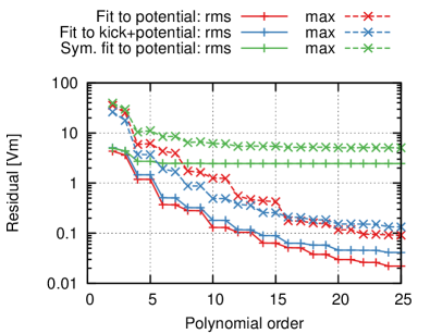
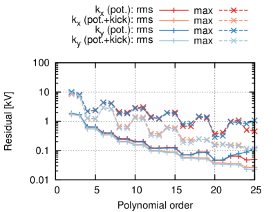
Residuals of the integrated potentials	Residuals of the kicks

Figure 12: Errors in the fits vs. the maximum order of expansion. Top plots: homogeneous distribution; total ranges of values: $V_{w}=$341.9\text{\,}\mathrm{V}\text{\,}\mathrm{m}$$, $k_{x,w}=$19.73\text{\,}\mathrm{kV}$$, $k_{y,w}=$19.0\text{\,}\mathrm{kV}$$. Bottom plots: McMillan distribution; total ranges of values: $V_{w}=$496.8\text{\,}\mathrm{V}\text{\,}\mathrm{m}$$, $k_{x,w}=$43.35\text{\,}\mathrm{kV}$$, $k_{y,w}=$39.7\text{\,}\mathrm{kV}$$.

Table 4: Coefficients $C_{i,j}$ in V$\cdot$m, $a_{x}=a_{y}=$1.2\text{\,}\mathrm{cm}$$ for a homogeneous beam, $R_{\mathrm{b,gun}}=$2\text{\,}\mathrm{cm}$$, $I=$2\text{\,}\mathrm{A}$$

	$T_{0}\!\left(y/a_{y}\right)$	$T_{1}\!\left(y/a_{y}\right)$	$T_{2}\!\left(y/a_{y}\right)$	$T_{3}\!\left(y/a_{y}\right)$	$T_{4}\!\left(y/a_{y}\right)$	$T_{5}\!\left(y/a_{y}\right)$	$T_{6}\!\left(y/a_{y}\right)$	$T_{7}\!\left(y/a_{y}\right)$	$T_{8}\!\left(y/a_{y}\right)$	$T_{9}\!\left(y/a_{y}\right)$	$T_{10}\!\left(y/a_{y}\right)$	$T_{11}\!\left(y/a_{y}\right)$	$T_{12}\!\left(y/a_{y}\right)$	$T_{13}\!\left(y/a_{y}\right)$
$T_{0}\!\left(x/a_{x}\right)$	-2.28e+02	-4.21e+01	4.58e+01	1.44e+00	-2.11e+00	8.84e-03	-1.23e-01	-6.60e-03	-1.12e-02	5.87e-03	-9.89e-03	-2.42e-03	3.64e-04	-2.22e-04
$T_{1}\!\left(x/a_{x}\right)$	-4.31e+00	-4.02e-01	-2.90e-01	2.07e-02	1.15e-02	-7.69e-03	9.98e-03	-4.34e-03	-4.78e-03	4.82e-03	-1.65e-04	-1.70e-03	2.70e-03	2.40e-04
$T_{2}\!\left(x/a_{x}\right)$	5.23e+01	6.19e+00	-9.63e+00	1.42e-01	-1.52e+00	-6.54e-02	3.66e-01	-2.17e-02	8.51e-02	3.85e-04	-9.08e-04	1.55e-03	3.47e-03	1.06e-03
$T_{3}\!\left(x/a_{x}\right)$	-1.03e-01	9.66e-03	-1.65e-02	-1.20e-02	2.17e-02	-4.09e-04	-5.70e-04	1.58e-03	-3.60e-03	-1.34e-03	7.80e-04	3.65e-04	-1.91e-04	-3.28e-04
$T_{4}\!\left(x/a_{x}\right)$	-2.20e+00	9.26e-02	-1.46e+00	-9.78e-02	7.27e-01	-3.81e-02	2.81e-01	2.64e-03	-1.15e-01	1.10e-02	-3.51e-02	-2.31e-04	1.42e-03	-1.28e-03
$T_{5}\!\left(x/a_{x}\right)$	-5.97e-03	4.76e-03	8.19e-03	-8.19e-03	1.46e-02	-1.62e-03	-1.30e-02	5.81e-03	2.02e-03	-2.07e-03	2.33e-03	3.32e-04	-1.06e-03	-5.20e-05
$T_{6}\!\left(x/a_{x}\right)$	-1.30e-01	-3.80e-02	3.43e-01	-2.23e-02	2.60e-01	5.90e-03	-2.01e-01	1.93e-02	-8.05e-02	-4.92e-03	4.02e-02	-2.38e-03	1.56e-02
$T_{7}\!\left(x/a_{x}\right)$	1.08e-03	-4.96e-03	5.84e-03	6.41e-03	-7.49e-03	1.09e-03	-7.44e-04	-2.20e-03	3.89e-03	6.33e-04	-1.44e-03	-7.66e-05
$T_{8}\!\left(x/a_{x}\right)$	-8.86e-03	-1.05e-03	6.21e-02	6.40e-03	-1.00e-01	7.77e-03	-7.52e-02	-4.97e-03	7.11e-02	-1.48e-03	5.71e-0
$T_{9}\!\left(x/a_{x}\right)$	-2.34e-03	1.47e-05	1.59e-03	-1.10e-03	-9.48e-04	2.86e-04	1.62e-03	7.25e-04	-1.03e-03	-6.64e-04
$T_{10}\!\left(x/a_{x}\right)$	-8.27e-03	1.90e-04	5.55e-03	1.24e-03	-3.15e-02	-1.46e-03	3.35e-02	-1.14e-03	6.21e-03
$T_{11}\!\left(x/a_{x}\right)$	7.64e-04	2.69e-03	-1.86e-03	-2.67e-03	1.39e-05	5.73e-04	1.46e-03	-6.44e-04
$T_{12}\!\left(x/a_{x}\right)$	-4.92e-04	4.25e-04	-4.45e-04	-6.61e-04	9.31e-06	-3.52e-04	1.54e-02
$T_{13}\!\left(x/a_{x}\right)$	1.69e-03	-2.05e-03	-6.92e-04	2.52e-03	-3.02e-05	-1.22e-04				$T_{14}\!\left(y/a_{y}\right)$	$T_{15}\!\left(y/a_{y}\right)$	$T_{16}\!\left(y/a_{y}\right)$	$T_{17}\!\left(y/a_{y}\right)$	$T_{18}\!\left(y/a_{y}\right)$
$T_{14}\!\left(x/a_{x}\right)$	2.38e-03	-4.44e-05	1.43e-03	-1.80e-04	6.50e-03				$T_{0}\!\left(x/a_{x}\right)$	1.84e-03	1.26e-03	6.57e-04	-9.98e-04	4.88e-04
$T_{15}\!\left(x/a_{x}\right)$	-1.51e-03	2.01e-03	1.17e-03	-8.09e-04					$T_{1}\!\left(x/a_{x}\right)$	-2.67e-03	3.35e-04	9.77e-04	-3.50e-04
$T_{16}\!\left(x/a_{x}\right)$	8.49e-05	-2.88e-04	-2.36e-03						$T_{2}\!\left(x/a_{x}\right)$	2.85e-04	-7.49e-04	-3.76e-03
$T_{17}\!\left(x/a_{x}\right)$	2.60e-04	-1.10e-03							$T_{3}\!\left(x/a_{x}\right)$	3.10e-04	3.91e-04
$T_{18}\!\left(x/a_{x}\right)$	4.15e-04								$T_{4}\!\left(x/a_{x}\right)$	5.94e-03

Table 5: Coefficients $C_{i,j}$ in V$\cdot$m, $a_{x}=a_{y}=$1.2\text{\,}\mathrm{cm}$$ for a McMillan beam, $a_{\mathrm{gun}}=$3.6\text{\,}\mathrm{mm}$$, $R_{\mathrm{b,gun}}=$2.2\text{\,}\mathrm{cm}$$, $I=$1.7\text{\,}\mathrm{A}$$

	$T_{0}\!\left(y/a_{y}\right)$	$T_{1}\!\left(y/a_{y}\right)$	$T_{2}\!\left(y/a_{y}\right)$	$T_{3}\!\left(y/a_{y}\right)$	$T_{4}\!\left(y/a_{y}\right)$	$T_{5}\!\left(y/a_{y}\right)$	$T_{6}\!\left(y/a_{y}\right)$	$T_{7}\!\left(y/a_{y}\right)$	$T_{8}\!\left(y/a_{y}\right)$	$T_{9}\!\left(y/a_{y}\right)$	$T_{10}\!\left(y/a_{y}\right)$	$T_{11}\!\left(y/a_{y}\right)$	$T_{12}\!\left(y/a_{y}\right)$	$T_{13}\!\left(y/a_{y}\right)$
$T_{0}\!\left(x/a_{x}\right)$	-2.08e+02	-4.22e+01	5.62e+01	3.89e+00	-1.08e+01	-1.01e+00	3.43e+00	4.03e-01	-1.43e+00	-1.81e-01	6.30e-01	1.06e-01	-3.53e-01	-5.11e-02
$T_{1}\!\left(x/a_{x}\right)$	-2.82e+00	-1.54e-01	-8.85e-01	-1.09e-01	2.34e-01	4.38e-02	-7.83e-02	-1.88e-02	2.53e-02	6.64e-03	-1.58e-02	-3.26e-03	5.96e-03	6.22e-04
$T_{2}\!\left(x/a_{x}\right)$	6.82e+01	1.41e+01	-3.62e+01	-3.57e+00	1.30e+01	1.42e+00	-5.41e+00	-6.44e-01	2.40e+00	3.48e-01	-1.25e+00	-1.68e-01	5.78e-01	1.13e-01
$T_{3}\!\left(x/a_{x}\right)$	-7.10e-01	-1.08e-01	7.43e-01	1.28e-01	-3.21e-01	-7.19e-02	1.34e-01	3.55e-02	-6.77e-02	-1.93e-02	2.79e-02	8.08e-03	-1.77e-02	-4.18e-03
$T_{4}\!\left(x/a_{x}\right)$	-1.39e+01	-3.63e+00	1.34e+01	1.57e+00	-6.89e+00	-8.09e-01	3.45e+00	4.61e-01	-1.85e+00	-2.41e-01	9.01e-01	1.65e-01	-5.71e-01	-7.89e-02
$T_{5}\!\left(x/a_{x}\right)$	3.32e-01	5.92e-02	-4.82e-01	-9.17e-02	2.57e-01	6.01e-02	-1.42e-01	-3.62e-02	6.69e-02	1.87e-02	-4.40e-02	-1.14e-02	2.07e-02	4.70e-03
$T_{6}\!\left(x/a_{x}\right)$	4.50e+00	1.29e+00	-5.68e+00	-6.98e-01	3.50e+00	4.57e-01	-2.14e+00	-2.69e-01	1.15e+00	1.96e-01	-7.66e-01	-9.07e-02	3.39e-01
$T_{7}\!\left(x/a_{x}\right)$	-1.85e-01	-3.13e-02	2.89e-01	5.48e-02	-1.94e-01	-4.42e-02	1.06e-01	2.66e-02	-7.34e-02	-1.85e-02	3.18e-02	7.85e-03
$T_{8}\!\left(x/a_{x}\right)$	-1.87e+00	-5.16e-01	2.54e+00	3.43e-01	-1.89e+00	-2.27e-01	1.16e+00	1.86e-01	-8.47e-01	-9.19e-02	3.83e-01
$T_{9}\!\left(x/a_{x}\right)$	1.01e-01	1.41e-02	-1.90e-01	-3.46e-02	1.19e-01	2.70e-02	-9.30e-02	-2.18e-02	4.13e-02	9.90e-03
$T_{10}\!\left(x/a_{x}\right)$	8.28e-01	2.46e-01	-1.32e+00	-1.52e-01	9.22e-01	1.41e-01	-7.71e-01	-8.10e-02	3.84e-01
$T_{11}\!\left(x/a_{x}\right)$	-6.79e-02	-9.52e-03	1.04e-01	1.86e-02	-9.33e-02	-1.99e-02	4.66e-02	1.03e-02
$T_{12}\!\left(x/a_{x}\right)$	-4.46e-01	-1.09e-01	6.09e-01	8.68e-02	-5.79e-01	-6.22e-02	3.42e-01
$T_{13}\!\left(x/a_{x}\right)$	3.49e-02	3.89e-03	-7.72e-02	-1.34e-02	4.66e-02	9.27e-03				$T_{14}\!\left(y/a_{y}\right)$	$T_{15}\!\left(y/a_{y}\right)$	$T_{16}\!\left(y/a_{y}\right)$	$T_{17}\!\left(y/a_{y}\right)$	$T_{18}\!\left(y/a_{y}\right)$
$T_{14}\!\left(x/a_{x}\right)$	2.09e-01	5.83e-02	-3.66e-01	-4.13e-02	2.70e-01				$T_{0}\!\left(x/a_{x}\right)$	1.65e-01	3.31e-02	-9.67e-02	-2.18e-02	6.45e-02
$T_{15}\!\left(x/a_{x}\right)$	-2.55e-02	-2.94e-03	4.17e-02	6.96e-03					$T_{1}\!\left(x/a_{x}\right)$	-2.63e-03	-1.34e-04	3.21e-03	5.97e-04
$T_{16}\!\left(x/a_{x}\right)$	-1.19e-01	-3.01e-02	1.91e-01						$T_{2}\!\left(x/a_{x}\right)$	-3.55e-01	-6.03e-02	1.88e-01
$T_{17}\!\left(x/a_{x}\right)$	1.69e-02	2.80e-03							$T_{3}\!\left(x/a_{x}\right)$	1.02e-02	2.21e-03
$T_{18}\!\left(x/a_{x}\right)$	7.26e-02								$T_{4}\!\left(x/a_{x}\right)$	2.67e-01

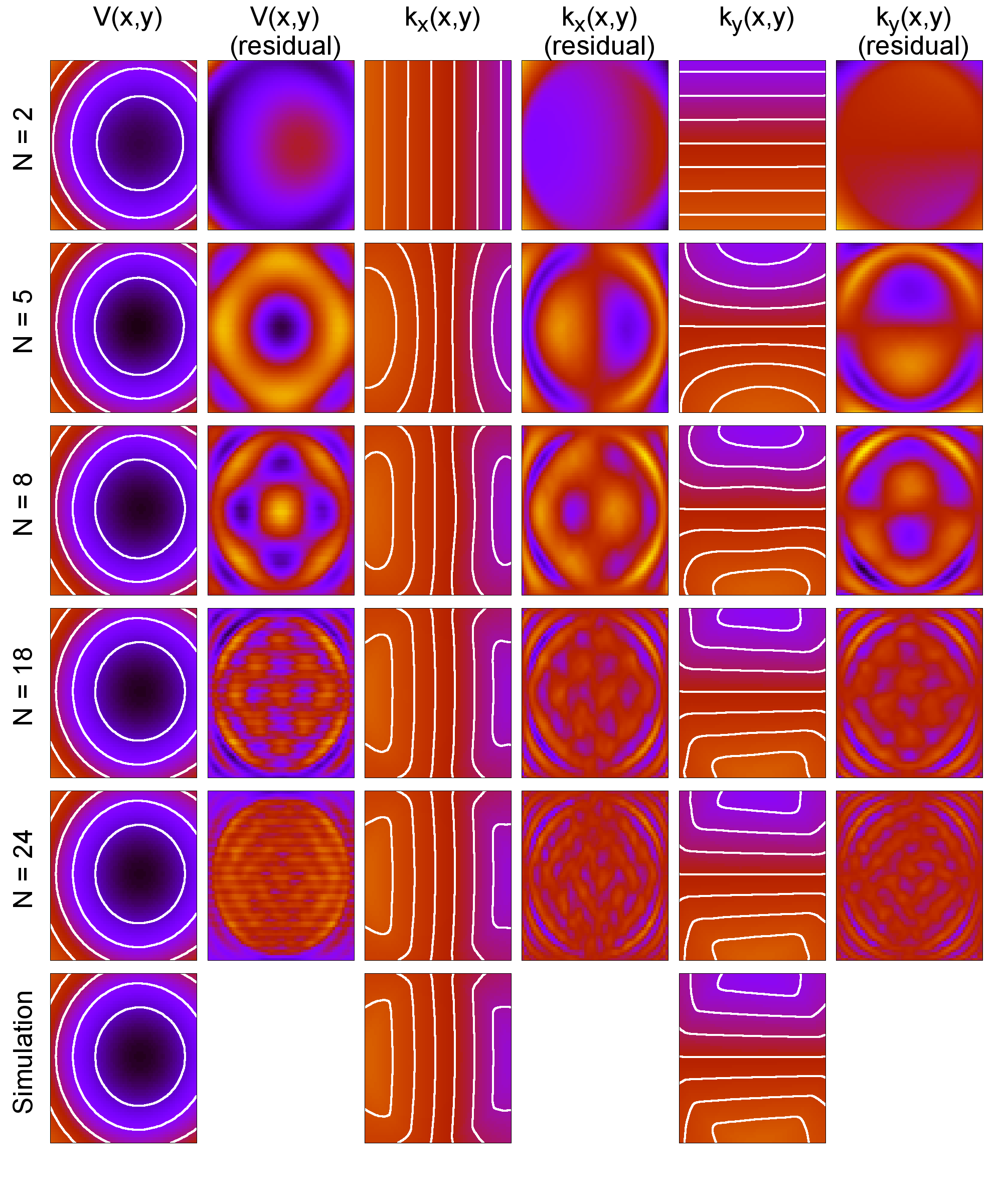
Figure 13: Integrated potentials and kicks and their residual compared to the original data from the simulation for various orders of expansion for the homogeneous beam. The parameters were calculated by fitting the integrated potential and the kicks. Contour line in the plots of the integrated potential range decrease from $-150\text{\,}\mathrm{V}\text{\,}\mathrm{m}-300\text{\,}\mathrm{V}\text{\,}\mathrm{m}$ from the edge of the plots to the center. For the kicks, adjacent lines have a difference of $5\text{\,}\mathrm{kV}$. The lines in the center are at $0\text{\,}\mathrm{V}$.

Figure 14: Integrated potentials and kicks and their residual compared to the original data from the simulation for various orders of expansion for a $1.7\text{\,}\mathrm{A}$, $a=$3.6\text{\,}\mathrm{mm}$$ McMillan distributed beam. The parameters were calculated by fitting the integrated potential and the kicks. Contour line in the plots of the integrated potential range decrease from $-100\text{\,}\mathrm{V}\text{\,}\mathrm{m}-400\text{\,}\mathrm{V}\text{\,}\mathrm{m}$ from the edge of the plots to the center. For the kicks, adjacent lines have a difference of $10\text{\,}\mathrm{kV}$. The lines in the center are at $0\text{\,}\mathrm{V}$.

In Ref. Stancari (2014b), only the coefficients $C_{i,j}$, $j$ even are fitted under the assumption that there is no vertical distortion of the beam. As seen in section IV, the total downward drift of a particle depends on its horizontal position. Thus, since the beam is not completely symmetric, the fit using only even powers in vertical direction fails to provide a good fit. This can be seen from the green curves in Figure 12 (left column). For the homogeneous distribution the effect is much more pronounced, probably due being less peaked than the McMillan distribution.

As was observed in Ref. Stancari (2014b), only fitting the integrated potential values does not sufficiently constrain the derivatives. At higher order, significant oscillation of the calculated kicks can be observed. For the McMillan distribution, no convergence can be observed in Figure 12 (bottom right).

For the homogenous distribution, for $N>18$ there is only little change in the residuals. This is not the case for the McMillan distribution, where the residuals continue to decrease. The reason for this becomes apparent when looking at the distribution of the residuals in Figure 14, which shows a clear maximum in the residuals at the center of the beam. Due to the peaked nature of the McMillan distribution, it takes higher contributions of higher order polynomials to follow the peak of the distribution.

For the values of the constants $C_{i,j}$ for the fit to both potential and kicks to the order $N=18$ please refer to Tables 4 and 5.

VI Conclusion and outlook

A design of the bending sections of the IOTA electron lens was found using field line tracking. The sources of distortions from the magnetic field configuration itself as well as from drifts were investigated. If the total downward drift is canceled and the beam recentered on the axis, the effects are in range of $100\text{\,}\mathrm{\SIUnitSymbolMicro m}$. Including space charge forces, will result in an $E\times B$ motion of the particles. Its behaviour as well as limits from transverse and longitudinal forces were estimated. Space charge calculations were then made using bender, which showed significant change in the profiles at higher currents. Kick maps calculated from the potential and the electric field from these simulations can now be included into tracking simulations to investigate the influence of the asymmetric kicks produced by the bends.

A number of improvements to the simulation as well as open questions are:

• Include the electron gun or use a distribution generated from an external simulation of the electron gun to study how well the required distributions can be approximated and how the differences influence the transport through the electron lens.

• Parameterize various possible aberrations in the electron beam and look into their influence on the beam transport.

• Add the main field and the collector part of the lens to check for a good transport of the beam.

• Investigate the influence of geometry of the beam pipe in the bend on the kicks on the circulating beam and on electron beam transport.

• How large is the magnetic flux from the solenoids into the adjacent quadrupoles of IOTA?

Appendix A Electric field and potential of McMillan distributed beam

Density (cut off at $R_{\mathrm{b}}$):

$$\rho\!\left(r\right)=\frac{a^{4}}{\left(r^{2}+a^{2}\right)^{2}}\theta\!\left(r-R_{\mathrm{b}}\right)$$ (17)

Radial integral:

$$\int_{0}^{r}\mathrm{d}r^{\prime}r^{\prime}\rho\!\left(r^{\prime}\right)=-\frac{a^{4}}{2}\int_{0}^{r}\mathrm{d}r^{\prime}\frac{\mathrm{d}}{\mathrm{d}r^{\prime}}\frac{1}{r^{\prime 2}+a^{2}}=\frac{a^{2}}{2}\left(1-\frac{a^{2}}{r^{2}+a^{2}}\right)=\frac{a^{2}}{2}\frac{r^{2}}{r^{2}+a^{2}}$$ (18)

Cumulative probability density:

$$f\!\left(r\right) =\frac{\int_{0}^{r}\mathrm{d}r^{\prime}\rho\!\left(r^{\prime}\right)}{\int_{0}^{R}\mathrm{d}r^{\prime}\rho\!\left(r^{\prime}\right)}$$

$$=\left(1+\frac{a^{2}}{c^{2}}\right)\frac{r^{2}}{r^{2}+a^{2}}\xrightarrow{c\rightarrow\infty}1-\frac{a^{2}}{r^{2}+a^{2}}=1-\sqrt{\rho\!\left(r\right)}$$

Charge density (beam current $I$, velocity $v$):

$$\rho\!\left(r\right)=\frac{I}{v}\frac{1}{\pi}\left(1+\frac{a^{2}}{R_{\mathrm{b}}^{2}}\right)\frac{a^{2}}{\left(r^{2}+a^{2}\right)^{2}}\theta\!\left(r-R_{\mathrm{b}}\right)$$ (19)

Electric field (aperture $R$):

$$E_{r}\!\left(r\right)=\frac{\rho_{0}}{\epsilon_{0}}\frac{1}{r}\int_{0}^{r}\mathrm{d}r^{\prime}r^{\prime}\rho\!\left(r^{\prime}\right)=\frac{1}{2\pi\epsilon_{0}}\frac{I}{v}\begin{cases}\left(1+\frac{a^{2}}{R_{\mathrm{b}}^{2}}\right)\frac{r}{r^{2}+a^{2}}&r\leq R_{\mathrm{b}}\\ \frac{1}{r}&R_{\mathrm{b}}\leq r<R\end{cases}$$ (20)

Potential:

$$\varphi\!\left(r\right) =-\frac{1}{2\pi\epsilon_{0}}\frac{I}{v}\begin{cases}\ln\!\left(\frac{R_{\mathrm{b}}}{R}\right)+\frac{1}{2}\left(1+\frac{a^{2}}{R_{\mathrm{b}}^{2}}\right)\ln\!\left(\frac{a^{2}+r^{2}}{a^{2}+R_{\mathrm{b}}^{2}}\right)&r\leq R_{\mathrm{b}}\\ \ln\!\left(\frac{r}{R}\right)&R_{\mathrm{b}}\leq r<R\end{cases}$$

Appendix B Current limit during compression of a magnetised beam due to longitudinal space charge forces

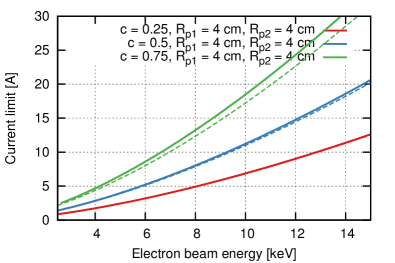
Figure 15: Results of the simple current limit model. Left: Energy dependence. Right: Current limit for different compression values at various beam pipe radii. The solid curves are the results from the numerical solution of the exact equation, the dashed lines are results from the approximation.

If the Brillouin flow limit is sufficiently high, particle drifts, additional distortions due to the magnetic field and the oscillation due to the electric field are low, it can be assumed that the distribution of a beam stays fixed during compression. For a homogeneous, negatively charged beam with current $I$, velocity $v$ and radius $R_{\mathrm{b}}$ in a beam pipe of radius $R_{\mathrm{p}}$,

$$\varphi\!\left(r\right)=\frac{1}{2\pi\epsilon_{0}}\frac{I}{v}\left[\ln\!\left(\frac{R_{\mathrm{b}}}{R_{\mathrm{p}}}\right)-\frac{1}{2}\left(1-\left(\frac{r}{R_{\mathrm{b}}}\right)^{2}\right)\right]$$ (21)

During compression by a factor of $c<1$ from point 1 to 2, the total energy of each particle must be conserved, i.e.

$$0 =E_{2}-E_{1}=\frac{1}{2}mv_{2}^{2}-E_{1}+e\left(\varphi\!\left(r,R_{\mathrm{b}}\right)-\varphi\!\left(cr,cR_{\mathrm{b}}\right)\right)$$

$$\longrightarrow v_{2}^{3}+\left[\frac{eI}{m\pi\epsilon_{0}}g\!\left(r,R_{\mathrm{b}},R_{\mathrm{p,1}}\right)\frac{1}{v_{1}}-\frac{2E_{1}}{m}\right]v_{2}-\frac{eI}{m\pi\epsilon_{0}}g\!\left(cr,cR_{\mathrm{b}},R_{\mathrm{p,2}}\right)=0$$ (22)

with a geometric factor

$$g\!\left(r,R_{\mathrm{b}},R_{\mathrm{p}}\right)=\ln\!\left(\frac{R_{\mathrm{b}}}{R_{\mathrm{p,1}}}\right)-\frac{1}{2}\left(1-\left(\frac{r}{R_{\mathrm{b}}}\right)^{2}\right)\mathrm{,}$$ (23)

which depends on the beam size $R_{\mathrm{b}}$ as well as the radius $R_{\mathrm{p}}$ at which the beam pipe is placed. Equation (22) assumes, that all particles move at the same velocity by setting the velocity in the formula for the potential to the velocity of the "test particle". Note, that when the beam pipe follows the beam, i.e. $R_{\mathrm{p,2}}=cR_{\mathrm{p,1}}$, the terms depending on the current drop out if $v_{1}=v_{2}$. This suggests, that there is no current limit in this case. Since a potential of the form (21) ignores longitudinal beam size variation, this is probably not completely the case. However, should a higher current be required for future projects, using a beam pipe that follows the beam might be helpful and should be investigated.

Equation (22) has a real, positive root if

$$4\left(\frac{2E_{1}}{m}-\frac{eI}{\pi\epsilon_{0}}\frac{1}{\sqrt{2mE}}g\!\left(r,R_{\mathrm{b}},R_{\mathrm{p,1}}\right)\right)^{3}-27\left(\frac{eI}{m\pi\epsilon_{0}}g\!\left(cr,cR_{\mathrm{b}},R_{\mathrm{p,2}}\right)\right)^{2}>0$$ (24)

In all other cases, there is always a negative real root, which is not of interest, as well as imaginary ones. This relation could theoretically be solved analytically. For compactness, only the solution to the equation which neglects the $I^{3}$ term is given here.

$$I<\frac{4\pi\epsilon_{0}}{e\sqrt{m}}E^{3/2}\left(\frac{g_{1}-\sqrt{3g_{2}^{2}-g_{1}^{2}/3}}{4g_{1}^{2}-9g_{2}^{2}}\right)=4\pi\epsilon_{0}\sqrt{\frac{e}{m}}U^{3/2}\left(\frac{g_{1}-\sqrt{3g_{2}^{2}-g_{1}^{2}/3}}{4g_{1}^{2}-9g_{2}^{2}}\right)$$ (25)

A comparison between this solution and a numerical solution can be found in Figure 15. Equation 25 provides a more conservative limit, especially in the range of low compression, where the current limit is probably not very relevant anyway.

The geometric factor is still dependent on the ratio $r/R_{\mathrm{b}}$. However, due to the assumption that all particles in the beam have the same velocity, the values for particles other than that on the axis are probably not reliable. The limit for the central particles is most severe, so setting $r=0$ should provide an approximate lower current limit. Higher currents might still be possible. However the equation 25 provides an energy scaling. The energy dependence is the same as that of Child-Langmuir law.

The estimation fails to provide a limit when $R_{p2}/R_{p1}<c$. In this case, the potential in the beam should be lower in the compressed region than in the source.

References

- Danilov and Nagaitsev (2010) V. Danilov and S. Nagaitsev, Phys. Rev. ST Accel. Beams 13, 084002 (2010).
- Nagaitsev et al. (2012) S. Nagaitsev et al., in Proceedings of the 2012 International Particle Accelerator Conference (IPAC12), FERMILAB-CONF-12-247-AD (New Orleans, Louisiana, USA, 2012) pp. 16–19, arXiv:1301.7032 [physics.acc-ph] .
- Shiltsev et al. (2008) V. Shiltsev et al., Phys. Rev. ST Accel. Beams 11, 103501 (2008).
- Stancari (2014a) G. Stancari, Applications of Electron Lenses: Scraping of High-Power Beams, Beam-beam Compensation, and Nonlinear Optics, Tech. Rep. FERMILAB-CONF-14-314-APC (Fermilab, 2014) arXiv:1409.3615 [physics.acc-ph] .
- Danilov and Perevedentsev (1997) V. V. Danilov and E. A. Perevedentsev, in Proceedings of the 17th IEEE Particle Accelerator Conference (PAC97) (Vancouver, British Columbia, Canada, 1997) pp. 1759–1761.
- Hockney and Eastwood (2010) R. W. Hockney and J. W. Eastwood, Computer Simulation Using Particles (CRC Press, 2010).
- Ageev et al. (2001) A. Ageev et al., in Proceedings of the 2001 Particle Accelerator Conference (PAC01), FERMILAB-CONF-01-153 (Chicago, Illinois, USA, 2001) pp. 3630–3632.
- Tanabe (2005) J. Tanabe, Iron Dominated Electromagnets: Design, Fabrication, Assembly and Measurements, Tech. Rep. SLAC-R-754 (SLAC, 2005).
- Noll et al. (2014) D. Noll et al., in Proceedings of the 54th ICFA Advanced Beam Dynamics Workshop on High-Intensity, High-Brightness, and High-Power Hadron Beams (HB14) (East Lansing, Michigan, USA, 2014) pp. 304–308.
- Note (1) For correctness: for the particles with vertical offset, the reference frame follows the field line at the particle’s initial position to correct for the horizontal distortion of field lines starting at a vertical offset mentioned above.
- wil (2014) “Accelerator Simulations Wilson Cluster at Fermilab, website: http://tev.fnal.gov,” (2014).
- Note (2) Without subtracting the additional particle drifts.
- Davidson (2001) R. C. Davidson, Physics of Nonneutral Plasmas (Imperial College Press, 2001).
- Stancari (2014b) G. Stancari, Calculation of the Transverse Kicks Generated by the Bends of a Hollow Electron Lens, Tech. Rep. FERMILAB-FN-0972-APC (Fermilab, 2014) arXiv:1403.6370 [physics.acc-ph] .