Abstract

We study the quark flavor violating Higgs-boson decay $h\to\bar{b}s+b\bar{s}$ in the Minimal Supersymmetric Standard Model (MSSM). The decay is analyzed first in a model independent, and in a second step in the minimal flavor violationg (MFV) Constrained MSSM. The experimental constraints from $B$-Physics observables (BPO) and electroweak precision observables (EWPO) are also calculated and imposed on the parameter space. It is shown that in some cases the EWPO restrict the flavor violating parameter space stronger than the BPO. In the model independent analysis values of ${\cal O}(10^{-4})$ can be found for ${\rm BR}(h\to\bar{b}s+b\bar{s})$. In the MFV CMSSM such results can only be obtained in very restricted parts of the parameter space. The results show that it is not excluded to observe the decay $h\to\bar{b}s+b\bar{s}$ in the MSSM at future $e^{+}e^{-}$ colliders.

1 Introduction

Supersymmetry (SUSY) is one of the most intriguing ideas over the last 30 years of high energy physics. One of the major goals of the large hadron collider (LHC) and future colliders is to discover SUSY (or any other sign of physics beyond the Standard Model (SM)). So far this search was unsuccessful for SUSY particles as for any other BSM model. Another way to learn about SUSY is to study the indirect effects of the SUSY particles on SM observables. Flavor Changing Neutral Current (FCNC) processes offer a unique prospective in this regard. In the SM FCNC processes are absent at tree level and can only occur at one-loop level. The only source of FCNC’s in the SM is the CKM matrix and these processes are highly supressed due to GIM cancellations [1]. On the other hand, in the Minimal Supersymmetric Standard Model (MSSM) [2], possible misalignment between the quark and scalar quark mass matrices is another source which can dominate the SM contribution by several orders of magnitude. Any possible experimental deviation from the SM prediction for FCNS’s would be a clear evidence of new physics and potentially a hint for MSSM.

Within the MSSM, flavor mixing can occur in the scalar fermion sector due to the possible presence of soft SUSY-breaking parameters in the respective mass matrices, which are off-diagonal in flavor space (mass parameters as well as trilinear couplings). This yields many new sources of flavor (and ${\cal CP}$-) violation, which potentially lead to large non-standard effects in flavor processes in conflict with experimental bounds from low-energy flavor observables involving strange, charm or bottom mesons [3]. An elegant way to solve the above problems (in general BSM models) is provided by the Minimal Flavor Violation (MFV) hypothesis [4, 5], where flavor (and ${\cal CP}$-) violation is assumed to originate entirely from the CKM matrix. For example, in the MSSM the off-diagonality in the sfermion mass matrix reflects the misalignment (in flavor space) between fermion and sfermion mass matrices, that cannot be diagonalized simultaneously. One way to introduce this misalignment within the MSSM under the MFV hypothesis is the following. Assuming no flavor violation at the Grand Unification (GUT) scale, off-diagonal sfermion mass matrix entries can be generated by Renormalization Group Equations (RGE) running to the electroweak (EW) scale due to the presence of non-diagonal Yukawa matrices in RGE’s. In this paper we will take into account both possibilities: the general parametrization of flavor violation at the EW scale, as well as flavor violation induced only by CKM effects in the RGE running from the GUT to the EW scale.

MFV sceneraios are well motivated by the fact that low energy meson physics puts tight constraints on the possible value of the FCNC couplings, especially for the first and second generation squarks which are sensitive to the data on $K^{0}-\bar{K}^{0}$ and $D^{0}-\bar{D}^{0}$ mixing. However, the third generation is less constrained, since present data on $B^{0}-\bar{B}^{0}$ mixing still leaves some room for FCNCs. This allows some parameter space for the more general scenerios focusing on the mixing between second and third generation (s)quarks. One such example is the neutral higgs decay $h\to\bar{b}s+b\bar{s}$. The SM contribution is highly suppressed for this process but the SUSY-QCD quark-squark-gluino loop contribution can enhance the MSSM contribuion by several orders of magnitude. Also the SUSY-EW one loop contribution from quark-squark-chargino and quark-squark-neutralino loop even though subdominent, can have sizable effects on the ${\rm BR}(h\to\bar{b}s+b\bar{s})$, where in particular the interfrence effects of SUSY-QCD and SUSY-EW loop corrections can be relevant. This decay in the framework of the MSSM has been analyzed in the literature: the SUSY-QCD contributions for this decay were calculated in [6, 7], and the SUSY-EW contributions using the mass insertion approximation were calculated in [8]. Later in [9] the SUSY-EW contributions and their interference effects with the SUSY-QCD contribution were calculated using exact diagonalization of the squark mass matrices. In all these analysis, only LL mixing (see below for an exact definition) in the squarks mass matrix was considered, and experimental constraints were imposed only from ${\rm BR}(B\to X_{s}\gamma)$. Most recently in [10] also RR mixing has been included. However mixing of the LR or RL elements of the mass matrix and constraints from other $B$-Physics observables (BPO) or potential other constraints were not taken into account (except in the most recent analysis in [10]).

In this paper we will analyze the decay $h\to\bar{b}s+b\bar{s}$, evaluated at the full one-loop level, by taking into account the experimental constraints not only from $B$-Physics observable but also from the electroweak precision observables (EWPO). In the scalar quark sector we will not only consider the LL mixing, but also include the LR-RL and RR mixing for our analysis of ${\rm BR}(h\to\bar{b}s+b\bar{s})$. We will analyze this decay first in a model independent approach (MI) where flavor mixing parameters are put in by hand without any emphasis on the origin of this mixing (but respecting the experimental bounds from BPO and EWPO). In a second step we perform the analysis in the MFV Constrained MSSM (CMSSM), where flavor mixing is generated by the RGE running from GUT down to electroweak scale.

The paper is organized as follows: First we review the main features of the MFV CMSSM and flavor mixing in the MSSM in Sect. 2. The details about calculation and computational setup of the low energy observables are given in Sect. 3. The numerical results are presented in Sect. 4, where first we show the MI analysis, followed by the results in MFV CMSSM. Our conclusions can be found in Sect. 5.

2 Model set-up

In this section we will first briefly review the MSSM and parameterization of sfermion mixing at low energy. Subsequently, we will give a brief recap of the CMSSM and the concept of MFV.

2.1 Flavor mixing in the MSSM

In this section we give a brief description about how we parameterize flavor mixing at the EW scale. We are using the same notation as in Refs. [11, 12, 13, 14, 15].

The most general hypothesis for flavor mixing assumes mass matrices for the scalar quarks (we ignore flavor mixing in the slepton sector) that are not diagonal in flavor space. The superfields are rotated such that quark matrices are diagonal. The rotation is performed via the CKM matrix and the relavent terms in the soft SUSY-breaking Lagrangian (to be defined below) get rotated from the interaction eigenstate basis to what is known as the Super-CKM basis.

In the squarks sector we have two $6\times 6$ mass matrices, based on the corresponding six Super-CKM eigenstates, ${\tilde{U}}_{L,R}$ with $U=u,c,t$ for up-type squarks and ${\tilde{D}}_{L,R}$ with $D=d,s,b$ for down-type squarks.

The non-diagonal entries in these $6\times 6$ general matrices for squarks can be described in terms of a set of dimensionless parameters $\delta^{FAB}_{ij}$ ($F=Q,U,D;A,B=L,R$; $i,j=1,2,3$, $i\neq j$) where $F$ identifies the squark type, $L,R$ refer to the “left-” and “right-handed” SUSY partners of the corresponding fermionic degrees of freedom, and $i,j$ indexes run over the three generations.

One usually writes the $6\times 6$ non-diagonal mass matrices, ${\mathcal{M}}_{\tilde{u}}^{2}$ and ${\mathcal{M}}_{\tilde{d}}^{2}$, referred to the Super-CKM basis, being ordered respectively as $(\tilde{u}_{L},\tilde{c}_{L},\tilde{t}_{L},\tilde{u}_{R},\tilde{c}_{R},\tilde{t}_{R})$, $(\tilde{d}_{L},\tilde{s}_{L},\tilde{b}_{L},\tilde{d}_{R},\tilde{s}_{R},\tilde{b}_{R})$ and write them in terms of left- and right-handed blocks $M^{2}_{\tilde{q}\,AB}$ ($q=u,d$, $A,B=L,R$), which are non-diagonal $3\times 3$ matrices,

$${\cal M}_{\tilde{q}}^{2}=\left(\begin{array}[]{cc}M^{2}_{\tilde{q}\,LL}&M^{2}_{\tilde{q}\,LR}\\[3.00003pt] M_{\tilde{q}\,LR}^{2\,\dagger}&M^{2}_{\tilde{q}\,RR}\end{array}\right),\qquad\tilde{q}=\tilde{u},\tilde{d}~{},$$ (1)

where:

$$M_{\tilde{u}\,LL\,ij}^{2}= m_{\tilde{U}_{L}\,ij}^{2}+\left(m_{u_{i}}^{2}+(T_{3}^{u}-Q_{u}s_{\mathrm{w}}^{2})M_{Z}^{2}\cos 2\beta\right)\delta_{ij},$$

$$M^{2}_{\tilde{u}\,RR\,ij}= m_{\tilde{U}_{R}\,ij}^{2}+\left(m_{u_{i}}^{2}+Q_{u}s_{\mathrm{w}}^{2}M_{Z}^{2}\cos 2\beta\right)\delta_{ij},$$

$$M^{2}_{\tilde{u}\,LR\,ij}= \left<{\cal H}_{2}^{0}\right>{\cal A}_{ij}^{u}-m_{u_{i}}\mu\cot\beta\,\delta_{ij},,$$

$$M_{\tilde{d}\,LL\,ij}^{2}= m_{\tilde{D}_{L}\,ij}^{2}+\left(m_{d_{i}}^{2}+(T_{3}^{d}-Q_{d}s_{\mathrm{w}}^{2})M_{Z}^{2}\cos 2\beta\right)\delta_{ij},$$

$$M^{2}_{\tilde{d}\,RR\,ij}= m_{\tilde{D}_{R}\,ij}^{2}+\left(m_{d_{i}}^{2}+Q_{d}s_{\mathrm{w}}^{2}M_{Z}^{2}\cos 2\beta\right)\delta_{ij},$$

$$M^{2}_{\tilde{d}\,LR\,ij}= \left<{\cal H}_{1}^{0}\right>{\cal A}_{ij}^{d}-m_{d_{i}}\mu\tan\beta\,\delta_{ij}~{},$$ (2)

with, $i,j=1,2,3$, $Q_{u}=2/3$, $Q_{d}=-1/3$, $T_{3}^{u}=1/2$ and $T_{3}^{d}=-1/2$. $M_{Z,W}$ denote the $Z$ and $W$ boson masses, with $s_{\mathrm{w}}^{2}=1-M_{W}^{2}/M_{Z}^{2}$, and $(m_{u_{1}},m_{u_{2}},m_{u_{3}})=(m_{u},m_{c},m_{t})$, $(m_{d_{1}},m_{d_{2}},m_{d_{3}})=(m_{d},m_{s},m_{b})$ are the quark masses. $\mu$ is the Higgsino mass term and $\tan\beta=v_{2}/v_{1}$ with $v_{1}=\left<{\cal H}_{1}^{0}\right>$ and $v_{2}=\left<{\cal H}_{2}^{0}\right>$ being the two vacuum expectation values of the corresponding neutral Higgs boson in the Higgs $SU(2)_{L}$ doublets, ${\cal H}_{1}=({\cal H}^{0}_{1}\,\,\,{\cal H}^{-}_{1})$ and ${\cal H}_{2}=({\cal H}^{+}_{2}\,\,\,{\cal H}^{0}_{2})$.

It should be noted that the non-diagonality in flavor comes exclusively from the soft SUSY-breaking parameters, that could be non-vanishing for $i\neq j$, namely: the masses $m_{\tilde{U}_{L}\,ij}^{2}$, $m_{\tilde{U}_{R}\,ij}^{2}$, $m_{\tilde{D}_{L}\,ij}^{2}$, $m_{\tilde{D}_{R}\,ij}^{2}$ and the trilinear couplings, ${\cal A}_{ij}^{q}$.

It is important to note that due to $SU(2)_{L}$ gauge invariance the same soft masses $m_{\tilde{Q}\,ij}$ enter in both up-type and down-type squarks mass matrices. The soft SUSY-breaking parameters for the up-type squarks differ from corresponding ones for down-type squarks by a rotation with CKM matrix. The sfermion mass matrices in terms of the $\delta^{FAB}_{ij}$ are given as

$$m^{2}_{\tilde{U}_{L}}=\left(\begin{array}[]{ccc}m^{2}_{\tilde{Q}_{1}}&\delta_{12}^{QLL}m_{\tilde{Q}_{1}}m_{\tilde{Q}_{2}}&\delta_{13}^{QLL}m_{\tilde{Q}_{1}}m_{\tilde{Q}_{3}}\\ \delta_{21}^{QLL}m_{\tilde{Q}_{2}}m_{\tilde{Q}_{1}}&m^{2}_{\tilde{Q}_{2}}&\delta_{23}^{QLL}m_{\tilde{Q}_{2}}m_{\tilde{Q}_{3}}\\ \delta_{31}^{QLL}m_{\tilde{Q}_{3}}m_{\tilde{Q}_{1}}&\delta_{32}^{QLL}m_{\tilde{Q}_{3}}m_{\tilde{Q}_{2}}&m^{2}_{\tilde{Q}_{3}}\end{array}\right)~{},$$ (3)

$$m^{2}_{\tilde{D}_{L}}=V_{\rm CKM}^{\dagger}\,m^{2}_{\tilde{U}_{L}}\,V_{\rm CKM}~{},$$ (4)

$$m^{2}_{\tilde{U}_{R}}=\left(\begin{array}[]{ccc}m^{2}_{\tilde{U}_{1}}&\delta_{12}^{URR}m_{\tilde{U}_{1}}m_{\tilde{U}_{2}}&\delta_{13}^{URR}m_{\tilde{U}_{1}}m_{\tilde{U}_{3}}\\ \delta_{{21}}^{URR}m_{\tilde{U}_{2}}m_{\tilde{U}_{1}}&m^{2}_{\tilde{U}_{2}}&\delta_{23}^{URR}m_{\tilde{U}_{2}}m_{\tilde{U}_{3}}\\ \delta_{{31}}^{URR}m_{\tilde{U}_{3}}m_{\tilde{U}_{1}}&\delta_{{32}}^{URR}m_{\tilde{U}_{3}}m_{\tilde{U}_{2}}&m^{2}_{\tilde{U}_{3}}\end{array}\right)~{},$$ (5)

$$m^{2}_{\tilde{D}_{R}}=\left(\begin{array}[]{ccc}m^{2}_{\tilde{D}_{1}}&\delta_{12}^{DRR}m_{\tilde{D}_{1}}m_{\tilde{D}_{2}}&\delta_{13}^{DRR}m_{\tilde{D}_{1}}m_{\tilde{D}_{3}}\\ \delta_{{21}}^{DRR}m_{\tilde{D}_{2}}m_{\tilde{D}_{1}}&m^{2}_{\tilde{D}_{2}}&\delta_{23}^{DRR}m_{\tilde{D}_{2}}m_{\tilde{D}_{3}}\\ \delta_{{31}}^{DRR}m_{\tilde{D}_{3}}m_{\tilde{D}_{1}}&\delta_{{32}}^{DRR}m_{\tilde{D}_{3}}m_{\tilde{D}_{2}}&m^{2}_{\tilde{D}_{3}}\end{array}\right)~{},$$ (6)

$$v_{2}{\cal A}^{u}=\left(\begin{array}[]{ccc}m_{u}A_{u}&\delta_{12}^{ULR}m_{\tilde{Q}_{1}}m_{\tilde{U}_{2}}&\delta_{13}^{ULR}m_{\tilde{Q}_{1}}m_{\tilde{U}_{3}}\\ \delta_{{21}}^{ULR}m_{\tilde{Q}_{2}}m_{\tilde{U}_{1}}&m_{c}A_{c}&\delta_{23}^{ULR}m_{\tilde{Q}_{2}}m_{\tilde{U}_{3}}\\ \delta_{{31}}^{ULR}m_{\tilde{Q}_{3}}m_{\tilde{U}_{1}}&\delta_{{32}}^{ULR}m_{\tilde{Q}_{3}}m_{\tilde{U}_{2}}&m_{t}A_{t}\end{array}\right)~{},$$ (7)

$$v_{1}{\cal A}^{d}=\left(\begin{array}[]{ccc}m_{d}A_{d}&\delta_{12}^{DLR}m_{\tilde{Q}_{1}}m_{\tilde{D}_{2}}&\delta_{13}^{DLR}m_{\tilde{Q}_{1}}m_{\tilde{D}_{3}}\\ \delta_{{21}}^{DLR}m_{\tilde{Q}_{2}}m_{\tilde{D}_{1}}&m_{s}A_{s}&\delta_{23}^{DLR}m_{\tilde{Q}_{2}}m_{\tilde{D}_{3}}\\ \delta_{{31}}^{DLR}m_{\tilde{Q}_{3}}m_{\tilde{D}_{1}}&\delta_{{32}}^{DLR}m_{\tilde{Q}_{3}}m_{\tilde{D}_{2}}&m_{b}A_{b}\end{array}\right)~{}.$$ (8)

In all this work, for simplicity, we are assuming that all $\delta^{FAB}_{ij}$ parameters are real, therefore, the hermiticity of ${\cal M}_{\tilde{q}}^{2}$ implies $\delta^{FAB}_{ij}=\delta^{FBA}_{ji}$ and only the entries on and above the diagonal need to be filled. The $\delta^{FAB}_{ij}$ are located at the following places in the mass matrix:

$$\left(\begin{array}[]{ccc|ccc}\vrule width=0.0pt,height=10.76385pt,depth=6.45831pt~{}\cdot{}&\delta^{FLL}_{12}&\delta^{FLL}_{13}&\vrule width=0.0pt,height=10.76385pt,depth=6.45831pt~{}\cdot{}&\delta^{FLR}_{12}&\delta^{FLR}_{13}\\ \vrule width=0.0pt,height=10.76385pt,depth=6.45831pt~{}\cdot{}&\vrule width=0.0pt,height=10.76385pt,depth=6.45831pt~{}\cdot{}&\delta^{FLL}_{23}&\delta^{FRL*}_{12}&\vrule width=0.0pt,height=10.76385pt,depth=6.45831pt~{}\cdot{}&\delta^{FLR}_{23}\\ \vrule width=0.0pt,height=10.76385pt,depth=6.45831pt~{}\cdot{}&\vrule width=0.0pt,height=10.76385pt,depth=6.45831pt~{}\cdot{}&\vrule width=0.0pt,height=10.76385pt,depth=6.45831pt~{}\cdot{}&\delta^{FRL*}_{13}&\delta^{FRL*}_{23}&\vrule width=0.0pt,height=10.76385pt,depth=6.45831pt~{}\cdot{}\\ \hline\cr\vrule width=0.0pt,height=10.76385pt,depth=6.45831pt~{}\cdot{}&\vrule width=0.0pt,height=10.76385pt,depth=6.45831pt~{}\cdot{}&\vrule width=0.0pt,height=10.76385pt,depth=6.45831pt~{}\cdot{}&\vrule width=0.0pt,height=10.76385pt,depth=6.45831pt~{}\cdot{}&\delta^{FRR}_{12}&\delta^{FRR}_{13}\\ \vrule width=0.0pt,height=10.76385pt,depth=6.45831pt~{}\cdot{}&\vrule width=0.0pt,height=10.76385pt,depth=6.45831pt~{}\cdot{}&\vrule width=0.0pt,height=10.76385pt,depth=6.45831pt~{}\cdot{}&\vrule width=0.0pt,height=10.76385pt,depth=6.45831pt~{}\cdot{}&\vrule width=0.0pt,height=10.76385pt,depth=6.45831pt~{}\cdot{}&\delta^{FRR}_{23}\\ \vrule width=0.0pt,height=10.76385pt,depth=6.45831pt~{}\cdot{}&\vrule width=0.0pt,height=10.76385pt,depth=6.45831pt~{}\cdot{}&\vrule width=0.0pt,height=10.76385pt,depth=6.45831pt~{}\cdot{}&\vrule width=0.0pt,height=10.76385pt,depth=6.45831pt~{}\cdot{}&\vrule width=0.0pt,height=10.76385pt,depth=6.45831pt~{}\cdot{}&\vrule width=0.0pt,height=10.76385pt,depth=6.45831pt~{}\cdot{}\end{array}\right)$$

The next step is to rotate the squark states from the Super-CKM basis, ${\tilde{q}}_{L,R}$, to the physical basis. If we set the order in the Super-CKM basis as above, $(\tilde{u}_{L},\tilde{c}_{L},\tilde{t}_{L},\tilde{u}_{R},\tilde{c}_{R},\tilde{t}_{R})$ and $(\tilde{d}_{L},\tilde{s}_{L},\tilde{b}_{L},\tilde{d}_{R},\tilde{s}_{R},\tilde{b}_{R})$, and in the physical basis as ${\tilde{u}}_{1,..6}$ and ${\tilde{d}}_{1,..6}$, respectively, these last rotations are given by two $6\times 6$ matrices, $R^{\tilde{u}}$ and $R^{\tilde{d}}$,

$$\left(\begin{array}[]{c}\tilde{u}_{1}\\ \tilde{u}_{2}\\ \tilde{u}_{3}\\ \tilde{u}_{4}\\ \tilde{u}_{5}\\ \tilde{u}_{6}\end{array}\right)\;=\;R^{\tilde{u}}\left(\begin{array}[]{c}\tilde{u}_{L}\\ \tilde{c}_{L}\\ \tilde{t}_{L}\\ \tilde{u}_{R}\\ \tilde{c}_{R}\\ \tilde{t}_{R}\end{array}\right)~{},~{}~{}~{}~{}\left(\begin{array}[]{c}\tilde{d}_{1}\\ \tilde{d}_{2}\\ \tilde{d}_{3}\\ \tilde{d}_{4}\\ \tilde{d}_{5}\\ \tilde{d}_{6}\end{array}\right)\;=\;R^{\tilde{d}}\left(\begin{array}[]{c}\tilde{d}_{L}\\ \tilde{s}_{L}\\ \tilde{b}_{L}\\ \tilde{d}_{R}\\ \tilde{s}_{R}\\ \tilde{b}_{R}\end{array}\right)~{},$$ (9)

yielding the diagonal mass-squared matrices for squarks as follows,

$${\rm diag}\{m_{\tilde{u}_{1}}^{2},m_{\tilde{u}_{2}}^{2},m_{\tilde{u}_{3}}^{2},m_{\tilde{u}_{4}}^{2},m_{\tilde{u}_{5}}^{2},m_{\tilde{u}_{6}}^{2}\} = R^{\tilde{u}}\;{\cal M}_{\tilde{u}}^{2}\;R^{\tilde{u}\dagger}~{},$$ (10)

$${\rm diag}\{m_{\tilde{d}_{1}}^{2},m_{\tilde{d}_{2}}^{2},m_{\tilde{d}_{3}}^{2},m_{\tilde{d}_{4}}^{2},m_{\tilde{d}_{5}}^{2},m_{\tilde{d}_{6}}^{2}\} = R^{\tilde{d}}\;{\cal M}_{\tilde{d}}^{2}\;R^{\tilde{d}\dagger}~{}.$$ (11)

2.2 The CMSSM and MFV

The MSSM is the simplest Supersymmetric structure we can build from the SM particle content. The general set-up for the soft SUSY-breaking parameters is given by [2]

$$-{\cal L}_{\rm soft} = (m_{\tilde{Q}}^{2})_{i}^{j}{\tilde{\cal Q}}^{\dagger i}{\tilde{\cal Q}}_{j}+(m_{\tilde{U}}^{2})^{i}_{j}{\tilde{\cal U}}_{i}^{*}{\tilde{\cal U}}^{j}+(m_{\tilde{D}}^{2})^{i}_{j}{\tilde{\cal D}}_{i}^{*}{\tilde{\cal D}}^{j}$$ (12)

$$+(m_{\tilde{L}}^{2})_{i}^{j}{\tilde{\cal L}}^{\dagger i}{\tilde{\cal L}}_{j}+(m_{\tilde{E}}^{2})^{i}_{j}{\tilde{\cal E}}_{i}^{*}{\tilde{\cal E}}^{j}$$

$$+m^{2}_{H_{1}}{\cal H}_{1}^{\dagger}{\cal H}_{1}+m^{2}_{H_{2}}{\cal H}_{2}^{\dagger}{\cal H}_{2}+(B\mu{\cal H}_{1}{\cal H}_{2}+{\rm h.c.})$$

$$+(({\bar{A}}^{d})_{ij}{\cal H}_{1}{\tilde{\cal D}}_{i}^{*}{\tilde{\cal Q}}_{j}+({\bar{A}}^{u})_{ij}{\cal H}_{2}{\tilde{\cal U}}_{i}^{*}{\tilde{\cal Q}}_{j}+({\bar{A}}^{e})_{ij}{\cal H}_{1}{\tilde{\cal E}}_{i}^{*}{\tilde{\cal E}}_{j}$$

$$+\frac{1}{2}M_{1}{\tilde{B}}_{L}^{0}{\tilde{B}}_{L}^{0}+\frac{1}{2}M_{2}{\tilde{W}}_{L}^{a}{\tilde{W}}_{L}^{a}+\frac{1}{2}M_{3}{\tilde{G}}^{a}{\tilde{G}}^{a}+{\rm h.c.}).$$

Here we have used calligraphic capital letters for the sfermion fields in the interaction basis with generation indices,

$$\tilde{\cal U}_{1,2,3} = \tilde{u}_{R},\tilde{c}_{R},\tilde{t}_{R};\quad\tilde{\cal D}_{1,2,3}=\tilde{d}_{R},\tilde{s}_{R},\tilde{b}_{R};\quad\tilde{\cal Q}_{1,2,3}=(\tilde{u}_{L}\,\tilde{d}_{L})^{T},(\tilde{c}_{L}\,\tilde{s}_{L})^{T},(\tilde{t}_{L}\,\tilde{b}_{L})^{T}$$ (13)

$$\tilde{\cal E}_{1,2,3} = \tilde{e}_{R},\tilde{\mu}_{R},\tilde{\tau}_{R};\quad\tilde{\cal L}_{1,2,3}=(\tilde{\nu}_{eL}\,\tilde{e}_{L})^{T},(\tilde{\nu}_{\mu L}\,\tilde{\mu}_{L})^{T},(\tilde{\nu}_{\tau L}\,\tilde{\tau}_{L})^{T}$$ (14)

and all the gauge indices have been omitted. Here, in accordance with Sect. 2.1, $m_{\tilde{Q}}^{2}$ and $m_{\tilde{L}}^{2}$ are $3\times 3$ matrices in family space (with $i,j$ being the generation indeces) for the soft masses of the left handed squark ${\tilde{\cal Q}}$ and slepton ${\tilde{\cal L}}$ $SU(2)$ doublets, respectively. $m_{\tilde{U}}^{2}$, $m_{\tilde{D}}^{2}$ and $m_{\tilde{E}}^{2}$ contain the soft masses for right handed up-type squark ${\tilde{\cal U}}$, down-type squarks ${\tilde{\cal D}}$ and charged slepton ${\tilde{\cal E}}$ $SU(2)$ singlets, respectively. $\bar{A}^{u}$, $\bar{A}^{d}$ and $\bar{A}^{e}$ are the $3\times 3$ matrices for the trilinear couplings for up-type squarks, down-type squarks and charged slepton, respectively. $m_{H_{1}}$ and $m_{H_{2}}$ contain the soft masses of the Higgs sector. In the last line $M_{1}$, $M_{2}$ and $M_{3}$ define the bino, wino and gluino mass terms, respectively, see Eqs. (7), (8).

Within the CMSSM the soft SUSY-breaking parameters are assumed to be universal at the Grand Unification scale $M_{\rm GUT}\sim 2\times 10^{16}\,\,\mathrm{GeV}$,

$$(m_{\tilde{Q}}^{2})_{ij}=(m_{\tilde{U}}^{2})_{ij}=(m_{\tilde{D}}^{2})_{ij}=(m_{\tilde{L}}^{2})_{ij}=(m_{\tilde{E}}^{2})_{ij}=m_{0}^{2}\ \delta_{ij},$$

$$m_{H_{1}}^{2}=m_{H_{2}}^{2}=m_{0}^{2},$$ (15)

$$m_{\tilde{g}}\ =\ m_{\tilde{W}}\ =\ m_{\tilde{B}}\ =\ m_{1/2},$$

$$(\bar{A}^{u})_{ij}=A_{0}e^{i\phi_{A}}(Y_{U})_{ij},\ \ \ (\bar{A}^{d})_{ij}=A_{0}e^{i\phi_{A}}(Y_{D})_{ij},\ \ \ (\bar{A}^{e})_{ij}=A_{0}e^{i\phi_{A}}(Y_{E})_{ij}.$$

There is a common mass for all the scalars, $m_{0}^{2}$, a single gaugino mass, $m_{1/2}$, and all the trilinear soft-breaking terms are directly proportional to the corresponding Yukawa couplings in the superpotential with a proportionality constant $A_{0}e^{i\phi_{A}}$, containing a potential non-trivial complex phase. The other phases can be redefined and included in the phase of $\mu$ (for a review see for example [16]). However, they are very constrained by the electric dipole moments(EDM’s) of leptons and nucleons [17].

With the use of the Renormalization Group Equations (RGE) of the MSSM, one can obtain the SUSY spectrum at the EW scale. All the SUSY masses and mixings are then given as a function of $m_{0}^{2}$, $m_{1/2}$, $A_{0}$, and $\tan\beta=v_{2}/v_{1}$, the ratio of the two vacuum expectation values (see below). We require radiative symmetry breaking to fix $|\mu|$ and $|B\mu|$ [18, 19] with the tree–level Higgs potential.

By definition, this model fulfills the MFV hypothesis, since the only flavor violating terms stem from the CKM matrix. The important point is that, even in a model with universal soft SUSY-breaking terms at some high energy scale as the CMSSM, some off-diagonality in the squark mass matrices appears at the EW scale. Working in the basis where the squarks are rotated parallel to the quarks, the so-called Super CKM (SCKM) basis, the squark mass matrices are not flavor diagonal at the EW scale. This is due to the fact that at $M_{\rm GUT}$ there exist two non-trivial flavor structures, namely the two Yukawa matrices for the up and down quarks, which are not simultaneously diagonalizable. This implies that through RGE evolution some flavor mixing leaks into the sfermion mass matrices. In a general SUSY model the presence of new flavor structures in the soft SUSY-breaking terms would generate large flavor mixing in the sfermion mass matrices. However, in the CMSSM, the two Yukawa matrices are the only source of flavor change. As always in the SCKM basis, any off-diagonal entry in the sfermion mass matrices at the EW scale will be necessarily proportional to a product of Yukawa couplings.

In Ref. [15] it was shown that even under the MFV hypothesis in the CMSSM non-negligible flavor violation effects can be induced at the EW scale. Confronted with precision data from flavor observables or electroweak precision observables, this can lead to important restrictions of the CMSSM parameter space. These constraints will be imposed on the SUSY parameters in our numerical analysis below. Details about these observables and their calculation are given in the next section.

3 Low-energy Observables

Here we briefly describe the calculations of the observables evaluated in this work. We start with the evaluation of the flavor violating Higgs decay, $h\to\bar{b}s+b\bar{s}$, and then give a short description of the precision observables used to restrict the allowed parameter space.

3.1 The flavor violating Higgs decay $h\to\bar{b}s+b\bar{s}$

We start with the evaluation of the flavor violating Higgs decay. In SM the branching ratio ${\rm BR}(h\to\bar{b}s+b\bar{s})$ can be at most of ${\cal O}(10^{-7})$ [6], too small to have a chance of detection at the LHC. But because of the strong FCNC gluino couplings and the $\tan\beta$-enhancement inherent to the MSSM Yukawa couplings, we may expect several orders of magnitude increase of the branching ratio as compared to the SM result, see Ref. [6, 7]. We (re-) calculate full one-loop contributions from SUSY-QCD as well as SUSY-EW loops with the help of the FeynArts [20, 21] and FormCalc [22] packages. The lengthy analytical results are not shown here. We take into account mixing in the LL and RR part, as well as in the LR and RL part of the mass matrix, contrary to Refs. [6, 7, 8, 9, 10], where only the LL and RR mixing had been considred. For our numerical analysis we define

$${\rm BR}(h\to\bar{b}s+b\bar{s})=\frac{\Gamma(h\to\bar{b}s+b\bar{s})}{\Gamma_{h,{\rm tot}}^{\rm MSSM}}$$ (16)

where $\Gamma_{h,{\rm tot}}^{\rm MSSM}$ is the total decay width of the light Higgs boson $h$ of the MSSM, as evaluated with FeynHiggs [23, 24, 25, 26, 27]. The contributing Feynman diagrams for the decay $h\to\bar{b}s+b\bar{s}$ are shown in Fig. 1 (vertex corrections) and in Fig. 2 (self-energy corrections).

Figure 1: Generic Feynman diagrams for the EW and QCD corrections to $h\to\bar{b}s+b\bar{s}$ (vertex diagrams).

Figure 2: Generic Feynman diagrams for the EW and QCD corrections to $h\to\bar{b}s+b\bar{s}$ (self-energy contributions).

Which BR might be detectable at the LHC or an $e^{+}e^{-}$ collider such as the ILC can only be established by means of specific experimental analyses, which, to our knowledge, do not exist yet. However, in the literature it is expected to measure BR’s at the level of $10^{-3}$ at the LHC [6]. In the clean ILC environment in general Higgs boson branching ratios below the level of $10^{-4}$ can be observed, see e.g. Ref. [28] for a recent review. We will take this as a rough guideline down to which level the decay $h\to\bar{b}s+b\bar{s}$ could be observable.

3.2 $B$-physics observables

In order to determine which flavor mixing (i.e. which combination of parameters) is still allowed by experimental data we evaluated flavor precision observables and electroweak precision observables. Here we start with the brief description of the evaluation of several $B$-physics observables (BPO): ${\rm BR}(B\to X_{s}\gamma)$, ${\rm BR}(B_{s}\to\mu^{+}\mu^{-})$ and $\Delta M_{B_{s}}$. Concerning ${\rm BR}(B\to X_{s}\gamma)$ included in the calculation are the most relevant loop contributions to the Wilson coefficients: (i) loops with Higgs bosons (including the resummation of large $\tan\beta$ effects [29]), (ii) loops with charginos and (iii) loops with gluinos. For ${\rm BR}(B_{s}\to\mu^{+}\mu^{-})$ there are three types of relevant one-loop corrections contributing to the relevant Wilson coefficients: (i) Box diagrams, (ii) $Z$-penguin diagrams and (iii) neutral Higgs boson $\phi$-penguin diagrams, where $\phi$ denotes the three neutral MSSM Higgs bosons, $\phi=h,H,A$ (again large resummed $\tan\beta$ effects have been taken into account). In our numerical evaluation there are included what are known to be the dominant contributions to these three types of diagrams [30]: chargino contributions to box and $Z$-penguin diagrams and chargino and gluino contributions to $\phi$-penguin diagrams. Concerning $\Delta M_{B_{s}}$, in the MSSM there are in general three types of one-loop diagrams that contribute: (i) Box diagrams, (ii) $Z$-penguin diagrams and (iii) double Higgs-penguin diagrams (again including the resummation of large $\tan\beta$ enhanced effects). In our numerical evaluation there are included again what are known to be the dominant contributions to these three types of diagrams in scenarios with non-minimal flavor violation (for a review see, for instance, [31]): gluino contributions to box diagrams, chargino contributions to box and $Z$-penguin diagrams, and chargino and gluino contributions to double $\phi$-penguin diagrams. More details about the calculations employed can be found in Refs. [13, 14]. We perform our numerical calculation with the BPHYSICS subroutine taken from the SuFla code [32] (with some additions and improvements as detailed in Refs. [13, 14]), which has been implemented as a subroutine into (a private version of) FeynHiggs. The experimental status and SM prediction of these observables are given in the Tab. 1 [33, 34, 35, 36, 37, 38, 39, 40]

Observable	Experimental Value	SM Prediction
${\rm BR}(B\to X_{s}\gamma)$	$3.43\pm 0.22\times 10^{-4}$	$3.15\pm 0.23\times 10^{-4}$
${\rm BR}(B_{s}\to\mu^{+}\mu^{-})$	$(3.0)^{+1.0}_{-0.9}\times 10^{-9}$	$3.23\pm 0.27\times 10^{-9}$
$\Delta M_{B_{s}}$	$116.4\pm 0.5\times 10^{-10}\,\,\mathrm{MeV}$	$(117.1)^{+17.2}_{-16.4}\times 10^{-10}\,\,\mathrm{MeV}$

Table 1: Present experimental status of $B$-physics observables with their SM prediction.

3.3 Electroweak precision observables

Electroweak precision observables (EWPO) that are known with an accuracy at the per-mille level or better have the potential to allow a discrimination between quantum effects of the SM and SUSY models, see Ref. [42] for a review. For example the $W$-boson mass $M_{W}$, whose present experimental value is [43]

$$M_{W}^{\text{exp,today}} =80.385\pm 0.015\,\,\mathrm{GeV}~{}.$$ (17)

The experimental uncertanity will further be reduced [44] to

$$\delta M_{W}^{\text{exp,future}}\;\raisebox{-3.00003pt}{$\stackrel{{\scriptstyle\displaystyle<}}{{\sim}}$}\;4\,\,\mathrm{MeV}$$ (18)

at the ILC and at the GigaZ option of the ILC, respectively. Even higher precision could be expected from the FCC-ee, see, e.g., Ref. [45].

The $W$-boson mass can be evaluated from

$$M_{W}^{2}\left(1-\frac{M_{W}^{2}}{M_{Z}^{2}}\right)=\frac{\pi\alpha}{\sqrt{2}G_{\mu}}(1+\Delta r)$$ (19)

where $\alpha$ is the fine-structure constant and $G_{\mu}$ the Fermi constant. This relation arises from comparing the prediction for muon decay with the experimentally precisely known Fermi constant. The one-loop contributions to $\Delta r$ can be written as

$$\Delta r=\Delta\alpha-\frac{c_{\mathrm{w}}^{2}}{s_{\mathrm{w}}^{2}}\Delta\rho+(\Delta r)_{\text{rem}},$$ (20)

where $\Delta\alpha$ is the shift in the fine-structure constant due to the light fermions of the SM, $\Delta\alpha\propto\log(M_{Z}/m_{f})$, and $\Delta\rho$ is the leading contribution to the $\rho$ parameter [46] from (certain) fermion and sfermion loops (see below). The remainder part $(\Delta r)_{\text{rem}}$ contains in particular the contributions from the Higgs sector.

The SUSY contributions to $M_{W}$ can well be approximated with the $\rho$-parameter approximation [42, 47]. $M_{W}$ is affected by shifts in the quantity $\Delta\rho$ according to

$$\Delta M_{W}\approx\frac{M_{W}}{2}\frac{c_{\mathrm{w}}^{2}}{c_{\mathrm{w}}^{2}-s_{\mathrm{w}}^{2}}\Delta\rho\$$ (21)

The quantity $\Delta\rho$ is defined by the relation

$$\Delta\rho=\frac{\Sigma_{Z}^{\text{T}}(0)}{M_{Z}^{2}}-\frac{\Sigma_{W}^{\text{T}}(0)}{M_{W}^{2}}$$ (22)

with the unrenormalized transverse parts of the $Z$- and $W$-boson self-energies at zero momentum, $\Sigma_{Z,W}^{\text{T}}(0)$. It represents the leading universal corrections to the electroweak precision observables induced by mass splitting between partners in isospin doublets [46]. Consequently, it is sensitive to the mass-splitting effects induced by flavor mixing. The effects from flavor violation in the squark and slepton sector, entering via $\Delta\rho$ have been evaluated in Refs. [47, 11, 15] and included in FeynHiggs. In particular, in Ref. [47] it has been shown that for the squark contributions $\Delta\rho$ constitutes an excellent approximation to $\Delta r$. We use FeynHiggs for our numerical evaluation, where $M_{W}$ is evaluated as

$$M_{W}^{\rm MSSM} =M_{W}^{\mathrm{SM}}+\Delta M_{W}^{\rm MSSM}~{},$$ (23)

where $\Delta M_{W}^{\rm MSSM}$ is calculated via Eq. (21). FeynHiggs takes into account the full set of one-loop squark contributions to $\Delta\rho$ (including NMFV effects [47, 11]), as well as the leading gluonic two-loop corrections [48]. In Ref. [15] it was shown that EWPO and in particular $M_{W}$ can lead to relevant restrictions on the (C)MSSM parameter space in the presence of intergenerational mixing in the squark sector.

The prediction of $M_{W}$ also suffers from various kinds of theoretical uncertainties, parametric and intrinsic. Starting with the parametric uncertainties, an experimental error of $1\,\,\mathrm{GeV}$ on $m_{t}$ yields a parametric uncertainty on $M_{W}$ of about $6\,\,\mathrm{MeV}$, while the parametric uncertainties induced by the current experimental error of the hadronic contribution to the shift in the fine-structure constant, $\Delta\alpha_{\rm had}$, and by the experimental error of $M_{Z}$ amount to about $2\,\,\mathrm{MeV}$ and $2.5\,\,\mathrm{MeV}$, respectively. The uncertainty of the $M_{W}$ prediction caused by the experimental uncertainty of the Higgs mass $\delta M_{h}^{\rm exp}\;\raisebox{-3.00003pt}{$\stackrel{{\scriptstyle\displaystyle<}}{{\sim}}$}\;0.3\,\,\mathrm{GeV}$ is signifcantly smaller ($\approx 0.2\,\,\mathrm{MeV}$). The intrinsic uncertainties from unknown higher-order corrections in the case of no flavor mixing have been estimated to be around (4.7-9.4) MeV in the MSSM [49, 50] depending on the SUSY mass scale. We have added the parameteric uncertanities in quadrature and add the result linearly to the uncertanity from the unknown higher order corrections in the case of no flavor mixing. We assume additional 10% uncertanity from the flavor mixing contribution to $\Delta\rho^{\rm MSSM}$ and (via Eq. (21)) add it linearly to the other uncertainties.

4 Numerical Results

In this section we present our numerical results. We start with the model independent approach, where we do not specifiy the origin of the flavor violating $\delta^{FAB}_{ij}$, but take into account the existing limits from BPO and (evaluate newly the ones from) EWPO. In a second step we briefly investigate the results in the CMSSM.

4.1 Model independent analysis

In the model independent analaysis we first define our set of input paramters and discuss how they are restriced by BPO and EWPO introduced above. In the allowed parameter space we evaluate ${\rm BR}(h\to\bar{b}s+b\bar{s})$ and show that it might be detectable at future $e^{+}e^{-}$ colliders.

4.1.1 Input Parameters

For the following numerical analysis we chose the MSSM parameter sets of Ref. [11, 12]. This framework contains six specific points S1…S6 in the MSSM parameter space, all of which are compatible with present experimental data, including LHC searches and the measurements of the muon anomalous magnetic moment. The values of the various MSSM parameters as well as the values of the predicted MSSM mass spectra are summarized in Tab. 2. They were evaluated with the program FeynHiggs [23, 24, 25, 26, 27].

For simplicity, and to reduce the number of independent MSSM input parameters, we assume equal soft masses for the sleptons of the first and second generations (similarly for the squarks), and for the left and right slepton sectors (similarly for the squarks). We choose equal trilinear couplings for the stop and sbottom squarks and for the sleptons consider only the stau trilinear coupling; the others are set to zero. We assume an approximate GUT relation for the gaugino soft-SUSY-breaking parameters. The pseudoscalar Higgs mass $M_{A}$ and the $\mu$ parameter are taken as independent input parameters. In summary, the six points S1…S6 are defined in terms of the following subset of ten input MSSM parameters:

$$m_{\tilde{L}_{1}}=m_{\tilde{L}_{2}}\,, m_{\tilde{L}_{3}}\,, (\text{with~{}}m_{\tilde{L}_{i}}=m_{\tilde{E}_{i}},\ i=1,2,3)$$

$$m_{\tilde{Q}_{1}}=m_{\tilde{Q}_{2}} m_{\tilde{Q}_{3}}\,, (\text{with~{}}m_{\tilde{Q}_{i}}=m_{\tilde{U}_{i}}=m_{\tilde{D}_{i}},\ i=1,2,3)$$

$$A_{t}=A_{b}\,, A_{\tau}\,,$$

$$M_{2}=2M_{1}=M_{3}/4\,, \mu\,,$$

$$M_{A}\,, \tan\beta\,.$$

The specific values of these ten MSSM parameters in Tab. 2 are chosen to provide different patterns in the various sparticle masses, but all leading to rather heavy spectra and thus naturally in agreement with the absence of SUSY signals at the LHC. In particular, all points lead to rather heavy squarks of the first/second generation and gluinos above $1500\,\,\mathrm{GeV}$ and heavy sleptons above $500\,\,\mathrm{GeV}$ (where the LHC limits would also permit substantially lighter sleptons). The values of $M_{A}$ within the interval $(500,1500)\,\,\mathrm{GeV}$, $\tan\beta$ within the interval $(10,50)$ and a large $A_{t}$ within $(1000,2500)\,\,\mathrm{GeV}$ are fixed such that a light Higgs boson $h$ within the LHC-favoured range $(123,127)\,\,\mathrm{GeV}$ is obtained.

S1 S2 S3 S4 S5 S6 $m_{\tilde{L}_{1,2}}$ 500 750 1000 800 500 1500 $m_{\tilde{L}_{3}}$ 500 750 1000 500 500 1500 $M_{2}$ 500 500 500 500 750 300 $A_{\tau}$ 500 750 1000 500 0 1500 $\mu$ 400 400 400 400 800 300 $\tan\beta$ 20 30 50 40 10 40 $M_{A}$ 500 1000 1000 1000 1000 1500 $m_{\tilde{Q}_{1,2}}$ 2000 2000 2000 2000 2500 1500 $m_{\tilde{Q}_{3}}$ 2000 2000 2000 500 2500 1500 $A_{t}$ 2300 2300 2300 1000 2500 1500 $m_{\tilde{l}_{1\dots 6}}$ 489–515 738–765 984–1018 474–802 488–516 1494–1507 $m_{\tilde{\nu}_{1\dots 3}}$ 496 747 998 496–797 496 1499 $m_{{\tilde{\chi}}_{1,2}^{\pm}}$ 375–531 376–530 377–530 377–530 710–844 247–363 $m_{{\tilde{\chi}}^{0}_{1\dots 4}}$ 244–531 245–531 245–530 245–530 373–844 145–363 $M_{h}$ 126.6 127.0 127.3 123.1 123.8 125.1 $M_{H}$ 500 1000 999 1001 1000 1499 $M_{A}$ 500 1000 1000 1000 1000 1500 $M_{H^{\pm}}$ 507 1003 1003 1005 1003 1502 $m_{\tilde{u}_{1\dots 6}}$ 1909–2100 1909–2100 1908–2100 336–2000 2423–2585 1423–1589 $m_{\tilde{d}_{1\dots 6}}$ 1997–2004 1994–2007 1990–2011 474–2001 2498–2503 1492–1509 $m_{\tilde{g}}$ 2000 2000 2000 2000 3000 1200

Table 2: Selected points in the MSSM parameter space (upper part) and their corresponding spectra (lower part). All dimensionful quantities are in GeV.

The large values of $M_{A}\geqslant 500\,\,\mathrm{GeV}$ place the Higgs sector of our scenarios in the so-called decoupling regime[51], where the couplings of $h$ to gauge bosons and fermions are close to the SM Higgs couplings, and the heavy $H$ couples like the pseudoscalar $A$, and all heavy Higgs bosons are close in mass. With increasing $M_{A}$, the heavy Higgs bosons tend to decouple from low-energy physics and the light $h$ behaves like the SM Higgs boson. This type of MSSM Higgs sector seems to be in good agreement with recent LHC data [52]. We checked with the code HiggsBounds [53] that this is indeed the case (although S3 is right ‘at the border’).

Particularly, the absence of gluinos at the LHC so far forbids too low $M_{3}$ and, through the assumed GUT relation, also a too low $M_{2}$. This is reflected by our choice of $M_{2}$ and $\mu$ which give gaugino masses compatible with present LHC bounds. Finally, we required that all our points lead to a prediction of the anomalous magnetic moment of the muon in the MSSM that can fill the present discrepancy between the SM prediction and the experimental value.

4.1.2 Experimental Constraints on $\delta^{FAB}_{ij}$

In this section we will present the present experimental constraints on the squark mixing parameters $\delta^{FAB}_{ij}$ for the above mentioned MSSM points S1…S6 defined in Tab. 2. The experimental constraints from BPO for the same set of parameters that we are using were already calculated in [14] for one $\delta^{FAB}_{ij}\neq 0$ , which we reproduce here for completeness in the Tab. 3.

We now turn our attention to the constraints from $M_{W}$. In Fig. 3 we show the $M_{W}$ as a function of $\delta^{QLL}_{23}$, $\delta^{ULR}_{23}$ and $\delta^{DLR}_{23}$ in the scenarios S1 …S6. The area between the orange lines shows the allowed value of $M_{W}$ with $3\sigma$ experimental uncertainty. The corresponding constraints from $M_{W}$ on $\delta^{FAB}_{ij}$, also taking into account the theoretical uncertainties as described at the end of Sect. 3.3, are shown in Tab. 4. No constraints can be found on the $\delta^{RR}_{ij}$, as their contribution to $M_{W}$ does not reach the MeV level, and consequently we do not show them here. Furtheremore, the constraints on the $\delta^{URL}_{23}$ and $\delta^{DRL}_{23}$ are similar to that of $\delta^{ULR}_{23}$ and $\delta^{DLR}_{23}$ respectively and not shown here.

On the other hand, the constraints on $\delta^{QLL}_{23}$ are modified by the EWPO specially the region (-0.83:-0.78) for the point S5, which was allowed by the BPO, is now excluded. The allowed intervals for the points S1-S3 have also shrunk. However the point S4 was already excluded by BPO, similarly the allowed interval for S6 do not get modified by EWPO. The constraints on $\delta^{ULR}_{23}$ and $\delta^{DLR}_{23}$ are less restrictive then the ones from BPO except for the point S4 where the region (0.076:0.12) is excluded for $\delta^{DLR}_{23}$ by EWPO.

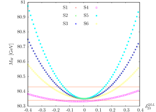
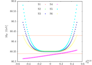
Figure 3: $M_{W}$ as a function of $\delta^{QLL}_{23}$ (upper left), $\delta^{ULR}_{23}$ (upper right) and $\delta^{DLR}_{23}$ (lower).

		Total allowed intervals
$\delta^{QLL}_{23}$	S1 S2 S3 S4 S5 S6	(-0.27:0.28) (-0.23:0.23) (-0.12:0.06) (0.17:0.19) excluded (-0.83:-0.78) (-0.14:0.14) (-0.076:0.14)
$\delta^{ULR}_{23}$	S1 S2 S3 S4 S5 S6	(-0.27:0.27) (-0.27:0.27) (-0.27:0.27) excluded (-0.22:0.22) (-0.37:0.37)
$\delta^{DLR}_{23}$	S1 S2 S3 S4 S5 S6	(-0.0069:0.014) (0.12:0.13) (-0.0069:0.014) (0.11:0.13) (-0.0069:0.014) (0.11:0.13) (0.076:0.12) (0.26:0.30) (-0.014:0.021) (0.17:0.19) (0:0.0069) (0.069:0.076)
$\delta^{URL}_{23}$	S1 S2 S3 S4 S5 S6	(-0.27:0.27) (-0.27:0.27) (-0.27:0.27) excluded (-0.22:0.22) (-0.37:0.37)
$\delta^{DRL}_{23}$	S1 S2 S3 S4 S5 S6	(-0.034:0.034) (-0.034:0.034) (-0.034:0.034) excluded (-0.062:0.062) (-0.021:0.021)
$\delta^{URR}_{23}$	S1 S2 S3 S4 S5 S6	(-0.99:0.99) (-0.99:0.99) (-0.98:0.97) excluded (-0.99:0.99) (-0.96:0.94)
$\delta^{DRR}_{23}$	S1 S2 S3 S4 S5 S6	(-0.96:0.96) (-0.96:0.96) (-0.96:0.94) excluded (-0.97:0.97) (-0.97:-0.94) (-0.63:0.64) (0.93:0.97)

Table 3: Present allowed (by BPO) intervals for the squark mixing parameters $\delta^{FAB}_{ij}$ for the selected S1-S6 MSSM points defined in Tab. 2[14].

		Total allowed intervals
$\delta^{QLL}_{23}$	S1 S2 S3 S4 S5 S6	(-0.18:0.18) (-0.18:0.18) (-0.18:0.18) (-0.53:-0.17)(0.10:0.45) (-0.14:0.14) (-0.23:0.23)
$\delta^{ULR}_{23},\delta^{URL}_{23}$	S1 S2 S3 S4 S5 S6	(-0.41:0.41) (-0.41:0.41) (-0.41:0.41) (0.10:0.50) (-0.39:0.39) (-0.47:0.47)
$\delta^{DLR}_{23},\delta^{DRL}_{23}$	S1 S2 S3 S4 S5 S6	(-0.43:0.43) (-0.43:0.43) (-0.43:0.43) (0.16:0.99) (-0.39:0.39) (-0.49:0.49)

Table 4: Present allowed (by $M_{W}$) intervals for the squark mixing parameters $\delta^{FAB}_{ij}$ for the selected S1-S6 MSSM points defined in Tab. 2.

4.1.3 ${\rm BR}(h\to\bar{b}s+b\bar{s})$

In order to illustrate the contributions from different diagrams we show in Fig. 4 the SUSY-EW, SUSY-QCD and total SUSY contribution to $\Gamma(h\to\bar{b}s+b\bar{s})$ as a function of $\delta^{QLL}_{23}$ (upper left), $\delta^{DLR}_{23}$ (upper right), $\delta^{DRL}_{23}$ (lower left) and $\delta^{DRR}_{23}$ (lower right). These four $\delta^{FAB}_{ij}$ are the only relevant ones, since we are mainly concerned with the down-type sector, and mixing with the first generation does not play a role.

In order to compare our results with the literature, we have used the same set of input parameters as in [9]:

$$\mu =800\,\,\mathrm{GeV},\;m_{\rm SUSY}=800\,\,\mathrm{GeV},\;A_{f}=500\,\,\mathrm{GeV},$$

$$M_{A} =400\,\,\mathrm{GeV},\;M_{2}=300\,\,\mathrm{GeV},\;\tan\beta=35\,,$$ (24)

where we have chosen, for simplicity, $m_{\rm SUSY}$ as a common value for the soft SUSY-breaking squark mass parameters, $m_{\rm SUSY}=M_{\tilde{Q},q}=M_{\tilde{U},(c,t)}=M_{\tilde{D},(s,b)}$, and all the various trilinear parameters to be universal, $A_{f}=A_{t}=A_{b}=A_{c}=A_{s}$. The value of the $\delta^{FAB}_{ij}$’s are varied from -0.9 to 0.9, and GUT relations are used to calculate $M_{1}$ and $M_{3}$. In Ref. [9], only LL mixing was considered. In this limit we find results in qualitative agreement with Ref. [9]. This analysis has been done just to illustrate the different contributions and we do not take into account any experimental constraints. A detailed analysis for realisitic SUSY scenerios (defined in Tab. 2) constrained by BPO and EWPO can be found below.

As can be seen in Fig. 4, for the decay width $\Gamma(h\to\bar{b}s+b\bar{s})$ the SUSY-QCD contribution is dominant in all the cases. For LL mixing shown in the upper left plot, the SUSY-QCD contribution reaches up to ${\cal O}(10^{-6})$, while the SUSY-EW contribution reach up to ${\cal O}(10^{-7})$, resulting in a total contribution “in between”, due to the negative interference between SUSY-EW and SUSY-QCD contribution. For LR and RL mixing, shown in the upper right and lower left plot, respectively, the SUSY-QCD contribution reach up to the maximum value of ${\cal O}(10^{-2})$, while the SUSY-EW contribution reach only up to ${\cal O}(10^{-7})$. In this case total contriution is almost equal to SUSY-QCD contribution as SUSY-EW contibution (and thus the interference) is relatively neglible. For RR mixing, shown in the lower right plot, the SUSY-EW contribution of ${\cal O}(10^{-10})$ is again neglible compared to SUSY-QCD contribution of ${\cal O}(10^{-7})$.

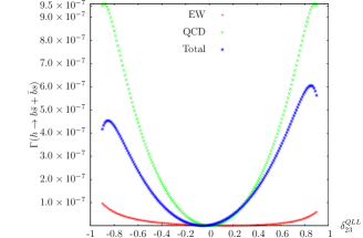
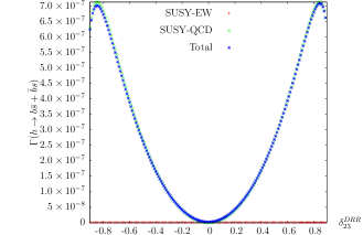
Figure 4: $\Gamma(h\to\bar{b}s+b\bar{s})$ as a function of $\delta^{QLL}_{23}$ (upper left), $\delta^{DLR}_{23}$ (upper right), $\delta^{DRL}_{23}$ (lower left) and $\delta^{DRR}_{23}$ (lower right).

Now we turn to realistic scenarios that are in agreement with experimental data from BPO and EWPO. Starting point are the scenarios S1…S6 defined in Tab. 2, where we vary the flavor violating $\delta^{FAB}_{ij}$ within the experimentally allowed ranges following the results given in Tabs. 3, 4. We start with the scenarios in which we allow one of the $\delta^{FAB}_{ij}$ to be varied, while the others are set to zero. In Fig. 5 we show ${\rm BR}(h\to\bar{b}s+b\bar{s})$as a function of $\delta^{QLL}_{23}$ (upper left), $\delta^{DLR}_{23}$ (upper right), $\delta^{DRL}_{23}$ (lower left) and $\delta^{DRR}_{23}$ (lower right), i.e. for the same set of $\delta^{FAB}_{ij}$ that has been analyzed in Fig. 4. It can be seen that allowing only one $\delta^{FAB}_{ij}\neq 0$ results in rather small values of ${\rm BR}(h\to\bar{b}s+b\bar{s})$. LL (upper left) and RL (lower left plot) mixing results in ${\cal O}(10^{-7})$ values for ${\rm BR}(h\to\bar{b}s+b\bar{s})$. One order of magnitude can be gained in the RR mixing case (lower right). The largest values of ${\rm BR}(h\to\bar{b}s+b\bar{s})$ are obtained in the case of $\delta^{DLR}_{23}\neq 0$ (upper right plot). Here in S4 and S5 values of ${\rm BR}(h\to\bar{b}s+b\bar{s})\sim 2\times 10^{-4}$ can be found, possibly in the reach of future $e^{+}e^{-}$ colliders, see Sect. 3.1.

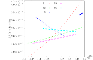
Figure 5: ${\rm BR}(h\to\bar{b}s+b\bar{s})$ as a function of $\delta^{QLL}_{23}$ (upper left), $\delta^{DLR}_{23}$ (upper right), $\delta^{DRL}_{23}$ (lower left) and $\delta^{DRR}_{23}$ (lower right).

So far we have shown the effects of independent variations of one $\delta^{FAB}_{ij}$. Obviously, a realistic model would include several $\delta^{FAB}_{ij}\neq 0$ that may interfere, increasing or decreasing the results obtained with just the addition of independent contributions. GUT based MFV models that induce the flavor violation via RGE running automatically generate several $\delta^{FAB}_{ij}\neq 0$ at the EW scale. In the following we will present results with two or three $\delta^{FAB}_{ij}\neq 0$, where we combined the ones that showed the largest effects.

In Figs. 6-9, in the left columns we show the $3\,\sigma$ contours (with experimental and theory uncertainties added linearly) of ${\rm BR}(B\to X_{s}\gamma)$ (Black), ${\rm BR}(B_{s}\to\mu^{+}\mu^{-})$ (Green), $\Delta M_{B_{s}}$ (Blue) and $M_{W}$ (Red). For non-visible contours the whole plane is allowed by that constraint. The right columns show, for the same parameters, the results for ${\rm BR}(h\to\bar{b}s+b\bar{s})$. In Figs. 6 and 7 we present the results for the plane ($\delta^{QLL}_{23}$, $\delta^{DLR}_{23}$) for S1…S3 and for S4…S6, respectively. Similarly, in Figs. 8 and 9 we show the ($\delta^{DRR}_{23}$, $\delta^{DLR}_{23}$) plane. The shaded area in the left columns indicates the area that is allowed by all experimental constraints. In the ($\delta^{QLL}_{23}$, $\delta^{DLR}_{23}$) planes one can see that the large values for $\delta^{QLL}_{23}$ are not allowed by $M_{W}$, on the other hand, ${\rm BR}(B\to X_{s}\gamma)$ mostly restricts the value of $\delta^{DLR}_{23}$. The largest values for ${\rm BR}(h\to\bar{b}s+b\bar{s})$ in each plane in the arrea allowed by the BPO and the EWPO are summarized in the upper part of Tab. 5. One can see that in most cases we find ${\rm BR}(h\to\bar{b}s+b\bar{s})\sim{\cal O}(10^{-5})$, which would render the observation difficult at current and future colliders. However, in the ($\delta^{QLL}_{23},\delta^{DLR}_{23}$) plane in the scenarios S4 and S5 maximum values of ${\cal O}(3\times 10^{-4})$ can be observed, which could be detectable at future ILC measurements. In the ($\delta^{DRR}_{23}$, $\delta^{DLR}_{23}$) plane for these two scenarios even values of ${\cal O}(10^{-3})$ are reached, which would make a measurement of the flavor violating Higgs decay relatively easy at the ILC.

Plane	MSSM point	Maximum possible value	Figure
($\delta^{QLL}_{23},\delta^{DLR}_{23}$)	S1 S2 S3 S4 S5 S6	$1.38\times 10^{-5}$ $1.39\times 10^{-5}$ $1.43\times 10^{-5}$ $3.34\times 10^{-4}$ $2.74\times 10^{-4}$ $1.36\times 10^{-8}$	Fig. 6 Fig. 6 Fig. 6 Fig. 7 Fig. 7 Fig. 7
($\delta^{DRR}_{23},\delta^{DLR}_{23}$)	S1 S2 S3 S4 S5 S6	$4.41\times 10^{-6}$ $3.32\times 10^{-6}$ $3.07\times 10^{-5}$ $1.66\times 10^{-3}$ $1.97\times 10^{-3}$ $6.03\times 10^{-8}$	Fig. 8 Fig. 8 Fig. 8 Fig. 9 Fig. 9 Fig. 9
($\delta^{QLL}_{23},\delta^{DLR}_{23}$) with $\delta^{DRR}_{23}=0.5$	S1 S2 S3 S4 S5 S6	$7.49\times 10^{-6}$ $7.33\times 10^{-6}$ $3.50\times 10^{-6}$ Excluded Excluded Excluded	Fig. 10 Fig. 10 Fig. 10 Fig. 11 Fig. 11 Fig. 11

Table 5: Maximum possible value for ${\rm BR}(h\to\bar{b}s+b\bar{s})$ for two and three $\delta^{FAB}_{ij}\neq 0$ case for the selected S1-S6 MSSM points defined in Tab. 2.

Figure 6: Left: Contours of ${\rm BR}(B\to X_{s}\gamma)$ (Black), ${\rm BR}(B_{s}\to\mu^{+}\mu^{-})$ (Green), $\Delta M_{B_{s}}$(Blue) and $M_{W}$ (Red) in ($\delta^{QLL}_{23}$ , $\delta^{DLR}_{23}$) plane for points S1-S3. The shaded area shows the range of values allowed by all cronstraints. Right: corresponding countours for ${\rm BR}(h\to\bar{b}s+b\bar{s})$.

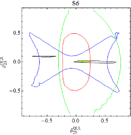
Figure 7: Left: Contours of ${\rm BR}(B\to X_{s}\gamma)$ (Black), ${\rm BR}(B_{s}\to\mu^{+}\mu^{-})$ (Green), $\Delta M_{B_{s}}$ (Blue) and $M_{W}$ (Red) in ($\delta^{QLL}_{23}$ , $\delta^{DLR}_{23}$) plane for points S4-S6. The shaded area shows the range of values allowed by all cronstraints. Right: corresponding countours for ${\rm BR}(h\to\bar{b}s+b\bar{s})$.

Figure 8: Left: Contours of ${\rm BR}(B\to X_{s}\gamma)$ (Black), ${\rm BR}(B_{s}\to\mu^{+}\mu^{-})$ (Green), $\Delta M_{B_{s}}$ (Blue) and $M_{W}$ (Red) in ($\delta^{DRR}_{23}$ , $\delta^{DLR}_{23}$) plane for points S1-S3. The shaded area shows the range of values allowed by all cronstraints. Right: corresponding countours for ${\rm BR}(h\to\bar{b}s+b\bar{s})$.

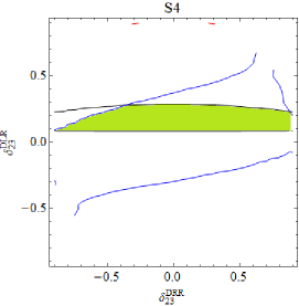
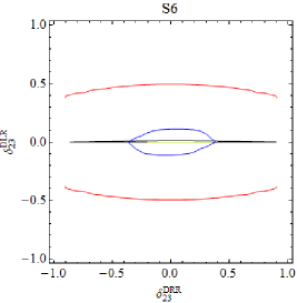
Figure 9: Left: Contours of ${\rm BR}(B\to X_{s}\gamma)$ (Black), ${\rm BR}(B_{s}\to\mu^{+}\mu^{-})$ (Green), $\Delta M_{B_{s}}$ (Blue) and $M_{W}$ (Red) in ($\delta^{DRR}_{23}$ , $\delta^{DLR}_{23}$) plane for points S4-S6. The shaded area shows the range of values allowed by all cronstraints. Right: corresponding countours for ${\rm BR}(h\to\bar{b}s+b\bar{s})$.

As a last step in model independent analysis, we consider the case of three $\delta^{FAB}_{ij}\neq 0$ at a time. For this purpose we scan the parameters in the ($\delta^{QLL}_{23}$, $\delta^{DLR}_{23}$) plane and set $\delta^{DRR}_{23}=0.5$. For reasons of practicability we choose one intermediate value for $\delta^{DRR}_{23}$; a very small value will have no additional effect, and a very large value of $\delta^{DRR}_{23}$ leads to large excluded areas in the ($\delta^{QLL}_{23}$, $\delta^{DLR}_{23}$) plane. We show our results in Figs. 10 and 11 in the scenarios S1-S3 and S4-S6, respectively. Colors and shadings are chosen as in the previous analysis. Here it should be noted that in S4 the whole plane is excluded by $M_{W}$, and in S5 by ${\rm BR}(B_{s}\to\mu^{+}\mu^{-})$ (both contours are not visible). In S6 no overlap between the four constraints is found, and again this scenario is excluded. We have checked that also a smaller value of $\delta^{DRR}_{23}=0.2$ does not qualitatively change the picture for S4, S5 and S6. The highest values that can be reached for ${\rm BR}(h\to\bar{b}s+b\bar{s})$ in the three remaining scenarios in the experimentally allowed regions are shown in the lower part of Tab. 5. One can see only very small valus or ${\cal O}(5\times 10^{-6})$ are found, i.e. choosing $\delta^{DRR}_{23}\neq 0$ did not lead to observable values of ${\rm BR}(h\to\bar{b}s+b\bar{s})$.

To summarize, in our model independent analysis, allowing for more than one $\delta^{FAB}_{ij}\neq 0$ we find that the additional freedom resulted in somewhat larger values of ${\rm BR}(h\to\bar{b}s+b\bar{s})$ as compared to the case of only one non-zero $\delta^{FAB}_{ij}$. In particular in the two scenarios S4 and S5 values of ${\rm BR}(h\to\bar{b}s+b\bar{s})\sim 10^{-3}-10^{-4}$ can be reached, allowing the detection of the flavor violating Higgs decay at the ILC. The other scenarios always yield values that are presumably too low for current and future colliders.

Figure 10: Left: Contours of ${\rm BR}(B\to X_{s}\gamma)$ (Black), ${\rm BR}(B_{s}\to\mu^{+}\mu^{-})$ (Green), $\Delta M_{B_{s}}$ (Blue) and $M_{W}$ (Red) in the ($\delta^{QLL}_{23}$ , $\delta^{DLR}_{23}$) plane with $\delta^{DRR}_{23}=0.5$ for points S1-S3. The shaded area shows the range of values allowed by all cronstraints. Right: corresponding countours for ${\rm BR}(h\to\bar{b}s+b\bar{s})$.

Figure 11: Left: Contours of ${\rm BR}(B\to X_{s}\gamma)$ (Black), ${\rm BR}(B_{s}\to\mu^{+}\mu^{-})$ (Green), $\Delta M_{B_{s}}$ (Blue) and $M_{W}$ (Red) in the ($\delta^{QLL}_{23}$ , $\delta^{DLR}_{23}$) plane with $\delta^{DRR}_{23}=0.5$ for points S4-S6. The shaded area shows the range of values allowed by all cronstraints. Right: corresponding countours for ${\rm BR}(h\to\bar{b}s+b\bar{s})$.

4.2 Numerical results in MFV CMSSM

In this final step of our numerical analysis we investigate the CMSSM as described in Sect. 2.2. Here the MFV hypothesis is realized by demanding no flavor violation at the GUT scale, and the various flavor violating $\delta^{FAB}_{ij}$ are induced by the RGE running to the EW scale. For this analysis the SUSY spectra have been generated with the code SPheno 3.2.4 [54]. We started with the definition of the (MFV) SLHA file [55] at the GUT scale. In a first step within SPheno, gauge and Yukawa couplings at $M_{Z}$ scale are calculated using tree-level formulas. Fermion masses, the $Z$ boson pole mass, the fine structure constant $\alpha$, the Fermi constant $G_{F}$ and the strong coupling constant $\alpha_{s}(M_{Z})$ are used as input parameters. The gauge and Yukawa couplings, calculated at $M_{Z}$, are then used as input for the one-loop RGE’s to obtain the corresponding values at the GUT scale which is calculated from the requirement that $g_{1}=g_{2}$ (where $g_{1,2}$ denote the gauge couplings of the $U(1)$ and $SU(2)$, respectively). The CMSSM boundary conditions (with the numerical values from the SLHA file) are then applied to the complete set of two-loop RGE’s and are evolved to the EW scale. At this point the SM and SUSY radiative corrections are applied to the gauge and Yukawa couplings, and the two-loop RGE’s are again evolved to GUT scale. After applying the CMSSM boundary conditions again the two-loop RGE’s are run down to EW scale to get SUSY spectrum. This procedure is iterated until the required precision is achieved. The output is given in the form of an SLHA, file which is used as input for FeynHiggs to calculate low energy observables discussed above.

In order to get an overview about the size of the effects in the CMSSM parameter space, the relevant parameters $m_{0}$, $m_{1/2}$ have been scanned as, or in case of $A_{0}$ and $\tan\beta$ have been set to all combinations of

$$m_{0} \;=\;500\,\,\mathrm{GeV}\ldots 5000\,\,\mathrm{GeV}~{},$$

$$m_{1/2} \;=\;1000\,\,\mathrm{GeV}\ldots 3000\,\,\mathrm{GeV}~{},$$

$$A_{0} \;=\;-3000,-2000,-1000,0\,\,\mathrm{GeV}~{},$$

$$\tan\beta \;=\;10,20,35,45~{},$$ (25)

with $\mu>0$.

The results are shown in Fig. 12, where we display the contours of ${\rm BR}(h\to\bar{b}s+b\bar{s})$ in the ($m_{0}$, $m_{1/2}$) plane for $\tan\beta=10$, $A_{0}=0$ (upper left), $\tan\beta=10$, $A_{0}=-3000\,\,\mathrm{GeV}$ (upper right), $\tan\beta=45$, $A_{0}=0$ (lower left) and $\tan\beta=45$, $A_{0}=-3000\,\,\mathrm{GeV}$ (lower right). By comparison with planes for other $\tan\beta$-$A_{0}$ combinations we have varyfied that these four planes constitute a representative example. The allowed parameter space can be deduced by comparing to the results presented in Refs. [15, 56]. While not all the planes are in agreement with current constraints, large parts, in particular for larger values of $m_{0}$ and $m_{1/2}$ are compatible with a combination of direct searches, flavor and electroweak precision observables as well as astrophysical data. Upper bounds on $m_{0}$ at the few TeV level could possibly be set by including the findings of Ref. [15] into a global CMSSM analysis.

In Fig. 12 one can see that for most of parameter space values of ${\cal O}(10^{-7})$ are found for ${\rm BR}(h\to\bar{b}s+b\bar{s})$, i.e. outside the reach of current or future collider experiments. Even for the “most extreme” set of parameters we have analyzed, $\tan\beta=45$ and $A_{0}=-3000\,\,\mathrm{GeV}$, no detectable rate has been found. Turning the argument around, any observation of the decay $h\to\bar{b}s+b\bar{s}$ at the (discussed) future experiments would exclude the CMSSM as a possible model.

Figure 12: Contours of ${\rm BR}(h\rightarrow b\bar{s}+\bar{b}s)$ in the $(m_{0}$, $m_{1/2})$ plane for different values of $\tan\beta$ and $A_{0}$ in the CMSSM.

5 Conclusions

We have investigated the flavor violating Higgs boson decay $h\to\bar{b}s+b\bar{s}$ in the MSSM. This evaluation improves on existing analyses in various ways. We take into account the full set of SUSY QCD and SUSY EW corrections, allowing for LL, RL, LR and RR mixing simultaneously. The parameter space is restricted not only by $B$-physics observables, but also by electroweak precision observables, in particular the mass of the $W$ boson. Here we have shown that $M_{W}$ can yield non-trivial, additional restrictions on the parameter space of the flavor violating $\delta^{FAB}_{ij}$.

From the technical side we have (re-)caculated the decay $h\to\bar{b}s+b\bar{s}$ in the FeynArts and FormCalc setup. The BPO and EWPO constraints have been evalated with the help of (a private version of) FeynHiggs, taking into account the full flavor violating one-loop corrections to $M_{W}$ and to the relevant $B$-physics observables (supplemented with further MSSM higher-order corrections). In the GUT based models the low-energy spectra have been evaluated with the help of Spheno.

The first part of the numerical analysis used a model independent approach. In six representative scenarios, which are allowed by current searches for SUSY particles and heavy Higgs bosons, we have evaluated the allowed parameter space for the various $\delta^{FAB}_{ij}$ by applying BPO and EWPO constraints. Within these allowed ranges we have then evaluated ${\rm BR}(h\to\bar{b}s+b\bar{s})$. In the case of only one $\delta^{FAB}_{ij}\neq 0$ we have found that only relatively large values of $\delta^{DLR}_{23}$ could lead to rates of ${\rm BR}(h\to\bar{b}s+b\bar{s})\sim 10^{-4}$, which could be in the detectable range of future $e^{+}e^{-}$ colliders. Allowing two $\delta^{FAB}_{ij}\neq 0$ simultaneously lead to larger values up to ${\rm BR}(h\to\bar{b}s+b\bar{s})\sim 10^{-3}$, which would make the observation at the ILC relatively easy. Allowing for a third $\delta^{FAB}_{ij}\neq 0$, on the other hand, did not lead to larger values of the flavor violating branching ratio.

In the final step of the numerical analysis we have evaluated ${\rm BR}(h\to\bar{b}s+b\bar{s})$ in the MFV Constrained MSSM. In this model the flavor violation is induced by CKM effects in the RGE running from the GUT to the EW scale. Here we have found that also for the “most extreme” set of parameters we have analyzed, $A_{0}=-3000\,\,\mathrm{GeV}$ and $\tan\beta=45$, only negligible effects can be expected. Turning the argument around, detecting a non-zero value for ${\rm BR}(h\to\bar{b}s+b\bar{s})$ at (the discussed) future experiments would exclude the CMSSM as a viable model.

Acknowledgments

The work of S.H. and M.R. was partially supported by CICYT (grant FPA 2013-40715-P). M.G., S.H. and M.R. were supported by the Spanish MICINN’s Consolider-Ingenio 2010 Programme under grant MultiDark CSD2009-00064. M.E.G.  acknowledges further support from the MICINN project FPA2011-23781 and FPA2014-53631-C2-2-P.

References

- [1] S. Glashow, J. Iliopoulos and L. Maiani, Phys. Rev. D2 (1970) 1285.
-
[2]
H. Nilles,
Phys. Rept. 110 (1984) 1;
H. Haber and G. Kane, Phys. Rept. 117 (1985) 75;
R. Barbieri, Riv. Nuovo Cim. 11 (1988) 1. - [3] Y. Amhis et al. [Heavy Flavor Averaging Group], arXiv:1412.7515v1 [hep-ex]
-
[4]
R. Chivukula and H. Georgi,
Phys. Lett. B 188 (1987) 99;
L. Hall and L. Randall, Phys. Rev. Lett. 65 (1990) 2939;
A. Buras et al., Phys. Lett. B 500 (2001) 161. - [5] G. D’Ambrosio et al., Nucl. Phys. B 645 (2002) 155.
- [6] S. Bejar, F. Dilme, J. Guasch and J. Sola, JHEP 0408 (2004) 018 [arXiv:hep-ph/0402188].
- [7] A. Curiel, M. Herrero and D. Temes, Phys. Rev. D 67 (2003) 075008 [arXiv:hep-ph/0210335].
- [8] D. Demir, Phys. Lett. B 571 (2003) 193 [arXiv:hep-ph/0303249].
- [9] A. Curiel, M. Herrero, W. Hollik, F. Merz and S. Peñaranda, Phys. Rev. D 69 (2004) 075009 [arXiv:hep-ph/0312135].
- [10] G. Barenboim, C. Bosch, J. Lee, M. López-Ibáñez and O. Vives, arXiv:1507.08304 [hep-ph].
- [11] M. Gómez, T. Hahn, S. Heinemeyer, M. Rehman, Phys. Rev. D 90 (2014) 074016 [arXiv:1408.0663 [hep-ph]]
- [12] M. Arana-Catania, S. Heinemeyer and M. Herrero, Phys. Rev. D 88 (2013) 1, 015026 [arXiv:1304.2783 [hep-ph]].
- [13] M. Arana-Catania, S. Heinemeyer, M. Herrero and S. Peñaranda, JHEP 1205 (2012) 015 [arXiv:1109.6232 [hep-ph]]; arXiv:1201.6345 [hep-ph].
- [14] M. Arana-Catania, S. Heinemeyer and M. Herrero, Phys. Rev. D 90 (2014) 075003 [arXiv:1405.6960 [hep-ph]].
- [15] M. Gómez, S. Heinemeyer and M. Rehman, Eur. Phys. J. C (2015) 9, 434 [arXiv:1501.02258 [hep-ph]].
- [16] T. Ibrahim and P. Nath, Rev. Mod. Phys. 80 (2008) 577 [arXiv:0705.2008 [hep-ph]].
- [17] M. Pospelov and A. Ritz, Annals Phys. 318 (2005) 119 [arXvi:hep-ph/0504231].
- [18] N. Falck, Z. Phys. C 30 (1986) 247.
- [19] S. Bertolini, F. Borzumati, A. Masiero, and G. Ridolfi, Nucl. Phys. B 353 (1991) 591.
-
[20]
J. Küblbeck, M. Böhm and A. Denner,
Comput. Phys. Commun. 60 (1990) 165;
T. Hahn, Comput. Phys. Commun. 140 (2001) 418 [arXiv:hep-ph/0012260]. -
[21]
T. Hahn and C. Schappacher,
Comput. Phys. Commun. 143 (2002) 54
[arXiv:hep-ph/0105349].
The program and the user’s guide are available via www.feynarts.de . - [22] T. Hahn and M. Pérez-Victoria, Comput. Phys. Commun. 118 (1999) 153 [arXiv:hep-ph/9807565].
-
[23]
S. Heinemeyer, W. Hollik and G. Weiglein,
Comput. Phys. Commun. 124 (2000) 76
[arXiv:hep-ph/9812320];
T. Hahn, S. Heinemeyer, W. Hollik, H. Rzehak and G. Weiglein, Comput. Phys. Commun. 180 (2009) 1426; see www.feynhiggs.de . - [24] S. Heinemeyer, W. Hollik and G. Weiglein, Eur. Phys. J. C 9 (1999) 343 [arXiv:hep-ph/9812472].
- [25] G. Degrassi, S. Heinemeyer, W. Hollik, P. Slavich and G. Weiglein, Eur. Phys. J. C 28 (2003) 133 [arXiv:hep-ph/0212020].
- [26] M. Frank, T. Hahn, S. Heinemeyer, W. Hollik, R. Rzehak and G. Weiglein, JHEP 0702 (2007) 047 [arXiv:hep-ph/0611326].
- [27] T. Hahn, S. Heinemeyer, W. Hollik, H. Rzehak and G. Weiglein, Phys. Rev. Lett. 112 (2014) 14, 141801 [arXiv:1312.4937 [hep-ph]].
- [28] G. Moortgat-Pick et al., Eur. Phys. J. C 75 (2015) 8, 371 [arXiv:1504.01726 [hep-ph]].
- [29] G. Isidori and A. Retico, JHEP 0209 (2002) 063 [arXiv:hep-ph/0208159].
- [30] P. Chankowski and L. Slawianowska, Phys. Rev. D 63 (2001) 054012 [arXiv:hep-ph/0008046].
- [31] J. Foster, K. Okumura and L. Roszkowski, JHEP 0508 (2005) 094 [arXiv:hep-ph/0506146].
-
[32]
G. Isidori and P. Paradisi,
Phys. Lett. B 639 (2006) 499
[arXiv:hep-ph/0605012];
G. Isidori, F. Mescia, P. Paradisi and D. Temes, Phys. Rev. D 75 (2007) 115019 [arXiv:hep-ph/0703035], and references therein. -
[33]
See: https://www.slac.stanford.edu/xorg/hfag/rare/2013/radll/
OUTPUT/TABLES/radll.pdf . - [34] M. Misiak, Acta Phys. Polon. B 40 (2009) 2987 [arXiv:0911.1651 [hep-ph]].
- [35] S. Chatrchyan et al. [CMS Collaboration], Phys. Rev. Lett. 111 (2013) 101804 [arXiv:1307.5025 [hep-ex]].
- [36] R. Aaij et al. [LHCb Collaboration], Phys. Rev. Lett. 111 (2013) 101805 [arXiv:1307.5024 [hep-ex]].
- [37] A. Buras, J. Girrbach, D. Guadagnoli and G. Isidori, Eur. Phys. J. C 72 (2012) 2172 [arXiv:1208.0934 [hep-ph]].
- [38] See: https://www.slac.stanford.edu/xorg/hfag/osc/PDG_2013/ .
- [39] A. Buras, M. Jamin and P. Weisz, Nucl. Phys. B 347 (1990) 491.
- [40] E. Golowich, J. Hewett, S. Pakvasa, A. Petrov and G. Yeghiyan, Phys. Rev. D 83 (2011) 114017 [arXiv:1102.0009 [hep-ph]].
- [41] CMS and LHCb Collaborations, CMS-PAS-BPH-13-007, LHCb-CONF-2013-012, CERN-LHCb-CONF-2013-012.
- [42] S. Heinemeyer, W. Hollik and G. Weiglein, Phys. Rept. 425 (2006) 265 [arXiv:hep-ph/0412214].
-
[43]
S. Schael et al. [ALEPH and DELPHI and L3 and OPAL and LEP
Electroweak Collaborations],
Phys. Rept. 532 (2013) 119
[arXiv:1302.3415 [hep-ex]];
see http://www.cern.ch/LEPEWWG . -
[44]
M. Baak et al., arXiv:1310.6708 [hep-ph];
A. Freitas et al., arXiv:1307.3962 [hep-ph]. -
[45]
S. Heinemeyer,
talk given at the 8th FCC-ee Physics Workshop,
Paris, France, October 2014, see:
https://indico.cern.ch/event/337673/session/3/contribution/
41/material/slides . - [46] M. Veltman, Nucl. Phys. B 123 (1977) 89.
- [47] S. Heinemeyer, W. Hollik, F. Merz and S. Peñaranda, Eur. Phys. J. C 37 (2004) 481 [arXiv:hep-ph/0403228].
- [48] A. Djouadi, P. Gambino, S. Heinemeyer, W. Hollik, C. Jünger and G. Weiglein, Phys. Rev. Lett. 78 (1997) 3626 [arXiv:hep-ph/9612363]; Phys. Rev. D 57 (1998) 4179 [arXiv:hep-ph/9710438].
- [49] S. Heinemeyer, W. Hollik, D. Stöckinger, A. Weber, and G. Weiglein JHEP 08 (2006) 052 [arXiv:hep-ph/0604147]
- [50] J. Haestier, S. Heinemeyer, D. Stöckinger and G. Weiglein JHEP 0512 (2005) 027 [arXiv:hep-ph/0508139]
- [51] H. Haber and Y. Nir, Nucl. Phys. B 335 (1990) 363.
-
[52]
M. Dührssen, talk given at ‘Rencontres de Moriond EW 2015”, see:
https://indico.in2p3.fr/event/10819/session/3/contribution/102/material/
slides/1.pdf . -
[53]
P. Bechtle, O. Brein, S. Heinemeyer, G. Weiglein
and K. Williams,
Comput. Phys. Commun. 181 (2010) 138
[arXiv:0811.4169 [hep-ph]];
Comput. Phys. Commun. 182 (2011) 2605
[arXiv:1102.1898 [hep-ph]];
P. Bechtle, O. Brein, S. Heinemeyer, O. Stål, T. Stefaniak, G. Weiglein and K. Williams, Eur. Phys. J. C 74 (2014) 2693 [arXiv:1311.0055 [hep-ph]]. -
[54]
W. Porod,
Comput. Phys. Commun. 153 (2003) 275
[arXiv:hep-ph/0301101];
W. Porod and F. Staub, Comput. Phys. Commun. 183 (2012) 2458 [arXiv:1104.1573 [hep-ph]]. -
[55]
P. Skands et al.,
JHEP 0407 (2004) 036
[arXiv:hep-ph/0311123];
B. Allanach et al., Comput. Phys. Commun. 180 (2009) 8 [arXiv:0801.0045 [hep-ph]]. - [56] O. Buchmueller et al., Eur. Phys. J. C 74 (2014) 6, 2922 [arXiv:1312.5250 [hep-ph]]; arXiv:1508.01173 [hep-ph].