Universality in survivor distributions:
Characterising the winners of competitive dynamics

Abstract

We investigate the survivor distributions of a spatially extended model of competitive dynamics in different geometries. The model consists of a deterministic dynamical system of individual agents at specified nodes, which might or might not survive the predatory dynamics: all stochasticity is brought in by the initial state. Every such initial state leads to a unique and extended pattern of survivors and non-survivors, which is known as an attractor of the dynamics. We show that the number of such attractors grows exponentially with system size, so that their exact characterisation is limited to only very small systems. Given this, we construct an analytical approach based on inhomogeneous mean-field theory to calculate survival probabilities for arbitrary networks. This powerful (albeit approximate) approach shows how universality arises in survivor distributions via a key concept – the dynamical fugacity. Remarkably, in the large-mass limit, the survival probability of a node becomes independent of network geometry, and assumes a simple form which depends only on its mass and degree.

I Introduction

The fate of agents in any situation where death is a possibility attracts enormous interest: here, death does not have to be literal, but could also refer to bankruptcies in a financial context or oblivion in the context of ideas. This panorama of situations is usually captured by agent-based models including predator-prey models, the best known being the Lotka-Volterra model Murray (1989); Berryman (1992); Szabó and Fáth (2007) or indeed, winner-takes-all models, which embody the survival of the largest, or the fittest. The model we study here belongs to the second category; the most massive agents grow at the cost of their smaller neighbors, which eventually disappear. Motivated by the physics of interacting black holes in brane-world cosmology Majumdar (2003); Majumdar et al. (2005), its behavior in mean-field and on different lattices was investigated at length in Luck and Mehta (2005), followed by simulations on more complex geometries Thyagu and Mehta (2011); Aich and Mehta (2014). The essence of the model in its original context Majumdar (2003); Majumdar et al. (2005) involved the competition between black holes of different masses, in the presence of a universal dissipative ‘fluid’. The model also turned out to have a ‘rich-get-richer’ interpretation in the context of economics, where it was related to the survival dynamics of competing traders in a marketplace in the presence of taxation (dissipation) Mehta (2013); Mehta et al. (2005).

One of the most important questions to be asked of such models concerns the distribution of survivors, i.e., those agents who survive the predatory dynamics. In spatially extended models, the presence of multiple interactions makes this a difficult question to answer in full generality. The seemingly universal distributions of survivor patterns put forward in Thyagu and Mehta (2011) motivated us to ask: can one provide a theoretical framework for the appearance of some universal features in survivor distributions? The answer is yes, as we will demonstrate in this paper.

We first introduce a much simpler version of the model investigated earlier Luck and Mehta (2005); Thyagu and Mehta (2011); Mehta (2013); Aich and Mehta (2014), which, however, preserves features such as the exponential multiplicity of attractors (Section II) essential to its complexity. We characterize exactly the attractors reached by the dynamics on chains and rings of increasing sizes (Section III), an exercise which illustrates how a very intrinsic complexity makes such computations rapidly impossible. This leads us to formulate an approximate analytical treatment of the problem on random graphs and networks (Section IV), based on inhomogeneous mean-field theory, which yields rather accurate predictions for the survival probability of a node, given its degree and/or its initial mass.

II The model

The degrees of freedom of the present model consist of a time-dependent positive mass $y_{i}(t)$ at each node $i$ of a graph. These masses are subject to the following first-order dynamics:

$$\frac{{\rm d}y_{i}}{{\rm d}t}=\left(1-g\sum_{j(i)}y_{j}\right)y_{i}.$$ (1)

Each node $i$ is symmetrically (i.e., non-directionally) coupled to its neighbors, which are all nodes $j$ connected to $i$ by a bond; $g$ is a positive coupling constant.

The dynamics are deterministic, so that all stochasticity comes from the distribution of initial masses $y_{i}(0)$. This model is a much simpler version of the one investigated in Luck and Mehta (2005) which was inspired by black-hole physics Majumdar (2003); Majumdar et al. (2005). In particular the explicit time dependence and initial big-bang singularity of that model are here dispensed with; only a simple nonlinearity, quadratic in the masses, is retained. Despite these simplifications, the present model keeps the most interesting features of its predecessor, such as those to do with its multiplicity of attractors.

The coupling constant $g$ can be scaled out by means of a linear rescaling of the masses:

$$z_{i}(t)=gy_{i}(t).$$ (2)

The new dynamical variables indeed obey

$$\frac{{\rm d}z_{i}}{{\rm d}t}=\left(1-\sum_{j(i)}z_{j}\right)z_{i}.$$ (3)

As a matter of fact, the model has a deeper dynamical symmetry. Setting

$$y_{i}(t)=a_{i}(\tau)\,{\rm e}^{t},$$ (4)

where $\tau$ is a global proper time, so that ${\rm d}\tau=g\,{\rm e}^{t}\,{\rm d}t$, i.e.,

$$\tau=g({\rm e}^{t}-1),$$ (5)

the dynamical equations (1) can be recast as

$$\frac{{\rm d}a_{i}}{{\rm d}\tau}=-\left(\sum_{j(i)}a_{j}\right)a_{i}.$$ (6)

Remarkably, the dynamics so defined are entirely parameter-free. Quadratic differential systems such as the above have attracted much attention in the mathematical literature, such as in discussions of Hilbert’s 16th problem (see e.g. Jenks (1969); Li (2003)).

Equations (6) can be formally integrated as

$$a_{i}(\tau)=a_{i}(0)\,\exp\left(-\int_{0}^{\tau}\sum_{j(i)}a_{j}(\tau^{\prime})\,{\rm d}\tau^{\prime}\right).$$ (7)

The amplitudes $a_{i}(\tau)$ are therefore decreasing functions of $\tau$. For each node $i$, either of two things might happen:

• Node $i$ survives asymptotically. This occurs when the integral in (7) converges in the $\tau\to\infty$ limit. The amplitude $a_{i}(\tau)$ reaches a non-zero limit $a_{i}(\infty)$, so that the mass $y_{i}(t)$ grows exponentially as

  $$y_{i}(t)\approx a_{i}(\infty){\rm e}^{t}.$$ (8)

• Node $i$ does not survive asymptotically. This occurs when the integral in (7) diverges in the $\tau\to\infty$ limit. This divergence is generically linear, so that the amplitude $a_{i}(\tau)$ falls off to zero exponentially fast in $\tau$, while the mass $y_{i}(t)$ falls off as a double exponential in time $t$.

The dynamics therefore drive the system to a non-trivial attractor, i.e., an extended pattern of survivors and non-survivors. This attractor depends on the whole initial mass profile (although it is independent of the overall mass scale). The formula (7) generically implies the following local constraints:

1. each survivor is isolated (all its neighbors are non-survivors),

2. each non-survivor has at least one survivor among its neighbors.

Conversely, every pattern obeying the above constraints is realized as an attractor of the dynamics, for some domain of initial data. This situation is therefore similar to that met in a variety of statistical-mechanical models ranging from glasses to systems with kinetic constraints. Attractors play the role of metastable states, which have been given various names, such as valleys, pure states, quasi-states or inherent structures Thouless et al. (1977); Kirkpatrick and Sherrington (1978); Stillinger and Weber (1982); Kirkpatrick and Wolynes (1987); Franz and Virasoro (2000). In all these situations the number $M$ of metastable states grows exponentially with system size $N$ as

$$M\sim{\rm e}^{N\Sigma},$$ (9)

where $\Sigma$ is the configurational entropy or complexity. This quantity is not known exactly in general, except in the one-dimensional case where it can be determined by means of a transfer-matrix approach (see Appendix A). It is relevant to mention the Edwards ensemble here, which is constructed by assigning a thermodynamical significance to the configurational entropy Edwards (1994). According to the Edwards hypothesis, all the attractors of a given ensemble (e.g. at fixed survivor density) are equally probable. This hypothesis holds generically for mean-field models, while it is weakly violated for finite-dimensional systems Franz and Virasoro (2000); Dean and Lefèvre (2001); Berg and Mehta (2001); Prados and Brey (2001); de Smedt et al. (2002); Godrèche and Luck (2005).

III Exact results for small systems

In this section we consider the model on small one-dimensional graphs, i.e., closed rings and open chains of $N$ nodes. In one dimension, (1) and (6) read

$$\frac{{\rm d}y_{n}}{{\rm d}t} = \left(1-g(y_{n-1}+y_{n+1})\right)y_{n},$$ (10)

$$\frac{{\rm d}a_{n}}{{\rm d}\tau} = -(a_{n-1}+a_{n+1})a_{n},$$ (11)

for $n=1,\dots,N$, with appropriate boundary conditions: periodic ($a_{0}=a_{N}$, $a_{N+1}=a_{1}$) for rings and Dirichlet ($a_{0}=a_{N+1}=0$) for chains.

Equations (11) are very reminiscent of those defining the integrable Volterra chain. The coupling term involves the sum $a_{n-1}+a_{n+1}$ in the present model, whereas it involves the difference $a_{n-1}-a_{n+1}$ in the Volterra system. The appearance of a difference is however essential for integrability Mikhailov et al. (1987); Yamilov (2006). The present model is therefore not integrable, even in one dimension.

Our goal is to characterize the attractor reached by the dynamics on small systems of increasing sizes, as a function of the initial mass profile. This task soon becomes intractable, except on very small systems, due to the intrinsic complexity of the model. The numbers $M_{N}^{({\rm r})}$ and $M_{N}^{({\rm c})}$ of these attractors on rings and chains of $N$ nodes are given in Table 2 of Appendix A. These numbers grow exponentially fast with $N$, according to (9), with $\Sigma$ given by (86).

Ring with $N=2$

The system consists of two nodes connected by two bonds. Both attractors consist of a single survivor. The dynamical equations (11) read

$$\frac{{\rm d}a_{1}}{{\rm d}\tau}=\frac{{\rm d}a_{2}}{{\rm d}\tau}=-2a_{1}a_{2}.$$ (12)

The difference $D=a_{1}-a_{2}$ is a conserved quantity. If $a_{1}(0)>a_{2}(0)$, the attractor is $\langle 1\rangle$ (meaning that only node 1 survives) and its final amplitude is

$$a_{1}(\infty)=D=a_{1}(0)-a_{2}(0),$$ (13)

and vice versa. The survivor is always the node with the larger initial mass.

In the borderline case of equal initial masses, the integrals in (7) are marginally (logarithmically) divergent. Both masses saturate to the universal limit $y_{1}(\infty)=y_{2}(\infty)=1/(2g)$, irrespective of their initial value.

Chain with $N=2$

The two nodes are now connected by a single bond. The dynamical equations are identical to (12), up to an overall factor of two. Here too, the more massive node is the survivor.

Ring with $N=3$

The attractors again consist of a single survivor. Although there is no obviously conserved quantity, the attractor can be predicted by noticing that

$$\frac{{\rm d}}{{\rm d}\tau}(a_{2}-a_{1})=-(a_{2}-a_{1})a_{3}.$$ (14)

The sign of any difference $a_{i}-a_{j}$ is therefore conserved by the dynamics. In other words, the order of the masses is conserved. In particular the survivor is the node with the largest initial mass.

Chain with $N=3$

The central node 2 plays a special role, so that the two attractors are $\langle 2\rangle$ and $\langle 13\rangle$. There are two conserved quantities, $D=a_{1}-a_{2}+a_{3}$ and $R=a_{1}/a_{3}$. If $D>0$, the attractor is $\langle 13\rangle$ and the final amplitudes read

$$\frac{a_{1}(\infty)}{a_{1}(0)}=\frac{a_{3}(\infty)}{a_{3}(0)}=\frac{D}{a_{1}(0)+a_{3}(0)}.$$ (15)

If $D<0$, the attractor is $\langle 2\rangle$ and $a_{2}(\infty)=|D|$.

Ring with $N=4$

The two attractors are the ‘diameters’ $\langle 13\rangle$ and $\langle 24\rangle$. The alternating sum $D=a_{1}-a_{2}+a_{3}-a_{4}$ is a conserved quantity. If $D>0$, the attractor is $\langle 13\rangle$ and $a_{1}(\infty)+a_{3}(\infty)=D$. If $D<0$, the attractor is $\langle 24\rangle$ and $a_{2}(\infty)+a_{4}(\infty)=|D|$. The attractor is therefore always the diameter with the larger total initial mass. The individual asymptotic amplitudes cannot however be determined in general.

Chain with $N=4$

The three attractors are $\langle 13\rangle$, $\langle 14\rangle$ and $\langle 24\rangle$. The alternating sum $D=a_{1}-a_{2}+a_{3}-a_{4}$ is a conserved quantity. This is the first case where the attractor cannot be predicted analytically in general.

Figure 1 shows the attractors reached as a function of $a_{2}(0)$ and $a_{3}(0)$, for fixed $a_{1}(0)=a_{4}(0)=0.3$. It is clear that $\langle 13\rangle$ can only be reached for $D>0$, i.e., above the diagonal, whereas $\langle 24\rangle$ can only be reached for $D<0$, i.e., below the diagonal. The intermediate pattern $\langle 14\rangle$ is observed in a central region near the diagonal. The form of this region can be predicted to some extent. On the horizontal axis, the transition from $\langle 14\rangle$ to $\langle 24\rangle$ takes place for $a_{2}(0)=a_{1}(0)=0.3$. Similarly, on the vertical axis, the transition from $\langle 14\rangle$ to $\langle 13\rangle$ takes place for $a_{3}(0)=a_{4}(0)=0.3$. The central region where $\langle 14\rangle$ is the attractor shrinks rapidly with increasing distance from the origin. This can be explained by considering the dynamics on the diagonal, i.e., in the symmetric situation where $a_{1}(0)=a_{4}(0)$ and $a_{2}(0)=a_{3}(0)$. These symmetries are preserved by the reduced dynamics

$$\frac{{\rm d}a_{1}}{{\rm d}\tau}=-a_{1}a_{2},\quad\frac{{\rm d}a_{2}}{{\rm d}\tau}=-(a_{1}+a_{2})a_{2}.$$ (16)

The reduced attractor is $\langle 1\rangle$, the full attractor is $\langle 14\rangle$, and $D$ vanishes identically. The reduced dynamics have another conserved quantity, $C=a_{1}\exp(-a_{2}/a_{1})$. The asymptotic amplitude $a_{1}(\infty)=C$ becomes exponentially small as $a_{2}(0)$ increases. The width of the central green region is expected to follow the same scaling law, i.e., to become exponentially narrow with distance from the origin, in agreement with our observation.

Figure 1: (Color online) Attractor on the chain with $N=4$ in the $a_{2}(0)$–$a_{3}(0)$ plane, for fixed $a_{1}(0)=a_{4}(0)=0.3$.

Ring with $N=5$

There are five attractors consisting of two survivors, obtained from each other by rotation: $\langle 13\rangle$, $\langle 24\rangle$, $\langle 35\rangle$, $\langle 14\rangle$ and $\langle 25\rangle$. There is no obviously conserved quantity, and the attractor cannot be predicted analytically in general.

Figure 2 shows the attractors as a function of $a_{4}(0)$ and $a_{5}(0)$, for fixed $a_{1}(0)=0.5$, $a_{2}(0)=0.7$ and $a_{3}(0)=0.6$. The five attractors meet at point P $(a_{4}(0)=0.363094,\;a_{5}(0)=0.313748)$. If launched at P, the system is driven to the unique symmetric solution where all masses converge to the universal limit $1/(2g)$. A linear stability analysis around the latter solution reveals that its stable manifold is three-dimensional, in agreement with the observation that its intersection with the plane of the figure is the single point P.

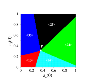
Figure 2: (Color online) Attractor on the ring with $N=5$ in the $a_{4}(0)$–$a_{5}(0)$ plane, for fixed $a_{1}(0)=0.5$, $a_{2}(0)=0.7$ and $a_{3}(0)=0.6$. The five attractors meet at point P.

This is the first case which manifests one of the most interesting features of the model, that of ‘winning against the odds’ Thyagu and Mehta (2011); Mehta (2013); Aich and Mehta (2014). Numerical simulations with two structureless distributions of initial masses, uniform (uni) and exponential (exp), yield the following observations:

• The probability that the node with largest initial mass is a survivor is 0.849 (uni) or 0.937 (exp);

• The probability that the attractor corresponds to the largest initial mass sum among the possible attractors is 0.791 (uni) or 0.891 (exp);

• The probability that the node with smallest initial mass is a survivor is 0.018 (uni) or 0.019 (exp).

This small but non-zero probability for the smallest initial mass to survive is the beginning of the complexity associated with the phenomenon of winning against the odds. It happens essentially because more distant nodes can destroy massive intermediaries between themselves and the small masses concerned, thereby letting the latter survive ‘against the odds’. For larger sizes, the problem soon becomes intractable. First, the number of attractors grows exponentially fast with $N$; second, larger system sizes make for increased interaction ranges for a given node. This makes it increasingly probable to have winners against the odds, making it more and more difficult to predict attractors based only on initial mass distributions.

The above algorithmic complexity goes hand in hand with the violation of the Edwards hypothesis as well as other specific out-of-equilibrium features of the attractors, including a superexponential spatial decay of various correlations Luck and Mehta (2005). This phenomenon, put forward in zero-temperature dynamics of spin chains de Smedt et al. (2002), is reminiscent of the behaviour of a larger class of fully irreversible models, exemplified by random sequential adsorption (RSA) Evans (1993).

IV Approximate analytical treatment

Despite the complexity referred to above, we show here that some ‘one-body observables’ can be predicted by an approximate analytical approach. Our techniques are based on the inhomogeneous mean-field theory and rely on the assumption that the statistical properties of a node only depend on its degree $k$ Pastor-Satorras and Vespignani (2001). Such ideas have been successfully applied to a wide class of problems on complex networks (see Barrat et al. (2008); Pastor-Satorras et al. (2015) for reviews). The thermodynamic limit is implicitly taken; also, the embedding graph is replaced by an uncorrelated random graph whose nodes have probabilities $p_{k}$ to be connected to $k$ neighbors, i.e, to have degree $k$. In this section, we use this framework to evaluate the survival probability of a node, given its degree and/or initial mass.

IV.1 Survival probability of a typical node

We consider first the simplest observable – the survival probability of a typical node, irrespective of initial mass or degree.

From the reduced dynamical equations (6), the initial decay rate of the amplitude $a_{i}(\tau)$ of node $i$ is seen to be:

$$\omega_{i}=\sum_{j(i)}a_{j}(0)=\sum_{j(i)}y_{j}(0).$$ (17)

If node $i$ has degree $k$, the above expression is the sum of the $k$ initial masses of the neighboring nodes.

From a modelling point of view, this suggests a decimation process in continuous time, where nodes are removed at a rate given by their degree $k$ at time $t$. The initial graph is entirely defined by the probabilities $p_{k}$ for a node to have degree $k$. Its subsequent evolution during the decimation process is characterized by its time-dependent degree distribution, i.e., by the fractions $q_{k}(t)$ of initial nodes which still survive at time $t$ and have degree $k$. The latter quantities start from

$$q_{k}(0)=p_{k}$$ (18)

at the beginning of the process ($t=0$) and converge to

$$q_{k}(\infty)=S\,\delta_{k0}$$ (19)

at the end of the process ($t\to\infty$). Indeed, as in the original model, survivors are isolated, so that their final degree is zero. The amplitude $S$ is the quantity of interest, as it represents the survival probability of a typical node. Our goal is to determine it as a function of the probabilities $p_{k}$.

The $q_{k}(t)$ obey the dynamical equations

$$\frac{{\rm d}q_{k}(t)}{{\rm d}t} = -kq_{k}(t)$$ (20)

$$+ \lambda(t)\left((k+1)q_{k+1}(t)-kq_{k}(t)\right).$$

The first line corresponds to the removal of a node of degree $k$ at constant rate $k$, while the second line describes the dynamics of its neighbors. The removal of one neighboring node adds to the fraction $q_{k}(t)$ at a rate proportional to $(k+1)q_{k+1}(t)$ while it depletes it at a rate proportional to $kq_{k}(t)$.

The time-dependent quantity $\lambda(t)$ is the rate at which a random neighbor of a given node is removed at time $t$, which is, consistent with the above, given by the average degree of a random neighbor of the node at time $t$. This rate can be evaluated as follows (see e.g. Pastor-Satorras et al. (2015)). The probability that a node of degree $k$ has a neighbor of degree $\ell$ at time $t$ is, for an uncorrelated network, independent of $k$, and given by $\widetilde{q}_{\ell}(t)=\ell q_{\ell}(t)/\langle\ell(t)\rangle$. (The shift from $q_{\ell}(t)$ to $\widetilde{q}_{\ell}(t)$ is related to the ‘inspection paradox’ in probability theory (see e.g. Feller (1966)).) The average degree of a random neighbor of the node at time $t$ is then given by $\sum_{\ell}\ell\widetilde{q}_{\ell}(t)$, i.e.,

$$\lambda(t)=\frac{\langle k(t)^{2}\rangle}{\langle k(t)\rangle}.$$ (21)

Introducing the generating series

$$P(z)=\sum_{k\geq 0}p_{k}z^{k},\quad Q(z,t)=\sum_{k\geq 0}q_{k}(t)z^{k},$$ (22)

we see that $Q(z,t)$ obeys the partial differential equation

$$\frac{\partial Q}{\partial t}+\left(z+(z-1)\lambda(t)\right)\frac{\partial Q}{\partial z}=0,$$ (23)

with initial condition

$$Q(z,0)=P(z).$$ (24)

Hence it is invariant along the characteristic curves defined by

$$\frac{{\rm d}z}{{\rm d}t}=z+(z-1)\lambda(t).$$ (25)

This differential equation can be integrated as

$$z_{0}=1+(z_{t}-1){\rm e}^{-t-\Lambda(t)}-\int_{0}^{t}{\rm e}^{-s-\Lambda(s)}\,{\rm d}s,$$ (26)

with

$$\Lambda(t)=\int_{0}^{t}\lambda(s)\,{\rm d}s.$$ (27)

We have therefore

$$Q(z_{t},t)=P(z_{0}).$$ (28)

For infinitely long times, irrespective of $z_{t}$, the parameter $z_{0}$ which labels the characteristic curves converges to the limit

$$\zeta=1-\int_{0}^{\infty}{\rm e}^{-t-\Lambda(t)}\,{\rm d}t,$$ (29)

which we call the dynamical fugacity of the model.

We are left with the following simple expression for the survival probability of a typical node (see (19))

$$S=P(\zeta).$$ (30)

Furthermore, the fugacity $\zeta$ can be shown to be implicitly given by

$$2{\langle k\rangle}\int_{\zeta}^{1}\frac{{\rm d}z}{P^{\prime}(z)}=1,$$ (31)

where the accent denotes a derivative.

We list a few quantitative predictions for important graphs/networks below:

• Erdös-Rényi (ER) graph. This historical example of a random graph Erdös and Rényi (1959, 1960) has a Poissonian degree distribution of the form

  $$p_{k}={\rm e}^{-a}\,\frac{a^{k}}{k!}\quad(k\geq 0),$$ (32)

  so that ${\langle k\rangle}=a$ and $P(z)={\rm e}^{a(z-1)}$. We obtain

  $$\zeta=1-\frac{1}{a}\ln\frac{a+2}{2},$$ (33)

  $$S=\frac{2}{a+2}.$$ (34)

• $K$-regular graph. In the case of a $K$-regular graph, where all nodes have the same degree $K\geq 2$, we have $P(z)=z^{K}$. We obtain

  $$\zeta=\left(\frac{2}{K}\right)^{1/(K-2)},$$ (35)

  $$S=\left(\frac{2}{K}\right)^{K/(K-2)}\quad(K\geq 3).$$ (36)

  For $K=2$ the above results become

  $$\zeta={\rm e}^{-1/2}=0.606530,$$ (37)

  $$S={\rm e}^{-1}=0.367879.$$ (38)

• Geometric graph. In the case of a geometric degree distribution with parameter $y$, i.e.,

  $$p_{k}=(1-y)y^{k}\quad(k\geq 0),$$ (39)

  we have ${\langle k\rangle}=y/(1-y)$ and $P(z)=(1-y)/(1-yz)$. We obtain

  $$\zeta = \frac{1}{y}-\left(\frac{(1-y)^{2}(2+y)}{2y^{3}}\right)^{1/3}$$ (40)

  $$= 1+\frac{1}{{\langle k\rangle}}-\left(\frac{3{\langle k\rangle}+2}{2{\langle k\rangle}^{3}}\right)^{1/3},$$

  $$S = \left(\frac{2(1-y)}{2+y}\right)^{1/3}=\left(\frac{2}{3{\langle k\rangle}+2}\right)^{1/3}.$$ (41)

• Barabási-Albert (BA) network. The BA network, grown with a linear law of preferential attachment, has a degree distribution Barabási and Albert (1999); Barabási et al. (1999)

  $$p_{k}=\frac{4}{k(k+1)(k+2)}\quad(k\geq 1)$$ (42)

  with a power-law tail with exponent $\gamma=3$. We have ${\langle k\rangle}=2$ and

  $$P(z)=3-\frac{2}{z}-\frac{2(1-z)^{2}}{z^{2}}\ln(1-z).$$ (43)

  Solving (31) numerically, we obtain

  $$\zeta=0.67016,\quad S=0.55300.$$ (44)

• Generalized preferential attachment (GPA) network. This is a generalization of the BA network, where the attachment probability to an existing node with degree $k$ is proportional to $k+c$ Dorogovtsev et al. (2000); Krapivsky et al. (2000); Godrèche et al. (2009), with the offset $c$ representing the initial attractiveness of a node. The degree distribution

  $$p_{k}=\frac{(c+2)\Gamma(2c+3)\Gamma(k+c)}{\Gamma(c+1)\Gamma(k+2c+3)}\quad(k\geq 1)$$ (45)

  has a power-law tail with a continuously varying exponent $\gamma=c+3$. We have, as expected for a tree, ${\langle k\rangle}=2$, irrespective of $c$, and

  $$P(z) = \frac{c+2}{2c+3}\,z(1-z)^{c+2}$$ (46)

  $$\times {{}_{2}F_{1}}(c+3,2c+3;2c+4;z),$$

  where ${{}_{2}F_{1}}$ is the Gauss hypergeometric function.

  The GPA network can be simulated efficiently by means of a redirection algorithm Krapivsky and Redner (2001, 2002). Every new node is attached either to a uniformly chosen earlier node with probability $1-\nu$, or to the ancestor of the latter node with the redirection probability

  $$\nu=\frac{1}{c+2}.$$ (47)

  For $\nu\to 0$ (i.e., $c\to+\infty$), we have a uniform attachment rule, yielding $p_{k}=2^{-k}$ and $P(z)=z/(2-z)$, so that

  $$\zeta=2-(5/2)^{1/3}=0.642791,$$ (48)

  $$S=2(2/5)^{1/3}-1=0.473612.$$ (49)

  For $\nu\to 1$ (i.e., $c\to-1$), the model becomes singular. The $p_{k}$ converge to $\delta_{k,1}$, while we still have ${\langle k\rangle}=2$, formally. In this singular limit we have

  $$\zeta=S=\frac{3}{4}$$ (50)

  Finally, the BA network is recovered for $\nu=1/2$ (i.e., $c=0$).

Figure 3 provides a summary of the above results. The survival probability $S$ of a typical node is plotted against the mean degree ${\langle k\rangle}$, for all the above. Turning to the specific example of the GPA networks, we note that (48) and (49) provide lower bounds for the dynamical fugacity $\zeta$ and the survival probability $S$ respectively, which both increase to their upper bounds (50) as functions of the redirection probability $\nu$. This trend is reflected in the blue arrowheads in Figure 3, where the blue square corresponds to the value for the BA network.

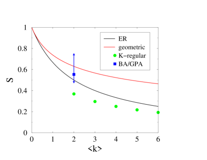
Figure 3: (Color online) Survival probability $S$ of a typical node, as predicted by our approximate analysis, against mean degree ${\langle k\rangle}$ for several examples of graphs and networks. For the ER and geometric graphs, the predictions for continuously varying ${\langle k\rangle}$ are shown as the black (lower) and red (upper) curves. Green filled circles correspond to $K$-regular graphs for integer $K$. The blue square shows the prediction (44) for the BA network, while the vertical bar with arrowheads shows the range of values of $S$ for GPA networks, given by the bounds (49) and (50).

In order to test the above for a few simple cases, we have measured the survival probability $S$ of a typical node in three different geometries: the 1D chain, the 2D square lattice and the BA network. We solved the dynamical equations (6) numerically, with initial masses drawn either from a uniform (uni) or an exponential (exp) distribution. The measured values of $S$ are listed in Table 1, together with our approximate predictions (36), (38) and (44).

Geometry	1D	2D	BA
$S_{\rm uni}$	$\ 0.4393\$	$\ 0.3851\$	$\ 0.6891\$
$S_{\rm exp}$	0.4360	0.3755	0.6767
$S_{\rm pred}$	0.3679	0.2500	0.5530

Table 1: Survival probability of a typical node of the 1D chain, the 2D square lattice and the BA network. Comparison of numerical results for uniform (uni) and exponential (exp) mass distributions and approximate analytical results (pred).

Our numerical results suggest that the survival probability depends only weakly on the mass distribution, as long as the latter is rather structureless. While our predictions are systematically lower than the numerical observations, they do indeed reproduce the global trends rather well.

It is worth recalling here that our analysis relies on a degree-based mean-field approach. Such approximate techniques are expected to give poor results in one dimension, and to perform much better on more disordered and/or more highly connected structures. A systematic investigation of the accuracy of the present approach, including the comparison of various lattices with identical coordination numbers but different symmetries, and of various random trees or networks with the same degree distribution but different geometrical correlations, would certainly be of great interest. While such extensive numerical investigations are beyond the scope of the present, largely analytical work, we hope they will be taken up in future.

IV.2 Degree-resolved survival probability

The above degree-based mean-field analysis can be extended to quantities with a richer structure. In this section we consider the degree-resolved survival probability $S[\ell]$ of a node whose initial degree $\ell$ is given. The degree distribution $r_{k}(t)$ of this special node obeys the same dynamical equations (20) as those of a typical node:

$$\frac{{\rm d}r_{k}(t)}{{\rm d}t} = -kr_{k}(t)$$ (51)

$$+ \lambda(t)\left((k+1)r_{k+1}(t)-kr_{k}(t)\right),$$

with the specific initial condition $r_{k}(0)=\delta_{k\ell}$. The above dynamical equations along the same lines as in Section IV.1. The generating series

$$R(z,t)=\sum_{k\geq 0}r_{k}(t)z^{k}$$ (52)

obeys the partial differential equation (23), with initial condition

$$R(z,0)=z^{\ell}.$$ (53)

Using again the method of characteristics, we get, instead of (30), the following simple behavior for the degree-resolved survival probability:

$$S[\ell]=\zeta^{\ell},$$ (54)

where the dynamical fugacity $\zeta$ is given by (31). The form of this suggests a simple physical interpretation: the fugacity $\zeta$ measures the tendency of a given node to ‘escape’ annihilation. More quantitatively, $\zeta$ is the price per initial neighbor which a node has to pay in order to survive forever. By averaging the expression (54) over the initial degree distribution $p_{k}$, we recover the result (30) for the survival probability $S$ of a typical node.

We now introduce the survival scale

$$\xi=\frac{1}{|\ln\zeta|},$$ (55)

so that our key result (54) reads

$$S[\ell]=\exp(-\ell/\xi).$$ (56)

This representation makes it clear that the survival scale $\xi$ corresponds to the degree of the most connected survivors.

We use this to probe the survival statistics of highly connected graphs. Here, the survival scale $\xi$ is large as a consequence of a large mean degree ${\langle k\rangle}$; correspondingly, there is a decay in the survival probability $S$ of a typical node, as shown in the two examples below:

• ER graph. Here, ${\langle k\rangle}=a$, and so (33) and (34) yield

  $$\xi\approx{\displaystyle{\displaystyle{{\langle k\rangle}}\over\displaystyle{\ln{\displaystyle{\displaystyle{{\langle k\rangle}}\over\displaystyle{2}}}}}},\quad S\approx\frac{2}{{\langle k\rangle}}.$$ (57)

  The survival scale $\xi$ grows almost linearly with ${\langle k\rangle}$, while the survival probability $S$ falls off as $1/{\langle k\rangle}$.

• Geometric graph. Equations (40) and (41) yield

  $$\xi\approx\left(\frac{2{\langle k\rangle}^{2}}{3}\right)^{1/3},\quad S\approx\left(\frac{2}{3{\langle k\rangle}}\right)^{1/3}.$$ (58)

  Both the growth of the survival scale and the decay of the survival probability are slower than in the ER case. The survival scale diverges sublinearly with ${\langle k\rangle}$, with an exponent $2/3$, while the survival probability decays with an exponent $1/3$.

Figure 3 shows that these differing trends for the ER and geometric graphs are already evident even for low connectivity ${\langle k\rangle}$. This is because of the interesting circumstance that the behavior of the degree distribution $p_{k}$ for relatively small degrees ($1\ll k\ll{\langle k\rangle}$) determines both the growth of the survival scale $\xi$ as well as the decay of the survival probability $S$ in highly connected graphs.

Assuming this regime is described by a scaling form

$$p_{k}\approx\frac{C\,k^{\beta-1}}{{\langle k\rangle}^{\beta}}$$ (59)

governed by an exponent $\beta>0$, we obtain after some algebra

$$\xi \approx A\;{\langle k\rangle}^{(\beta+1)/(\beta+2)},$$ (60)

$$S \approx B\;{\langle k\rangle}^{-\beta/(\beta+2)},$$ (61)

with

$$A \approx \left(\frac{2}{\beta(\beta+2)\,C\,\Gamma(\beta)}\right)^{1/(\beta+2)},$$ (62)

$$B \approx \left(\frac{2^{\beta}\,(C\,\Gamma(\beta))^{2}}{(\beta(\beta+2))^{\beta}}\right)^{1/(\beta+2)}.$$ (63)

The exponents $(\beta+1)/(\beta+2)$ and $\beta/(\beta+2)$ which enter the power laws (60), (61) are always smaller than one (the value corresponding to $\beta\to\infty$), when we find $\xi\sim{\langle k\rangle}$ and $S\sim 1/{\langle k\rangle}$. This is e.g. the case for the ER graph (see (57)).

In order to test our key prediction (54), the dependence of the survival probability $S[\ell]$ of a node of the BA network on its degree $\ell$ was computed numerically for an exponential distribution of initial masses. Figure 4 shows a logarithmic plot of $S[\ell]$ against degree $\ell$. We find excellent qualitative agreement with our predictions of exponential dependence, although the measured slope, corresponding to $1/\xi_{\rm obs}\approx 0.59$ is larger than our analytical prediction of $1/\xi_{\rm pred}=|\ln\zeta|=0.4002$ (see (44)).

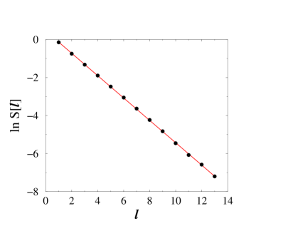
Figure 4: (Color online) Logarithmic plot of the measured degree-resolved survival probability $S[\ell]$ against degree $\ell$ for the BA network. Straight line: least-squares fit of all the data points with slope $-0.588$.

IV.3 Mass-resolved survival probability

Here, we extend our analysis to the mass-resolved survival probability of a node whose initial mass $y$ is given. Since this will only enter through the reduced mass $\alpha$, defined as the dimensionless ratio

$$\alpha=\frac{y}{\langle y\rangle},$$ (64)

we denote the mass-resolved survival probability by $S_{\alpha}$.

Along the lines of Section IV.1, we derive the following dynamical equations for the degree distribution $r_{k}(t)$ of the special node:

$$\frac{{\rm d}r_{k}(t)}{{\rm d}t} = -kr_{k}(t)$$ (65)

$$+ \lambda_{\alpha}(t)\left((k+1)r_{k+1}(t)-kr_{k}(t)\right),$$

with initial condition $r_{k}(0)=p_{k}$ (see (18)). To compute the rate $\lambda_{\alpha}(t)$ at which a random neighbor of the special node is removed, we argue as follows. This rate is a product of the probability of finding a random neighbor of degree $\ell$, given by $\widetilde{q}_{\ell}(t)=\ell q_{\ell}(t)/\langle\ell(t)\rangle$, and the rate of removal of this node. The latter is nothing but its effective degree: while the initial masses of its $\ell-1$ typical neighbors can be taken to be $\langle y\rangle$, the special node has an initial mass of $y=\alpha\langle y\rangle$, so that the effective degree of this node is $\ell-1+\alpha$. The average degree of a random neighbor of the special node at time $t$ is then clearly given by $\sum_{\ell}(\ell-1+\alpha)\widetilde{q}_{\ell}(t)$, i.e.,

$$\lambda_{\alpha}(t)=\lambda(t)-1+\alpha.$$ (66)

After some algebra, the mass-resolved survival probability reduces to:

$$S_{\alpha}=P(\zeta_{\alpha}),$$ (67)

where the mass-dependent fugacity $\zeta_{\alpha}$ is

$$\zeta_{\alpha}=1-\int_{0}^{\infty}{\rm e}^{-\alpha t-\Lambda(t)}\,{\rm d}t.$$ (68)

This formula can be recast as

$$\zeta_{\alpha}=1-\int_{\zeta}^{1}\left(1-2{\langle k\rangle}\int_{z}^{1}\frac{{\rm d}y}{P^{\prime}(y)}\right)^{(\alpha-1)/2}{\rm d}z,$$ (69)

where $\zeta$ is the fugacity given by (31). We have, consistently, $\zeta_{\alpha}=\zeta$ for $\alpha=1$.

The mass-resolved survival probability $S_{\alpha}$ is an increasing function of the reduced mass $\alpha$. We compute this explicitly for the classes of random graphs and networks considered in Section IV.1.

• ER graph. In this case, we have

  $$S_{\alpha}={\rm e}^{a(\zeta_{\alpha}-1)},$$ (70)

  with

  $$\zeta_{\alpha}=1-\frac{1}{a}\int_{0}^{a}\left(\frac{a(x+2)}{(a+2)x}\right)^{(1-\alpha)/2}\frac{{\rm d}x}{x+2}.$$ (71)

• $K$-regular graph. In this case, we have

  $$S_{\alpha}=\zeta_{\alpha}^{K},$$ (72)

  with

  $$\zeta_{\alpha}=1-\frac{1}{2}\int_{0}^{1}(2x^{2}+K(1-x^{2}))^{-(K-1)/(K-2)}x^{\alpha}{\rm d}x$$ (73)

  in the generic case ($K\geq 3$), whereas

  $$\zeta_{\alpha}=1-\int_{0}^{1}{\rm e}^{(x^{2}-1)/2}\,x^{\alpha}{\rm d}x$$ (74)

  for $K=2$.

• Geometric graph. In this case, we have

  $$S_{\alpha}=\frac{1-y}{1-y\zeta_{\alpha}},$$ (75)

  with

  $$\zeta_{\alpha}=1-\frac{1}{2}\int_{0}^{1}\left(\frac{2(1-y)}{2+(1-3x)y}\right)^{2/3}x^{(\alpha-1)/2}\,{\rm d}x.$$ (76)

• BA and GPA networks. In these cases, numerical values of $\zeta$ and of $\zeta_{\alpha}$ can be extracted from (31) and (69), using the expressions (43), (46) of the generating series $P(z)$.

The dependence of the survival probability of a node on its initial mass was computed numerically for the 1D chain, the 2D square lattice and the BA network, with an exponential mass distribution. Figure 5 shows plots of the measured values of $S_{\alpha}$ against $\alpha$. The dashed curves show the prediction (67), rescaled so as to agree with the numerics for $\alpha=1$. In the three geometries considered, the analytical prediction reproduces the overall mass dependence of $S_{\alpha}$ reasonably well. The observed dependence is slightly more pronounced than predicted on the 1D and 2D lattices, while the opposite holds for the BA network.

Figure 5: (Color online) Mass-resolved survival probability $S_{\alpha}$ against reduced mass $\alpha$. Full curves: numerical results. Corresponding dashed curves: analytical predictions. Top to bottom near $\alpha=1$: BA network, 1D chain, 2D square lattice.

Last but by no means least, there is a striking manifestation of (super-)universality in the regime of large reduced masses, when (68) simplifies to

$$\zeta_{\alpha}\approx 1-\frac{1}{\alpha}.$$ (77)

The mass-resolved survival probability then goes to unity according to the simple universal law

$$S_{\alpha}\approx 1-\frac{{\langle k\rangle}}{\alpha}.$$ (78)

This key result in the large-mass limit is one of the strongest results in this paper: all details of the structure and embeddings of networks disappear from the survival probability of a node, leaving only a simple dependence on its mass and the mean connectivity ${\langle k\rangle}$.

IV.4 Degree and mass-resolved survival probability

Finally, our analysis can be generalized to the full degree and mass-resolved survival probability $S_{\alpha}[\ell]$ of a node whose initial degree $\ell$ and reduced mass $\alpha$ are given.

The degree distribution of this special node obeys

$$\frac{{\rm d}r_{k}(t)}{{\rm d}t} = -kr_{k}(t)$$ (79)

$$+ \lambda_{\alpha}(t)\left((k+1)r_{k+1}(t)-kr_{k}(t)\right),$$

where the rate $\lambda_{\alpha}(t)$ is given by (66), and with the specific initial condition $r_{k}(0)=\delta_{k\ell}$. After some algebra along the lines of the previous sections, we find:

$$S_{\alpha}[\ell]=\zeta_{\alpha}^{\ell}.$$ (80)

This last result encompasses all the previous ones, including the expression (54) for the degree-resolved survival probability $S[\ell]$ and the expression (67) for the mass-resolved survival probability $S_{\alpha}$.

The detailed numerical evaluation of degree and mass-resolved data on networks is deferred to future work, although we expect the levels of agreement to to be similar to those obtained in Sections IV.2 and IV.3. Our point of emphasis here is the simplicity of (80), which shows that the dynamical fugacity is absolutely the right variable to highlight an intrinsic universality in this problem. In showing that the result (30) is resolvable into components of degree and mass, it also points the way towards a deeper understanding of the ‘independence’ of these parameters in the survival of a node.

Finally, and no less importantly, the result (80) again manifests (super-)universality in the regime of large reduced masses ($\alpha\gg 1$). As a consequence of (77), the degree and mass-resolved survival probability goes to unity according to the simple law

$$S_{\alpha}[\ell]\approx 1-\frac{\ell}{\alpha}.$$ (81)

The beauty of this result (as well as its analogue (78)) lies in the fact that it is exactly what one might expect intuitively; it suggests that the probability ($1-S_{\alpha}[\ell]$) that a node of mass $\alpha$ and degree $\ell$ might not survive, is directly proportional to its degree and inversely proportional to its mass. In everyday terms, the lighter the node, and the more well-connected it is, the more it is likely to disappear. The emergence of such startling, intuitive simplicity in an extremely complex system is a testament to an underlying elegance in this model.

V Discussion

The problem of finding even an approximate analytical solution to a model which contains multiple interactions is very challenging. In the context of predator-prey models, the (mean-field) Lotka-Volterra dynamical system and the full Volterra chain are among the rare examples which are integrable. Most other nonlinear dynamical models with competing interactions are not, and are quite simply intractable analytically.

The model inspired by black holes Luck and Mehta (2005), on which this paper is based, shows how competition between local and global interactions can give rise to non-trivial survivor patterns, and to the phenomenon referred to as ‘winning against the odds’. That is, a given mass can win out against more massive competitors in its immediate neighborhood provided that they in turn are ‘consumed’ by ever-more distant neighbors. When it was found numerically Thyagu and Mehta (2011); Mehta (2013); Aich and Mehta (2014) that such survivor distributions seemed to exhibit somewhat surprising features of universality, it was natural to ask the question: could one find the reasons for such behaviour, in the sense of characterizing these distributions at least approximately from an analytic point of view? An additional motivation was found in the work of the Barabási group Wang et al. (2013) on citation networks, where the authors put forward a universal scaling form for the ‘survival’ of a paper in terms of its citation history.

The black-hole model as defined in its original cosmological context Majumdar (2003); Majumdar et al. (2005) had an explicit time dependence due to the presence of a ubiquitous ‘fluid’, as well as a threshold below which even isolated particles did not survive. Neither of these attributes was necessary for the behaviour of most interest to us, namely the multiplicity of attractors (which in our case involve survivor distributions), and their non-trivial dependence on the initial mass profile, as a result of multiple interactions. One of our major achievements in this paper has been the construction of a much simpler model (without the unnecessary complications referred to above), which still retains its most interesting features from the point of view of statistical physics.

Once derived and established, this simple model was the basis of our investigations of universality in survivor distributions. The exact characterisation of attractors as a function of the initial data becoming rapidly impossible, we were led to think of approximate analytical techniques. Our choice of the inhomogeneous (or degree-based) mean-field theory was motivated by our emphasis on random graphs and networks in earlier numerical work Thyagu and Mehta (2011); Mehta (2013); Aich and Mehta (2014). This approach was embodied in an effective decimation process. Some of the analytical results so obtained were robustly universal, including the exponential fall-off (54) of the survival probability of a node with its degree, or the asymptotic behaviours (78) and (81) in the large-mass regime.

Our approach led us to introduce the associated concept of a dynamical fugacity, key to unlocking the reason behind the manifestation of universality in diverse survivor distributions. Physically, this signifies the tendency of a typical node in a network to escape annihilation, which we illustrate via a simple argument. Every time an agent encounters other, potentially predatory, agents it pays a price in terms of its survival probability: as the probability of each such encounter is independent of the others, the ‘cost’ to the total probability is multiplicative in terms of the number of predators encountered. The dynamical fugacity is then nothing but the cost function per encounter (i.e., per neighbor), so that the survival probability of the original agent depends exponentially on the number of its competitors. In a statistical sense, this depends only on the degree distribution of the chosen network, leading to the emergence of a universal survival probability for a given class of networks. The asymptotic survival probability of very heavy nodes becomes ‘super-universal’, in the sense of losing all dependence on different geometrical embeddings. Its form also has an appealing simplicity, as the complement of the ratio (degree/mass) of a given node; the heavier the node and the more isolated it is, the longer it is likely to survive.

In conclusion, we have used inhomogeneous mean-field theory to formulate and solve analytically an intractable problem with multiple interactions. While our analytical solutions are clearly not exact (due to the technical limitations of mean-field theory) they are nevertheless the only way to date of understanding the behaviour of the exact system. In particular, and importantly, our present analysis strongly reinforces the universality that has indeed been observed in earlier numerical simulations of this problem Thyagu and Mehta (2011); Mehta (2013); Aich and Mehta (2014). That such universal features emerge in a highly complex many-body problem with competing predatory interactions, is nothing short of remarkable.

Appendix A Numbers of attractors and complexity in one dimension

In this appendix we investigate the attractor statistics of the one-dimensional problem by means of the transfer-matrix formalism. We describe an attractor as a sequence of binary variables or spins:

$$\sigma_{n}=\left\{\matrix{1&\mbox{if $i$ is a survivor},\hfill\cr 0&\mbox{if $i$ is a non-survivor}.\hfill\cr}\right.$$ (82)

From a static viewpoint, attractors are defined as patterns obeying the constraints listed in Section II. They can therefore be identified with sequences which avoid the patterns 11 and 000. The last two symbols of such a sequence may therefore be 00, 01 or 10. The numbers $M_{N}^{00}$, $M_{N}^{01}$ and $M_{N}^{10}$ of attractors of length $N$ of each kind obey the recursion

$$\pmatrix{M_{N+1}^{00}\cr M_{N+1}^{01}\cr M_{N+1}^{10}}={\bf T}\pmatrix{M_{N}^{00}\cr M_{N}^{01}\cr M_{N}^{10}},$$ (83)

where the transfer matrix ${\bf T}$ reads

$${\bf T}=\pmatrix{0&0&1\cr 1&0&1\cr 0&1&0}.$$ (84)

Its characteristic polynomial is $P(x)=x^{3}-x-1$, and so the Cayley-Hamilton theorem implies the recursion

$${\bf T}^{N}={\bf T}^{N-2}+{\bf T}^{N-3}.$$ (85)

Hence all the numbers $M_{N}$ grow exponentially with $N$, in agreement with (9). The complexity reads

$$\Sigma=\ln x_{0}=0.281199,$$ (86)

with $x_{0}=1.324717$ being the largest eigenvalue of ${\bf T}$, i.e., the largest root of $P(x)$.

The total numbers of attractors $M_{N}^{({\rm c})}=M_{N}^{00}+M_{N}^{01}+M_{N}^{10}$ on chains and $M_{N}^{({\rm r})}$ on rings of $N$ nodes obey recursions derived from (85), i.e.,

$$M_{N}=M_{N-2}+M_{N-3},$$ (87)

with two different sets of initial conditions. The sequences $M_{N}^{({\rm r})}$ and $M_{N}^{({\rm c})}$ are listed in the OEIS OEIS , respectively as entries A001608 and A000931, together with many combinatorial interpretations and references. The first few terms are listed in Table 2.

$N$	$\ 1\$	$\ 2\$	$\ 3\$	$\ 4\$	$\ 5\$	$\ 6\$	$\ 7\$	$\ 8\$	$\ 9\$	$\ 10\$	$\ 11\$	$\ 12\$
$M_{N}^{({\rm r})}$	0	2	3	2	5	5	7	10	12	17	22	29
$M_{N}^{({\rm c})}$	1	2	2	3	4	5	7	9	12	16	21	28

Table 2: Numbers of attractors $M_{N}^{({\rm r})}$ on rings and $M_{N}^{({\rm c})}$ on chains of $N$ nodes, for $N$ up to 12.

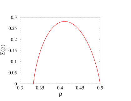
Figure 6: (Color online) Density-dependent static complexity $\Sigma(\rho)$ against survivor density $\rho$ in the allowed range ($1/3\leq\rho\leq 1/2$).

The transfer-matrix approach can be generalized in order to determine the density-dependent static complexity $\Sigma(\rho)$, characterizing the exponential growth of the number of attractors with a fixed density $\rho$ of survivors. Introducing a static fugacity $z$ conjugate to the number of survivors, the transfer matrix becomes

$${\bf T}(z)=\pmatrix{0&0&1\cr z&0&z\cr 0&1&0},$$ (88)

whose characteristic polynomial is $P(z,x)=x^{3}-zx-z$. The reader is referred to de Smedt et al. (2002); Godrèche and Luck (2005) for details. We obtain after some algebra

$$\Sigma(\rho)=-(1-2\rho)\ln\frac{1-2\rho}{\rho}-(3\rho-1)\ln\frac{3\rho-1}{\rho}.$$ (89)

Figure 6 shows a plot of this quantity against survivor density in the allowed range ($1/3\leq\rho\leq 1/2$). The expression (89) reaches a maximum equal to $\Sigma$ (see (86)) when $\rho$ equals the mean static density of survivors:

$$\rho_{0}=\frac{x_{0}+1}{2x_{0}+3}=0.411495.$$ (90)

References

- Murray (1989) J. D. Murray, Mathematical Biology (Springer, Berlin, 1989).
- Berryman (1992) A. A. Berryman, Ecology 73, 1530 (1992).
- Szabó and Fáth (2007) G. Szabó and G. Fáth, Phys. Rep. 446, 97 (2007).
- Majumdar (2003) A. S. Majumdar, Phys. Rev. Lett. 90, 031303 (2003).
- Majumdar et al. (2005) A. S. Majumdar, A. Mehta, and J. M. Luck, Phys. Lett. B 607, 219 (2005).
- Luck and Mehta (2005) J. M. Luck and A. Mehta, Eur. Phys. J. B 44, 79 (2005).
- Thyagu and Mehta (2011) N. N. Thyagu and A. Mehta, Physica A 390, 1458 (2011).
- Aich and Mehta (2014) S. Aich and A. Mehta, Eur. Phys. J. Special Topics 223, 2745 (2014).
- Mehta (2013) A. Mehta, in Econophysics of Systemic Risk and Network Dynamics, edited by F. Abergel, B. K. Chakrabarti, A. Chakraborti, and A. Ghosh (Springer, Milan, 2013), New Economic Windows, pp. 141–156.
- Mehta et al. (2005) A. Mehta, A. S. Majumdar, and J. M. Luck, in Econophysics of Wealth Distributions, edited by A. Chatterjee, B. K. Chakrabarti, and S. Yarlagadda (Springer, Milan, 2005), pp. 199–204.
- Jenks (1969) R. D. Jenks, J. Diff. Equations 5, 497 (1969).
- Li (2003) J. B. Li, Int. J. Bif. Chaos 13, 47 (2003).
- Thouless et al. (1977) D. J. Thouless, P. W. Anderson, and R. G. Palmer, Phil. Mag. 35, 593 (1977).
- Kirkpatrick and Sherrington (1978) S. Kirkpatrick and D. Sherrington, Phys. Rev. B 17, 4384 (1978).
- Stillinger and Weber (1982) F. H. Stillinger and T. A. Weber, Phys. Rev. A 25, 978 (1982).
- Kirkpatrick and Wolynes (1987) T. R. Kirkpatrick and P. G. Wolynes, Phys. Rev. A 35, 3072 (1987).
- Franz and Virasoro (2000) S. Franz and M. A. Virasoro, J. Phys. A 33, 891 (2000).
- Edwards (1994) S. F. Edwards, in Granular Matter: An Interdisciplinary Approach, edited by A. Mehta (Springer, New York, 1994).
- Dean and Lefèvre (2001) D. S. Dean and A. Lefèvre, Phys. Rev. Lett. 86, 5639 (2001).
- Berg and Mehta (2001) J. Berg and A. Mehta, Europhys. Lett. 56, 784 (2001).
- Prados and Brey (2001) A. Prados and J. J. Brey, Phys. Rev. E 66, 041308 (2001).
- de Smedt et al. (2002) G. de Smedt, C. Godrèche, and J. M. Luck, Eur. Phys. J. B 27, 363 (2002).
- Godrèche and Luck (2005) C. Godrèche and J. M. Luck, J. Phys. Cond. Matter 17, S2573 (2005).
- Mikhailov et al. (1987) A. V. Mikhailov, A. B. Shabat, and R. I. Yamilov, Russian Math. Surveys 42, 1 (1987).
- Yamilov (2006) R. Yamilov, J. Phys. A 39, R541 (2006).
- Evans (1993) J. W. Evans, Rev. Mod. Phys. 65, 1281 (1993).
- Pastor-Satorras and Vespignani (2001) R. Pastor-Satorras and A. Vespignani, Phys. Rev. Lett. 86, 3200 (2001).
- Barrat et al. (2008) A. Barrat, M. Barthélemy, and A. Vespignani, Dynamical Processes on Complex Networks (Cambridge University Press, Cambridge, 2008).
- Pastor-Satorras et al. (2015) R. Pastor-Satorras, C. Castellano, P. van Mieghem, and A. Vespignani, Rev. Mod. Phys. 87, 925 (2015).
- Feller (1966) W. Feller, An Introduction to Probability Theory and its Applications (Wiley, New York, 1966).
- Erdös and Rényi (1959) P. Erdös and A. Rényi, Publ. Mathematicae 6, 290 (1959).
- Erdös and Rényi (1960) P. Erdös and A. Rényi, Publ. Math. Inst. Hungar. Acad. Sci. 5, 17 (1960).
- Barabási and Albert (1999) A. L. Barabási and R. Albert, Science 286, 509 (1999).
- Barabási et al. (1999) A. L. Barabási, R. Albert, and H. Jeong, Physica A 272, 173 (1999).
- Dorogovtsev et al. (2000) S. N. Dorogovtsev, J. Mendes, and A. Samukhin, Phys. Rev. Lett. 85, 4633 (2000).
- Krapivsky et al. (2000) P. L. Krapivsky, S. Redner, and F. Leyvraz, Phys. Rev. Lett. 85, 4629 (2000).
- Godrèche et al. (2009) C. Godrèche, H. Grandclaude, and J. M. Luck, J. Stat. Phys. 137, 1117 (2009).
- Krapivsky and Redner (2001) P. L. Krapivsky and S. Redner, Phys. Rev. E 63, 066123 (2001).
- Krapivsky and Redner (2002) P. L. Krapivsky and S. Redner, J. Phys. A 35, 9517 (2002).
- Wang et al. (2013) D. Wang, C. Song, and A. L. Barabási, Science 342, 127 (2013).
- (41) OEIS, The On-Line Encyclopedia of Integer Sequences, URL http://oeis.org.