A novel computation of the thermodynamics of the SU($3$) Yang-Mills theory

Abstract:

We present an accurate computation of the Equation of State of the SU(3) Yang-Mills theory using shifted boundary conditions in the temporal direction. In this framework, the entropy density $s$ can be obtained in a simple way from the expectation value of the space-time components $T_{0k}$ of the energy-momentum tensor. At each given value of the temperature, $s$ is measured in an independent way at several values of the lattice spacing. The extrapolation to the continuum limit shows small discretization effects with respect to the statistical errors of approximatively 0.5$\%$.

1 Introduction

The pressure, $p$, the energy density, $e$, and the entropy density $s$, are main features of Quantum Chromo Dynamics (QCD) at finite temperature $T$. The Equation of State describes the temperature dependence of the above quantities, and it is of crucial relevance in many areas. It is an important input in the analysis of data collected at the heavy-ion colliders, in the study of nuclear matter, and in astrophysics and cosmology when strongly interacting matter is under extreme conditions. Many collaborations have put a lot of effort in calculating the thermodynamics features of QCD by numerical simulations on the lattice, both in the pure gauge sector and with dynamical fermions. These studies are challenging from the numerical viewpoint: $p$, $e$, and $s$ are related to the free energy density which suffers from an ultraviolet additive power-divergent renormalization, and cannot be directly measured in a Monte Carlo simulation.

In Ref. [1] a first accurate investigation of the Equation of State of the SU($3$) Yang-Mills theory was accomplished by numerical simulations on the lattice. This approach has turned out to be very successful; however it has the drawback that a subtraction at $T=0$, or at some other temperature [2], has to be performed. Interestingly, there are also other equations that relate the pressure, the energy density and the entropy density to the expectation values of the matrix elements of the energy-momentum tensor $T_{\mu\nu}$  [3]. A practical use of those equations in Monte Carlo simulations on the lattice, however, requires the computation of the renormalization constants of the bare lattice tensor [4, 5, 6].

The energy-momentum tensor contains the currents associated to Poincaré symmetry and scale transformations. As a consequence, when the regularization of a quantum theory preserves space-time symmetries – like, for instance, dimensional regularization – $T_{\mu\nu}$ does not renormalize. The lattice regularization explicitly breaks the Poincaré invariance, which is recovered only in the continuum limit. Thus, the bare energy-momentum tensor needs to be properly renormalized to guarantee that the associated charges generate translations and rotations in the continuum limit [4]. For the Yang-Mills theory, scale invariance is also broken by the regularization; however, that symmetry is anomalous and it is not restored in the continuum limit, generating a dynamical mass-gap.

The proper approach to define non-perturbatively the renormalized energy-momentum tensor on the lattice is to impose the validity of some Ward Identities at fixed lattice spacing up to terms that vanish in the continuum limit [4]. Based on that framework, the renormalization constants of $T_{\mu\nu}$ have been computed in perturbation theory at 1 loop [7]. Although one can in principle construct a lattice definition of the energy-momentum tensor, the non-perturbative calculation of the renormalization factors can be not straightforward if one has to consider correlation functions that are difficult to measure by numerical simulations.

A few years ago, a thermal quantum field theory has been formulated in a moving reference frame using the path-integral language [8, 5, 6]. This setup can be implemented by considering a spatial shift ${\bm{\xi}}$ when closing the boundary conditions along the temporal direction. The shift ${\bm{\xi}}$ corresponds to the Wick rotation of the speed of the moving frame. Interestingly, in this new framework, one can write down new Ward Identities involving the energy-momentum tensor, that allow to compute in a simple way the non-perturbative renormalization factors of the energy-momentum tensor on the lattice [6, 9]. Furthermore, since the shift breaks explicitly the parity symmetry, there are new equations relating the thermodynamic quantities and the expectation values of off-diagonal matrix element of $T_{\mu\nu}$. Numerical simulations with shifted boundary conditions have already provided new successful, simple methods to study the thermodynamics of the Yang-Mills theory [10].

This report is organized as follows. In section 2, the main equations with shifted boundary conditions are summarized both in the continuum and on the lattice. The next section presents the results of the non-perturbative calculation of the renormalization factors of the energy-momentum tensor and, in section 4, the renormalized energy-momentum tensor is used to compute the Equation of State of the SU($3$) Yang-Mills theory. Conclusions and outlook follow.

2 Ward Identities with shifted boundary conditions

We consider the thermal SU($3$) Yang-Mills theory in the Euclidean space in the path-integral formulation with shifted boundary conditions [6]

$$A_{\mu}(L_{0},\bm{x})=A_{\mu}(0,\bm{x}-L_{0}\bm{\xi})\;,$$ (1)

where $L_{0}$ is the system size along the compact direction and $\bm{\xi}\in\mathbb{R}^{3}$ is the shift. When $\bm{\xi}\neq 0$, the parity symmetry is broken, and there are new interesting Ward Identities involving the energy-momentum tensor $T_{\mu\nu}$ [8, 5, 6] ($x_{0}\neq 0$)

$$L_{0}\langle\;T_{0k}\rangle_{\bm{\xi}}=\frac{1}{V}\frac{\partial}{\partial\xi_{k}}\ln Z(L_{0},\bm{\xi})\;,\qquad L_{0}\langle\;{\overline{T}}_{0k}(x_{0})\,O(0)\rangle_{\bm{\xi},\,c}=\frac{\partial}{\partial\xi_{k}}\langle O\rangle_{\bm{\xi}}\;.$$ (2)

The functional $Z(L_{0},\bm{\xi})$ is the partition function with shifted boundary conditions, and $O$ is a generic gauge invariant operator. The subscript $c$ indicates a connected correlation function, $\langle\cdot\rangle_{{\bm{\xi}}}$ stands for the expectation value with shifted boundary conditions, and ${\overline{T}}_{\mu\nu}=\int d^{3}x\,T_{\mu\nu}(x)$. The field $T_{\mu\nu}$ can be defined by

$$T_{\mu\nu}(x)=\frac{1}{g_{0}^{2}}\left[F_{\mu\rho}^{a}(x)F_{\nu\rho}^{a}(x)-\frac{1}{4}\delta_{\mu\nu}F_{\rho\sigma}^{a}(x)F_{\rho\sigma}^{a}(x)\right]\;,$$ (3)

where $g_{0}$ is the bare coupling constant. The field strength is given in terms of the gauge field $A_{\mu}(x)$ by $F_{\mu\nu}(x)=\partial_{\mu}A_{\nu}(x)-\partial_{\nu}A_{\mu}(x)-i[A_{\mu}(x),A_{\nu}(x)]$. Other useful equations are the following [6, 9]

$$\langle T_{0k}\rangle_{\bm{\xi}}=\frac{\xi_{k}}{1-\xi_{k}^{2}}\left\{\langle T_{00}\rangle_{\bm{\xi}}-\langle T_{kk}\rangle_{\bm{\xi}}\,\right\}\;,\qquad\frac{\partial}{\partial\xi_{k}}\langle T_{\mu\mu}\rangle_{\bm{\xi}}=\frac{1}{(1+\xi^{2})^{2}}\frac{\partial}{\partial\xi_{k}}\left[\frac{(1+\xi^{2})^{3}}{\xi_{k}}\langle T_{0k}\rangle_{\bm{\xi}}\right]\;.$$ (4)

It is important to note that the above equations involve the expectation value of the off-diagonal matrix element $\langle T_{0k}\rangle$, which may be non vanishing due to the breaking of parity symmetry.

When we consider the lattice regularization, the 10-dimensional symmetric $SO(4)$ representation of the energy-momentum tensor splits into the sum of the sextet, the triplet, and the singlet irreducible representations of the hyper-cubic group. The field $T_{\mu\nu}$ can then be expressed as a combination of the following three operators

$$T^{[1]}_{\mu\nu}=(1-\delta_{\mu\nu})\frac{1}{g_{0}^{2}}F^{a}_{\mu\alpha}F^{a}_{\nu\alpha}\;,\;\;T^{[2]}_{\mu\nu}=\delta_{\mu\nu}\,\frac{1}{4g_{0}^{2}}\,F^{a}_{\alpha\beta}F^{a}_{\alpha\beta}\;,\;\;T^{[3]}_{\mu\nu}=\delta_{\mu\nu}\frac{1}{g_{0}^{2}}\Big{\{}F^{a}_{\mu\alpha}F^{a}_{\mu\alpha}-\frac{1}{4}F^{a}_{\alpha\beta}F^{a}_{\alpha\beta}\Big{\}}\;,$$ (5)

and of the identity. Since translation and rotation symmetries are broken by the lattice, the sextet $T^{[1]}_{\mu\nu}$ and the triplet $T^{[3]}_{\mu\nu}$ operators pick up a multiplicative renormalization factor only, while the singlet $T^{[2]}_{\mu\nu}$ mixes also with the identity. The renormalized energy-momentum tensor can finally be written as $T^{\rm R}_{\mu\nu}=Z_{{}_{T}}\Big{\{}T^{[1]}_{\mu\nu}+z_{{}_{T}}T^{[3]}_{\mu\nu}+z_{{}_{S}}\big{[}T^{[2]}_{\mu\nu}-\langle T^{[2]}_{\mu\nu}\rangle_{0}\big{]}\Big{\}}$ .

Because of the finite renormalization factors, we can write the lattice version of the first equation of (2) as follows

$$Z_{{}_{T}}(g_{0}^{2})=-\frac{\Delta f}{\Delta\xi_{k}}\,\frac{1}{\langle T^{[1]}_{0k}\rangle_{\bm{\xi}}}\;,\qquad\mbox{with}\quad\frac{\Delta f}{\Delta\xi_{k}}=\frac{1}{2aV}\ln\Big{[}\frac{Z(L_{0},{\bm{\xi}}-a\hat{k}/L_{0})}{Z(L_{0},{\bm{\xi}}+a\hat{k}/L_{0})}\Big{]}.$$ (6)

The two equations in (4) become

$$z_{{}_{T}}(g_{0}^{2})=\frac{1-\xi_{k}^{2}}{\xi_{k}}\frac{\langle T^{[1]}_{0k}\rangle_{\bm{\xi}}}{\langle T^{[3]}_{00}\rangle_{\bm{\xi}}-\langle T^{[3]}_{kk}\rangle_{\bm{\xi}}}\;,$$ (7)

$$z_{{}_{S}}=\frac{1}{(1+\xi^{2})^{2}}\frac{\left[\frac{(1+\xi^{{}^{\prime}2})^{3}}{\xi^{\prime}_{k}}\langle T^{[1]}_{0k}\rangle_{\bm{\xi}^{\prime}}\right]_{\bm{\xi}^{\prime}=\bm{\xi}+a\hat{k}/L_{0}}-\left[\frac{(1+\xi^{{}^{\prime}2})^{3}}{\xi^{\prime}_{k}}\langle T^{[1]}_{0k}\rangle_{\bm{\xi}^{\prime}}\right]_{\bm{\xi}^{\prime}=\bm{\xi}-a\hat{k}/L_{0}}}{\langle T^{[2]}_{\mu\mu}\rangle_{\bm{\xi}+a\hat{k}/L_{0}}-\langle T^{[2]}_{\mu\mu}\rangle_{\bm{\xi}-a\hat{k}/L_{0}}}\;.$$ (8)

Note that the equations (6)–(8) allow for a fully non-perturbative definition of $T_{\mu\nu}$. They also suggest simple procedures to perform the numerical calculations of $Z_{{}_{T}}$, $z_{{}_{T}}$ and $z_{{}_{S}}$ since only the expectation values of local fields need to be measured.

3 The non-perturbative renormalization factors

In this section we present the results of Monte Carlo simulations to calculate $Z_{{}_{T}}(g_{0}^{2})$ and $z_{{}_{T}}(g_{0}^{2})$ in the range $g_{0}^{2}\in(0,1)$ [9]; work is in progress for the computation of $z_{{}_{S}}(g_{0}^{2})$. We define the SU($3$) Yang–Mills theory on a space-time lattice of volume $L_{0}\times L^{3}$ and lattice spacing $a$. We impose periodic boundary conditions in the spatial directions and shifted boundary conditions in the compact one: $U_{\mu}(L_{0},\bm{x})=U_{\mu}(0,\bm{x}-L_{0}\bm{\xi})$, where $U_{\mu}(x_{0},\bm{x})$ are the link variables. We consider the standard Wilson action $S[U]=-1/g_{0}^{2}\,\sum_{x,\mu\nu}{\rm Re}\mbox{Tr}[U_{\mu\nu}(x)]$, where the plaquette is given by $U_{\mu\nu}(x)=U_{\mu}(x)\,U_{\nu}(x+a\hat{\mu})\,U^{\dagger}_{\mu}(x+a\hat{\nu})\,U^{\dagger}_{\nu}(x)$. The gluon field strength tensor is defined as [4]

$$F^{a}_{\mu\nu}(x)=-\frac{i}{4a^{2}}\mbox{Tr}\Big{\{}\Big{[}Q_{\mu\nu}(x)-Q_{\nu\mu}(x)\Big{]}T^{a}\Big{\}}\;,$$ (9)

where $Q_{\mu\nu}(x)=U_{\mu\nu}(x)+U_{\nu-\mu}(x)+U_{-\mu-\nu}(x)+U_{-\nu\mu}(x)$, and the minus sign stands for the negative orientation. The renormalization constants $Z_{{}_{T}}$, $z_{{}_{T}}$ and $z_{{}_{S}}$ are finite, and depend on $g^{2}_{0}$ only up to discretization effects. Considering the above definition of the field strength tensor on the lattice, at 1 loop in perturbation theory their expressions are [4, 7]

$$Z_{{}_{T}}(g_{0}^{2})=1+0.27076\;g_{0}^{2}\;,\quad z_{{}_{T}}(g_{0}^{2})=1-0.03008\;g_{0}^{2}\;,\quad z_{{}_{S}}(g_{0}^{2})=\frac{b_{0}}{2}g_{0}^{2}\;.$$ (10)

3.1 Computation of $Z_{{}_{T}}$

The direct determination of $\Delta f/\Delta\xi_{k}$ in Eq. (6) is a numerically challenging problem since it requires the computation of the ratio of two partition functions with a poor overlap of the relevant phase space [11, 12, 8].

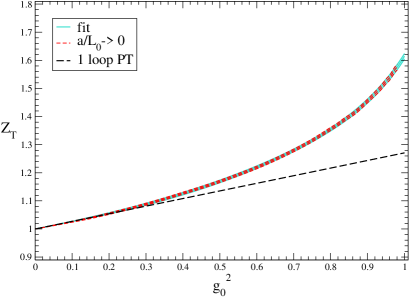
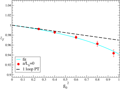
Figure 1: The renormalization factor $Z_{{}_{T}}(g_{0}^{2})$ (left panel) and $z_{{}_{T}}(g_{0}^{2})$ (right panel) as a function of the bare coupling $g_{0}^{2}$. The dashed lines represent the 1-loop perturbative results, while the solid ones are interpolating fits of the numerical data.

Moreover, the calculation becomes quickly demanding for large lattices because the numerical cost increases quadratically with the spatial volume. Since $\Delta f/\Delta\xi_{k}$ is a smooth function of $g_{0}^{2}$ at fixed values of $L_{0}/a$ and $L/a$ in the range of chosen values, its derivative with respect to $g_{0}^{2}$ can be written as

$$\frac{d}{dg_{0}^{2}}\frac{\Delta f}{\Delta\xi_{k}}=\frac{1}{2aL^{3}g_{0}^{2}}\,\Big{\{}\langle S\rangle_{{\bm{\xi}}-a/L_{0}\hat{k}}-\langle S\rangle_{{\bm{\xi}}+a/L_{0}\hat{k}}\Big{\}}\;.$$ (11)

The difference in the r.h.s. has been computed for ${\bm{\xi}}=(1,0,0)$ and $L/a=48$ at $L_{0}/a=3,4$ and $5$ for many values of $g_{0}^{2}$. At each value of $L_{0}/a$ the points are interpolated with a cubic spline, and the resulting curve is integrated over $g_{0}^{2}$. The free-case value is computed analytically and is added to the integral. Then $\langle T^{[1]}_{0k}\rangle_{\bm{\xi}}$ has also been computed at many values of $g_{0}^{2}$ and the results have been interpolated with cubic splines. The final result for $Z_{{}_{T}}$ is shown in the left panel of Fig. 1 together with the 1-loop perturbative result, and an interpolating fit gives

$$Z_{{}_{T}}(g_{0}^{2})=\frac{1-0.4457\,g_{0}^{2}}{1-0.7165\,g_{0}^{2}}-0.2543\,g_{0}^{4}+0.4357\,g_{0}^{6}-0.5221\,g_{0}^{8}\;.$$ (12)

3.2 Determination of $z_{{}_{T}}$

The renormalization constant $z_{{}_{T}}$ is calculated by imposing the tree-level improved version of Eq. (7) given by $\{z_{{}_{T}}(g_{0}^{2})-\mbox{ free case}\}$ , with $\frac{L\,\xi_{k}}{L_{0}(1+\xi_{k}^{2})}=q\in\mathbb{Z}$. The expectation values of $\langle T^{[1]}_{0k}\rangle_{\bm{\xi}}$ and of the difference $\langle T^{[3]}_{00}\rangle_{\bm{\xi}}-\langle T^{[3]}_{kk}\rangle_{\bm{\xi}}$ are measured straightforwardly in the same simulation.

We chose ${\bm{\xi}}=(1/2,0,0)$ and $q=8$ so that the ratio of the spatial linear size over the temporal one is fixed to be $L/L_{0}=20$. We simulated 5 values of $g_{0}^{2}$ in the range $0\leq g_{0}^{2}\leq 1$ with temporal length $L_{0}/a=4,6,8$ and $12$. After performing a combined extrapolation to $a/L_{0}=0$, the final results are shown in the right panel of Fig. 1. The dashed line is the 1-loop perturbative result, and the solid one is an interpolating fit which gives

$$z_{{}_{T}}(g_{0}^{2})=\frac{1-0.5090\,g_{0}^{2}}{1-0.4789\,g_{0}^{2}}\;.$$ (13)

4 The Equation of State

In this section we use the non-perturbative calculation of the renormalization factors of the energy-momentum tensor to obtain the Equation of State from Monte Carlo simulations. With shifted boundary conditions, the entropy density $s$ can be written as [6]

$$\frac{s}{T^{3}}=-\frac{L_{0}^{4}(1+{\bf\xi}^{2})^{3}}{\xi_{k}}\langle T_{0k}\rangle_{\xi}Z_{T},$$ (14)

where $T=1/L_{0}\sqrt{1+{\bf\xi}^{2}}$ is the temperature. In Ref. [10] the temperature dependence of $s/T^{3}$ has been measured using the step-scaling function: in that approach one can avoid computing $Z_{T}$ at all temperature values , but only fixed constant steps in $T$ can be done. However, once the renormalization factor $Z_{T}$ is known, the Eq. (14) allows to measure $s/T^{3}$ directly at any temperature.

We have performed numerical simulations at 21 different temperatures in the range between $T_{c}$ and 7.5 $T_{c}$, where $T_{c}$ is the critical temperature of the theory. For each temperature we extrapolate $s/T^{3}$ to the continuum limit by considering $L_{0}/a=5,6,7,8$ and, sometimes, also $L_{0}/a=3,4$ and 10. The extrapolation is performed independently for every temperature, and we barely see discretization effects within the numerical accuracy (see left plot of Fig. 2). The spatial volume has been chosen to be $L/a=128$ for $L_{0}/a=3,4,5,6$ and $L/a=256$ for $L_{0}/a=7,8,10$. Except for one point with shift $\bm{\xi}=(1,1,1)$, we have always considered $\bm{\xi}=(1,0,0)$. The scale is set using the Sommer scale [13, 14], $r_{0}$, for $T<1.9\;T_{c}$ and $L_{max}$ for higher temperatures [15].

In Fig. 2 we compare our preliminary data with the results available in the literature. In the region $1$-$2.5~{}T_{c}$ our data are compatible with those in Ref. [1] that have significantly larger errors, while we find a statistically significant discrepancy with the more precise ones in Ref. [2]. At larger temperatures, up to $T\simeq 7\;T_{c}$, our results agree with those presented in Ref. [2]. Work is in progress to clarify the above mentioned discrepancy, and to reach temperatures of about $250~{}T_{c}$.

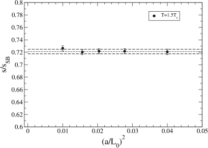
Figure 2: Left: continuum limit extrapolation for $s/T^{3}$ computed as in Eq. (14) at $T=1.5T_{c}$. Right: the temperature dependence of the dimensionless ratio $s/T^{3}$ in the continuum limit; the results obtained using Eq. (14) are compared with data available in the literature.

5 Conclusions and outlook

We have presented preliminary results of a new computation of the Equation of State of the SU($3$) Yang-Mills theory. The computational strategy uses shifted boundary conditions in the compact direction, and it can be applied in a straightforward way to a generic SU($N$) Yang-Mills theory as well as to theories with dynamical fermions. The approach relies on the non-perturbative calculation of the renormalization factors of the energy-momentum tensor. The framework of shifted boundary conditions turns out to be very effective and simple to investigate the Yang-Mills theory at finite temperature. Work is in progress to include also dynamical fermions.

References

- [1] G. Boyd, J. Engels, F. Karsch, E. Laermann, C. Legeland, M. Lutgemeier and B. Petersson, Nucl. Phys. B 469, 419 (1996).
- [2] S. Borsanyi, G. Endrodi, Z. Fodor, S. D. Katz and K. K. Szabo, JHEP 1207, 056 (2012).
- [3] L. Landau and E. Lifshitz, Course of Theoretical Physics VI: Fluid Mechanics, Butterworth-Heinemann (1987).
- [4] S. Caracciolo, G. Curci, P. Menotti and A. Pelissetto, Annals Phys. 197, 119 (1990).
- [5] L. Giusti and H. B. Meyer, JHEP 1111, 087 (2011).
- [6] L. Giusti and H. B. Meyer, JHEP 1301, 140 (2013).
- [7] S. Caracciolo, P. Menotti and A. Pelissetto, Nucl. Phys. B 375, 195 (1992).
- [8] L. Giusti and H. B. Meyer, Phys. Rev. Lett. 106, 131601 (2011).
- [9] L. Giusti and M. Pepe, Phys. Rev. D 91, 114504 (2015).
- [10] L. Giusti and M. Pepe, Phys. Rev. Lett. 113, 031601 (2014).
- [11] P. de Forcrand, M. D’Elia and M. Pepe, Phys. Rev. Lett. 86, 1438 (2001).
- [12] M. Della Morte and L. Giusti, Comput. Phys. Commun. 180, 813 (2009).
- [13] R. Sommer, Nucl. Phys. B 411, 839 (1994) [hep-lat/9310022].
- [14] S. Necco and R. Sommer, Nucl. Phys. B 622, 328 (2002) [hep-lat/0108008].
- [15] S. Capitani et al. [ALPHA Collaboration], Nucl. Phys. B 544, 669 (1999) [hep-lat/9810063].