Velocity Statistics of the Nagel-Schreckenberg Model

Abstract

The statistics of velocities in the cellular automaton model of Nagel and Schreckenberg for traffic Nagel and Schreckenberg (1992) are studied. From numerical simulations, we obtain the probability distribution function (PDF) for vehicle velocities and the velocity-velocity (vv) correlation function. We identify the probability to find a standing vehicle as a potential order parameter that signals nicely the transition between free congested flow for sufficiently large number of velocity states. Our results for the vv correlation function resemble features of a second order phase transition. We develop a $3$-body approximation that allows us to relate the PDFs for velocities and headways. Using this relation, an approximation to the velocity PDF is obtained from the headway PDF observed in simulations. We find a remarkable agreement between this approximation and the velocity PDF obtained from simulations.

I Introduction

Traffic flow theory is the backbone for understanding and improving the mobility of people and goods in our road network. The classical tool to characterizing mobility (in either field tests or from simulations) is by plotting flow vs. density in form of the so-called fundamental diagram (Fig.1) for both individual road segments and road networks Schadschneider et al. ; to separate free flow patterns below a critical density from congested flow patterns above. While empirical approaches, based on equilibrium concepts, link vehicle speed to density, eventually enriched by information related to human behavior Chowdhury et al. (2000), the fundamental structure of the transition from free to congested flow remains a topical issue, which may ultimately reconcile the considerable scatter in field experiments with traffic flow theory and simulation. This provides ample motivation for us to study velocity distribution functions of a specific class of traffic models, cellular automata models (CA), that are known to exhibit two different phases (free and congested flow) and a transition between them Gerwinski and Krug (1999). Specifically, we herein investigate the velocity distribution functions for a simple version of these models, namely the Nagel-Schreckenberg (NaSch) model for one lane traffic Nagel and Schreckenberg (1992). The model is based on the discretization of the road into cells of the size of a single vehicle, and the whole system is described as the ensemble $(v_{1},...,v_{N},d_{1},...,d_{N})$ of velocities $v_{j}$ and headways $d_{j}$ (number of empty cells in front of a vehicle) of $N$ vehicles Nagel and Schreckenberg (1992); Schreckenberg et al. (1995). The time evolution of the vehicles’ positions $x_{j}$ and velocities $v_{j}$ follows four distinct update rules:

1. Acceleration: $v_{j}=\min(v_{j}+1,v_{max})$

2. Deceleration: $v_{j}=\min(d_{j},v_{j})$

3. Random deceleration: $v_{j}=\max(v_{j}-1,0)$ with a probability $p$

4. Movement: $x_{j}\rightarrow x_{j}+v_{j}$

Herein, the velocity $v_{max}$, a model parameter, corresponds to the maximum velocity that a vehicle can reach when there are no slower vehicles ahead. The stochastic parameter $p$ represents the probability that a vehicle randomly slows down, and aims at capturing the lack of perfection in human behavior. In practice, the parameters $v_{max}$ and $p$ are kept constant, while the total density of vehicles $\rho$ is varied, which is the number of vehicles divided by the number of cells. For convenience, the physical dimensions of headway and vehicle position are expressed in unit of cells, and the velocity in unit of cells per iteration time step; thus omitting the time dimension so that velocities and distances have formally the same dimension.

The NaSch model has been studied through mean-field (MF) theories for which velocity distribution functions were computed Schreckenberg et al. (1995). Since MF theories fail to give simple and accurate results for values of $v_{max}>2$, our study of the probability distribution function (PDF) for velocities of the NaSch model is based on both numerical simulations and exact results for a simplified 3-body approximation. To obtain the PDF, we analyze in detail the $v_{max}+1$ different accessible single vehicle velocity states between $0$ and $v_{max}$. We choose a value of $v_{max}=10$ which ensures obtaining a sufficiently large number of states; and which is of the order of magnitude of typical highway speeds. The stochastic parameter is chosen to be $p=0.5$ and remains constant throughout the study. In order to avoid finite size effects we run simulations with periodic boundary conditions over $2\times 10^{4}$ cells for $10^{6}$ iteration time steps to reduce the influence of transient behavior. To probe the effect of different initial conditions we initialized the system in three distinct ways:

• Megajam: block of $N$ standing vehicles Gerwinski and Krug (1999)

• Equally spaced, standing vehicles Barlovic et al. (1998)

• Equally spaced vehicles moving with $v_{max}$

Our results turned out to be independent of these initial conditions, unless mentioned explicitly later in the text.

As already noted, the NaSch model exhibits two different phases (free and congested flow) and a transition between them with a yet to be defined order parameter Schadschneider et al. . Specifically, in the deterministic case ($p=0$), a sharp phase transition occurs at a critical density $\rho_{c}=1/(v_{max}+1)$ that coincides with the density of maximum flow $j=\rho\langle v\rangle$, where $\langle v\rangle$ is the mean velocity of all vehicles, averaged over time. It has been a subject of intense debate in recent literature if the NaSch model exhibits a similar sharp transition in the presence of randomness ($p>0$). In Section II we shed new light on this still open key question by analyzing the statistics of velocities. We identify an approximate “order parameter”, and study the “transition” by looking at the velocity-velocity correlation function. In Section III we show that the PDF for velocities and headways cannot be obtained straightforwardly from the parameters of the model since there are no separate PDFs in the free and jammed flow. Based on this insight thus gained, we develop, in Section IV, an exact solution for a 3-body approximation. This approximation is employed in Section V to provide estimates for the velocity PDF from the knowledge of the PDF for headways. The paper concludes with a summary and discussion of our findings.

II Potential “order parameter” and velocity correlations

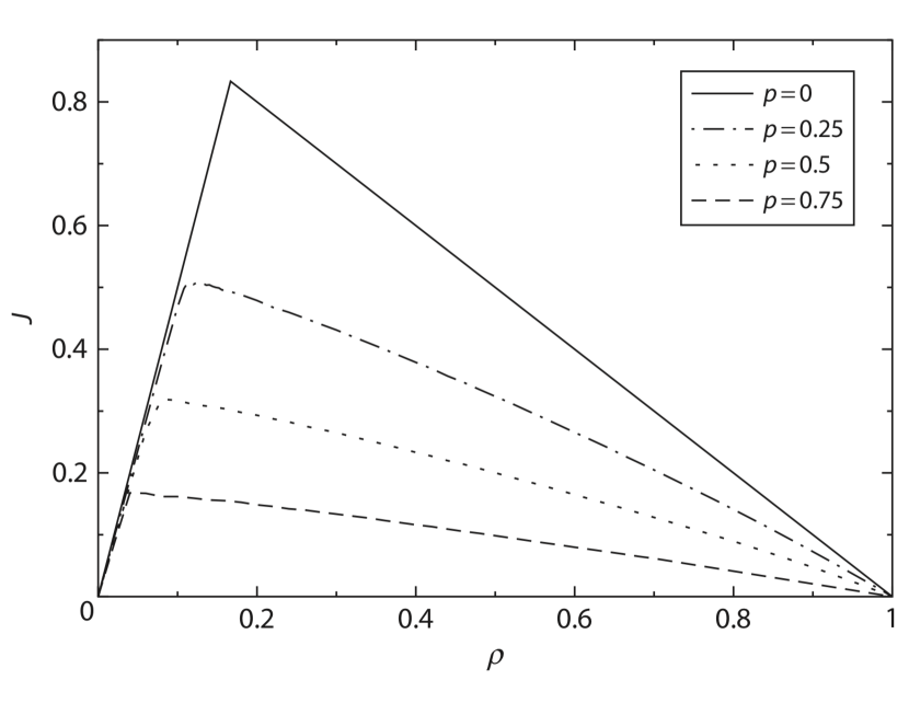
Figure 1: Numerically obtained fundamental diagrams of the NaSch model with $v_{max}=5$ for different values of the stochastic parameter $p$. (flow $j$ in arbitrary units.) Taken from Ref. Schadschneider et al. .

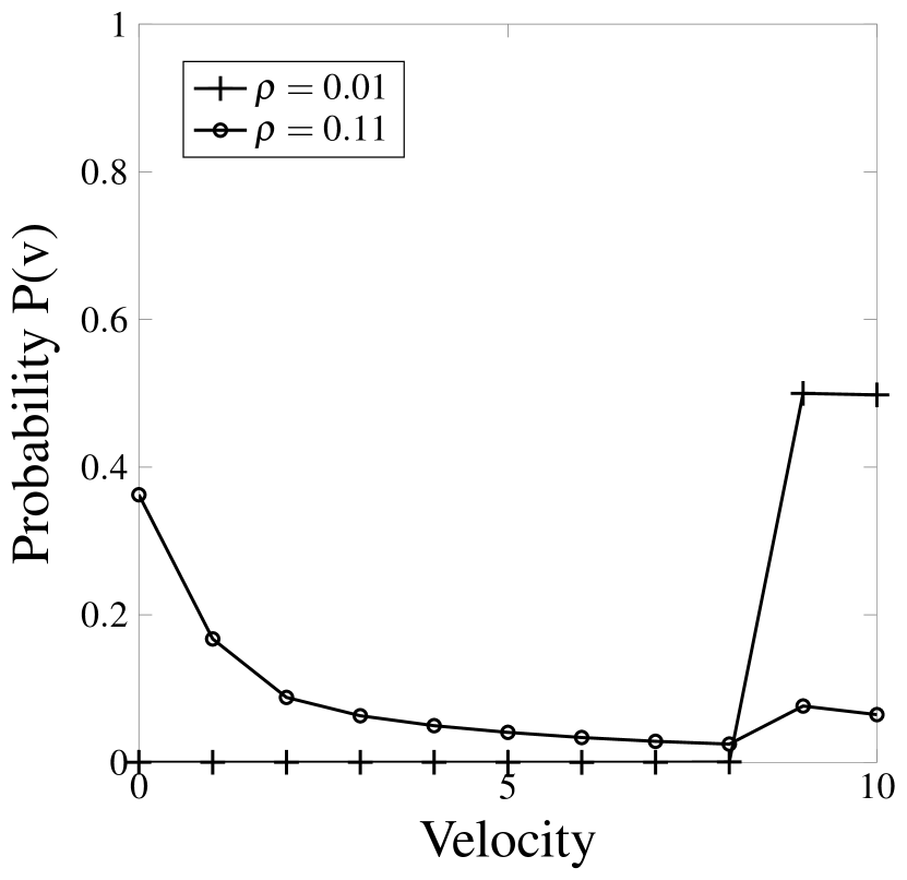
Figure 2: Velocity PDFs in both the free and congested flow phase. The PDF for freely flowing vehicles is non-zero only for $v_{max}$ with value $1-p$ and $v_{max}-1$ with value $p$. In the congested regime the probability to find a standing vehicle is finite, signaling the presence of traffic jams.

The NaSch model with randomness exhibits some kind of transition when going from low to high densities. Below the transition, there exists a free flow regime in which the interactions between vehicles are negligible and the flow $j$ increases linearly with density. Above the transition, one encounters a congested regime in which the flow $j$ decreases with increasing density. The flow-density relation, usually referred to as fundamental diagram, hence clearly shows a transition. Examples for the NaSch model for $v_{max}=5$ and different values of the stochastic parameter $p$ are shown in Fig. 1. One might expect the existence of a genuine phase transition but it is not straightforward to define a corresponding order parameter because it is not obvious what symmetry is broken at the transition. To address this point, we inspect the PDF for velocities, $P(v)$. Averaging over all simulation time steps, we find two very distinct distributions in the two phases (Fig. 2). In the free flow phase, the vehicles do not interact and every vehicle can travel either at velocity $v_{max}$ or $v_{max}-1$ with some negligible interactions. This solution is exactly known from the update rules, from taking the limit $d_{j}>v_{max}$. In the congested phase the probability to find a standing vehicle is strictly non-zero, $P(v=0)>0$, and the probability to have a vehicle at velocity $v_{max}$ or $v_{max}-1$ decays with increasing density. The numerical result for $P(v=0)$ as a function of density is shown in Fig. 3 for the initial condition (I2). The curve shows a clear drop to zero at a density $\rho_{c}\approx 0.036$. This suggest that $P(v=0)$ could be an order parameter for a putative phase transition between free and congested flow. However, it has been argued in Ref. Gerwinski and Krug (1999) that for small densities $\rho\to 0$ one has the scaling $P(v=0)\sim\rho^{v_{max}-1}$ showing that $P(v=0)$ is non-zero at any density, and hence cannot serve as an order parameter in general. This can be reconciled with our observation for $v_{max}=10$ by studying the behavior of $P(v=0)$ for smaller $v_{max}$ which is shown in the insets of Fig. 3. While for $v_{max}=2$ there is indeed a continuos variation of $P(v=0)$ with a change of curvature close to the critical density (density of maximum flow) found in Ref. Gerwinski and Krug (1999), already for $v_{max}=5$ there is a rather steep drop in $P(v=0)$ very close to the critical density of Ref. Gerwinski and Krug (1999), see also Fig. 1 for $p=0.5$. Our observations suggest that $P(v=0)$ can be considered as an approximate or effective “order parameter” that describes the transition rather well for sufficiently large $v_{max}$. We argue that in a continuum version of the NaSch model with an infinite number $v_{max}\to\infty$ of discrete velocity states, $P(v=0)$ becomes a genuine order parameter. This order parameter is different from previously adopted choices such as the number of vehicles in the high local density phases Lübeck et al. (1998), the density of nearest-neighbor pairs at rest Chowdhury et al. (2000), or the deviation of the mean velocity from the velocity of free-moving vehicles Gerwinski and Krug (1999). The data for $P(v=0)$ are the only ones in our numerical study that slightly depend on the initial conditions, presumably due to the vicinity to the critical density. However, the results for $v_{max}=10$ always show a discontinuity around $\rho_{c}$. The behavior could be an artefact of finite simulation time, but this problem seems unavoidable because of the divergence of the time needed to reach a steady state close to $\rho_{c}$ Gerwinski and Krug (1999).

To gain a better understanding of the system’s behavior at the transition, we study the velocity-velocity correlation function

$$G_{v}(r)=\frac{1}{NT}\sum\limits_{t=1}^{T}\sum\limits_{j=1}^{N}v_{j}(t)v_{j+r}(t)-\langle v\rangle^{2}$$ (1)

where $T$ is the simulation time, whereas $\langle v\rangle$ denotes the average, over time and vehicles, of the individual vehicle velocities $v_{j}(t)$ at time step $t$:

$$\langle v\rangle=\frac{1}{NT}\sum\limits_{j=1}^{N}\sum\limits_{t=1}^{T}v_{j}(t)\,,$$ (2)

We observe, in Fig. 4, three distinct behaviors of the velocity-velocity correlation function: (1) Well below the critical density, at $\rho=0.01$, we find no correlation in the velocity of successive vehicles [Fig. 4(a)]. This is consistent with a free flow in which all vehicles behave independently from each another. (2) Well above the critical point, at $\rho=0.21$, [Fig. 4(c)], we observe an exponential decay with a correlation number of $r_{c}\approx 4$ successive vehicles [Fig. 4(d)] which is characteristic of short-range correlations. (3) Just above the critical density, at $\rho=0.05$, we find a nearly linear decay of the correlation function, suggesting a diverging correlation number $r_{c}$ [Fig. 4(b)]. This divergence of the correlation number close to the critical density mimics a second-order phase transition.

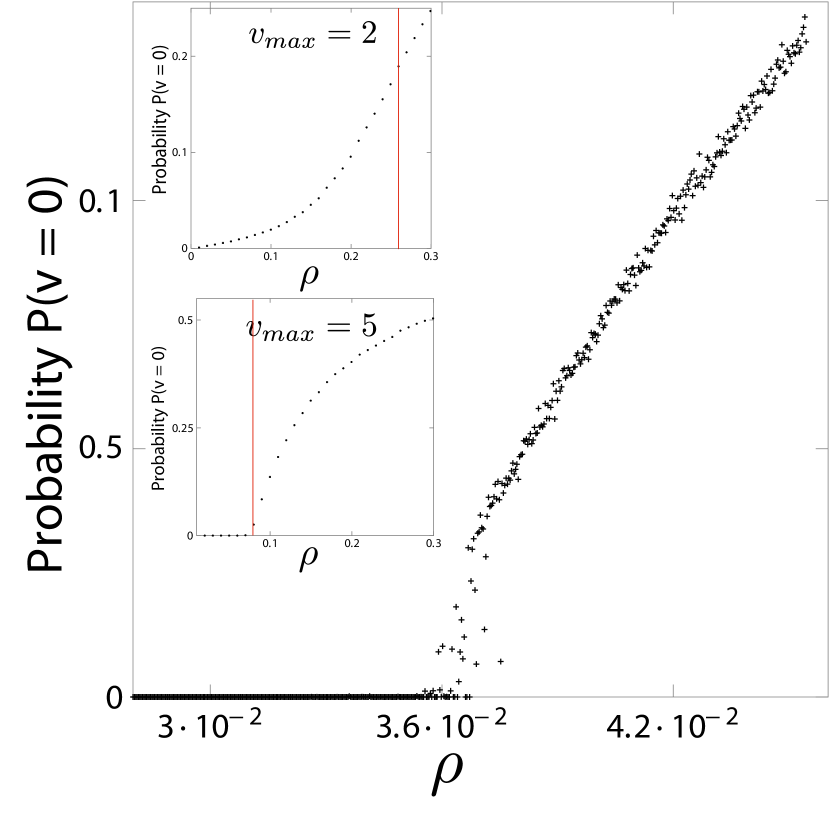
Figure 3: Probability to find a standing vehicle, $P(v=0)$ as function of the average density, for a system initialized with equally spaced, standing vehicles, and $v_{max}=10$. The critical density is close to $\rho_{c}=0.036$. Insets: $P(v=0)$ for two smaller $v_{max}$ with the critical densities obtained numerically in Ref. Gerwinski and Krug (1999) marked by vertical lines.

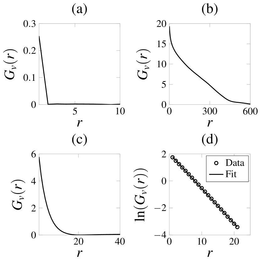
Figure 4: Velocity-velocity correlation function [see Eq. (1)] as a function of the vehicle number $r$ in the free flow regime (a), just above the critical density $\rho_{c}$ (b), and well above the critical density (c). Shown in (d) is also a logarithmic plot of the velocity-velocity correlation function well above the critical density fitted with a line corresponding to a correlation number $r_{c}\approx 4$.

III PDF of velocities

The PDF of the velocities, as shown in Fig. 2, might suggest that the PDFs for velocities and headways could be computed as the sum of a PDF for the jammed phase ($P_{J}$ and $Q_{J}$, respectively) and a PDF for free flow phase ($P_{F}$ and $Q_{F}$, respectively), weighted by the proportion of the number of vehicles in each phase. This scheme has been proposed in Ref. Krauss et al. (1996). When $\omega$ is the fraction of vehicles in the free flow phase, this superposition assumption yields the following PDF for velocities:

$$P(v)=\omega P_{F}(v)+(1-\omega)P_{J}(v)\,.$$ (3)

This form is convenient if one wants to predict velocity or headway PDFs from a given density. To check the validity of this hypothesis, we computed numerically the headway and velocity PDFs at different densities in two regimes: below the critical density $\rho_{c}$ representative of the free flow state; and well above the critical density $\rho_{c}$ where no vehicles are in the free flow state. The resulting PDFs in the free flow phase are shown in Fig. 5. According to Eq. (3) the distributions should be independent of density. While this seems to be true for the velocity PDF, for the distribution of headways this is clearly not the case. This observation shows that the superposition model expressed by (3) is but an oversimplification of the true behavior of the model. It suggests that the internal structure of the traffic state quite certainly plays a role in the shape of the headway and velocity PDFs. One therefore needs a new method to predict velocity and headway distributions for the NaSch model.

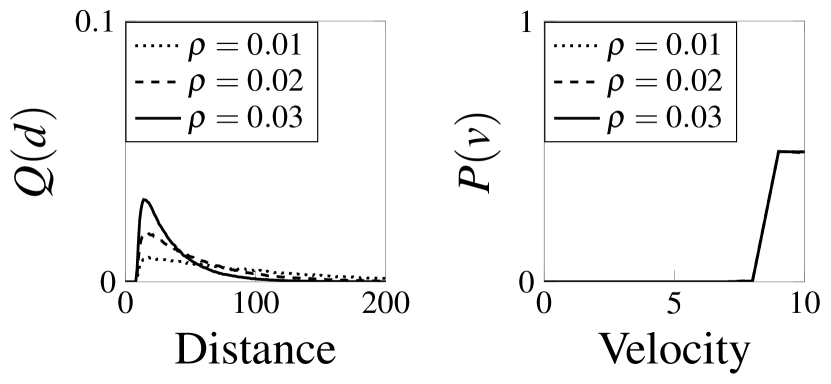
Figure 5: Velocity and headway PDFs for three different densities in the free flow phase. The velocity distributions $P(v)$ are independent of these densities but the headway distributions $Q(d)$ show a strong dependence on density.

IV A $3$-body approximation: Exact solution

We approach this problem analytically, by considering a $3$-body approximation for the NaSch model for which an exact analytical solution is derived. To this end, consider a standing vehicle which we number as $j=0$. Assume that this vehicle represents the tail of a jam and that it remains stopped. At a distance $d_{0}$ behind this vehicle we place a second vehicle, $j=1$, and a third one, $j=2$ in the cell immediately behind vehicle $j=1$, both initially standing. This is the initial configuration. Then compute at every iteration step the joint PDF $P(d_{1},v_{1},d_{2},v_{2},t|d_{0})$ which is the probability to find at time $t$ vehicle $j=1$ at a distance $d_{1}$ from vehicle $j=0$ at velocity $v_{1}$, and to find vehicle $j=2$ at a distance $d_{2}$ from vehicle $j=1$ and velocity $v_{2}$. This joint PDF $P$ is calculated iteratively from the initial conditions

$$P(d_{1},v_{1},d_{2},v_{2},t|d_{0})=\delta_{d_{1},d_{0}}\delta_{v_{1},0}\delta_{d_{2},0}\delta_{v_{2},0}$$ (4)

with $\delta_{a,b}$ the Kronecker delta. The time evolution of this PDF is determined by iteration rules that depend on different regimes of distances between the three vehicles. In the simplest case of sufficiently large distances, with the definition $P_{a,b}=P(d_{1}+a,a,d_{2}-a+b,b,t-1|d_{0})$, the iteration rule can be written as

$$P(d_{1},v_{1},d_{2},v_{2},t|d_{0}) =ppP_{v_{1},v_{2}}+pqP_{v_{1},v_{2}-1}$$ (5)

$$+qpP_{v_{1}-1,v_{2}}+qqP_{v_{1}-1,v_{2}-1}$$

with $q=1-p$. The precise form of the other iteration rules (5) slightly differ in the conditions on $d_{1}$, $v_{1}$, $d_{2}$ and $v_{2}$; and we refer for details to Appendix A. From this joint distribution, the PDF of a given variable is obtained by summing over all other variables. For instance, the velocity PDF $p_{1}(v_{1},t|d_{0})$ of vehicle $j=1$ at time $t$ reads as:

$$p_{1}(v_{1},t|d_{0})=\sum\limits_{d_{1}=0}^{d_{0}}\sum\limits_{d_{2}=0}^{d_{0}}\sum\limits_{v_{2}=0}^{v_{max}}P(d_{1},v_{1},d_{2},v_{2},t|d_{0})\,.$$ (6)

The time evolution of this PDF for $d_{0}=500$ is plotted in Fig. 6 for all $v_{max}+1$ velocity states. From the probabilities for the different velocities $v_{1}$, we recognize three distinct phases; namely acceleration, free flow, and deceleration.

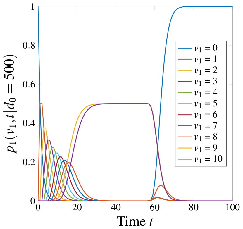
Figure 6: Time evolution of the PDF $p_{1}(v_{1},t|d_{0})$ of vehicle $1$ for all possible velocities and for an initial spacing $d_{0}=500$. We notice three distinct regimes in the time evolution of the probability to find vehicle $1$ at velocity $v_{1}$. First the vehicle accelerates, corresponding to a decrease of the probability that it stands. Next, the occurence of finite probabilities for intermediate velocities, signalling a transition to free flow with equally likely velocities $v_{max}-1$ and $v_{max}$. Eventually, deceleration when vehicle $1$ approaches the tail of the jam, corresponding to probability $1$ to find the vehicle standing.

V Application: relating headway and velocity distributions

In the previous section we developed an exact solution for PDFs within a $3$-body approximation. We now investigate how this result can be used to link headway and velocity PDFs in the congested state. For this purpose, we base the reasoning on our observation that in a congested state the probability to find a standing vehicle is non-vanishing, see Section II. Therefore, if one takes a snapshot of a congested state at a given time, one observes standing vehicles with moving vehicles in between them. We start by focusing on these standing vehicles and the ones directly ahead of them, and hence on the constrained headway PDF of any stopped vehicle $Q_{n}(d_{i}|v_{i}=0)$, and the constrained velocity PDF of any vehicle which is followed by a stopped vehicle $P_{n}(v_{j}|v_{j+1}=0)$. While these two distributions can be obtained from our numerical simulation results with the NaSch model, we herein aim at obtaining an approximation $P_{m}(v_{1}|v_{2}=0)$ for this constrained velocity PDF within the $3$-body approximation. We thus relate $P_{m}(v_{1}|v_{2}=0)$ to the numerically obtained headway PDF $Q_{n}(d_{i}|v_{i}=0)$. By comparing the approximate to the numerically obtained velocity PDF, we can probe the accuracy of the $3$-body approximation. In order to relate the numerically computed headway distribution $Q_{n}(d_{i}|v_{i}=0)$ to the $3$-body approximation, we assume that a congested state can be described as a succession of $3$-body blocks with a PDF $Q_{0}(d_{0})$ for the initial spacing $d_{0}$. We define the summed probabilities

$$\begin{split}D_{m}(d_{2},d_{0})&=\sum\limits_{t=0}^{T}\sum\limits_{d_{1}=0}^{d_{0}}\sum\limits_{v_{1}=0}^{v_{max}}P(d_{1},v_{1},d_{2},0,t|d_{0})\\ V_{m}(v_{1},d_{0})&=\sum\limits_{t=0}^{T}\sum\limits_{d_{1}=0}^{d_{0}}\sum\limits_{d_{2}=0}^{d_{0}}P(d_{1},v_{1},d_{2},0,t|d_{0})\end{split}$$ (7)

which can be viewed as matrices with row index $d_{2}$ (or $v_{1}$) and column index $d_{0}$. This allows us to express the headway distribution $Q_{m}(d_{2}|v_{2}=0)$ of vehicle $2$ when it remains standing as

$$Q_{m}(d_{2}|v_{2}=0)=D_{m}.Q_{0}=Q_{n}(d_{i}|v_{i}=0)$$ (8)

Similarly, we can easily obtain the velocity PDF of vehicles followed by a standing vehicle as

$$P_{m}(v_{1}|v_{2}=0)=V_{m}.Q_{0}=V_{m}.(D_{m})^{-1}.Q_{n}(d_{i}|v_{i}=0)$$ (9)

Note that the matrix $D_{m}$ is invertible because it is triangular with non-vanishing diagonal elements. A comparison of the constrained velocity PDF obtained respectively from simulations, $P_{n}(v_{j}|v_{j+1}=0)$, and analytically with the $3$-body approximation, $P_{m}(v_{1}|v_{2}=0)$, is plotted in Fig. 7 for a density of $\rho=0.21$, and shows a fairly good agreement achieved without any adjustable fitting parameters. Worthnoty in this plot is the significant difference between the constrained and the unconstrained velocity PDFs, $P_{n}(v_{j}|v_{j+1}=0)$ and $P_{n}(v)$, which underlines the limitations of mean-field theories. Note also, that in order to keep the total iteration time $T$ small enough, we use the velocity and headway distributions for moving vehicles only, i.e., excluding zero velocity and headway.

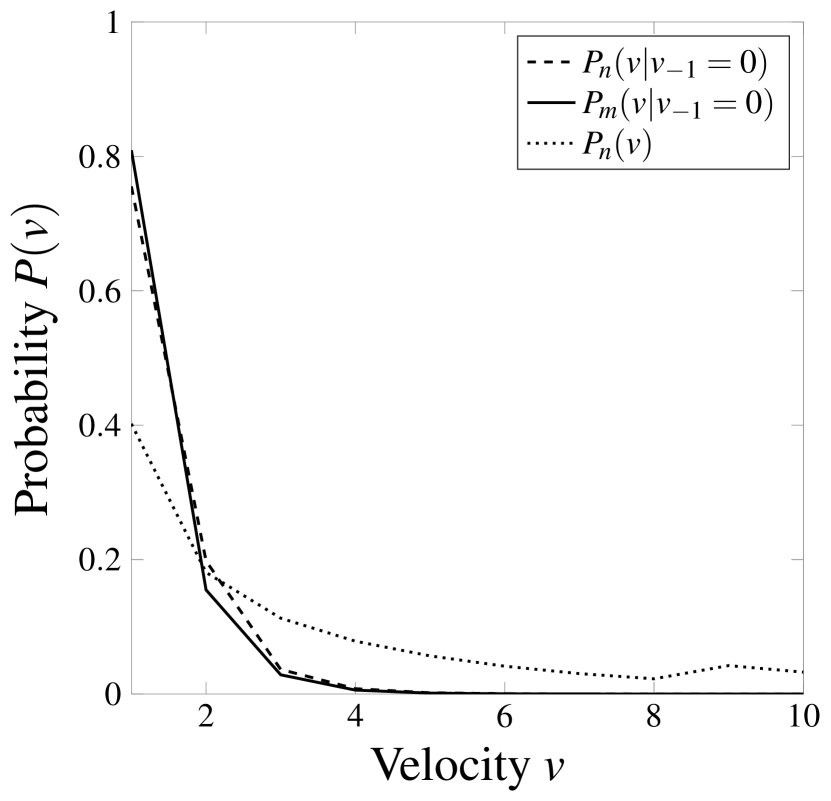
Figure 7: Velocity PDFs $P_{n}$ obtained numerically in the constrained and unconstrained case, and the velocity PDF $P_{m}$ obtained from the headway distribution and the three-body approximation in the constrained case. The density is fixed at $\rho=0.21$.

Next, we investigate how to relate the unconstrained velocity and headway PDFs that we obtained numerically, by using the three-body approximation. To do so, one has to estimate the global headway PDF from the headway distributions of the two vehicles $j=1,\,2$ of the $3$-body blocks. First, we define the headway PDFs as the matrices

$$\begin{split}\hat{D}_{m,1}(d,d_{0})&=\sum\limits_{t,v_{1},d_{2},v_{2}}P(d,v_{1},d_{2},v_{2},t|d_{0})\\ \hat{D}_{m,2}(d,d_{0})&=\sum\limits_{t,d_{1},v_{1},v_{2}}P(d_{1},v_{1},d,v_{2},t|d_{0})\,.\end{split}$$ (10)

Next, we introduce a parameter $\alpha$ to approximate the global headway distribution as a superposition of the ones for the two vehicles,

$$\hat{D}_{m}=(1-\alpha)\hat{D}_{m,1}+\alpha\hat{D}_{m,2}\,.$$ (11)

Finally, we define the velocity PDFs

$$\begin{split}\hat{V}_{m,1}=(v,d_{0})&=\sum\limits_{t,d_{1},d_{2},v_{2}}P(d_{1},v,d_{2},v_{2},t|d_{0})\\ \hat{V}_{m,2}=(v,d_{0})&=\sum\limits_{t,d_{1},d_{2},v_{1}}P(d_{1},v_{1},d_{2},v,t|d_{0})\,.\end{split}$$ (12)

Since we have $\hat{V}_{m,1}\approx\hat{V}_{m,2}$, we will simply set $\hat{V}_{m}=\hat{V}_{m,1}$. We note that this approximation is justified since the velocity of vehicle $j=2$ is essentially the same as the one of vehicle $j=1$, but shifted in time. This does not hold for the headway distributions since the initial spacing between vehicles $j=1$ and $j=0$ is significantly different from the one between vehicles $j=2$ and $j=1$. Now we can use Eqs. (8), (9) with $D_{m}$ replaced by $\hat{D}_{m}$ and $V_{m}$ replaced by $\hat{V}_{m}$ to obtain an approximation for the unconstrained velocity PDF $P(v)$ from the simulation result for the headway PDF $Q_{n}(d|v=0)$. This approximation is now compared to the velocity PDF obtained from the simulations where $\alpha$ is used as a fitting parameter. The results are shown in Fig. 8 for the choices $\alpha=0$, $\alpha=0.5$ and $\alpha=0.95$ for a fixed density $\rho=0.21$. One observes a remarkable agreement between the PDFs obtained respectively from our numerical simulations and the $3$-body approximation applied to the simulation result for the headway distribution when the fitting parameter is $\alpha=0.95$. The physical meaning of the fitting parameter, however, is not immediately obvious. A possible interpretation is the following. The basic assumption for the approximation presented here is that a congested state can be considered at any time step as a distribution of standing vehicles with moving vehicles in between them. In our $3$-body approximation there is always a pair of moving vehicles ($j=1,\,2$) that approaches the tail of a jammed region (vehicle $j=0$). Hence, one can view $\alpha$ as the relative importance of the distribution of the distance between the two vehicles of a pair, and $1-\alpha$ as the relative importance of the distribution of the distance between a moving pair and the tail of the jam ahead. Our comparison in Fig. 8 then suggests that the velocity PDF in a jammed state is much more sensitive to the constrained distribution of the distances between two moving vehicles approaching a standing vehicle than the distribution of actual distances of the pair to the standing vehicle. This in turn suggests that the velocity PDF in a congested state is mostly determined by the dynamics within regions of still moving vehicles and not the interaction of these regions with jammed regions.

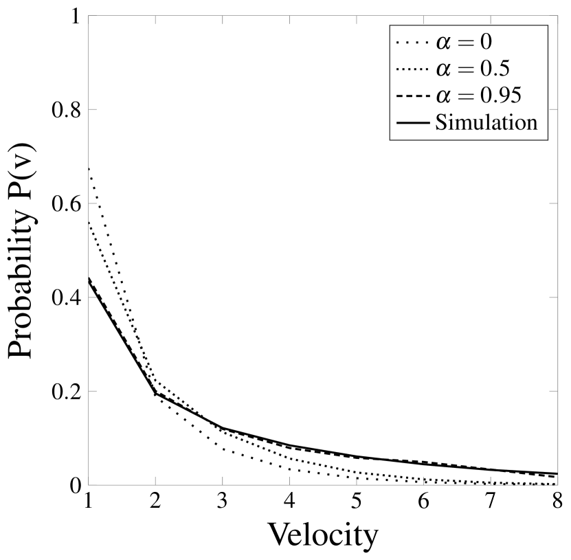
Figure 8: Approximate results for the velocity PDF for different values of the fitting parameter $\alpha$ (dashed and dotted lines), and the velocity PDF obtained from simulations for a density $\rho=0.21$.

VI Conclusion

In this paper we analyzed the statistics of velocities in the NaSch model. We studied the characteristics of the two phases and the phase transition in between them. We find that in the free flow phase the interactions between vehicles are negligible and that the velocity PDF assumes a simple form. The congested phase is characterized by a non-zero probability to find a standing vehicle. We suggest to use this probability as an approximate “order parameter” that might become a genuine order parameter in a continuum version of the model where $v_{max}\to\infty$ velocity states exist. The nature of the phase transition could not be fully determined. There seems to be a discontinuity at a critical density but this could be an artefact of a too short simulation time. The velocity-velocity correlation function shows three different regimes: Free flow with no correlation in velocity, a critical regime with diverging correlation number and highly congested flow with a short correlation number. This scenario resembles a second order phase transition.

Our simulations show that all PDFs are highly dependent on the density, whether in free flow or in the completely congested regime, with the exception of a simple PDF for the velocities in the low-density free flow. We presented an analytical solution for a three-body approximation, that allowed us to analytically link the headway and velocity distribution functions. We first focused on a constrained case with stopped vehicles, and then studied the unconstrained case. This approximation describes nicely the constrained case. By introducing a fitting parameter in the constrained case, we could also reach a remarkable agreement between simulation results and our approximation. An attempt to interpret the physical meaning of the fitting parameter has been made. The method presented in this paper to link headway and velocity PDFs could prove useful to link other quantities of interest and to learn more about the local dynamics in the jammed phase.

In addition to offering a new perspective on traffic models, the present study of velocity statistics might help identifying the nature of a potential phase transition in the stochastic NaSch model. Moreover, in more applied terms, the knowledge of velocity distributions enables one to compute expected excess fuel consumption related to road properties as the ones studied in Refs. Louhghalam et al. (2013, 2014, 2015) as a function of traffic conditions, which is the topic of a forthcoming paper. This relation opens new perspectives, alongside with the recent boom of data collections Fazeen et al. (2012), which enables one to revisit traffic models and adapt them to meet the requirements of other research areas like, e.g., carbon management.

Appendix A Details of the $3$-body approximation

In order to obtain the complete iteration rules of the $3$-body interaction approximation we introduce the notion of limiting speed $\hat{v}_{j}=\min(d_{j},v_{max})$, which is the speed that the vehicle $j$ cannot exceed at any given time. For each vehicle we have to distinguish three cases:

• $v_{j}<\hat{v}_{j}-1$

• $v_{j}=\hat{v}_{j}-1$

• $v_{j}=\hat{v}_{j}$

with the assumption that $d_{j}>1$, the case $d_{j}=0$ being trivial. The indices $1$ and $2$ being interchangeable, we denote six different cases:

1. $v_{1}<\hat{v}_{1}-1$ and $v_{2}<\hat{v}_{2}-1$

2. $v_{1}=\hat{v}_{1}-1$ and $v_{2}<\hat{v}_{2}-1$

3. $v_{1}=\hat{v}_{1}$ and $v_{2}<\hat{v}_{2}-1$

4. $v_{1}=\hat{v}_{1}-1$ and $v_{2}=\hat{v}_{2}-1$

5. $v_{1}=\hat{v}_{1}$ and $v_{2}=\hat{v}_{2}-1$

6. $v_{1}=\hat{v}_{1}$ and $v_{2}=\hat{v}_{2}$

Finally we introduce the scalar variables:

$$r_{j}=\left\{\begin{array}[]{ll}p\mbox{ if }v_{j}<\hat{v}_{j}&\\ q\mbox{ if }v_{j}=\hat{v}_{j}&\end{array}\right.\,;\,s_{j}=\left\{\begin{array}[]{ll}q\mbox{ if }v_{j}>0&\\ 0\mbox{ if }v_{j}=0&\end{array}\right.$$ (13)

With that in hand we write the iteration rule for all the cases. Case (1) is the most simple and given in Eq. (5). Cases (2) and (3) can be grouped together and follow the iteration rule:

$$P=r_{1}\sum\limits_{w_{1}=v_{1}}^{v_{max}}\left(r_{2}P_{w_{1},v_{2}}+s_{2}P_{w_{1},v_{2}-1}\right)$$

$$\quad+s_{1}r_{2}P_{v_{1}-1,v_{2}}+s_{1}s_{2}P_{v_{1}-1,v_{2}-1}$$ (14)

with $P=P(d_{1},v_{1},d_{2},v_{2},t|d_{0})$. As for cases (4), (5) and (6), they also can be grouped in the same iteration rule, in the form:

$$P=r_{1}\sum\limits_{w_{1}=v_{1}}^{v_{max}}\left(r_{2}\sum\limits_{w_{2}=v_{2}}^{v_{max}}P_{w_{1},w_{2}}+s_{2}P_{w_{1},v_{2}-1}\right)$$

$$\quad+s_{1}r_{2}\sum\limits_{w_{2}=v_{2}}^{v_{max}}P_{v_{1}-1,w_{2}}+s_{1}s_{2}P_{v_{1}-1,v_{2}-1}$$ (15)

Implementing these iteration rules numerically is tedious but not technically difficult, and enables one to retrieve the results described in Section (IV).

Bibliography

- Nagel and Schreckenberg (1992) K. Nagel and M. Schreckenberg, Journal de physique I 2, 2221 (1992).
- (2) A. Schadschneider, D. Chowdhury, and K. Nishinari, Stochastic transport in complex systems: from molecules to vehicles (Elsevier).
- Chowdhury et al. (2000) D. Chowdhury, L. Santen, and A. Schadschneider, Physics Reports 329, 199 (2000).
- Gerwinski and Krug (1999) M. Gerwinski and J. Krug, Physical Review E 60, 188 (1999).
- Schreckenberg et al. (1995) M. Schreckenberg, A. Schadschneider, K. Nagel, and N. Ito, Physical Review E 51, 2939 (1995).
- Barlovic et al. (1998) R. Barlovic, L. Santen, A. Schadschneider, and M. Schreckenberg, The European Physical Journal B-Condensed Matter and Complex Systems 5, 793 (1998).
- Lübeck et al. (1998) S. Lübeck, M. Schreckenberg, and K. Usadel, Physical Review E 57, 1171 (1998).
- Krauss et al. (1996) S. Krauss, P. Wagner, and C. Gawron, Physical Review E 54, 3707 (1996).
- Louhghalam et al. (2013) A. Louhghalam, M. Akbarian, and F.-J. Ulm, Journal of Engineering Mechanics 140 (2013).
- Louhghalam et al. (2014) A. Louhghalam, M. Akbarian, and F.-J. Ulm, Transportation Research Record: Journal of the Transportation Research Board 2457, 95 (2014).
- Louhghalam et al. (2015) A. Louhghalam, M. Akbarian, and F.-J. Ulm, in Transportation Research Board 94th Annual Meeting (2015).
- Fazeen et al. (2012) M. Fazeen, B. Gozick, R. Dantu, M. Bhukhiya, and M. C. González, Intelligent Transportation Systems, IEEE Transactions on 13, 1462 (2012).