Combined first-principles and model Hamiltonian study
of the perovskite series $R$MnO₃ ($R$ = La, Pr, Nd, Sm, Eu and Gd)

Abstract

We merge advanced ab initio schemes (standard density functional theory, hybrid functionals and the GW approximation) with model Hamiltonian approaches (tight-binding and Heisenberg Hamiltonian) to study the evolution of the electronic, magnetic and dielectric properties of the manganite family $R$MnO₃ ($R$ = La, Pr, Nd, Sm, Eu and Gd). The link between first principles and tight-binding is established by downfolding the physically relevant subset of $3d$ bands with $e_{g}$ character by means of maximally localized Wannier functions (MLWFs) using the VASP2WANNIER90 interface. The MLWFs are then used to construct a general tight-binding Hamiltonian written as a sum of the kinetic term, the Hund’s rule coupling, the JT coupling, and the electron-electron interaction. The dispersion of the TB $e_{g}$ bands at all levels are found to match closely the MLWFs. We provide a complete set of TB parameters which can serve as guidance for the interpretation of future studies based on many-body Hamiltonian approaches. In particular, we find that the Hund’s rule coupling strength, the Jahn-Teller coupling strength, and the Hubbard interaction parameter $U$ remain nearly constant for all the members of the $R$MnO₃ series, whereas the nearest neighbor hopping amplitudes show a monotonic attenuation as expected from the trend of the tolerance factor. Magnetic exchange interactions, computed by mapping a large set of hybrid functional total energies onto an Heisenberg Hamiltonian, clarify the origin of the A-type magnetic ordering observed in the early rare-earth manganite series as arising from a net negative out-of-plane interaction energy. The obtained exchange parameters are used to estimate the Néel temperature by means of Monte Carlo simulations. The resulting data capture well the monotonic decrease of the ordering temperature down the series from $R$ = La to Gd, in agreement with experiments. This trend correlates well with the modulation of structural properties, in particular with the progressive reduction of the Mn-O-Mn bond angle which is associated with the quenching of the volume and the decrease of the tolerance factor due to the shrinkage of the ionic radii of $R$ going from La to Gd.

I Introduction

Perovskite transition metal oxides (TMOs), which fall under the category of strongly correlated systems, exhibit a wide array of complex orbitally and spin ordered states, arising from the interplay of the structural, electronic and magnetic degrees of freedom. In particular, rare earth manganites with the general formula $R_{1-x}A_{x}$MnO₃, where $R$ is a trivalent rare earth cation and $A$ is a divalent alkaline earth cation, exhibit stunning characteristics such as the colossal magnetoresistance (CMR) effect von Helmolt et al. (1993); Salamon and Jaime (2001); Khomskii and Sawatzky (1997); Kusters et al. (1989); Jin et al. (1994), observed in compounds like Pr_1-xCa_xMnO₃, Pr_1-xBa_xMnO₃, Nd_0.5Sr_0.5MnO₃ and in the well-known hole-doped LaMnO₃ Tokura et al. (1994); Zener (1951). Another interesting property, tuned by the Mn³⁺ magnetic structure variation in $R$MnO₃ Kimura et al. (2003), is the emergence of magneto-electric/multiferroic properties for the smaller rare earth cations ($R=$ Gd, Tb, Dy) Goto et al. (2004); Kimura et al. (2005). Despite the large number of studies on CMR and parent CMR compounds, experimental Sánchez et al. (2003); Ferreira et al. (2009); Chatterji et al. (2009); Muñoz et al. (2000); Kamegashira and Miyazaki (1983); Dabrowski et al. (2005); Laverdière et al. (2006); Iliev et al. (2006); Lee et al. (2009); Iyama et al. (2012) and theoretical studies Yamauchi et al. (2008); Kim and Min (2009); Moskvin et al. (2010); Dong et al. (2009); Choithrani et al. (2009); He and Franchini (2012); He et al. (2012); Franchini et al. (2012); Franchini (2014) on early $R$MnO₃ are found in less numbers.

The phase diagram of $R$MnO₃ (Fig.1) reported by Kimura et al. Kimura et al. (2003) shows the trends of the orbital ($T_{\mathrm{OO}}$) and the spin ($T_{\mathrm{N}}$) ordering temperatures as a function of the in-plane Mn-O-Mn angle $\phi_{ab}$. It also illustrates that when the La³⁺ cation is replaced by smaller cations, a successive increase in the orthorhombic distortion, manifested by the decrease of $\phi_{ab}$, is observed. The orbital ordering temperature $T_{\mathrm{OO}}$ monotonically increases with the decreasing atomic radius $r_{R}$ of cation $R$, whereas the spin-ordering temperature $T_{\mathrm{N}}$ decreases steadily from 140 K for LaMnO₃ to 40 K for GdMnO₃ with decreasing $r_{R}$. The Mn-O-Mn bond angle is reduced by the smaller $R^{3+}$ ion at the $A$ site, which in turn increases the tilting of the oxygen octahedra, thereby weakening the A-type anti-ferromagnetic (A-AFM) order, characterized by an in-plane parallel alignment of spins antiparallelly coupled to the spins in adjacent planes.

Understanding the microscopic details of the manganite systems could help to gain insights into the fundamental physics behind these interesting phenomena. Theoretically, TMOs have been historically studied using two different approaches: ab initio and model Hamiltonians typically based on a tight-binding parameterization. With regard to first-principles calculations on $R$MnO₃, particularly detailed and interesting theoretical findings have been reported by Yamauchi et al. Yamauchi et al. (2008), where the authors discuss the validity of the commonly used generalized gradient approximation (GGA) to the exchange-correlation (XC) functional within the density functional theory (DFT) for $R$MnO₃ compounds. By adopting the fully optimized structure, it was shown that the Jahn-Teller (JT) distortion, typical of manganite systems and manifested by an alternating Mn-O bond length disproportionation, is underestimated using GGA. In agreement with the earlier study of Yin et al. Yin et al. (2006), the situation in LaMnO₃ improves by incorporating an on site Hubbard $U$ parameter to the GGA or to the local density approximation (LDA), while for the other compounds in the series the agreement with the experimental structural data worsens. Similarly, the orthorhombic distortion in the whole series is better captured using the GGA approach. Finally, for values of ${U\geq{4}}$ eV, the ferromagnetic (FM) ordering becomes the most favorable contrary to the experimental observation of A-AFM ordering. However, the deficiency of GGA in predicting the magnetic properties was also pointed out. While experiments have shown that at $T=0$ K, the A-AFM state is the spin ground state even in GdMnO₃, GGA shows a total energy trend where the E-type AFM (E-AFM) and the A-AFM phases are degenerate in SmMnO₃ and the E-AFM phase is found to be the most stable ordering for GdMnO₃.

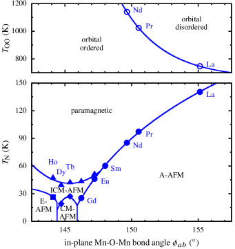
Figure 1: Phase diagram of the orbital (top) and spin (bottom) order in the early series of $R$MnO₃ as a function of the in-plane Mn-O-Mn bond angle $\phi_{ab}$. Adapted from Ref. Kimura et al. (2003)

In this study, we aim to investigate the evolution of the electronic and magnetic properties in the early series of $R$MnO₃ ($R$ = La, Pr, Nd, Sm, Eu, Gd). By combining first-principles calculations and the tight binding (TB) approach via maximally localized Wannier functions (MLWFs), we calculate the TB parameters by applying the methodology that was described in Ref. Franchini et al. (2012) for LaMnO₃. Two alternative model parameterizations are considered, which account for the effects of the electron-electron (el-el) interaction either implicitly in the otherwise non-interacting TB parameters or explicitly via a mean-field el-el interaction term in the TB Hamiltonian. Using this methodology, we explore the changes in the band structure of $R$MnO₃ and construct, compare and interpret the obtained TB parameters. Different levels of approximation to the XC kernel are adopted: standard DFT within GGA, hybrid functionals, and GW. Thereby a ready-to-use set of TB parameters is provided for future studies.

We will start with a brief overview of the basic ground state properties of the $R$MnO₃ series (Sec. II) followed by two methodological sections focused on the description of the tight-binding parametrization (Sec. III) and the ab initio calculations (Sec. IV). The results for the electronic structure, magnetic properties and tight binding parameters are presented and discussed in Sec. V. The article ends with a brief summary and conclusions.

II The $R$MnO₃ series: fundamentals

The ground state electronic structure of $R$MnO₃ ($R=$ La, Pr, Nd, Sm, Eu and Gd) is characterized by the crystal-field induced breaking of the degeneracy of the Mn³⁺ $3d^{4}$ manifold in the high-spin configuration ($t_{2g}$)³ ($e_{g}$)¹, with the $t_{2g}$ orbitals lying lower in energy than the two-fold degenerate $e_{g}$ ones. Due to the strong Hund’s rule coupling, the spins in the fully occupied majority $t_{2g}$ orbitals ${(S=3/2)}$ are aligned parallel to the spin in the singly occupied majority $e_{g}$ state ${(S=1/2)}$ at the same site. The orbital degeneracy in the $e_{g}$ channel is further lifted via cooperative Jahn-Teller distortions Rodríguez-Carvajal et al. (1998); Chatterji et al. (2003); Sánchez et al. (2003); Qiu et al. (2005), manifested by long and short Mn-O octahedral bonds alternating within the conventional orthorhombic basal plane, which are accompanied by GdFeO₃-type (GFO) checkerboard tilting and rotations of oxygen octahedra Elemans et al. (1971); Norby et al. (1995); Woodward (1997) (see Fig. 2).

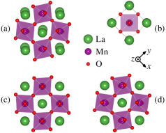
Figure 2: (a) The experimental $R$MnO₃ crystal structure (example of $R=\mathrm{La}$) with distortion modes imposed on (b) the simple cubic perovskite structure: (c) the pure JT $Q^{x}$ mode distortion and (d) the pure GFO-type distortion. Structural models were generated with VESTA Momma and Izumi (2011). Adapted from Fig. 1 in Ref. Kováčik and Ederer (2010).

As a result, the ideal cubic perovskite structure is strongly distorted into an orthorhombic structure with Pbnm symmetry Elemans et al. (1971); Norby et al. (1995) and it has been experimentally confirmed that the orbital ordering is of C-type, where the occupied $e_{g}$ orbitals follow the checkerboard JT distortion pattern in the $xy$-plane and the planes are stacked along the $z$-axis Murakami et al. (1998). The occupied $e_{g}$ orbital can be represented by a linear combination of the $d_{z^{2}}$ and $d_{x^{2}-y^{2}}$ character orbitals as ${|\theta\rangle=\mathrm{cos}\frac{\theta}{2}|3z^{2}-r^{2}\rangle+\mathrm{sin}\frac{\theta}{2}|x^{2}-y^{2}\rangle}$, where $\theta$ is the orbital mixing angle Yin et al. (2006); Kanamori (1960); Pavarini and Koch (2010); Sikora and Oleś (2003).

The most important structural characteristics as a function of the rare earth cation radius $r_{R}$ are collected in Fig. 3.

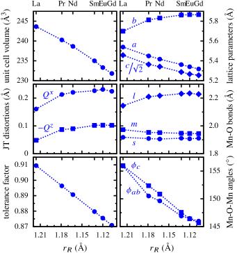
Figure 3: (color online) Dependence of various structural parameters on the $R$ cation radius $r_{R}$, taken or calculated from the experimental crystal structures at room temperature. LaMnO₃ data are taken from Ref. Norby et al. (1995), $R$MnO₃ ($R=$ Pr, Nd) from Ref. Alonso et al. (2000) and $R$MnO₃ ($R=$ Sm, Eu, Gd) from Ref. Mori et al. (2002). The tolerance factor is calculated using the ionic radii listed in Ref. Shannon (1976).

As $r_{R}$ decreases from La to Gd, the major effect is the unit cell volume $V$ reduction associated with the progressive decrease of the lattice parameters $a$ and $c$ (the so called “lanthanide contraction”). In Ref. Alonso et al. (2000), it was pointed out that the characteristic relation ${c/\sqrt{2}<a<b}$ has its origin in the strong cooperative JT effect, inducing orbital ordering and distorting the MnO₆ octahedra. The local JT distortion modes are defined as ${Q^{x}=(l-s)/\sqrt{2}}$ and ${Q^{z}=(2m-l-s)/\sqrt{6}}$, where $l$, $s$ and $m$ stand for long, short and medium Mn-O bond lengths, respectively. From the trend shown in Fig. 3, a sizable increase of both ${\lvert{Q^{z}}\rvert}$ and $Q^{x}$ can be seen in all members of the series as compared to LaMnO₃, stemming from the increase in $l$ while $m$ and $s$ remain almost unchanged.

Another important quantity in the physics of $AB$O₃ compounds is the tolerance factor $t$ Goldschmidt (1926), which gives an indication on the degree of structural distortions and the stability of the perovskite crystal structure. It can be defined as ${t=(r_{A}+r_{\mathrm{O}})/\big{[}\sqrt{2}(r_{B}+r_{\mathrm{O}})\big{]}}$, where $r_{A}$, $r_{B}$ and $r_{\mathrm{O}}$ are the ionic radii of $A$, $B$ and O, respectively. For the simple cubic perovskite structure, ${t=1}$. Depending on the magnitude of $t$, different crystal structures are formed. In $R$MnO₃, the $A=R$ cations are too small to completely fill the space in the cubic structure. In this situation, the MnO₆ octahedra undergo collective rotations to maximize the space filling, thereby reducing the Mn-O-Mn bond angles from the ideal $180^{\circ}$. Clearly, the trend of the tolerance factor $t$ is in accordance with the trend of the Mn-O-Mn bond angles. According to Zhou and Goodenough Zhou and Goodenough (2003), the transition temperature $T_{\mathrm{N}}$ depends linearly on $\langle\cos^{2}\phi\rangle$, where the average is taken over the three distinguishable Mn-O-Mn bond angles, i.e. the two $\phi_{ab}$ bond angles in the $ab$-plane and the $\phi_{c}$ bond angle in the $c$-direction.

III Methodology: Tight binding parameterization

Within the TB formalism, the effective electronic Hamiltonian of the $e_{g}$ character manifold in manganites is generally written as a sum of the following contributions: the kinetic energy term $\hat{H}_{\mathrm{kin}}$ and several local interaction terms such as the Hund’s rule coupling to the $t_{2g}$ core spin $\hat{H}_{\mathrm{Hund}}$, the JT coupling to the oxygen octahedra distortion $\hat{H}_{\mathrm{JT}}$ and the electron-electron interaction $\hat{H}_{\mathrm{el-el}}$ Ederer et al. (2007); Kováčik and Ederer (2011, 2010); Franchini et al. (2012):

$$\hat{H}_{\mathrm{kin}}= -\sum_{\begin{subarray}{c}\bm{\mathit{R}},\Delta\bm{\mathit{R}},\sigma\\ a,b\end{subarray}}\hat{c}^{\sigma\dagger}_{a\left(\bm{\mathit{R}}+\Delta\bm{\mathit{R}}\right)}t^{\sigma}_{a\left(\bm{\mathit{R}}+\Delta\bm{\mathit{R}}\right)b\left(\bm{\mathit{R}}\right)}\hat{c}^{\sigma}_{b\left(\bm{\mathit{R}}\right)}\,,$$ (1)

$$\hat{H}_{\mathrm{Hund}}= -J_{\mathrm{H}}\sum_{\begin{subarray}{c}\bm{\mathit{R}},\sigma,\sigma^{\prime}\\ a\end{subarray}}{\bm{\mathit{S_{R}}}}\hat{c}^{\sigma\dagger}_{a\left(\bm{\mathit{R}}\right)}{\bm{\tau}_{\sigma\sigma^{\prime}}}\hat{c}^{\sigma^{\prime}}_{a\left(\bm{\mathit{R}}\right)}\,,$$ (2)

$$\hat{H}_{\mathrm{JT}}= -\lambda\sum_{\begin{subarray}{c}\bm{\mathit{R}},\sigma,i\\ a,b\end{subarray}}\hat{c}^{\sigma\dagger}_{a\left(\bm{\mathit{R}}\right)}Q^{i}_{\bm{\mathit{R}}}\tau_{ab}^{i}\hat{c}^{\sigma}_{b\left(\bm{\mathit{R}}\right)}\,,$$ (3)

$$\hat{H}_{\mathrm{el-el}}= \frac{1}{2}\sum_{\begin{subarray}{c}\bm{\mathit{R}},\sigma,\sigma^{\prime}\\ a,b,c,d\end{subarray}}U_{abcd}\hat{c}^{\sigma\dagger}_{a(\bm{\mathit{R}})}\hat{c}^{\sigma^{\prime}\dagger}_{b(\bm{\mathit{R}})}\hat{c}^{\sigma^{\prime}}_{d(\bm{\mathit{R}})}\hat{c}^{\sigma}_{c(\bm{\mathit{R}})}\,.$$ (4)

The annihilation $\hat{c}^{\sigma}_{a\left(\bm{\mathit{R}}\right)}$ and the creation $\hat{c}^{\sigma\dagger}_{a\left(\bm{\mathit{R}}\right)}$ operators are associated with orbital $|{a}\rangle$ at a particular Mn site $\bm{\mathit{R}}$ (not to be confused with cation $R$) and spin $\sigma$. In the kinetic energy term, $t^{\sigma}_{a\left(\bm{\mathit{R}}+\Delta\bm{\mathit{R}}\right)b\left(\bm{\mathit{R}}\right)}$ is the hopping parameter between orbital $|{b}\rangle$ at site $\bm{\mathit{R}}$ and orbital $|{a}\rangle$ at site $\bm{\mathit{R}}+\Delta\bm{\mathit{R}}$. Further on, $J_{\mathrm{H}}$ is the Hund’s rule strength of coupling to the normalized $t_{2g}$ core spin $\bm{\mathit{S_{R}}}$, $\lambda$ is the JT coupling constant and $Q^{i}_{\bm{\mathit{R}}}$ is the amplitude of the particular JT mode $(i=\{x,z\})$ and $\tau_{ab}^{i}$ are the standard Pauli matrices. In this study, the electron-electron interaction term is treated within a mean-field approximation following the approach of Dudarev et al. Dudarev et al. (1998), involving a single parameter ${U_{\mathrm{W}}=U_{aaaa}=U_{abab}}$, with all other interaction matrix elements set to zero.

To obtain the model parameters we have extended the work presented in Ref. Franchini et al. (2012) to the $R$MnO₃ early series, wherein the model parameters are obtained from the Hamiltonian matrix elements in the MLWF basis. We will use a simplified notation for the MLWF matrix elements with the two basis functions of ${\lvert 3z^{2}-r^{2}\rangle}$ and ${\lvert x^{2}-y^{2}\rangle}$ character centered at the same site. Thereby, the MLWF matrix element $h^{\Delta\bm{\mathit{T}}}_{mn}$, where $\Delta\bm{\mathit{T}}$ is the lattice translation and $m$ and $n$ are general orbital-site indices, can be written as: $h^{\Delta\bm{\mathit{T}}}_{mn}\rightarrow h^{\Delta\bm{\mathit{T}}}_{a\bm{\mathit{R}},b\bm{\mathit{R}}^{\prime}}\rightarrow h^{\Delta\bm{\mathit{R}}}_{ab}$, where $\Delta\bm{\mathit{R}}=\bm{\mathit{R}}^{\prime}-\bm{\mathit{R}}+\Delta\bm{\mathit{T}}$. In order to disentangle the effect of the JT distortion from other lattice distortions, the TB model parameters are obtained from two crystal structures: the experimental and the purely JT $Q^{x}$ mode distorted structure, defined by the projection of the differences in the Wyckoff positions of the experimental and the simple cubic perovskite structure to the JT $Q^{x}$ mode (see Table 1). We note that in this study we use the room temperature crystal structures Norby et al. (1995); Alonso et al. (2000); Mori et al. (2002) to maintain a consistent reference for all members of the $R$ series given the available experimental data. Therefore, the results for LaMnO₃ will differ from those in Ref. Franchini et al. (2012), where the low temperature (4.2 K) structure from Ref. Elemans et al. (1971) was used in turn.

Table 1: Wyckoff positions of the $R=$ La, Pr, Nd, Sm, Eu, Gd site $(4c)$ and the two inequivalent oxygen sites O1 $(4c)$ and O2 $(8d)$ in the room temperature Pbnm experimental structures (Expt.), taken from Refs. Norby et al. (1995); Alonso et al. (2000); Mori et al. (2002) and described in Fig. 3, and their decomposition into the unit cell volume preserving structures with only the $Q^{x}$ distortion mode (JT). Mn cations are at the high symmetry site $(4b)$ with Wyckoff positions ($\nicefrac{{1}}{{2}}$, 0, 0).

		Wyckoff Positions
		Expt.	JT
LaMnO3	La	(0.9937, 0.0435, $\nicefrac{{1}}{{4}}$)	(0.0, 0.0, $\nicefrac{{1}}{{4}}$)
	O1	(0.0733, 0.4893, $\nicefrac{{1}}{{4}}$)	(0.0, 0.5, $\nicefrac{{1}}{{4}}$)
	O2	(0.7257, 0.3014, 0.0385)	(0.7635, 0.2636, 0.0)
PrMnO3	Pr	(0.9911, 0.0639, $\nicefrac{{1}}{{4}}$)	(0.0, 0.0, $\nicefrac{{1}}{{4}}$)
	O1	(0.0834, 0.4819, $\nicefrac{{1}}{{4}}$)	(0.0, 0.5, $\nicefrac{{1}}{{4}}$)
	O2	(0.7151, 0.3174, 0.0430)	(0.7662, 0.2662, 0.0)
NdMnO3	Nd	(0.9886, 0.0669, $\nicefrac{{1}}{{4}}$)	(0.0, 0.0, $\nicefrac{{1}}{{4}}$)
	O1	(0.0878, 0.4790, $\nicefrac{{1}}{{4}}$)	(0.0, 0.5, $\nicefrac{{1}}{{4}}$)
	O2	(0.7141, 0.3188, 0.0450)	(0.7664, 0.2665, 0.0)
SmMnO3	Sm	(0.9850, 0.0759, $\nicefrac{{1}}{{4}}$)	(0.0, 0.0, $\nicefrac{{1}}{{4}}$)
	O1	(0.0970, 0.4730, $\nicefrac{{1}}{{4}}$)	(0.0, 0.5, $\nicefrac{{1}}{{4}}$)
	O2	(0.7076, 0.3241, 0.0485)	(0.7659, 0.2658, 0.0)
EuMnO3	Eu	(0.9841, 0.0759, $\nicefrac{{1}}{{4}}$)	(0.0, 0.0, $\nicefrac{{1}}{{4}}$)
	O1	(0.1000, 0.4700, $\nicefrac{{1}}{{4}}$)	(0.0, 0.5, $\nicefrac{{1}}{{4}}$)
	O2	(0.7065, 0.3254, 0.0487)	(0.7660, 0.2660, 0.0)
GdMnO3	Gd	(0.9384, 0.0807, $\nicefrac{{1}}{{4}}$)	(0.0, 0.0, $\nicefrac{{1}}{{4}}$)
	O1	(0.1030, 0.4710, $\nicefrac{{1}}{{4}}$)	(0.0, 0.5, $\nicefrac{{1}}{{4}}$)
	O2	(0.7057, 0.3246, 0.0508)	(0.7651, 0.2651, 0.0)

Two types of model parameterizations are employed, namely, Model 1 and Model 2. Model 1 is an effectively "non-interacting" case, in which the $\hat{H}_{\mathrm{el-el}}$ term is neglected with the purpose of exploring how the more sophisticated beyond-PBE treatment of the XC kernel affects the hopping, JT- and GFO-distortion related parameters. Model 2 is an alternative way, involving an explicit treatment of $\hat{H}_{\mathrm{el-el}}$ in the model Hamiltonian within the mean-field approximation. This allows to obtain estimates of the corresponding on-site interaction parameter by keeping the PBE on-site model parameters as reference (see below).

In the following, for completeness, the considered TB model parameters are briefly described. For more details on the practical use of the VASP2WANNIER90 interface, as well as the derivation of the model parameters used in this study, we refer to Ref. Franchini et al. (2012).

III.1 Hopping parameters

The kinetic energy is parameterized with seven parameters: four hopping amplitudes and the JT distortion induced splitting in the nearest neighbor hopping matrix, all evaluated in the purely JT $Q^{x}$ mode distorted structure, and two spin-dependent reduction parameters of the hoppings due to the GFO distortion. For notation clarity, we set the origin ($\bm{\mathit{R}}=\mathbf{0}$) at one of the Mn sites and align the $x$ and $y$ cartesian axes with the direction of the long and short Mn-O bonds of the JT $Q^{x}$ mode, respectively. The vectors $\hat{\bm{\mathit{x}}}$, $\hat{\bm{\mathit{y}}}$, $\hat{\bm{\mathit{z}}}$ correspond to the nearest-neighbor spacing of the Mn sites along the respective axes Franchini et al. (2012).

Nearest-neighbor hopping amplitudes $t^{ss}$ between sites within the FM planes ($t^{\uparrow\uparrow}$, $t^{\downarrow\downarrow}$, $s$ is a local spin index) are obtained as ${t^{ss}=\big{(}{h_{11}^{x}}-3{h_{22}^{x}}\big{)}/2}$. The hopping parameter between sites with antiparallel spin alignment is calculated as ${t^{ss^{\prime}}=\big{(}t^{\uparrow\uparrow}+t^{\downarrow\downarrow}\big{)}/2}$. The corresponding hopping matrices are then expressed as ${{\bf{t}}^{ss^{\prime}}(\pm\hat{\bm{\mathit{z}}})=-t^{ss^{\prime}}\big{(}{\bf{I}}+{\bm{\tau}}^{z}\big{)}/2}$ and ${{\bf{t}}^{ss}(\pm\hat{\bm{\mathit{x}}})=-t^{ss}\big{(}2\,{\bf{I}}-\sqrt{3}\,{\bm{\tau}}^{x}-{\bm{\tau}}^{z}\big{)}/4}$, where $\bf{I}$ is the unity matrix. Here and in the following, the matrices along $\pm\hat{\bm{\mathit{y}}}$ are simply obtained by the relevant symmetry transformation of the matrices along $\pm\hat{\bm{\mathit{x}}}$.

The JT distortion induces a splitting between the non-diagonal elements of the nearest-neighbor hopping matrix. We model it as ${\Delta{\bf{t}}^{ss}(\pm\hat{\bm{\mathit{x}}})=\mathrm{i}\,\widetilde{\lambda}\,Q^{x}_{\bm{\mathit{R}}}{\bm{\tau}}^{y}}$, where the parameter $\widetilde{\lambda}$ is obtained as ${\widetilde{\lambda}=\sum_{s}{\big{(}h_{12}^{x}-h_{21}^{x}\big{)}^{s}}/\left(4Q^{x}\right)}$.

The second-nearest neighbor hopping $t^{xy}$ and the second-nearest neighbor hopping along the $x$, $y$, $z$ crystal axes $t^{2z}$ are obtained as ${t^{xy}=-\sum_{s}\big{(}h_{11}^{xy}\big{)}^{s}/2}$ and ${t^{2z}=-\sum_{s}\big{(}h_{11}^{2z}\big{)}^{s}/2}$. While the hopping matrices related to $t^{2z}$ have the same form as those of $t^{ss}$, the second-nearest neighbor hopping matrices are expressed via ${{\bf{t}}(\pm\hat{\bm{\mathit{x}}}\pm\hat{\bm{\mathit{z}}})=t^{xy}\big{(}{\bf{I}}-\sqrt{3}\,{\bm{\tau}}^{x}+{\bm{\tau}}^{z}\big{)}}$ and ${{\bf{t}}(\pm\hat{\bm{\mathit{x}}}\pm\hat{\bm{\mathit{y}}})=t^{xy}\big{(}{\bf{I}}-2\,{\bm{\tau}}^{z}\big{)}}$.

In GFO distorted structures, all hopping matrices are scaled by a spin-dependent reduction factor $(1-\eta_{t}^{s})$, where $\eta_{t}^{s}=1-t^{ss}_{(\textit{Pbnm})}/t^{ss}$. The hopping parameter $t^{ss}_{(\textit{Pbnm})}$ is obtained analogously to the $t^{ss}$ defined above but in the experimental crystal structure.

III.2 On-site parameters

The Hund’s rule coupling strength is calculated in the experimental Pbnm structure from the orbitally averaged spin splitting of the diagonal on-site MLWF matrix elements: ${J_{\mathrm{H}}=-\sum_{a,s}\mathrm{sgn}(s)\big{(}h_{aa}^{0}\big{)}^{s}/4}$, with ${\mathrm{sgn}(s)=+1/-1}$ for ${s=\,\uparrow/\downarrow}$.

The spin-dependent JT coupling parameter is determined from the eigenvalue splitting of the on-site MLWF matrix as ${\lambda^{s}={\Delta\varepsilon^{s}}/\left(2|{Q^{x}}|\right)}$, where $\Delta\varepsilon$ is evaluated as ${\Delta\varepsilon=\Big{[}{\big{(}h_{11}^{0}-h_{22}^{0}\big{)}^{2}+\big{(}2h_{12}^{0}\big{)}^{2}}\Big{]}^{1/2}}$ in the JT $Q^{x}$ mode distorted structure.

Similar to the hoppings, the JT coupling parameters $\lambda^{s}$ are reduced in the GFO distorted structure by a factor of ${(1-\eta_{\lambda})}$, where ${\eta_{\lambda}=1-\big{(}\Delta\varepsilon^{\uparrow}_{(\textit{Pbnm})}/\lvert{\bm{\mathit{Q}}}\rvert\big{)}/\big{(}\Delta\varepsilon^{\uparrow}/Q^{x}\big{)}}$, with ${\lvert\bm{\mathit{Q}}\rvert=\sqrt{(Q^{x})^{2}+(Q^{z})^{2}}}$.

III.3 Interaction parameters

As it was shown in Ref. Franchini et al. (2012), the $U_{\mathrm{W}}$ interaction parameter can be parameterized either by mapping the el-el interaction on the difference between the majority and minority spin on-site matrix elements and suitably introducing an appropriate correction to the JT splitting $\Delta\lambda_{\mathrm{W}}^{(J)}$, or by mapping on the splitting between the occupied and unoccupied $e_{g}$ bands with an appropriate correction to the Hund’s coupling $\Delta J_{\mathrm{W}}^{(\lambda)}$. Here, we use the latter approach, which is described as follows.

The effective Hubbard parameter $U_{\mathrm{W}}^{(\lambda)}$ in the MLWF basis is determined as a correction to the JT induced gap (controlled by $\lambda^{\uparrow}$) in the non-interacting (PBE) case. It is calculated as ${U_{\mathrm{W}}^{(\lambda)}=\big{(}\Delta\varepsilon^{\uparrow}-\Delta\varepsilon^{\uparrow}_{(\mathrm{PBE})}\big{)}/\Delta{n}^{\uparrow}}$, where $\Delta\varepsilon^{\uparrow}$ is the eigenvalue splitting of the Hamiltonian on-site matrix for a particular beyond-PBE treatment of the XC functional, $\Delta\varepsilon^{\uparrow}_{(\mathrm{PBE})}$ its corresponding value at the PBE level and $\Delta{n}^{\uparrow}$ the eigenvalue splitting of the majority occupation matrix in the MLWF basis (all evaluated in the experimental Pbnm structure). The observation that both the on-site part of the Hamiltonian and the occupation matrix can be diagonalized by the same unitary transformation was employed in the formulation.

Since the correlation-induced increase of the spin-splitting is only partially covered by the one-parameter TB el-el term $U_{\mathrm{W}}^{(\lambda)}$, it can be corrected by introducing an empirical correction to the Hund’s rule coupling: ${\Delta J_{\mathrm{W}}^{(\lambda)}=J_{\mathrm{H}}-J_{\mathrm{H(PBE)}}-U_{\mathrm{W}}^{(\lambda)}/4}$.

IV Methodology: Ab initio calculations

Spin polarized DFT calculations were performed using the Vienna ab initio simulation package (VASP) Kresse and Hafner (1993); Kresse and Furthmüller (1996), without inclusion of spin-orbit coupling. Three types of XC functional treatment were employed: (1) the standard GGA with the parameterization of Perdew-Burke-Ernzerhof (PBE)  Perdew et al. (1996); (2) the screened hybrid DFT following the recipe of Heyd, Scuseria, and Ernzerhof (HSE)  Heyd et al. (2003, 2006), involving the inclusion of 1/4 of the exact Hartree-Fock exchange in the PBE XC functional; and (3) the GW method Hedin (1965), where the XC contributions are directly accounted for from the self-energy. We have adopted a single shot G₀W₀ procedure which, at a relatively moderate computational cost, generally leads to a significant improvement of the electronic properties with respect to standard DFT and hybrid functionals. Wavefunctions of the converged PBE calculation were used as a starting point in the evaluation of the Green’s function G₀ and the fixed screened exchange W₀ Paier et al. (2008); Franchini et al. (2010).

The one-particle Kohn-Sham orbitals are computed using projected-augmented-wave (PAW) pseudopotentials Blöchl (1994); Kresse and Joubert (1999), with the rare-earth $f$ states frozen in the core (except for La). The $3s$ and $3p$ semicore states of Mn, as well as the $5s$ and $5p$ semicore states of $R$, were treated as valence, except for Eu and Gd where the $5s$ semicore states are excluded from the valence. For oxygen we have used the soft potential. Integrations in reciprocal space were carried out over a regular $\Gamma$-centered ${{6}\times{6}\times{4}}$ $k$-point mesh, except for G₀W₀ where a reduced setting of ${{4}\times{4}\times{4}}$ was adopted. The plane-wave energy cutoff was set to 400 eV for PBE and G₀W₀. After testing the influence of the energy cutoff on the HSE tight binding parameters, a value of 300 eV was used in all HSE calculations to reduce the computational cost. The total number of bands was increased to 320 in the G₀W₀ runs. This value leads to sufficiently well converged band gap (within 0.1-0.2 eV) but a larger value would be needed to better describe the highest unoccupied $e_{g}$ manifold. Unfortunately, the inclusion of a larger number of bands would result in a prohibitive computational cost.

Ground state electronic, optical and magnetic properties were calculated for the experimental Pbnm structure in the A-AFM order. By mapping the total energy differences among different magnetic configurations to the Heisenberg Hamiltonian, exchange coupling parameters were evaluated within the HSE approach. With the so determined exchange parameters, an estimate for the Néel temperature was computed via Monte Carlo simulations (MC), employing the Metropolis algorithm Metropolis et al. (1953) and using the Mersenne twister for the random number generation Matsumoto and Nishimura (1998). Finally, the TB parameters were extracted from the Hamiltonian matrix elements in the basis of the MLWFs, constructed from the ab initio wavefunctions in the A-AFM experimental and $Q^{x}$ mode JT structures with the VASP2WANNIER90 interface Franchini et al. (2012). For practical reasons, the $f$ states of La were pushed away from the Mn $e_{g}$ energy window in the PBE calculations by applying $U=10$ eV, following the recipe of Dudarev et al. Dudarev et al. (1998).

V Results and discussion

In this section we present the outcomes of the combined ab initio and model Hamiltonian analysis. First we discuss the ground state electronic structure, MLWFs and dielectric properties as derived from the ab initio PBE, HSE and G₀W₀ calculations. Then we will focus on the detailed explanation of the origin of the A-type AFM ordering by mapping the HSE total energies onto a Heisenberg Hamiltonian and computing the ordering temperature $T_{\text{N}}$ from Monte Carlo simulations. Finally, an extended section will be dedicated to the TB results.

V.1 Electronic and dielectric properties

Figure 4 (a), (b) and (c) depict the calculated band structures at the PBE, HSE and G₀W₀ level, respectively, for $R$MnO₃ ($R=$ La, Pr, Nd, Sm, Eu and Gd) along with the corresponding characteristic MLWFs bands of predominantly $e_{g}$ character.

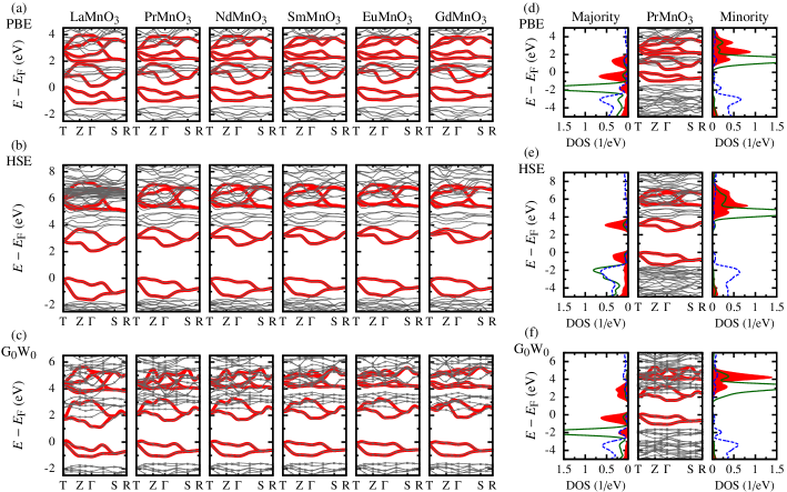
Figure 4: (color online) The ab initio (thin lines) and $e_{g}$ character MLWF (thick lines) band structure of $R$MnO₃ ($R=$ La, Pr, Nd, Sm, Eu, Gd); for (a) PBE (b) HSE and (c) G₀W₀. Band structure and associated normalized projected density of states (PDOS) for PrMnO₃: Mn $e_{g}$ (filled areas under curve), Mn $t_{2g}$ (solid lines) and O $p$ (dashed line) for (d) PBE (e) HSE and (f) G₀W₀. Left/right PDOS correspond to local majority/minority Mn sites while O $p$ PDOS is calculated as an average over all O sites.

It is seen that upon $R$ substitution, the features of the $e_{g}$ character bands do not exhibit substantial differences. Consequently, the electronic properties, including screening effects, could be expected to remain almost unchanged over the series. The band structures depict an insulating state with an indirect energy gap. As a representative example of all compounds in the series, we show in Figs. 4(d)-(f) the band structure and associated projected density of states (PDOS) of PrMnO₃. The PDOS is shown for the Mn $e_{g}$/$t_{2g}$ and O $p$ character. The overall bonding picture resembles closely the one of LaMnO₃ Franchini et al. (2012); He and Franchini (2012); He et al. (2012): the indirect band gap is opened between the lower laying $e_{g}$ states, there is a strong hybridization between Mn $d$ and O $p$ states, and an appreciable intermixing between Mn $e_{g}$ and $t_{2g}$ states is observed, in particular around the band gap.

The band gaps of $R$MnO₃ and the local magnetic moments at the Mn³⁺ sites with the different levels of exchange-correlation treatment are presented in Tab. 2.

Table 2: The values of indirect (smallest direct) band gap and magnetic moment at the Mn³⁺ sites of $R$MnO₃ series.

	Band gap (eV)
	PBE	HSE	G0W0	Expt.
LaMnO3	0.13 (0.56)	2.06 (2.48)	1.15 (1.49)	1.7${}^{\text{a}}$, 1.9${}^{\text{b}}$, 2.0${}^{\text{c}}$
PrMnO3	0.32 (0.72)	2.43 (2.74)	1.63 (1.81)	1.75${}^{\text{d}}$, 2.0${}^{\text{e}}$
NdMnO3	0.36 (0.74)	2.49 (2.78)	1.70 (1.86)	1.75${}^{\text{d}}$, 1.78${}^{\text{f}}$
SmMnO3	0.40 (0.75)	2.61 (2.80)	1.79 (1.92)	1.82${}^{\text{f}}$
EuMnO3	0.42 (0.75)	2.65 (2.85)	1.84 (1.96)
GdMnO3	0.45 (0.75)	2.70 (2.89)	1.87 (1.99)	2.0${}^{\text{g}}$, 2.9${}^{\text{h}}$
	Magnetic moment ($\mu_{B}$)
	PBE	HSE	G0W0	Expt.
LaMnO3	3.49	3.72	3.40	3.4${}^{\text{i}}$, 3.87${}^{\text{j}}$, 3.65${}^{\text{k}}$
PrMnO3	3.49	3.71	3.40	3.5${}^{\text{l}}$
NdMnO3	3.49	3.71	3.40	3.22${}^{\text{m}}$
SmMnO3	3.49	3.71	3.40	3.3${}^{\text{n}}$
EuMnO3	3.49	3.71	3.40
GdMnO3	3.47	3.70	3.38

${}^{\text{a\,}}$Ref. Saitoh et al. (1995); ${}^{\text{b\,}}$Ref. Jung et al. (1997); ${}^{\text{c\,}}$Ref. Krüger et al. (2004); ${}^{\text{d\,}}$Ref. Kim et al. (2006); ${}^{\text{e\,}}$Ref. Sopracase et al. (2006); ${}^{\text{f\,}}$Ref. Shetkar and Salker (2010); ${}^{\text{g\,}}$Ref. Wang et al. (2010); ${}^{\text{h\,}}$Ref. Negi et al. (2013); ${}^{\text{i}}\,$Ref. Hauback et al. (1996); ${}^{\text{j}}\,$Ref. Moussa et al. (1996); ${}^{\text{k}}\,$Ref. Huang et al. (1997); ${}^{\text{l}}\,$Ref. Laverdière et al. (2006); ${}^{\text{m}}\,$Ref. Muñoz et al. (2000); ${}^{\text{n}}\,$Ref. O’Flynn et al. (2011).

The magnetic moment at the Mn³⁺ sites remains basically unaltered along the $R$ series, while a general trend of the band gap increase from La to Gd is seen at all XC levels. The overall increment in the direct band gap is of about 0.4 and 0.5 eV at the HSE and G₀W₀ level, respectively, and in the indirect band gap of about 0.7 eV in both cases. The experimental data, not available for EuMnO₃, do not show a clear trend but are generally in line with the G₀W₀ expectations for the direct band gap. Although still capturing the insulating nature, PBE results in much too small values of the band gap as expected. On the other hand, the HSE values appear too overestimated. This is likely due to the amount of exact exchange incorporated in the HSE functional. In the present study, we have used the standard 0.25 compromise Heyd et al. (2003, 2006). However, recent systematic studies on the role of the mixing parameter on the physical properties of perovskites have indicated that a lower fraction should be used (0.1-0.15), to achieve a more consistent picture He and Franchini (2012); Franchini (2014).

The dielectric function measured in an energy range between 0.5 to 5.5 eV shows two intensive, broad optical features peaked at approximately 2 eV and 4.5 eV for LaMnO₃ (Fig. 5).

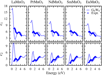
Figure 5: (color online) The real ($\epsilon_{1}$) and imaginary ($\epsilon_{2}$) part of the dielectric function. The dotted lines indicate the G₀W₀ data and the filled diamonds correspond to the experimental data taken from Ref. Moskvin et al. (2010).

For the other $R$MnO₃ compounds, the intensive broad peak is positioned at $\approx{2.2}$ eV. While the authors in Refs. Ahn and Millis (2000); Kovaleva et al. (2004) assign the peaks to ${d\hbox{-}d}$ charge transfer excitations, the authors of Ref. Moskvin et al. (2010) argue that the peaks are due to the interplay of both ${p\hbox{-}d}$ and ${d\hbox{-}d}$ transitions. These experimental results are in line with the measurements of Kim et al. Kim and Min (2009). The G₀W₀ results capture well the double peak structure, but the intensity of the first peak and the zero frequency value of the real part of the dielectric function $\epsilon_{1}$, which identifies the macroscopic dielectric constant $\epsilon_{\infty}$, is about two times larger than the experimental one. A better agreement with experiment could possibly be achieved by increasing the number of bands, the $k$-points sampling and by treating the screened exchange at beyond-PBE level (i.e., within a fully self-consistent GW framework) but this is beyond the scope of the present study (the corresponding calculation would be computationally very demanding) He and Franchini (2014) and will be addressed in a future article Ergonenc et al. (In preparation).

V.2 Magnetic properties

We further analyze the magnetic properties of the $R$MnO₃ compounds in terms of the exchange interactions $J_{ij}$ between sites $i$ and $j$, obtained by mapping the total energy of different magnetic configurations on the Heisenberg Hamiltonian

$$H=-\frac{1}{2}\sum_{i\neq j}J_{ij}\,\bm{\mathit{S}}_{i}\cdot\bm{\mathit{S}}_{j},$$ (5)

for ${\lvert{\bm{\mathit{S}}_{i}}\rvert=\lvert{\bm{\mathit{S}}_{j}}\rvert=2}$, with positive and negative values of $J_{ij}$ corresponding to FM and AFM coupling, respectively. In the four formula unit cell there are three exchange interactions that can be extracted: the in-plane nearest neighbor $J_{x}$, the out-of-plane nearest neighbor $J_{z}$ and second nearest neighbor $J_{xz}$; where the subscripts are a shorthand notation of the direction connecting the sites in the pseudo-cubic axes frame [see Fig. 6(a)]. Determining interactions between further neighbors would require a larger supercell. While often only the first two parameters are taken into consideration Muñoz et al. (2004); Evarestov et al. (2005), it was reported that the A-AFM order in LaMnO₃ can be seen as a competition between a weakly FM $J_{z}$ and a weakly AFM $J_{xz}$ coupling Solovyev et al. (1996). As it was discussed previously, simple treatments of the exchange-correlation functional (such as PBE) were shown to be inadequate in providing a good prediction of the magnetic properties/interactions for perovskites and in general for transition metal oxides Yamauchi et al. (2008); Archer et al. (2011). Although the exchange interactions in LaMnO₃ calculated using hybrid functionals were found to be largely dependent on the choice of the particular hybrid functional, the A-AFM order is consistently predicted to be the magnetic ground state Muñoz et al. (2004). We therefore base our analysis on the total energies calculated using the HSE functional, that has been already employed successfully in combination with the Monte Carlo method to predict the magnetic ordering temperature in transition metal perovskites Franchini et al. (2011).

We also note that a recent study has shown that the magnetic properties of the later members of the manganite series ($R=$ Tb to Lu) are not well described by a standard Heisenberg model with pairwise bilinear interactions, and that additional biquadratic or four-spin ring exchange interactions need to be considered Fedorova et al. (2015). However, for the larger rare earth cations considered in this study, the Heisenberg model is expected to provide a sufficiently accurate description.

The total energy was calculated for the five symmetry inequivalent magnetic configurations compatible with the unit cell. These include: the ferromagnetic order (B); the three distinct antiferromagnetic configurations A-AFM (A), C-AFM (C) and G-AFM (G); and the single non-degenerate ferrimagnetic state (Fi), as depicted in Fig. 6(a).

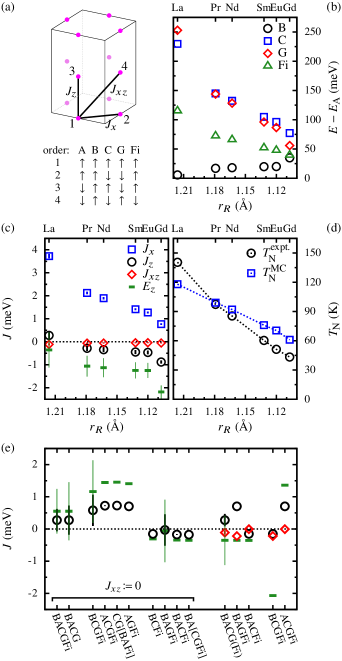
Figure 6: (color online) (a) Schematic representation of the exchange interactions $J_{x}$, $J_{z}$ and $J_{xz}$ in the unit cell of $R$MnO₃, together with the spin orientations in the A, B, C, G and Fi magnetic configurations. (b) The total energy of the different magnetic configurations relative to the A ordering. (c) Exchange interactions calculated by linear least-square fit of Eqs. (6a) to (6e) and the out-of-plane interlayer interaction energy $E_{z}=2J_{z}+8J_{xz}$. Errors on the estimation of the corresponding parameter are shown as vertical bars. (d) The Néel temperature, experimental $T_{\text{N}}^{\text{expt.}}$ Kimura et al. (2003) and calculated $T_{\text{N}}^{\text{MC}}$ via MC simulations using the exchange interactions shown in (c). (e) $J_{z}$, $J_{xz}$ and $E_{z}$ in LaMnO₃ for different sets of magnetic configurations. For sets yielding identical values of $J_{z}$, we adopt a notation of choose one from the list in square brackets. The BACG(Fi) data depicts both BACGFi (with error bars) and BACG (without error bars). Legend is identical to (c).

For brevity, the shorthand notation in parentheses Wollan and Koehler (1955) will be used in this section to denote the total energies of the corresponding magnetic configuration. These, by using Eq. (5), are expressed as:

$$E_{\text{A}} = E_{0}-32J_{x}+16J_{z}+64J_{xz},$$ (6a)

$$E_{\text{B}} = E_{0}-32J_{x}-16J_{z}-64J_{xz},$$ (6b)

$$E_{\text{C}} = E_{0}+32J_{x}-16J_{z}+64J_{xz},$$ (6c)

$$E_{\text{G}} = E_{0}+32J_{x}+16J_{z}-64J_{xz},$$ (6d)

$$E_{\text{Fi}} = E_{0}.$$ (6e)

where $E_{0}$ is a fitting constant in unit of energy that should correspond to the energy of the paramagnetic state. The total energies relative to $E_{\text{A}}$ are plotted in Fig. 6(b). For all members of the $R$ series, the A ordering yields the lowest energy among the five considered magnetic configurations. While the difference in the total energy from the C or G orders on one side to the A or B orders on the other side are relatively large in case of LaMnO₃, these differences decrease consistently towards GdMnO₃, following the trend of decreasing $T_{\text{N}}$. We note that $(E_{\text{C}}-E_{\text{A}})$ does not differ from $2(E_{\text{Fi}}-E_{\text{A}})$ by more than 2 meV.

The solution to the overdetermined system of equations composed by Eqs. (6a) to (6e) is obtained by linear least-squares fit and the resulting exchange interaction parameters $J_{x}$, $J_{z}$ and $J_{xz}$ are shown in Fig. 6(c). The in-plane $J_{x}$ interaction is FM throughout the whole $R$ series, monotonously and strongly decreasing from La to Gd. The out-of-plane $J_{z}$ interaction exhibits a similar trend, however, the weakly FM $J_{z}$ for $R=$ La becomes weakly AFM from $R=$ Pr on. The stability of A order is finally determined by the out-of-plane interaction energy $E_{z}=2J_{z}+8J_{xz}$ being negative for all members of $R$ series, including La. There, however, the error on the estimation of $E_{z}$ is large enough to reach the FM region. By employing the Monte Carlo method, the exchange interaction parameters are used to calculate the Néel temperature presented in Fig. 6(d), generally leading to very good agreement with the experimental values Kimura et al. (2003).

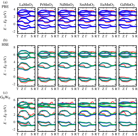
Figure 7: (color online) The TB bands calculated according to Model 1 (filled circles) and Model 2 (crosses) with the MLWFs bands (solid lines) in the background.

We note that for the case of LaMnO₃ it is of particular importance to include the out-of-plane second neighbor interaction in the model. Furthermore, the calculated exchange interactions are particularly sensitive to the choice of the subset $M$ of magnetic configurations to include in the system of equations [see Fig. 6(e)]. By setting $J_{xz}=0$ and operating Eqs. (6a) to (6e), it is easy to show that $J_{z}$ can be calculated from any of the following expressions:

$$(E_{\text{A}}+E_{\text{G}}-2E_{\text{Fi}}) :\quad \{\text{AGFi}\}\in M$$ (7a)

$$(2E_{\text{Fi}}-E_{\text{B}}-E_{\text{C}}) :\quad \{\text{BCFi}\}\in M$$ (7b)

$$(E_{\text{A}}-E_{\text{B}}) :\quad \{\text{AB}\}\in M$$ (7c)

$$(E_{\text{G}}-E_{\text{C}}) :\quad \{\text{CG}\}\in M.$$ (7d)

For $R=$ Pr to Gd, the $J_{z}$ calculated from Eqs. (7a) to (7d) is always negative, whereas in LaMnO₃ its sign becomes positive when using Eqs. (7a) and (7d). Using all five energy points (BACGFi) the linear least-squares fit to Eqs. (6a) to (6e) yields a FM $J_{z}$ whose magnitude is the average obtained from Eqs. (7a) and (7b), but with an error in the estimation of the parameter large enough to turn it AFM. An out-of-plane FM coupling is obtained when either AGFi or CG are present in $M$, which is inconsistent with the experimentally observed magnetic ground state (sets BCGFi, ACGFi, BCG, ACG, CGFi and AGFi). Conversely, when either BCFi or AB are present in $M$ (sets BCFi, BAGFi, BACFi, BAC, BAG, and BAFi), the system of equations yields a negative $J_{z}$ in agreement with experiments. However, that would be the equivalent of removing inconvenient data to adjust it to a desired outcome, when actually these inconsistencies can be ascribed to the fact that without $J_{xz}$ the expansion of the Heisenberg Hamiltonian is incomplete. Including $J_{xz}$ as a third interaction parameter, only Eqs. (7a) and (7b) hold. The out-of-plane magnetic coupling is driven by the previously defined interaction energy $E_{z}$, which can be regarded as the effective out-of-plane exchange interaction. As shown in Fig. 6(e), provided that both A and B are present in $M$, $E_{z}$ is not only negative but rather insensitive to the configuration of the subset, in spite of the pronounced differences obtained in the particular values of $J_{z}$ and $J_{xz}$. This is so because $E_{z}$ is calculated as

$$(E_{\text{A}}-E_{\text{B}}) \!\!\!\!\!\!:\ \ \{\text{AB}\}\in M$$ (8a)

$$(4E_{\text{Fi}}-2E_{\text{B}}-E_{\text{C}}-E_{\text{G}}) \!\!\!\!\!\!:\ \ \text{A}\notin M$$ (8b)

$$(2E_{\text{A}}+E_{\text{C}}+E_{\text{G}}-4E_{\text{Fi}}) \!\!\!\!\!\!:\ \ \text{B}\notin M.$$ (8c)

When either A or B are not members of $M$, Eqs. (8b) and (8c) would be equivalent to Eq. (8a) if the following identity, stemming from Eqs. (6a) to (6e), is verified: $E_{\text{A}}+E_{\text{B}}+E_{\text{C}}+E_{\text{G}}=4E_{\text{Fi}}$. However, not only the Heisenberg model is itself an approximation but also the ab initio total energies are not exempt from errors due to various approximations affecting the calculations. Since the out-of-plane exchange parameters are of comparable magnitude to these errors (in the order of meV), minor deviations in the previous equality lead to the observed large differences in $J_{z}$, $J_{xz}$ and $E_{z}$. This is the reason why it is advisable and often necessary to extract the exchange parameters from as large sets of magnetic configurations as possible.

V.3 Tight binding

We remind that we performed two types of TB parameterization: Model 1 and Model 2. In Model 1, the term $\hat{H}_{\mathrm{el-el}}$ is not considered, the el-el interaction is implicitly accounted for in the HSE and G₀W₀ hopping, JT- and GFO-induced parameters, which will differ from the corresponding PBE values. In Model 2, the modifications due to the beyond-PBE methods are treated as a perturbation to the “noninteracting” PBE description by explicitly considering the $\hat{H}_{\mathrm{el-el}}$ term in the mean-field approximation. The band structures obtained with these sets of TB parameters compared with the corresponding MLWFs bands are shown in Fig. 7. The individual TB parameters are shown in Figs. 8 and 9 and are presented in detail in Tab. 3.

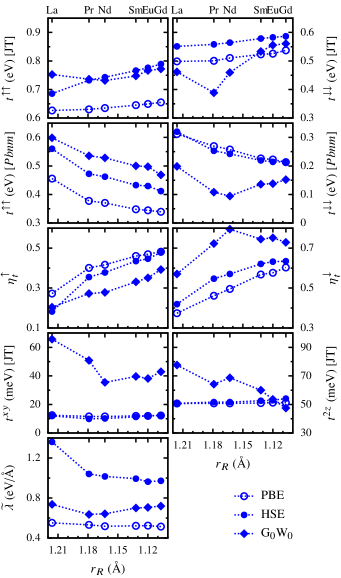
Figure 8: Dependence of the TB hopping related model parameters on $r_{R}$. The nearest neighbor hopping parameters $t^{\uparrow\uparrow}$ and $t^{\downarrow\downarrow}$ are shown in the JT($Q^{x}$) and experimental Pbnm crystal structure, which are used to determine the GFO-induced reduction factors $\eta^{\uparrow}$ and $\eta^{\downarrow}$. As next, the further neighbor hopping parameters $t^{xy}$ and $t^{2z}$ and the JT-induced splitting in the non-diagonal elements of the nearest neighbor in-plane hopping matrix $\widetilde{\lambda}$ are shown.

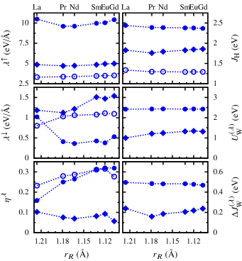
Figure 9: Dependence of the TB on-site model parameters on $r_{R}$: JT coupling parameters $\lambda^{\uparrow}$, $\lambda^{\downarrow}$ and the GFO-induced reduction parameter of the JT coupling $\eta^{\lambda}$, Hund’s coupling $J_{\mathrm{H}}$, the mean-field Hubbard parameter $U_{\mathrm{W}}^{(\lambda)}$ and the correction to the Hund’s coupling $\Delta{J}_{W}^{(\lambda)}$. For legend see Fig. 8.

In general, very good qualitative agreement can be seen between the features of the TB and MLWF bands (Fig. 7). Moreover, almost no difference is found between the bands calculated with the TB parameters using Model 1 and Model 2. While the match for LaMnO₃ at PBE level (for which the procedure was originally developed in Ref. Kováčik and Ederer (2010)) is very good, deviations for the lowest unoccupied $e_{g}$ character band increase along the $R$ series. This is not surprising considering that the progressively stronger GFO distortion makes the assumption of the individual structural distortions acting independently less valid. Nevertheless, the root mean square and maximum deviation between the band and $k$-point averaged sets of eigenvalues for the TB and MLWF bands are typically around very acceptable values: 0.15 and 0.5 eV, respectively. The quantitative deviations observed in the G₀W₀ local minority bands can be, on the other hand, attributed to difficulties in achieving well-converged results at the G₀W₀ level.

In the following we analyze in detail how the hopping and on-site TB parameters are affected along the $R$ series at different levels of the XC functional treatment.

Table 3: The tight binding parameters. The hopping parameters $t^{\uparrow\uparrow}$ and $t^{\downarrow\downarrow}$ for the JT structure in Fig. 8 correspond to the $t^{\uparrow\uparrow}$ and $t^{\downarrow\downarrow}$ presented in this table.

			Hopping parameters								On-site parameters					Model 2
			$t^{\uparrow\uparrow}$	$t^{\downarrow\downarrow}$	$\widetilde{\lambda}$	$t^{xy}$	$t^{2z}$	$\eta_{t}^{\uparrow}$	$\eta_{t}^{\downarrow}$		$J_{\mathrm{H}}$	$\lambda^{\uparrow}$	$\lambda^{\downarrow}$	$\eta_{\lambda}$		$\Delta\varepsilon^{\uparrow}$	$\Delta{n}^{\uparrow}$	$U_{\mathrm{W}}^{(\lambda)}$	$\Delta{J}_{\mathrm{W}}^{(\lambda)}$
			(meV)	(meV)	(eV/Å)	(meV)	(meV)				(eV)	(eV/Å)	(eV/Å)			(eV)		(eV)	(eV)
PBE	LaMnO3		627	499	0.55	12	51	0.27	0.37		1.34	3.31	0.80	0.23		0.85
	PrMnO3		631	500	0.53	12	51	0.40	0.46		1.30	3.36	1.03	0.28		1.12
	NdMnO3		635	511	0.52	12	51	0.42	0.50		1.30	3.39	1.06	0.29		1.15
	SmMnO3		645	523	0.52	12	51	0.46	0.57		1.29	3.46	1.08	0.31		1.18
	EuMnO3		649	526	0.52	12	51	0.47	0.58		1.29	3.49	1.11	0.31		1.21
	GdMnO3		655	537	0.51	12	51	0.48	0.60		1.29	3.52	1.10	0.28		1.26
HSE	LaMnO3		686	551	1.36	12	51	0.18	0.42		2.44	10.49	1.02	0.16		2.96	0.87	2.42	0.50
	PrMnO3		732	558	1.04	10	52	0.35	0.55		2.39	9.59	0.41	0.25		3.31	0.90	2.43	0.48
	NdMnO3		743	564	1.02	10	52	0.38	0.57		2.39	9.61	0.36	0.26		3.36	0.91	2.44	0.48
	SmMnO3		766	579	0.99	11	53	0.44	0.62		2.38	9.97	0.43	0.31		3.41	0.92	2.42	0.48
	EuMnO3		776	583	0.96	12	53	0.45	0.63		2.38	10.03	0.38	0.32		3.45	0.92	2.43	0.48
	GdMnO3		789	587	0.97	12	54	0.48	0.63		2.37	10.41	0.53	0.32		3.50	0.93	2.43	0.47
G0W0	LaMnO3		753	462	0.74	66	78	0.20	0.57		1.83	4.86	1.18	0.10		1.46	0.61	1.00	0.24
	PrMnO3		736	389	0.64	51	64	0.27	0.72		1.76	4.71	1.12	0.08		2.00	0.73	1.21	0.16
	NdMnO3		732	460	0.64	36	69	0.28	0.79		1.79	4.73	1.22	0.07		2.10	0.76	1.24	0.19
	SmMnO3		747	533	0.70	40	60	0.33	0.74		1.83	4.85	1.51	0.08		2.21	0.78	1.32	0.21
	EuMnO3		767	556	0.71	38	54	0.35	0.75		1.85	4.95	1.47	0.09		2.27	0.79	1.35	0.22
	GdMnO3		772	561	0.72	43	48	0.39	0.73		1.86	4.99	1.54	0.06		2.32	0.81	1.32	0.24

Regarding the hopping parameters [Fig. 8 and Tab. 3], the nearest neighbor hoppings $t^{\uparrow\uparrow}$ and $t^{\downarrow\downarrow}$ (calculated using the purely JT distorted structure) exhibit a slight monotonic increase with $R$ for PBE and HSE, which can be attributed to the unit cell volume reduction. This trend is not followed for early $R$ series members at G₀W₀. The deviation is not as pronounced for $t^{\uparrow\uparrow}$ as it is for $t^{\downarrow\downarrow}$, but in general, as mentioned above, results for the minority bands at G₀W₀ should be taken with much care. The increase in $t^{\uparrow\uparrow}$ from the PBE values to those at beyond PBE levels is due to the stronger hybridization with lower lying O $p$ states Kováčik and Ederer (2011); Franchini et al. (2012). The strong reduction of the hopping amplitude due to the increasing GFO distortion along the $R$ series can be seen in the plots of $t^{\uparrow\uparrow}$ and $t^{\downarrow\downarrow}$ (calculated using the Pbnm structure) and in the corresponding derived reduction parameters $\eta_{t}^{\uparrow}$ and $\eta_{t}^{\downarrow}$. While the reduction is strongest at PBE, generally followed by HSE and G₀W₀ in the case of majority spin, reversed behavior can be seen for the minority spin. The decrease of the hoppings correlates with the reduction of Mn-O-Mn in-plane angle $\phi_{ab}$ and the Néel temperature. The further neighbor hopping parameters $t^{xy}$ and $t^{2z}$ remain nearly unchanged along the $R$ series for PBE and HSE. Not much significance should be given to the irregularities observed for G₀W₀, since the notorious difficulty to properly converge the minority bands can have a very pronounced effect on these parameters. The $\widetilde{\lambda}$ parameter, controlling the JT induced splitting in the hopping matrix, is largely independent on $R$ (except $R=\text{La}$ for HSE) and its magnitude increases from PBE through G₀W₀ to HSE, resembling the behavior of the on-site parameters $\lambda^{\uparrow}$ and $J_{\mathrm{H}}$ (see below).

The on-site TB parameters as a function of $R$ calculated for different XC kernel treatment are presented in Fig. 9 and Tab. 3. For completeness, the numerical values of the majority spin eigenvalue splitting $\Delta\varepsilon^{\uparrow}$ and occupation matrix splitting $\Delta{n}^{\uparrow}$ needed for $U_{\mathrm{W}}^{(\lambda)}$ evaluation are also listed in Tab. 3. The majority spin JT coupling strength $\lambda^{\uparrow}$ and the Hund’s rule coupling strength $J_{\mathrm{H}}$ are almost constant along the $R$ series. They also exhibit a mutually consistent qualitative increase at the HSE and G₀W₀ levels (compare with $\widetilde{\lambda}$ above), which is reflected in the TB model by an increase in the band gap ($\lambda^{\uparrow}$) and the spin splitting ($J_{\mathrm{H}}$). The magnitude of $\lambda^{\downarrow}$ is significantly smaller than that of $\lambda^{\uparrow}$. This can be explained using the simple argument of the weaker $d$-$p$ hybridization for the higher lying minority bands Kováčik and Ederer (2010). The irregularities along the $R$ series for G₀W₀ are again caused by the quality of the minority spin bands. The reduction parameter of the JT coupling strength due to the GFO distortion $\eta^{\lambda}$ is weaker than the corresponding hopping reduction parameters ($\eta^{\uparrow}$ and $\eta^{\downarrow}$). Its relative change down the $R$ series is comparable for PBE and HSE, while the results for G₀W₀ are almost $R$ independent.

In order to capture both the spin splitting and the band gap increase when using HSE and G₀W₀, a single interaction parameter $U_{\mathrm{W}}^{(\lambda)}$ is not sufficient and a semi-empirical correction to the Hund’s coupling $\Delta{J}_{\mathrm{W}}^{(\lambda)}$ is also needed in Model 2. Here, the hopping parameters of the respective method are used, while the on-site parameters are kept fixed at their PBE values. The el-el interaction parameter $U_{\mathrm{W}}^{(\lambda)}$ as a function of $R$ can be regarded as a constant for HSE, while it exhibits a small increase in the case of G₀W₀. The value of $U_{\mathrm{W}}^{(\lambda)}$ is significantly different for HSE and G₀W₀. The much larger HSE value can be a consequence of the mixing parameter used in these calculations He and Franchini (2012); Franchini (2014), which consistently leads to an overestimation of the band gap (see Table 2). The quantitatively less important $\Delta{J}_{\mathrm{W}}^{(\lambda)}$ follows the same trend as $U_{\mathrm{W}}^{(\lambda)}$.

VI Conclusions

A combination of first-principles calculations and tight-binding (TB) model Hamiltonian via Maximally localized Wannier functions (MLWFs) was applied to the parent compounds of manganites $R$MnO₃ ($R$ = La, Pr, Nd, Sm, Eu and Gd). The electronic and magnetic properties were studied at different levels of XC treatment.

The band structures within the same XC level exhibit similar features along the $R$ series. The calculations show a clear trend of an increase of the electronic band gap with the decrease of the $R$ cation radius $r_{R}$. While PBE band gaps are severely underestimated, the HSE values are overestimated likely due to the amount of the exact exchange included in the functional. The values obtained for G₀W₀ seem to be more consistent with the available experimental data. Likewise, the dielectric function calculated within G₀W₀ is in reasonable qualitative agreement with experiments but the intensity of the first peak and $\epsilon_{\infty}$ are significantly overestimated.

The exchange couplings obtained at the HSE level yield Monte Carlo simulated Néel temperatures that are in very good agreement with experimental observations. The weakening of the FM in-plane exchange interaction parameter with decreasing $r_{R}$ is a clear indication of the destabilization of the A-type AFM order towards the E-type AFM order observed in further members of the $R$ series. Concurrently, the effective AFM out-of-plane exchange interaction strengthens and it is only in LaMnO₃ where the out-of-plane antiferromagnetism can not be attributed to a single exchange parameter.

Despite the difficulties in the disentanglement of the $e_{g}$ character states mainly at the G₀W₀ level, the obtained MLWF bands are in very good agreement with the underlying ab initio bands. The method-derived changes in the TB parameters due to different treatments of the XC kernel has been investigated and accounted for using two parameterization models. In general, an overall consistent qualitative trend in the description of the TB parameters has been found for all the compounds down the $R$ series at the PBE, HSE and G₀W₀ levels. The trends in the nearest neighbor hopping amplitudes in the Pbnm structure are comparable with those of the volume, tolerance factor, Mn-O-Mn bond angles and the Néel temperature. Another interesting result is that the JT and Hund’s rule coupling strength, as well as the simple mean-field electron-electron interaction parameter, are practically $R$ independent and can be regarded as method dependent universal constants in the $R$MnO₃ series.