Multi-soliton, multi-breather and higher order rogue wave solutions to the complex short pulse equation

Abstract

In the present paper, we are concerned with the general localized solutions for the complex short pulse equation including soliton, breather and rogue wave solutions. With the aid of a generalized Darboux transformation, we construct the $N$-bright soliton solution in a compact determinant form, then the $N$-breather solution including the Akhmediev breather and a general higher order rogue wave solution. The first- and second-order rogue wave solutions are given explicitly and illustrated by graphs. The asymptotic analysis is performed rigourously for both the $N$-soliton and the $N$-breather solutions. All three forms of the localized solutions admit either smoothed-, cusped- or looped-type ones for the CSP equation depending on the parameters. It is noted that, due to the reciprocal (hodograph) transformation, the rogue wave solution to the CSP equation is different from the one to the nonlinear Schrödinger (NLS) equation, which could be a cusponed- or a looped one.
Keywords: Complex short pulse equation, Darboux transformation, bright soliton, breather soliton, rogue wave, asymptotic analysis
Mathematics Subject Classification: 39A10, 35Q58

I Introduction

The nonlinear Schrödinger (NLS) equation, as one of the universal models that describe the evolution of slowly varying packets of quasi-monochromatic waves in weakly nonlinear dispersive media, plays an key role in nonlinear optics Hasegawa ; Agrawal . Recently, there are several experiments reported related to the modulational instability (MI) and the breather solution MI ; Zakh of the NLS equation in nonlinear optics. The Akhmediev breather (periodic in space but localized in time) AB , the Peregrine soliton or rogue wave (RW) solution (time and space homoclinic) Pregr and the Kuznetsov-Ma soliton (periodic in time but localized in space) K-M have recently been experimentally observed in optical fibers Dudley ; Kibler ; Kibler1 in succession. Beside the experimental observation in optical fibers, the RWs have also been observed in water-wave tanks Chabchoub and plasmas Bailung .

However, in the regime of ultra-short pulses where the width of optical pulse is in the order of femtosecond ($10^{-15}$ s), the quasi-monochromatic assumption to derive the NLS equation is not valid anymore Roth . Description of ultra-short processes requires a modification of standard slow varying envelope models based on the NLS equation. There are usually two ways to satisfy this requirement in the literature. The first one is to add several higher-order dispersive terms to yield higher-order NLS equation Agrawal . The second one is to construct a suitable fit to the frequency-dependent dielectric constant $\varepsilon(\omega)$ in the desired spectral range. Several models have been proposed by the latter approach such as the short-pulse (SP) equation Sch ; Sko ; Kim ; Amir and the complex short pulse (CSP) equation Feng2 .

Recently, Schäfer and Wayne derived a short pulse (SP) equation Sch

$$u_{xt}=u+\frac{1}{6}(u^{3})_{xx}$$ (1)

to describe the propagation of ultra-short optical pulses in nonlinear media. Here, $u=u(x,t)$ is a real-valued function, representing the magnitude of the electric field. The SP equation (1) has been shown to be completely integrable Robelo ; Beals ; Sako ; Brun ; Brun1 . The periodic and soliton solutions of the SP equation (1) were found in Sako1 ; Kuet ; Parkes . The connection between the SP equation (1) and the sine-Gordon equation through the reciprocal transformation was clarified, and then the $N$-soliton solutions including multi-loop and multi-breather ones were given in Matsuno ; Matsuno1 by using the Hirota’s bilinear method Hirota . The integrable discretization and the geometric interpretation of the SP equation were given in Feng ; Feng1 .

Most recently, one of the authors proposed a complex short pulse (CSP) equation Feng2

$$q_{xt}+q+\frac{1}{2}(|q|^{2}q_{x})_{x}=0$$ (2)

that governs the propagation of ultra short pulse packet along optical fibers. There are several advantages in using complex representation description of wave phenomenon, especially of the optical waves Yariv . Firstly, amplitude and phase are two fundamental characteristics for a wave packet, the information of these two factors are nicely combined into a single complex-valued function. Secondly, the use of complex representation can make a lot of manipulations including soliton interactions much easier. Such advantages can be observed in many analytical results related to the NLS equation, the complex short pulse equation and their coupled models. As is shown in Feng2 ; shen , in contrast with the fact that one-soliton solution to the SP equation is always a loop soliton without physical meaning (1), the one-soliton solution to the CSP equation (2) is an envelope soliton with a few optical cycles.

Compared to the SP equation, few results are known to the CSP equation (2). It is necessary to study the CSP equation mathematically, as well as its applications in nonlinear optics. Therefore, it is the aim of the present paper to investigate all kinds of solutions of the CSP equation by Darboux transformation.

Based on the previous study Feng2 ; shen , it is known that the CSP equation (2) is linked to a complex coupled dispersionless (CCD) equation cd

$$\begin{split}&q_{ys}=\rho q,\\ &\rho_{s}+\frac{1}{2}(|q|^{2})_{y}=0,\end{split}$$ (3)

through the following reciprocal (hodograph) transformation

$$\mathrm{d}x=\rho\mathrm{d}y-\frac{1}{2}|q|^{2}\mathrm{d}s,\,\,\mathrm{d}t=-\mathrm{d}s,$$ (4)

The CCD equation (3) is the first negative flow of the Landau-Lifshitz hierarchy，while the SP and the CSP equations being the first negative flow of Wadati-Konno-Ichikawa (WKI) hierarchy WKI ; Qiao ; Zimerman . By constructing a generalized Darboux transformation to the CCD equation and integrating the integrals exactly involved in the reciprocal (hodograph) transformation, we are able to construct the general analytical solutions to the CSP equation including the $N$-bright soliton, $N$-breather solution and higher order rogue wave solutions.

It should be pointed out that the compact formulas for these solutions are more convenient for us to perform the asymptotic analysis. Recently the modulational instability has been also considered as a wave breaking mechanism breaking . Indeed, if the initial steepness of the monochromatic wave is large, during the process of modulational instability, one wave will start growing and will soon reach the limiting steepness, and break before becoming a rogue wave. The NLS theory does not predict the breaking or overturning of the waves Onorato . Different from previous research regarding the rogue wave solution to the NLS equation, we find that there exists the wave breaking phenomenon in the rogue wave theory of the CSP equation (2). These results could deepen our understanding about the MI mechanism Zakharov .

The outline of the present paper is organized as follows. In section II, the generalized Darboux transformation Matveev ; Guo1 ; Guo2 of the CCD equation was derived through loop group method loop-group . Based on the generalized Darboux transformation, we can obtain the general soliton formulas for the CCD equation. Further, by integrating the reciprocal transformation exactly, we can construct the general soliton formulas for the CSP equation. In section III, the $N$-bright soliton solution and the $N$-breather solution are constructed, and their asymptotic analyses are performed. In section IV, we construct the rogue wave solution including the first-order and general higher order rogue wave solution. Section IV is devoted to conclusions and some discussions. In Appendices, we give the details involving the proofs of asymptotic analysis and the modulational instability analysis.

II Generalized Darboux transformation for the CSP equation

Prior to giving the Darboux transformation (DT) for the CSP equation (2), we briefly review the link between the CSP equation and the CCD equation. It is known that the CCD equation (3) admits the following Lax pair

$$\begin{split}\Psi_{y}=&U(\rho,q;\lambda)\Psi,\\ \Psi_{s}=&V(q;\lambda)\Psi,\end{split}$$ (5)

where

$$U(\rho,q;\lambda)=\begin{bmatrix}-\frac{\mathrm{i}\rho}{\lambda}&-\frac{q_{y}^{\ast}}{\lambda}\\[8.0pt] \frac{q_{y}}{\lambda}&\frac{\mathrm{i}\rho}{\lambda}\end{bmatrix},\,\,V(q;\lambda)=\left(\frac{\mathrm{i}}{4}\lambda\sigma_{3}+\frac{\mathrm{i}}{2}Q\right),\,\,\sigma_{3}=\mathrm{diag}(1,-1),\,\,Q=\begin{bmatrix}0\,&\,q^{\ast}\\[8.0pt] q\,&\,0\end{bmatrix}\,,$$ (6)

and ^∗ represents the complex conjugate. Through the reciprocal transformation (4), one can obtain the CSP equation (2) and its Lax pair:

$$\begin{split}\Psi_{x}=&\begin{bmatrix}-\frac{\mathrm{i}}{\lambda}&-\frac{q_{x}^{\ast}}{\lambda}\\[8.0pt] \frac{q_{x}}{\lambda}&\frac{\mathrm{i}}{\lambda}\end{bmatrix}\Psi,\\ \Psi_{t}=&\begin{bmatrix}-\frac{\mathrm{i}}{4}\lambda+\frac{\mathrm{i}|q|^{2}}{2\lambda}&-\frac{\mathrm{i}q^{\ast}}{2}+\frac{|q|^{2}q_{x}^{\ast}}{2\lambda}\\[8.0pt] -\frac{\mathrm{i}q}{2}-\frac{|q|^{2}q_{x}}{2\lambda}&\frac{\mathrm{i}}{4}\lambda-\frac{\mathrm{i}|q|^{2}}{2\lambda}\end{bmatrix}\Psi.\end{split}$$ (7)

On the contrary, the CSP equation (2) can be transformed into the CCD equation (3). Note that the CSP equation (2) can be rewritten as the following conservative form

$$\left(\sqrt{1+|q_{x}|^{2}}\right)_{t}+\frac{1}{2}\left(|q|^{2}\sqrt{1+|q_{x}|^{2}}\right)_{x}=0\,,$$ (8)

thus, by letting $\rho^{-1}=\sqrt{1+|q_{x}|^{2}}$ and defining an inverse reciprocal transformation

$$\mathrm{d}y=\rho^{-1}\mathrm{d}x-\frac{1}{2}\rho^{-1}|q|^{2}\mathrm{d}t,\,\,\mathrm{d}s=-\mathrm{d}t,$$ (9)

we can convert system (7) into system (5). The equivalence between the CSP and the CCD equations is kind of formal under the reciprocal and inverse reciprocal transformations. The rigorous equivalence is valid only if $\rho\neq 0$ for $(y,s)\in\mathbb{R}^{2},$ or $|u_{x}|\neq\infty$ for $(x,t)\in\mathbb{R}^{2}.$

To construct the soliton and rogue wave solutions for the CSP equation (2), we give the following proposition

Proposition 1

The Darboux matrix

$$T=I+\frac{\lambda_{1}^{\ast}-\lambda_{1}}{\lambda-\lambda_{1}^{\ast}}P_{1},\,\,P_{1}=\frac{|y_{1}\rangle\langle y_{1}|}{\langle y_{1}|y_{1}\rangle},\langle y_{1}|=|y_{1}\rangle^{{\dagger}},\,\,|y_{1}\rangle=\begin{bmatrix}\psi_{1}(y,s;\lambda_{1})\\ \phi_{1}(y,s;\lambda_{1})\\ \end{bmatrix}$$ (10)

where $|y_{1}\rangle$ is a special solution for linear system (5) with $\lambda=\lambda_{1}$, can convert system (5) into a new system

$$\begin{split}\Psi[1]_{y}=&U(\rho[1],q[1];\lambda)\Psi[1],\\ \Psi[1]_{s}=&V(\rho[1],q[1];\lambda)\Psi[1].\end{split}$$ (11)

The Bäcklund transformations between $(\rho[1],q[1])$ and $(\rho,q)$ are given through

$$\begin{split}\rho[1]=&\rho-2\ln_{ys}\left(\frac{\langle y_{1}|y_{1}\rangle}{\lambda_{1}^{\ast}-\lambda_{1}}\right),\\ q[1]=&q+\frac{(\lambda_{1}^{\ast}-\lambda_{1})\psi_{1}^{\ast}\phi_{1}}{\langle y_{1}|y_{1}\rangle},\\ |q[1]|^{2}=&|q|^{2}+4\ln_{ss}\left(\frac{\langle y_{1}|y_{1}\rangle}{\lambda_{1}^{\ast}-\lambda_{1}}\right).\end{split}$$ (12)

Proof: The Darboux transformation for the system (5) is a standard one for the AKNS system with $SU(2)$ symmetry. The rest of the proposition is to prove the formulas (12), in which carry on some ideas from the classical monograph algebraic .

Suppose there is a holomorphic solution for Lax pair equation (5) in some punctured neighborhood of infinity on the Riemann surface, smoothing depending on $y$ and $s$. Thus, we may assume the following asymptotical expansion as $\lambda\rightarrow\infty.$

$$\begin{bmatrix}\psi_{1}\\ \phi_{1}\end{bmatrix}=\left[\begin{bmatrix}1\\ 0\end{bmatrix}+\sum_{i=1}^{\infty}\Psi_{i}\lambda^{-i}\right]\exp{\left(\frac{\mathrm{i}}{4}\lambda s\right)}\,,$$ (13)

for the wave function $\Psi$ and

$$T=I+\sum_{i=1}^{\infty}T^{[i]}\lambda^{-i}.$$ (14)

for the Darboux matrix $T$. Since $T$ is the Darboux matrix, it satisfies the following relations

$$T_{y}+TU=U[1]T.$$ (15)

By comparing the entries of the matrices, we get

$$\begin{split}q_{y}[1]&=q_{y}+\left(T_{2,1}^{[1]}\right)_{y},\\ \rho[1]&=\rho+\mathrm{i}\left(T_{1,1}^{[1]}\right)_{y}\,.\end{split}$$ (16)

Integrating the first equation with respect to $y$, we have the second equation in (12). Let

$$H\equiv q^{\ast}\frac{\phi_{1}}{\psi_{1}}=\sum_{i=1}^{\infty}H_{i}\lambda^{-i},$$

we then have

$$(\ln H)_{s}=\frac{\phi_{1,s}}{\phi_{1}}-\frac{\psi_{1,s}}{\psi_{1}}+(\ln q^{\ast})_{s}=-\frac{\mathrm{i}}{2}\lambda-\frac{\mathrm{i}}{2}H+\frac{\mathrm{i}}{2}|q|^{2}H^{-1}+(\ln q^{\ast})_{s}$$

from the first equation of (5). Thus

$$H_{s}=\frac{\mathrm{i}}{2}|q|^{2}-\frac{\mathrm{i}}{2}\lambda H-\frac{\mathrm{i}}{2}H^{2}+(\ln q^{\ast})_{s}H.$$

Then the coefficient $H_{i}$ can be determined as following:

$$\begin{split}H_{1}=&|q|^{2},\,\,H_{2}=2\mathrm{i}q_{s}q^{\ast},\\ H_{i+1}=&2\mathrm{i}q^{\ast}\left(\frac{H_{i}}{q^{\ast}}\right)_{s}-\sum_{j=1}^{i-1}H_{j}H_{i-j},\,\,i\geq 2.\end{split}$$

On the one hand, the first equation of (5) can be rewritten as

$$\psi_{1,s}=\left(\frac{\mathrm{i}}{4}\lambda+\frac{\mathrm{i}}{2}\sum_{i=1}^{\infty}H_{i}\lambda^{-i}\right)\psi_{1}.$$

Substituting the asymptotical expansion (13)

$$\psi_{1}=\left(1+\sum_{i=1}^{\infty}\Psi_{i}^{[1]}\lambda^{-i}\right)\exp{\left(\frac{\mathrm{i}}{4}\lambda s\right)},$$

into above equation, where superscript ^[1] represents the first component of the vector, we then have

$$\Psi_{1,s}^{[1]}=\frac{\mathrm{i}}{2}H_{1}=\frac{\mathrm{i}}{2}|q|^{2}.$$ (17)

Similarly, by assuming an asymptotical expansion

$$\begin{bmatrix}\psi_{1}[1]\\ \phi_{1}[1]\\ \end{bmatrix}=\left[\begin{bmatrix}1\\ 0\\ \end{bmatrix}+\sum_{i=1}^{\infty}\Psi[1]_{i}\lambda^{-i}\right]\exp{\left(\frac{\mathrm{i}}{4}\lambda s\right)},\,\,\lambda\rightarrow\infty\,,$$ (18)

we have

$$\Psi[1]_{1,s}^{[1]}=\frac{\mathrm{i}}{2}|q[1]|^{2}.$$ (19)

Moreover, by Darboux transformation

$$\begin{bmatrix}\psi_{1}[1]\\ \phi_{1}[1]\\ \end{bmatrix}=\left(I+\sum_{i=1}^{\infty}T^{[i]}\lambda^{-i}\right)\left[\begin{bmatrix}1\\ 0\\ \end{bmatrix}+\sum_{i=1}^{\infty}\Psi_{i}\lambda^{-i}\right]\exp{\left(\frac{\mathrm{i}}{4}\lambda s\right)},$$

one can obtain

$$\left(T_{1,1}^{[1]}\right)_{s}+\Psi_{1,s}^{[1]}=\frac{\mathrm{i}}{2}|q[1]|^{2},$$ (20)

where the element $T_{i,j}^{[1]}$ denotes the $(i,j)$-th entry of matrix $T^{[1]}.$ Together with (17), we can obtain that

$$|q[1]|^{2}=|q|^{2}-2\mathrm{i}\left(T_{1,1}^{[1]}\right)_{s}.$$ (21)

Next, we proceed to the calculation of $\left(T_{1,1}^{[1]}\right)_{s}$ and $\left(T_{1,1}^{[1]}\right)_{y}$. Since

$$|y_{1}\rangle_{s}=\left(\frac{\mathrm{i}}{4}\lambda_{1}\sigma_{3}+\frac{\mathrm{i}}{2}Q\right)|y_{1}\rangle,\,\,-\langle y_{1}|_{s}\sigma_{3}=\langle y_{1}|\sigma_{3}\left(\frac{\mathrm{i}}{4}\lambda^{*}_{1}\sigma_{3}+\frac{\mathrm{i}}{2}Q\right),$$

which originates from the Lax pair of the CSP equation (2), we then have

$$\left(\frac{\langle y_{1}|y_{1}\rangle}{\lambda_{1}^{\ast}-\lambda_{1}}\right)_{s}=\frac{\mathrm{i}}{4}(-|\psi_{1}|^{2}+|\phi_{1}|^{2}).$$ (22)

On the other hand,

$$\langle y_{1}|y_{1}\rangle=|\psi_{1}|^{2}+|\phi_{1}|^{2},$$

which implies

$$\left(\frac{|\psi_{1}|^{2}}{\langle y_{1}|\sigma_{3}|y_{1}\rangle}\right)_{y}=-\left(\frac{|\phi_{1}|^{2}}{\langle y_{1}|\sigma_{3}|y_{1}\rangle}\right)_{y}.$$

Thus, we have

$$(T_{1,1}^{[1]})_{y} = \left(\frac{|\psi_{1}|^{2}}{{\displaystyle\frac{\langle y_{1}|y_{1}\rangle}{\lambda_{1}^{\ast}-\lambda_{1}}}}\right)_{y}=\left(\frac{|\psi_{1}|^{2}-|\phi_{1}|^{2}}{{\displaystyle 2\frac{\langle y_{1}|y_{1}\rangle}{\lambda_{1}^{\ast}-\lambda_{1}}}}\right)_{y}=2\mathrm{i}\ln_{ys}\left(\frac{\langle y_{1}|y_{1}\rangle}{\lambda_{1}^{\ast}-\lambda_{1}}\right).$$

Similarly, we could derive

$$(T_{1,1}^{[1]})_{s}=2\mathrm{i}\ln_{ss}\left(\frac{\langle y_{1}|y_{1}\rangle}{\lambda_{1}^{\ast}-\lambda_{1}}\right).$$ (23)

Finally, combining Eqs. (21) and (16), we obtain the last two formulas in (12). This completes the proof. $\square$

To construct a general Darboux matrix, the following identities will be used. Suppose $M$ is a $N\times N$ matrix, $\phi$, $\psi$ are $1\times N$ column vectors, then we have the following identities

$$\begin{split}&\phi M^{-1}\psi^{{\dagger}}=\frac{\begin{vmatrix}M&\psi^{{\dagger}}\\ -\phi&0\end{vmatrix}}{|M|},\\ &1+\phi M^{-1}\psi^{{\dagger}}=\frac{\begin{vmatrix}M&\psi^{{\dagger}}\\ -\phi&1\end{vmatrix}}{|M|}=\frac{\det(M+\psi^{{\dagger}}\phi)}{\det(M)},\end{split}$$ (24)

where ^† represents the Hermite conjugate. Then we have the following proposition gives the N-fold Darboux transformation and the generalized N-fold Darboux transformation for the CSP equation

Proposition 2

The N-fold Darboux transformation for the CCD equation can be represented as

$$T_{N}=I+YM^{-1}D^{-1}Y^{{\dagger}},$$ (25)

where $Y=\left[|y_{1}\rangle,|y_{2}\rangle,\cdots,|y_{N}\rangle\right],$ and

$$M=\left(\frac{\langle y_{i}|y_{j}\rangle}{\lambda_{i}^{\ast}-\lambda_{j}}\right)_{1\leq i,j\leq N},\,\,D=\mathrm{diag}\left(\lambda-\lambda_{1}^{\ast},\lambda-\lambda_{2}^{\ast},\cdots,\lambda-\lambda_{N}^{\ast}\right).$$

Moreover, the general Darboux matrix is

$$T_{N}=I+YM^{-1}D^{-1}Y^{{\dagger}},$$ (26)

where

$$\begin{split}Y=&\left[|y_{1}^{[0]}\rangle,|y_{1}^{[1]}\rangle,\cdots,|y_{1}^{[n_{1}-1]}\rangle,\cdots,|y_{r}^{[0]}\rangle,|y_{r}^{[1]}\rangle,\cdots,|y_{r}^{[n_{r}-1]}\rangle\right],\\ M=&\begin{bmatrix}M_{11}&M_{12}&\cdots&M_{1r}\\ M_{21}&M_{22}&\cdots&M_{2r}\\ \vdots&\vdots&\ddots&\vdots\\ M_{21}&M_{22}&\cdots&M_{2r}\end{bmatrix},\,\,M_{ij}=\begin{bmatrix}M_{ij}^{[1,1]}&M_{ij}^{[1,2]}&\cdots&M_{ij}^{[1,n_{j}]}\\ M_{ij}^{[2,1]}&M_{ij}^{[2,2]}&\cdots&M_{ij}^{[2,n_{j}]}\\ \vdots&\vdots&\ddots&\vdots\\ M_{ij}^{[n_{i},1]}&M_{ij}^{[n_{i},2]}&\cdots&M_{ij}^{[n_{i},n_{j}]}\end{bmatrix},\\ D=&\mathrm{diag}\left(D_{1},D_{2}\cdots,D_{r}\right),\,\,D_{i}=\begin{bmatrix}D_{i}^{[0]}&\cdots&D_{i}^{[n_{i}-1]}\\ 0&\ddots&\vdots\\ 0&0&D_{i}^{[0]}\end{bmatrix}\end{split}$$

and

$$\begin{split}|y_{i}(\lambda_{i}+\alpha_{i}\epsilon_{i})\rangle=&\sum_{k=0}^{n_{i}-1}|y_{i}^{[k]}\rangle\epsilon_{i}^{k}+O(\epsilon_{i}^{n_{i}}),\,\,\frac{1}{\lambda-\lambda_{i}^{\ast}-\alpha_{i}\epsilon_{i}^{\ast}}=\sum_{k=0}^{n_{i}-1}D_{i}^{[k]}\epsilon_{i}^{\ast k}+O(\epsilon_{i}^{\ast n_{i}})\\ \frac{\langle y_{i}(\lambda_{i}+\alpha_{i}\epsilon_{i})|y_{j}(\lambda_{j}+\alpha_{j}\epsilon_{j})\rangle}{\lambda_{i}^{\ast}-\lambda_{j}+\alpha_{i}^{\ast}\epsilon_{i}^{\ast}-\alpha_{j}\epsilon_{j}}=&\sum_{k=1}^{n_{i}}\sum_{l=1}^{n_{j}}M_{ij}^{[k,l]}\epsilon_{i}^{\ast k}\epsilon_{j}^{l}+O(\epsilon_{i}^{\ast n_{i}},\epsilon_{j}^{n_{j}}).\end{split}$$

The general Bäcklund transformations are

$$\begin{split}\rho[N]=&\rho-2\ln_{ys}(\det(M)),\\ q[N]=&q+\frac{\det(G)}{\det(M)},\\ |q[N]|^{2}=&|q|^{2}+4\ln_{ss}(\det(M))\end{split}$$ (27)

where $G=\begin{bmatrix}M&Y_{1}^{{\dagger}}\\ -Y_{2}&0\end{bmatrix}$, $Y_{k}$ represents the $k$-th row of matrix $Y$.

Proof: Through the standard iterated step for DT Guo2 , we can obtain the $N$-fold DT. Next, by using the following equalities

$$\begin{split}(T_{1,1}^{[1]})_{y}&=\left(Y_{1}M^{-1}Y_{1}^{{\dagger}}\right)_{y}=\left(-Y_{2}M^{-1}Y_{2}^{{\dagger}}\right)_{y}=\left(\frac{Y_{1}M^{-1}Y_{1}^{{\dagger}}-Y_{2}M^{-1}Y_{2}^{{\dagger}}}{2}\right)_{y}=2\mathrm{i}\ln_{ys}\left(\det(M)\right),\\ (T_{1,1}^{[1]})_{s}&=2\mathrm{i}\ln_{ss}\left(\det(M)\right),\end{split}$$

we can obtain the formula (27) from the above $N$-fold DT (25). To complete the generalized DT, we set

$$\begin{split}\lambda_{r+1}&=\lambda_{1}+\alpha_{1}\varepsilon_{1,1},\,|y_{r+1}\rangle=|y_{1}(\lambda_{r+1})\rangle;\,\,\cdots;\lambda_{r+n_{1}-1}=\lambda_{1}+\alpha_{1}\varepsilon_{1,n_{1}-1},\,|y_{r+n_{1}-1}\rangle=|y_{1}(\lambda_{r+n_{1}-1})\rangle;\\ \lambda_{r+n_{1}}&=\lambda_{2}+\alpha_{2}\varepsilon_{2,1},\;|y_{r+n_{1}}\rangle=|y_{2}(\lambda_{r+n_{1}})\rangle;\,\,\cdots,\lambda_{r+n_{1}+n_{2}-2}=\lambda_{2}+\alpha_{2}\varepsilon_{2,n_{2}-1},\,|y_{r+n_{1}+n_{2}-2}\rangle=|y_{2}(\lambda_{r+n_{1}+n_{2}-2})\rangle;\\ &\vdots\\ \lambda_{N-n_{r}+1}&=\lambda_{r}+\alpha_{r}\varepsilon_{r,1},\,|y_{N-n_{r}+1}\rangle=|y_{r}(\lambda_{N-n_{r}+1})\rangle;\,\,\cdots;\lambda_{N}=\lambda_{r}+\alpha_{r}\varepsilon_{r,n_{r}-1},\,|y_{N}\rangle=|y_{r}(\lambda_{N})\rangle.\\ &\end{split}$$

Taking limit $\varepsilon_{i,j}\rightarrow 0$, we can obtain the generalized DT (26) and formulas (27). $\square$

Recently the generalized DT for the AB system without the first and third relation in (27) was given in ref wangxin in a different form. Actually, the first and third relation in (27) are the key procedures to construct the exact solution for the CSP equation. In summary, with the aid of reciprocal transformation (4), we obtain the general expression for $N$-soliton solution of the CSP equation (2):

$$\begin{split}q[N]=&q+\frac{\det(G)}{\det(M)},\\ x=&\int\rho(y,s)\mathrm{d}y-\frac{1}{2}\int|q(y,s)|^{2}\mathrm{d}s-2\ln_{s}(\det(M)),\,\ t=-s.\end{split}$$ (28)

III Multi-soliton and Multi-breather solutions to the CSP equation

In this section, we provide multi-soliton and multi-breather solutions to the CSP equation by using formula (28).

III.1 Single soliton solution and $N$-soliton solution

We start with a seed solution

$$\rho[0]=-\frac{\gamma}{2},\,\,q[0]=0,\,\,\gamma>0.$$ (29)

Solving the Lax pair equation (5) with $(\rho,q;\lambda)=(\rho[0],q[0];\lambda_{i})$, we arrive at

$$\Psi_{i}=\begin{bmatrix}\mathrm{e}^{\theta_{i}}\\ \mathrm{e}^{-\theta_{i}}\\ \end{bmatrix},\,\,\theta_{i}=\frac{\mathrm{i}\gamma}{2\lambda_{i}}y+\frac{\mathrm{i}\lambda_{i}}{4}s+a_{i},$$ (30)

from which, we can obtain the single soliton solution through the formula (28):

$$\begin{split}q[1]=&\lambda_{1,I}\mathrm{sech}(2\theta_{1,R})\mathrm{e}^{-2\mathrm{i}\theta_{1,I}-\frac{\pi\mathrm{i}}{2}},\\ x=&-\frac{\gamma}{2}y+\lambda_{1,I}\tanh(2\theta_{1,R}),\,\,t=-s,\end{split}$$ (31)

where $\lambda_{1}=\lambda_{1,R}+{\rm i}\lambda_{1,I}$, $\theta_{1}=\theta_{1,R}+\mathrm{i}\theta_{1,I}$. We comment here that $\lambda_{1}$ is the reciprocal of the wave number $p_{1}$ in Feng1 . As discussed in Feng1 , if $\lambda_{1,R}^{2}>\lambda_{1,I}^{2}$, one has the smooth soliton solution; if $\lambda_{1,R}^{2}=\lambda_{1,I}^{2}$, ones has the cusponed soliton solution; if $\lambda_{1,R}^{2}<\lambda_{1,I}^{2}$, one obtains the loop soliton solution.

Furthermore, by using the $N$-fold DT, we could drive the $N$-soliton solution through the formula (28):

$$\begin{split}q[N]&=\frac{\det(G)}{\det(M)},\\ x&=-\frac{\gamma}{2}y-2\ln_{s}(\det(M)),\,\,\,t=-s,\end{split}$$ (32)

where

$$\begin{split}M&=\left(\frac{\mathrm{e}^{\theta_{i}^{\ast}+\theta_{j}}+\mathrm{e}^{-\theta_{i}^{\ast}-\theta_{j}}}{\lambda_{i}^{\ast}-\lambda_{j}}\right)_{1\leq i,j\leq N},\quad\,G=\begin{bmatrix}M&Y_{1}^{{\dagger}}\\ -Y_{2}&0\end{bmatrix},\\ Y_{1}&=\begin{bmatrix}\mathrm{e}^{\theta_{1}},&\mathrm{e}^{\theta_{2}},&\cdots,&\mathrm{e}^{\theta_{N}}\end{bmatrix},\quad\,Y_{2}=\begin{bmatrix}\mathrm{e}^{-\theta_{1}},&\mathrm{e}^{-\theta_{2}},&\cdots,&\mathrm{e}^{-\theta_{N}}\end{bmatrix},\end{split}$$ (33)

the expressions $\theta_{i}$’s are given in (30). The dynamics for two soliton is shown in ref. Feng2 . It should be pointed out that the interaction of two smooth solitons could yield the singularity. The condition to avoid singularity for multi-soliton can not obtained through an analytical way. Finally, to understand the dynamics of above $N$-soliton solution (32), we give the following asymptotic analysis and its proof

Proposition 3

Suppose $0<v_{1}<v_{2}<\cdots<v_{N}$. When $s\rightarrow\pm\infty$, we have

$$q[N]=\sum_{k=1}^{N}\lambda_{k,I}\mathrm{sech}(2\theta_{k,R}^{\pm})\mathrm{e}^{-2\mathrm{i}\theta_{k,I}^{\pm}-\frac{\pi\mathrm{i}}{2}}+O(\mathrm{e}^{-c|s|}),$$ (34)

where

$$\begin{split}\theta_{k,R}^{\pm}=&\frac{\gamma\lambda_{k,I}}{2|\lambda_{k}|^{2}}(y-v_{k}s)+a_{k,R}\pm\Delta_{k,R}^{\pm},\,\,\Delta_{k,R}^{\pm}=\frac{1}{2}\left(\sum_{l=1}^{k-1}\left|\frac{\lambda_{l}^{\ast}-\lambda_{k}}{\lambda_{l}-\lambda_{k}}\right|-\sum_{l=k+1}^{N}\left|\frac{\lambda_{l}^{\ast}-\lambda_{k}}{\lambda_{l}-\lambda_{k}}\right|\right),\\ \theta_{k,I}^{\pm}=&\frac{\gamma\lambda_{k,R}}{2|\lambda_{k}|^{2}}y+\frac{\lambda_{k,R}}{4}s+a_{k,I}\mp\Delta_{k,I}^{\pm},\,\,\Delta_{k,I}^{\pm}=\frac{1}{2}\left(\sum_{l=1}^{k-1}\arg\left(\frac{\lambda_{l}-\lambda_{k}}{\lambda_{l}^{\ast}-\lambda_{k}}\right)-\sum_{l=k+1}^{N}\arg\left(\frac{\lambda_{l}-\lambda_{k}}{\lambda_{l}^{\ast}-\lambda_{k}}\right)\right),\end{split}$$ (35)

and $c=\mathrm{min}\left(\left|\frac{\gamma\lambda_{k,I}}{2|\lambda_{k}|^{2}}\right|\right)\mathrm{min}_{i\neq j}(|v_{i}-v_{j}|),$ $v_{i}=\frac{|\lambda_{i}|^{2}}{2\gamma}.$

The proof is given in Appendix A. Next we analyze the coordinates transformation: as $s\rightarrow\pm\infty$, along the line $\theta_{k,R}^{\pm}=0$, we have

$$x=-\frac{\gamma}{2}y-2\ln_{s}(M)\rightarrow-\frac{\gamma}{2}y\pm\left[\sum_{i=1}^{k-1}\lambda_{i,I}-\sum_{j=k+1}^{N}\lambda_{j,I}\right],$$

it follows that

Proposition 4

When $t\rightarrow\mp\infty$, along the trajectory $\theta_{k,R}^{\pm}=0$, we have

$$q[N]=\sum_{k=1}^{N}\lambda_{k,I}\mathrm{sech}(2\theta_{k,R}^{\pm})\mathrm{e}^{-2\mathrm{i}\theta_{k,I}^{\pm}-\frac{\pi\mathrm{i}}{2}}+O(\mathrm{e}^{-c|t|}),$$

where

$$\begin{split}\theta_{k,R}^{\pm}=&-\frac{\lambda_{k,I}}{|\lambda_{k}|^{2}}x+\frac{\lambda_{k,I}}{4}t+a_{k,R}\pm\frac{\lambda_{k,I}}{|\lambda_{k}|^{2}}\left(\sum_{i=1}^{k-1}\lambda_{i,I}-\sum_{j=k+1}^{N}\lambda_{j,I}\right)\pm\Delta_{k,R}^{\pm},\\ \theta_{k,I}^{\pm}=&-\frac{\lambda_{k,R}}{|\lambda_{k}|^{2}}x-\frac{\lambda_{k,R}}{4}t+a_{k,I}\pm\frac{\lambda_{k,I}}{|\lambda_{k}|^{2}}\left(\sum_{i=1}^{k-1}\lambda_{i,I}-\sum_{j=k+1}^{N}\lambda_{j,I}\right)\mp\Delta_{k,I}^{\pm}.\end{split}$$

III.2 Single breather and multi-breather solutions

To find a single breather solution, we depart from a seed solution

$$\rho[0]=-\frac{\gamma}{2},\,\,q[0]=\frac{\beta}{2}\mathrm{e}^{\mathrm{i}\theta},\,\,\theta=y+\frac{\gamma}{2}s,\,\,\gamma>0,\,\,\beta\geq 0.$$ (36)

Then we have the solution for the Lax pair equation (5) with $(q,\rho;\lambda)=(q[0],\rho[0];\lambda_{i})$,

$$|y_{i}\rangle=KL_{i}E_{i},\,\,K=\mathrm{diag}\left(\mathrm{e}^{-\frac{\mathrm{i}}{2}\theta},\mathrm{e}^{\frac{\mathrm{i}}{2}\theta}\right),\,\,\lambda_{i}\neq-\gamma+\mathrm{i}\beta,$$ (37)

where

$$L_{i}=\begin{bmatrix}1&1\\[10.0pt] {\displaystyle\frac{\beta}{\gamma+\xi_{i}}}&{\displaystyle\frac{\beta}{\gamma+\chi_{i}}}\end{bmatrix},\,\,E_{i}=\begin{bmatrix}\mathrm{e}^{\theta_{i}}\\ \mathrm{e}^{-\theta_{i}}\end{bmatrix}$$

and

$$\begin{split}\theta_{i}=&\frac{\mathrm{i}}{4}\sqrt{\beta^{2}+(\lambda_{i}+\gamma)^{2}}\left(s+\frac{2}{\lambda_{i}}y\right)+a_{i},\\ \xi_{i}=&\lambda_{i}+\sqrt{\beta^{2}+(\lambda_{i}+\gamma)^{2}},\,\,\chi_{i}=\lambda_{i}-\sqrt{\beta^{2}+(\lambda_{i}+\gamma)^{2}}.\end{split}$$

To avoid the inconvenience of involving the square root of a complex number, we introduce the following transformation:

$$\lambda_{i}+\gamma=\beta\sinh(\varphi_{i,R}+\mathrm{i}\varphi_{i,I}),\,\,(\varphi_{i,R},\varphi_{i,I})\in\Omega,$$

where $\Omega=\{(\varphi_{R},\varphi_{I})|0<\varphi_{I}<\pi,\,\text{and }0<\varphi_{R}<\infty,\text{or }\varphi_{R}=0,\text{and }\frac{\pi}{2}\leq\varphi_{I}<\pi\}$, then

$$\xi_{i}+\gamma=\beta\mathrm{e}^{\varphi_{i,R}+\mathrm{i}\varphi_{i,I}},\,\,\chi_{i}+\gamma=-\beta\mathrm{e}^{-\varphi_{i,R}-\mathrm{i}\varphi_{i,I}}.$$

By some tedious calculations, the single breather solution can be constructed from the formula (28) by using the technique Ling

$$\begin{split}q[1]=&\frac{\beta}{2}\left[\frac{\cosh(2\theta_{1,R}-2\mathrm{i}\varphi_{1,I})\cosh(\varphi_{1,R})+\sin(2\theta_{1,I}+2\mathrm{i}\varphi_{1,R})\sin(\varphi_{1,I})}{\cosh(2\theta_{1,R})\cosh(\varphi_{1,R})-\sin(2\theta_{1,I})\sin(\varphi_{1,I})}\right]\mathrm{e}^{\mathrm{i}\theta}\,,\\ x=&-\frac{\gamma}{2}y-\frac{\beta^{2}}{8}s-2\ln_{s}\left[\cosh(2\theta_{1,R})\cosh(\varphi_{1,R})-\sin(2\theta_{1,I})\sin(\varphi_{1,I})\right],\,\,t=-s,\end{split}$$ (38)

where

$$\begin{split}\theta_{1,R}&=\delta_{1}\left(y-\frac{2}{\gamma}v_{1}s\right)-\varphi_{1,R}+a_{1,R},\\ \theta_{1,I}&=\epsilon_{1}\left(y-\frac{2}{\gamma}w_{1}s\right)-\varphi_{1,I}+a_{1,I},\end{split}$$

and

$$\begin{split}v_{1}&=\frac{\alpha_{1}\gamma\sinh\left(\varphi_{1,R}\right)}{4\left(\gamma\sinh\left(\varphi_{1,R}\right)+\beta\cos\left(\varphi_{1,I}\right)\right)},\,\,\delta_{1}=\frac{2\beta}{\alpha_{1}}\sin\left(\varphi_{1,I}\right)\left(\gamma\sinh\left(\varphi_{1,R}\right)+\beta\cos\left(\varphi_{1,I}\right)\right),\\ w_{1}&=\frac{-\alpha_{1}\gamma\cos(\varphi_{1,I})}{4\left(\beta\sinh\left(\varphi_{1,R}\right)-\gamma\cos(\varphi_{1,I})\right)},\,\,\epsilon_{1}=\frac{2\beta}{{\alpha_{1}}}\cosh(\varphi_{1,R})\left(\beta\sinh\left(\varphi_{1,R}\right)-\gamma\cos(\varphi_{1,I})\right),\\ \alpha_{1}&=\left(\beta\sinh\left(\varphi_{1,R}\right)\cos\left(\varphi_{1,I}\right)-\gamma\right)^{2}+{\beta}^{2}\cosh^{2}\left(\varphi_{1,R}\right)\sin^{2}\left(\varphi_{1,I}\right).\end{split}$$

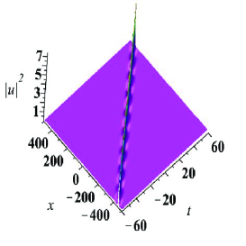
(a) $|q|^{2}$

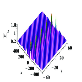
(b) $|q|^{2}$

(c) $|q|^{2}$

Figure 1: (color online): Parameters $\beta=1$, $\gamma=5$: (a) Single breather solution. Parameters: $a_{1}=0$, $\varphi_{1}=\ln(2+\sqrt{5})+\frac{\pi}{2}\mathrm{i}$, (b) Akhmediev breather solution. Parameters: $a_{1}=0$, $\varphi_{1}=\frac{\pi}{3}\mathrm{i}$, (c)Two breather solution. Parameters: $\varphi_{1}=\ln(2+\sqrt{5})+\frac{\pi}{2}\mathrm{i}$, $\varphi_{2}=\frac{\pi}{3}\mathrm{i}$, $a_{1}=a_{2}=0$.

If $(\varphi_{1,R},\varphi_{1,I})\in\Omega_{1}\equiv\{(\varphi_{R},\varphi_{I})|0\leq\varphi_{R}<\mathrm{arcsinh}(\frac{\beta}{\gamma}),\,\,\arccos(-\frac{\gamma}{\beta}\sinh(\varphi_{R}))<\varphi_{I}<\pi\}$, then the single breather $|q[1]|^{2}$ propagates with velocity $\frac{2}{\gamma}v_{1}\leq 0$. If $(\varphi_{1,R},\varphi_{1,I})\in\Omega_{2}\equiv\{(\varphi_{R},\varphi_{I})|\frac{\pi}{2}\leq\varphi_{I}<\pi,\,\,\mathrm{arcsinh}(-\frac{\gamma}{\beta}\cos(\varphi_{I}))<\varphi_{R}\}$, then the single breather $|q[1]|^{2}$ propagates with velocity $\frac{2}{\gamma}v_{1}>0$. An example of this case is illustrated in Fig. 1 (a). If $\gamma\sinh\left(\varphi_{1,R}\right)+\beta\cos\left(\varphi_{1,I}\right)=0$, then we can obtain the so-called Akhmediev breather, which is periodic in time and localized in space. Fig. 1 (b) shows an example of Akhmediev breather.

To analyze the dynamics of the breather solution for the CSP equation (2), we need to solve the relation between $(x,t)$ and $(y,s)$. Although, it is not possible in general, we can obtain the relation at special location $\theta_{1,R}=0$ and $\theta_{1,I}=k\pi+\frac{\pi}{4}$, that is, $s=-t$ and $y=-\frac{2}{\gamma}(x-\frac{\beta^{2}}{8}t).$ It follows that

$$\begin{split}\theta_{1,R}&=-\frac{\gamma}{2}\delta_{1}\left[x-\left(v_{1}+\frac{\beta^{2}}{8}\right)t\right]-\varphi_{1,R}+a_{1,R},\\ \theta_{1,I}&=-\frac{\gamma}{2}\epsilon_{1}\left[x-\left(w_{1}+\frac{\beta^{2}}{8}\right)t\right]-\varphi_{1,I}+a_{1,I}\,.\end{split}$$

The breather solution $|q[1]|^{2}$ propagates with the velocity $v_{1}+\frac{\beta^{2}}{8}$ (Fig.1 a). If $\delta_{1}=0$, we can obtain the Akhmediev breather (Fig.1b). The periodic in $x$ direction is $\frac{2\pi}{\gamma|\epsilon_{1}|},$ the periodic in $t$ direction is $\frac{2\pi}{\gamma|\epsilon_{1}|\left(w_{1}+\frac{\beta^{2}}{8}\right)}.$ The peak value of $|q[1]|^{2}$ is located at

$$\begin{split}x=&\frac{1}{v_{1}-w_{1}}\left[-\frac{2\left(v_{1}+\frac{\beta^{2}}{8}\right)}{\gamma\epsilon_{1}}\left(\frac{\pi}{4}+k\pi+(\varphi_{1,I}-a_{1,I})\right)-\frac{2}{\gamma}\frac{a_{1,R}-\varphi_{1,R}}{\delta_{1}}\left(w_{1}+\frac{\beta^{2}}{8}\right)\right],\\ t=&\frac{1}{v_{1}-w_{1}}\left[-\frac{2}{\gamma\epsilon_{1}}\left(\frac{\pi}{4}+k\pi+(\varphi_{1,I}-a_{1,I})\right)-\frac{2}{\gamma}\frac{a_{1,R}-\varphi_{1,R}}{\delta_{1}}\right].\end{split}$$

Similar to three cases of the single soliton solution, we can classify the single breather solution by defining

$$\begin{split}M_{1}=&\frac{1}{2}{\beta}^{3}\sinh(2\varphi_{1,R})\sin(2\varphi_{1,I})-\gamma\left[(\cosh(\varphi_{1,R})-\cos(\varphi_{1,I}))^{2}+2\cosh(\varphi_{1,R})\sin(\varphi_{1,I})\right]{\beta}^{2}\\ &-2\beta{\gamma}^{2}\sinh(\varphi_{1,R})\cos(\varphi_{1,I})+{\gamma}^{3}.\end{split}$$ (39)

It can be shown that if $M_{1}>0$, the breather solution is a smooth one; if $M_{1}=0$, the breather becomes a cusponed one, in which $|q_{x}|\rightarrow\infty$ at the peak point; if $M_{1}<0$, then we have a looped breather, which is a multi-valued solution.

Generally, through the formula (28) we have the following $N$-breather solution:

$$\begin{split}q[N]&=\frac{\beta}{2}\left[\frac{\det(G)}{\det(M)}\right]\mathrm{e}^{\mathrm{i}\theta},\\ x&=-\frac{\gamma}{2}y-\frac{\beta^{2}}{8}s-2\ln_{s}(\det(M)),\,\,t=-s,\end{split}$$ (40)

where

$$\begin{split}M&=\left(\left[\frac{\mathrm{e}^{2(\theta_{i}^{\ast}+\theta_{j})}}{\xi_{i}^{\ast}-\xi_{j}}+\frac{\mathrm{e}^{2\theta_{i}^{\ast}}}{\xi_{i}^{\ast}-\chi_{j}}+\frac{\mathrm{e}^{2\theta_{j}}}{\chi_{i}^{\ast}-\xi_{j}}+\frac{1}{\chi_{i}^{\ast}-\chi_{j}}\right]\mathrm{e}^{-(\theta_{i}^{\ast}+\theta_{j})}\right)_{1\leq i,j\leq N},\,\,\\ G&=\left(\left[\frac{\xi_{i}^{\ast}+\gamma}{\xi_{j}+\gamma}\frac{\mathrm{e}^{2(\theta_{i}^{\ast}+\theta_{j})}}{\xi_{i}^{\ast}-\xi_{j}}+\frac{\xi_{i}^{\ast}+\gamma}{\chi_{j}+\gamma}\frac{\mathrm{e}^{2\theta_{i}^{\ast}}}{\xi_{i}^{\ast}-\chi_{j}}+\frac{\chi_{i}^{\ast}+\gamma}{\xi_{j}+\gamma}\frac{\mathrm{e}^{2\theta_{j}}}{\chi_{i}^{\ast}-\xi_{j}}+\frac{\chi_{i}^{\ast}+\gamma}{\chi_{j}+\gamma}\frac{1}{\chi_{i}^{\ast}-\chi_{j}}\right]\mathrm{e}^{-(\theta_{i}^{\ast}+\theta_{j})}\right)_{1\leq i,j\leq N}.\end{split}$$

The dynamics for $N$-breather solution is a very interesting topic. It is naturally to conjecture that the $N$-breather solution possesses the same law as the $N$-bright soliton solution. To understand the $N$-breather solution for the CSP equation (40), we first give the following asymptotical analysis for the CCD equation (3):

Proposition 5

Suppose $v_{1}<v_{2}<\cdots<v_{l}\leq 0<v_{N}<v_{N-1}<\cdots<v_{l+1}$. When $s\rightarrow-\infty$, we have

$$\begin{split}q[N]=&\frac{\beta}{2}\left[q_{1}^{-}+\left(q_{2}^{-}-\mathrm{e}^{-2\mathrm{i}\varphi_{1,I}}\Theta_{1}^{-}\right)+\cdots+\left(q_{k}^{-}-\mathrm{e}^{-2\mathrm{i}\varphi_{k-1,I}}\Theta_{k-1}^{-}\right)+\left(q_{N}^{-}-\mathrm{e}^{-2\mathrm{i}\varphi_{k,I}}\Theta_{k}^{-}\right)\right.\\ &\left.+\left(q_{N-1}^{-}-\mathrm{e}^{2\mathrm{i}\varphi_{N,I}}\Theta_{N}^{-}\right)+\cdots+\left(q_{k+1}^{-}-\mathrm{e}^{2\mathrm{i}\varphi_{k+1,I}}\Theta_{k+2}^{-}\right)\right]\mathrm{e}^{\mathrm{i}\theta}+O(\mathrm{e}^{-c|s|}),\end{split}$$ (41)

where $c=\frac{2}{\gamma}\mathrm{min}(\delta_{i})\mathrm{min}_{i\neq j}(|v_{i}-v_{j}|)$. When $s\rightarrow+\infty$, we have

$$\begin{split}q[N]=&\frac{\beta}{2}\left[q_{1}^{+}+\left(q_{2}^{+}-\mathrm{e}^{2\mathrm{i}\varphi_{1,I}}\Theta_{1}^{+}\right)+\cdots+\left(q_{k}^{+}-\mathrm{e}^{2\mathrm{i}\varphi_{k-1,I}}\Theta_{k-1}^{+}\right)+\left(q_{N}^{+}-\mathrm{e}^{2\mathrm{i}\varphi_{k,I}}\Theta_{k}^{+}\right)\right.\\ &\left.+\left(q_{N-1}^{+}-\mathrm{e}^{-2\mathrm{i}\varphi_{N,I}}\Theta_{N}^{+}\right)+\cdots+\left(q_{k+1}^{+}-\mathrm{e}^{-2\mathrm{i}\varphi_{k+1,I}}\Theta_{k+2}^{+}\right)\right]\mathrm{e}^{\mathrm{i}\theta}+O(\mathrm{e}^{-c|s|}),\end{split}$$ (42)

where

$$q_{k}^{\pm}=\Theta_{k}^{\pm}\left[\frac{\cosh(2\theta_{k,R}^{\pm}-2\mathrm{i}\varphi_{k,I})\cosh(\varphi_{k,R})+\sin(2\theta_{k,I}^{\pm}+2\mathrm{i}\varphi_{k,I})\sin(\varphi_{k,I})}{\cosh(2\theta_{k,R}^{\pm})\cosh(\varphi_{k,R})-\sin(2\theta_{k,I}^{\pm})\sin(\varphi_{k,I})}\right],$$

and

$$\begin{split}\theta_{k,R}^{+}=&\theta_{k,R}+\Delta_{k,R}^{+},\,\,\Delta_{k,R}^{+}=\frac{1}{2}\left[\bigstar\ln\left|\frac{\chi_{n}-\xi_{k}}{\chi_{n}^{\ast}-\xi_{k}}\right|\left|\frac{\chi_{n}^{\ast}-\chi_{k}}{\chi_{n}-\chi_{k}}\right|+\blacklozenge\ln\left|\frac{\xi_{n}-\xi_{k}}{\xi_{n}^{\ast}-\xi_{k}}\right|\left|\frac{\xi_{n}^{\ast}-\chi_{k}}{\xi_{n}-\chi_{k}}\right|\right],\\ \theta_{k,I}^{+}=&\theta_{k,I}+\Delta_{k,I}^{+},\,\,\Delta_{k,I}^{+}=\frac{1}{2}\left[\bigstar\arg\left(\frac{\chi_{n}-\xi_{k}}{\chi_{n}^{\ast}-\xi_{k}}\frac{\chi_{k}^{\ast}-\chi_{n}^{\ast}}{\chi_{k}^{\ast}-\chi_{n}}\right)+\blacklozenge\arg\left(\frac{\xi_{n}-\xi_{k}}{\xi_{n}^{\ast}-\xi_{k}}\frac{\chi_{k}^{\ast}-\xi_{n}^{\ast}}{\chi_{k}^{\ast}-\xi_{n}}\right)\right],\\ \theta_{k,R}^{-}=&\theta_{k,R}+\Delta_{k,R}^{-},\,\,\Delta_{k,R}^{-}=\frac{1}{2}\left[\bigstar\ln\left|\frac{\xi_{n}-\xi_{k}}{\xi_{n}^{\ast}-\xi_{k}}\right|\left|\frac{\xi_{n}^{\ast}-\chi_{k}}{\xi_{n}-\chi_{k}}\right|+\blacklozenge\ln\left|\frac{\chi_{n}-\xi_{k}}{\chi_{n}^{\ast}-\xi_{k}}\right|\left|\frac{\chi_{n}^{\ast}-\chi_{k}}{\chi_{n}-\chi_{k}}\right|\right],\\ \theta_{k,I}^{-}=&\theta_{k,I}+\Delta_{k,I}^{-},\,\,\Delta_{k,I}^{-}=\frac{1}{2}\left[\bigstar\arg\left(\frac{\xi_{n}-\xi_{k}}{\xi_{n}^{\ast}-\xi_{k}}\frac{\chi_{k}^{\ast}-\xi_{n}^{\ast}}{\chi_{k}^{\ast}-\xi_{n}}\right)+\blacklozenge\arg\left(\frac{\chi_{n}-\xi_{k}}{\chi_{n}^{\ast}-\xi_{k}}\frac{\chi_{k}^{\ast}-\chi_{n}^{\ast}}{\chi_{k}^{\ast}-\chi_{n}}\right)\right],\\ \Theta_{k}^{+}=&\exp\left(\bigstar 2\mathrm{i}\varphi_{n,I}-\blacklozenge 2\mathrm{i}\varphi_{n,I}\right),\,\,\Theta_{k}^{-}=\exp\left(-\bigstar 2\mathrm{i}\varphi_{n,I}+\blacklozenge 2\mathrm{i}\varphi_{n,I}\right),\end{split}$$ (43)

if $1\leq k\leq l$, then $\bigstar=\left(\sum_{n=1}^{k-1}+\sum_{n=l+1}^{N}\right),\,\,\blacklozenge=\sum_{n=k+1}^{l};$ if $l<k\leq N$, then $\bigstar=\sum_{n=1}^{k-1},\,\,\blacklozenge=\sum_{n=k+1}^{N};$ and

$$\theta_{i,R}=\delta_{i}\left(y-\frac{2}{\gamma}v_{i}s\right)-\varphi_{i,R}+a_{i,R},\,\,\theta_{i,I}=\epsilon_{i}\left(y-\frac{2}{\gamma}w_{i}s\right)-\varphi_{i,I}+a_{i,I},$$

and

$$\begin{split}v_{i}&=\frac{\alpha_{i}\gamma\sinh\left(\varphi_{i,R}\right)}{4\left(\gamma\sinh\left(\varphi_{i,R}\right)+\beta\cos\left(\varphi_{i,I}\right)\right)},\,\,\delta_{i}=\frac{2\beta}{\alpha_{i}}\sin\left(\varphi_{i,I}\right)\left(\gamma\sinh\left(\varphi_{i,R}\right)+\beta\cos\left(\varphi_{i,I}\right)\right),\\ w_{i}&=\frac{-\alpha_{i}\gamma\cos(\varphi_{i,I})}{4\left(\beta\sinh\left(\varphi_{i,R}\right)-\gamma\cos(\varphi_{i,I})\right)},\,\,\epsilon_{i}=\frac{2\beta}{{\alpha_{i}}}\cosh(\varphi_{i,R})\left(\beta\sinh\left(\varphi_{i,R}\right)-\gamma\cos(\varphi_{i,I})\right),\\ \alpha_{i}&=\left(\beta\sinh\left(\varphi_{i,R}\right)\cos\left(\varphi_{i,I}\right)-\gamma\right)^{2}+{\beta}^{2}\cosh^{2}\left(\varphi_{i,R}\right)\sin^{2}\left(\varphi_{i,I}\right).\end{split}$$

Based on the above proposition, we can obtain the dynamics of $N$-breather solution for the CSP equation (2). In general, the dynamics of $N$-breather solution for the CSP equation (2) cannot be solved analytically. However, in some special location, we can analyze them by the coordinate transformation. When $s\rightarrow\pm\infty$, $\theta_{k,R}^{\pm}=0$ and $\theta_{k,I}^{\pm}=\frac{\pi}{4}+k\pi$, we have

$$\begin{split}x&=-\frac{\gamma}{2}y-\frac{\beta^{2}}{8}s-2\ln_{s}(\det(M))\\ &\rightarrow-\frac{\gamma}{2}y-\frac{\beta^{2}}{8}s-2\ln_{s}\left(\exp\left[\pm 2\left(-\bigstar\theta_{n,R}+\blacklozenge\theta_{n,R}\right)\right]\exp\left[-2\theta_{k,R}\right]\det(M_{k})\right),\\ &=-\frac{\gamma}{2}y-\frac{\beta^{2}}{8}s\pm\tau_{k},\end{split}$$

where

$$\tau_{k}=\beta\left(\bigstar\sin(\varphi_{n,I})\sinh(\varphi_{n,R})-\blacklozenge\sin(\varphi_{n,I})\sinh(\varphi_{n,R})\right).$$

Proposition 6

When $t\rightarrow\mp\infty$, along the trajectory $\theta_{k,R}^{\pm}=0$ and $\theta_{k,I}^{\pm}=\frac{\pi}{4}+k\pi$, we have

$$q[N]=\frac{\beta}{2}q_{k}^{\pm}\mathrm{e}^{\mathrm{i}\theta}+O(\mathrm{e}^{-c|t|}),$$

where

$$\begin{split}\theta_{k,R}^{\pm}=&-\frac{\gamma}{2}\delta_{k}\left[x-\left(v_{k}+\frac{\beta^{2}}{8}\right)t\mp\tau_{k}\right]-\varphi_{k,R}+a_{k,R}+\Delta_{k,R}^{\pm},\\ \theta_{k,I}^{\pm}=&-\frac{\gamma}{2}\epsilon_{k}\left[x-\left(w_{k}+\frac{\beta^{2}}{8}\right)t\mp\tau_{k}\right]-\varphi_{k,I}+a_{k,I}+\Delta_{k,I}^{\pm}.\end{split}$$

IV General rogue wave solution to the CSP equation

In previous section, we solved the linear system (5) with plane wave seed solution under the restriction $\lambda_{i}\neq-\gamma+\mathrm{i}\beta$. It is natural to ask what happens if $\lambda_{i}=-\gamma+\mathrm{i}\beta$. Actually, we can obtain the rogue wave solution and high order rogue wave solutions under this special condition. The general procedure to yield these solutions was proposed in Guo1 ; Guo2 .

Starting from the linear system (5) with $(q,\rho,\lambda)=(q[0],\rho[0],-\gamma+\mathrm{i}\beta)$, where $q[0]$ and $\rho[0]$ are given in equation (36), then one can firstly obtain the quasi-rational solution, from which the first order rogue wave solution can be obtained through formula (28). However, the higher order RW solution cannot be constructed in the same way. To find the general higher order rogue wave solution, we need to solve the linear system (5) with $(q,\rho,\lambda)=(q[0],\rho[0],-\gamma+\mathrm{i}\beta-\frac{\mathrm{i}\epsilon^{2}}{2\beta})$, where $\epsilon$ is a small parameter.

To this end, we give the following Lemma.

Lemma 1

Denote

$$\lambda_{1}=-\gamma+\mathrm{i}\beta-\frac{\mathrm{i}\epsilon^{2}}{2\beta},\,\,\mu_{1}=\epsilon\sqrt{1-\left(\frac{\epsilon}{2\beta}\right)^{2}},\,\,\xi_{1}=\lambda_{1}+\mu_{1},$$ (44)

then the following parameters can be expanded in terms of a small parameter $\epsilon$

$$\begin{split}\mu_{1}&=\sum_{n=0}^{\infty}\mu_{1}^{[n]}\epsilon^{2n+1},\\ \frac{1}{\xi_{1}^{\ast}-\xi_{1}}&=\sum_{i=0,j=0}^{\infty,\infty}F^{[i,j]}\epsilon^{\ast i}\epsilon^{j},\\ \frac{1}{\xi_{1}+\gamma}&\equiv\frac{1}{\mathrm{i}\beta(\sqrt{1-\epsilon^{2}}-\mathrm{i}\epsilon)^{2}}=\sum_{i=0}^{\infty}J^{[i]}\epsilon^{i},\end{split}$$

where

$$\begin{split}\mu_{1}^{[n]}&=\begin{pmatrix}\frac{1}{2}\\[5.0pt] n\\ \end{pmatrix}\left(\frac{-1}{4\beta^{2}}\right)^{n},\,\,\begin{pmatrix}\frac{1}{2}\\[5.0pt] n\\ \end{pmatrix}=\frac{\frac{1}{2}(\frac{1}{2}-1)\cdots(\frac{1}{2}-n+1)}{n!},\\ F^{[i,j]}&=\frac{\mathrm{i}}{i!j!\beta}\frac{\partial^{i+j}}{\partial\epsilon^{\ast i}\partial\epsilon^{j}}\left(\left[\exp\left(2\mathrm{i}\arcsin\left(\frac{\epsilon^{\ast}}{2\beta}\right)\right)+\exp\left(-2\mathrm{i}\arcsin\left(\frac{\epsilon}{2\beta}\right)\right)\right]^{-1}\right)_{|_{\epsilon^{\ast}=0,\epsilon=0}},\\ J^{[0]}=&\frac{1}{\mathrm{i}\beta},\,\,J^{[1]}=\frac{1}{\beta^{2}},\,\,J^{[2]}=\frac{\mathrm{i}}{2\beta^{3}},\,\,J^{[2i+1]}=\frac{(-1)^{i}}{\beta^{2}}\begin{pmatrix}\frac{1}{2}\\[8.0pt] i\\ \end{pmatrix}\left(\frac{1}{2\beta}\right)^{2i},\,\,J^{[2i+2]}=0,\,\,i\geq 1.\end{split}$$

With the aid of above lemma, we have the following expansion

$$\begin{split}X_{1}&\equiv\frac{\mathrm{i}}{4}\mu_{1}\left(s+{\frac{2y}{\lambda}}+\sum_{i=1}^{\infty}(a_{i}+\mathrm{i}b_{i})\epsilon^{2i}\right)+\frac{1}{2}\ln\left({\frac{\mu_{1}+\lambda_{1}+\gamma}{\mathrm{i}\beta}}\right),\\ &=\mathrm{i}\epsilon\left(\sum_{i=1}^{\infty}\frac{\mu_{1}^{[i]}}{4}\epsilon^{2i}\right)\left(\sum_{i=0}^{\infty}K^{[i]}\epsilon^{2i}\right)-\mathrm{i}\arcsin\left(\frac{\epsilon}{2\beta}\right)\\ &=\mathrm{i}\epsilon\sum_{k=0}^{\infty}X_{1}^{[2k+1]}\epsilon^{2k},\end{split}$$

where

$$\begin{split}X_{1}^{[2k+1]}&=\left[\sum_{j=0}^{k}\frac{1}{4}K^{[j]}\mu_{1}^{[k-j]}-\frac{(-1)^{k}}{2k+1}\begin{pmatrix}-\frac{1}{2}\\[5.0pt] k\\ \end{pmatrix}\right],\\ K^{[k]}&=\left\{\begin{array}[]{ll}{\displaystyle s-\frac{2(\gamma+\mathrm{i}\beta)y}{\beta^{2}+\gamma^{2}}},&k=0,\\[8.0pt] {\displaystyle\left(\frac{-2(\gamma+\mathrm{i}\beta)y}{\gamma^{2}+\beta^{2}}\right)\left(\frac{(\gamma+\mathrm{i}\beta)}{2\beta(\gamma^{2}+\beta^{2})\mathrm{i}}\right)^{k}}+a_{k}+\mathrm{i}b_{k},&k\geq 1.\end{array}\right.\end{split}$$

Furthermore we have

$$\mathrm{e}^{X_{1}}=\sum_{i=0}^{\infty}S_{i}(\mathbf{X}_{1})\epsilon^{i},\,\,\mathbf{X}_{1}=\left(X_{1}^{[1]},X_{1}^{[2]},\cdots\right),\,\,X_{1}^{[2k]}=0,\,\,k\geq 1,\\$$

where $S_{i}(\mathbf{X}_{1})$ are elementary Schur polynomials

$$\begin{split}S_{0}(\mathbf{X}_{1})=&1,\,\,S_{1}(\mathbf{X}_{1})=X_{1}^{[1]},\,\,S_{2}(\mathbf{X}_{1})=X_{1}^{[2]}+\frac{(X_{1}^{[1]})^{2}}{2},\,\,S_{3}(\mathbf{X}_{1})=X_{1}^{[3]}+X_{1}^{[1]}X_{1}^{[2]}+\frac{(X_{1}^{[1]})^{3}}{6},\cdots\\ S_{i}(\mathbf{X}_{1})=&\sum_{l_{1}+2l_{2}+\cdots+kl_{k}=i}\frac{(X_{1}^{[1]})^{l_{1}}(X_{1}^{[2]})^{l_{2}}\cdots(X_{1}^{[k]})^{l_{k}}}{l_{1}!l_{2}!\cdots l_{k}!}.\end{split}$$

Since $KE_{1}(\epsilon)$ satisfies the Lax equation (5), then $KE_{1}(-\epsilon)$ also satisfies the Lax equation (5). To obtain the general higher order rogue wave solution, we choose the general special solution

$$|y_{1}\rangle=\frac{K}{2\epsilon}\left[E_{1}(\epsilon)-E_{1}(-\epsilon)\right]\equiv K\begin{bmatrix}\varphi_{1}\\ \beta\psi_{1}\\ \end{bmatrix},\quad E_{1}=\begin{bmatrix}\mathrm{e}^{X_{1}}\\ {\displaystyle\frac{\beta\mathrm{e}^{X_{1}}}{\xi_{1}+\gamma}}\\ \end{bmatrix}\,.$$

Finally, we have

$$\frac{\langle y_{1}|y_{1}\rangle}{2(\lambda_{1}^{*}-\lambda_{1})}=\frac{1}{4}\left[\frac{\mathrm{e}^{X_{1}^{*}+X_{1}}}{\xi_{1}^{*}-\xi_{1}}-\frac{\mathrm{e}^{X_{1}^{*}-X_{1}}}{\xi_{1}^{*}-\chi_{1}}-\frac{\mathrm{e}^{-X_{1}^{*}+X_{1}}}{\chi_{1}^{*}-\xi_{1}}+\frac{\mathrm{e}^{-X_{1}^{*}-X_{1}}}{\chi_{1}^{*}-\chi_{1}}\right]=\sum_{m=1,n=1}^{\infty,\infty}M^{[m,n]}{\epsilon}^{*2(m-1)}\epsilon^{2(n-1)},$$ (45)

where $\chi_{1}=\xi_{1}(-\epsilon),$

$$M^{[m,n]}=\sum_{i=0}^{2m-1}\sum_{j=0}^{2n-1}F^{[i,j]}S_{2n-i-1}(X_{1})S_{2m-j-1}(X_{1}^{*}).$$

On the other hand, by using lemma 1, we have the following expansion

$$\varphi_{1}=\frac{1}{2}\left(\mathrm{e}^{X_{1}}-\mathrm{e}^{-X_{1}}\right)=\sum_{n=1}^{\infty}\varphi_{1}^{[n]}\epsilon^{2(n-1)},\,\,\psi_{1}=\frac{1}{2}\left(\frac{\mathrm{e}^{X_{1}}}{\xi_{1}+\gamma}-\frac{\mathrm{e}^{-X_{1}}}{\chi_{1}+\gamma}\right)=\sum_{n=1}^{\infty}\psi_{1}^{[n]}\epsilon^{2(n-1)}\,,$$ (46)

where

$$\varphi_{1}^{[n]}=S_{2n-1}(\mathbf{X}_{1}),\,\,\psi_{1}^{[n]}=\sum_{k=0}^{2n-1}S_{k}(\mathbf{X}_{1})J_{1}^{[2n-1-k]}.$$

Based on the expansion equations (45)-(46), and formulas (27)-(28)-(24), we can obtain the general rogue wave solutions:

Proposition 7

The general higher order rogue wave solution for the CSP equation (2) can be represented as

$$\begin{split}q[N]&=\frac{\beta}{2}\left[\frac{\det(G)}{\det(M)}\right]\mathrm{e}^{\mathrm{i}\theta},\\ x&=-\frac{\gamma}{2}y-\frac{{\beta}^{2}}{8}s-2\ln_{s}(\det(M)),\,\,t=-s,\end{split}$$ (47)

where

$$M=\left(M^{[m,n]}\right)_{1\leq m,n\leq N},\,\,G=\left(M^{[m,n]}+\varphi_{1}^{[m]\ast}\psi_{1}^{[n]}\right)_{1\leq m,n\leq N}.$$

Specifically, the first order rogue wave solution can be written explicitly through formula (47)

$$\begin{split}q[1]=&\frac{\beta}{2}\left[1+\frac{16(\mathrm{i}{\beta}^{2}y-{\beta}^{2}-{\gamma}^{2})}{\beta^{2}\left(2y-\gamma s\right)^{2}+{\beta}^{4}{s}^{2}+4\gamma^{2}+4{\beta}^{2}}\right]\mathrm{e}^{\mathrm{i}\theta},\\ x=&-\frac{\gamma}{2}y-\frac{{\beta}^{2}}{8}s-\frac{4{\beta}^{2}\left({\gamma}^{2}s+{\beta}^{2}s-2\gamma y\right)}{\beta^{2}\left(2y-\gamma s\right)^{2}+{\beta}^{4}{s}^{2}+4\gamma^{2}+4{\beta}^{2}},\,\,t=-s.\end{split}$$ (48)

It can be shown that if $\beta^{2}<\frac{\gamma^{2}}{3}$, then one has the regular rogue wave solution (Fig. 2); if $\beta^{2}=\frac{\gamma^{2}}{3}$, then one obtains the cusponed rogue wave solution, in which $|q_{x}|\rightarrow\infty$ at the peak point (Fig. 3); if $\beta^{2}>\frac{\gamma^{2}}{3}$, then we has the looped rogue wave solution (Fig. 4). Although both the NLS and the CSP equations possess the modulational instability (see the Appendix), the rogue wave solution of the CSP equation (2) could yield the singularity which is different from the NLS equation. This solution may be related to the wave breaking in the CSP equation.

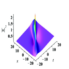
(a) $|q|^{2}$

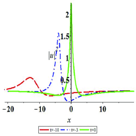
(b) $|q|^{2}$

Figure 2: (color online): Parameters: $\beta=1$, $\gamma=2$, (a) The spatio-temporal pattern for the regular first order RW, (b) The figure of $|q[1]|^{2}$ for different time, it is seen that the amplitude is variation.

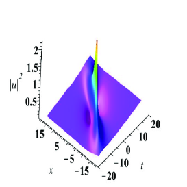
(a) $|q|^{2}$

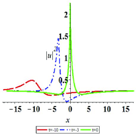
(b) $|q|^{2}$

Figure 3: (color online): Parameters: $\beta=1$, $\gamma=\sqrt{3}$, (a) The spatio-temporal pattern for the first order wave-breaking RW, (b) The figure of $|q[1]|^{2}$ for different time, it is seen that the derivative for the amplitude $|q|^{2}$ at $(x,t)=(0,0)$ is very large.

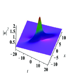
(a) $|q|^{2}$

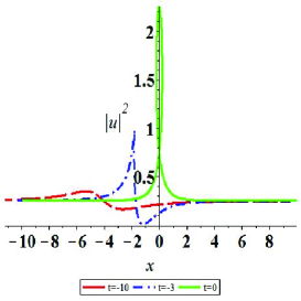
(b) $|q|^{2}$

Figure 4: (color online): Parameters: $\beta=1$, $\gamma=1$, (a) The spatio-temporal pattern for the first order loop RW, (b) The figure of $|q[1]|^{2}$ for different time, it is seen that the amplitude $|q|^{2}$ at $t=-10$ is regular, but when $t=0$, it appears a loop.

By the formula (28), the second order rogue wave solution can be calculated as

$$\begin{split}q[2]=&\frac{\beta}{2}\left[1+\frac{G_{2}}{M_{2}}\right]\mathrm{e}^{\mathrm{i}\theta},\\ x=&-\frac{\gamma}{2}y-\frac{{\beta}^{2}}{8}s-2\ln_{s}(M_{2}),\,\,t=-s,\end{split}$$ (49)

where

$$\begin{split}M_{2}=&\beta^{6}A\hat{y}^{6}+\left[3{\beta}^{6}A\hat{s}^{2}+12{\beta}^{6}+108{\beta}^{4}{\gamma}^{2}\right]\hat{y}^{4}+\left[-288\gamma{\beta}^{5}\hat{s}-96b_{{1}}A{\beta}^{6}\right]\hat{y}^{3}\\ &+\left[3{\beta}^{6}A\hat{s}^{4}+\left(-72{\beta}^{4}{\gamma}^{2}+216{\beta}^{6}\right)\hat{s}^{2}-288a_{{1}}{\beta}^{6}A\hat{s}+432{\beta}^{4}+1584{\gamma}^{2}{\beta}^{2}\right]\hat{y}^{2}\\ &+\left[96\gamma{\beta}^{5}\hat{s}^{3}+288Ab_{{1}}{\beta}^{6}\hat{s}^{2}-1152\gamma{\beta}^{3}\hat{s}+4608a_{{1}}{\beta}^{5}\gamma+1152b_{{1}}{\beta}^{6}-3456b_{{1}}{\beta}^{4}{\gamma}^{2}\right]\hat{y}\\ &+A\left[{\beta}^{6}\hat{s}^{6}+12{\beta}^{4}\hat{s}^{4}+96a_{{1}}{\beta}^{6}\hat{s}^{3}+432{\beta}^{2}\hat{s}^{2}-1152a_{{1}}{\beta}^{4}\hat{s}+576+2304\left({a_{1}}^{2}+{b_{1}}^{2}\right){\beta}^{6}\right],\\ G_{2}=&a_{{1}}{\beta}^{4}A\left(2304\mathrm{i}\beta\hat{y}+4068\right)\hat{s}+A\left[1152\mathrm{i}{\beta}^{5}\left({\hat{y}}^{2}-\hat{s}^{2}\right)+4068{\beta}^{4}\hat{y}-4608\mathrm{i}{\beta}^{3}\right]b_{{1}}\\ &-24\mathrm{i}A{\beta}^{5}{\hat{y}}^{5}-240{\beta}^{4}A{\hat{y}}^{4}+\left[-48\mathrm{i}A{\beta}^{5}\hat{s}^{2}-192\mathrm{i}{\gamma}^{2}{\beta}^{3}+960\mathrm{i}{\beta}^{5}\right]\hat{y}^{3}\\ &+\left[-288{\beta}^{4}A\hat{s}^{2}+2304\mathrm{i}\gamma{\beta}^{4}\hat{s}-3456{\gamma}^{2}{\beta}^{2}+1152{\beta}^{4}\right]{\hat{y}}^{2}\\ &+\left[-24\mathrm{i}A{\beta}^{5}\hat{s}^{4}+576\mathrm{i}\left({\gamma}^{2}-{\beta}^{2}\right){\beta}^{3}\hat{s}^{2}+4608{\beta}^{3}\gamma\hat{s}+5760\mathrm{i}{\gamma}^{2}\beta+1152\mathrm{i}{\beta}^{3}\right]\hat{y}\\ &-A(48{\beta}^{4}\hat{s}^{4}+1152{\beta}^{2}\hat{s}^{2}-2304)\end{split}$$ (50)

and

$$\hat{s}=s-\frac{2\gamma y}{A},\,\,\hat{y}=\frac{-2\beta y}{A},\,\,A=\beta^{2}+\gamma^{2}.$$

The spatio-temporal pattern of the second order RW solution is similar to the ones of the NLS equation Guo1 or derivative NLS equation Guo2 . An example is shown in (Fig. 5b). For the general case, it is impossible to describe their dynamics analytically. However for the standard case $a_{1}=b_{1}=0$, it is shown that if $\beta^{2}<\left(1-\frac{2\sqrt{5}}{5}\right)\gamma^{2}$, one obtains the regular rogue wave (Fig. 5a); if $\beta^{2}=\left(1-\frac{2\sqrt{5}}{5}\right)\gamma^{2}$, one can obtain the cuspon-type rogue wave; if $\beta^{2}>\left(1-\frac{2\sqrt{5}}{5}\right)\gamma^{2}$, one arrives at the loop-type rogue wave (Fig. 6).

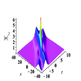
(a) $|q|^{2}$

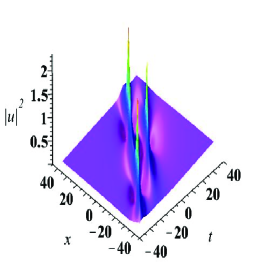
(b) $|q|^{2}$

Figure 5: (color online): (a)The second order regular RW; Parameters: $\beta=1$, $\gamma=4$, $a_{1}=b_{1}=0$, (b) The second order regular RW; Parameters: $\beta=1$, $\gamma=2$, $a_{1}=20,b_{1}=0$,

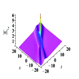
(a) $|q|^{2}$

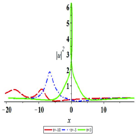
(b) $|q|^{2}$

Figure 6: (color online): Parameters: $\beta=1$, $\gamma=2$, $a_{1}=b_{1}=0$ (a): The second order loop RW; (b) The different time of $|q[2]|^{2}$.

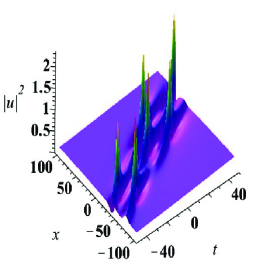
(a) $|q|^{2}$

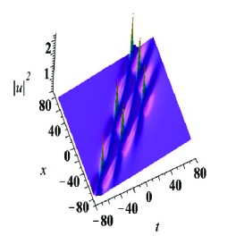
(b) $|q|^{2}$

Figure 7: (color online): (a)The third order RW with pentagon arrangement. Parameters: $\beta=1$, $\gamma=2$, $a_{2}=500$, $a_{1}=0$, $b_{1}=b_{2}=0$, (b) The third order RW with triangle arrangement. $\beta=1$, $\gamma=2$, $a_{2}=0$, $a_{1}=100$, $b_{1}=b_{2}=0$,

The expression for the higher order rogue wave solution $N\geq 3$ becomes very complicated. Here, we only illustrate a third-order rogue wave solution (Fig. 7) without providing an analytical expression.

V Conclusions and discussions

In the present paper, we study the complex short pulse (CSP) equation by Darboux transformation method. We firstly develop a generalized Darboux transformation (DT) and associated Bäcklund transformation for the complex coupled dispersionless (CCD) equation, which leads to a general soliton formulas for the CCD equation. Then by integrating the reciprocal transformation exactly, the $N$-bright soliton solution in a compact determinant form is constructed. Furthermore, the $N$-breather solution and higher order rogue wave solution to the CSP equation are constructed by a delicate limiting process.

The $N$-bright soliton solution should be equivalent to the ones found by one of the authors Feng2 ; shen , the $N$-breather solution and higher order rogue wave solution are found to the CSP equation for the first time and deserve further study. Especially, this is the first example for the existence of rogue wave solution in a nonlinear wave equation possessing reciprocal (hodograph) transformation. Due to this reciprocal transformation, all the localized solutions including the bright, breather and rogue wave ones can be either smooth, cupson or loop ones. Based on the compact determinant form of the solutions, we perform an asymptotic analysis for the $N$-bright soliton and $N$-breather solutions. It should be pointed out that the method for the asymptotical analysis can be extended to other integrable equations as well. In compared to the NLS equation, the rogue wave solution for the CSP equation (2) could develop into wave-breaking. This illustrates that the modulational instability for the CSP equation (2) is stronger than the NLS equation.

Finally, the CSP equation could be of defocusing type, which admits the dark soliton solution, same as the NLS equation. It turns out that this is indeed the case. The complex short pulse equation of both focusing and defocusing types can be derived from the context of nonlinear optics. The results are summarized in a separate work LingFengdCSP .

Appendix A: Proof of Proposition 3

Proof: Fixed $y-v_{k}s=\mathrm{const}$, and $s\rightarrow-\infty$, it follows that $\theta_{1},\theta_{2},\cdots,\theta_{k-1}\rightarrow-\infty$; $\theta_{k+1},\theta_{k+2},\cdots,\theta_{N}\rightarrow+\infty.$ On the other hand, $q[N]$ can be rewritten as

$$q[N]=-\frac{\det(\widehat{G})}{\det(\widehat{M})},$$ (51)

where

$$\begin{split}\widehat{M}&=\left(\frac{\mathrm{e}^{2(\theta_{i}^{\ast}+\theta_{j})}+1}{\lambda_{i}^{\ast}-\lambda_{j}}\right)_{1\leq i,j\leq N},\,\,\widehat{G}=\begin{bmatrix}\widehat{M}&\widehat{Y_{1}}^{{\dagger}}\\ \widehat{Y_{2}}&0\\ \end{bmatrix},\\ \widehat{Y_{1}}&=\begin{bmatrix}\mathrm{e}^{2\theta_{1}}&\mathrm{e}^{2\theta_{2}}&\cdots&\mathrm{e}^{2\theta_{N}}\\ \end{bmatrix},\,\,\widehat{Y_{2}}=\begin{bmatrix}1&1&\cdots&1\\ \end{bmatrix}.\end{split}$$

It follows that

$$\begin{split}\det(\widehat{M})=&\mathrm{e}^{2(\theta_{k+1}+\theta_{k+2}+\cdots+\theta_{N})}\left[\det(M_{k})+O(\mathrm{e}^{-c|s|})\right],\\ \det(\widehat{G})=&\mathrm{e}^{2(\theta_{k+1}+\theta_{k+2}+\cdots+\theta_{N})}\left[\det(G_{k})+O(\mathrm{e}^{-c|s|})\right],\end{split}$$

where

$$\begin{split}M_{k}&=\begin{bmatrix}\frac{1}{\lambda_{1}^{\ast}-\lambda_{1}}&\cdots&\frac{1}{\lambda_{1}^{\ast}-\lambda_{k-1}}&\frac{1}{\lambda_{1}^{\ast}-\lambda_{k}}&0&\cdots&0\\ \vdots&\ddots&\vdots&\vdots&\vdots&\ddots&\vdots\\ \frac{1}{\lambda_{k-1}^{\ast}-\lambda_{1}}&\cdots&\frac{1}{\lambda_{k-1}^{\ast}-\lambda_{k-1}}&\frac{1}{\lambda_{k-1}^{\ast}-\lambda_{k}}&0&\cdots&0\\ \frac{1}{\lambda_{k}^{\ast}-\lambda_{1}}&\cdots&\frac{1}{\lambda_{k}^{\ast}-\lambda_{k-1}}&\frac{\mathrm{e}^{2(\theta_{k}^{\ast}+\theta_{k})}+1}{\lambda_{k}^{\ast}-\lambda_{k}}&\frac{\mathrm{e}^{2\theta_{k}^{\ast}}}{\lambda_{k}^{\ast}-\lambda_{k+1}}&\cdots&\frac{\mathrm{e}^{2\theta_{k}^{\ast}}}{\lambda_{k}^{\ast}-\lambda_{N}}\\ 0&\cdots&0&\frac{\mathrm{e}^{2\theta_{k}}}{\lambda_{k+1}^{\ast}-\lambda_{k}}&\frac{1}{\lambda_{k+1}^{\ast}-\lambda_{k+1}}&\cdots&\frac{1}{\lambda_{k+1}^{\ast}-\lambda_{N}}\\ \vdots&\ddots&\vdots&\vdots&\vdots&\ddots&\vdots\\ 0&\cdots&0&\frac{\mathrm{e}^{2\theta_{k}}}{\lambda_{N}^{\ast}-\lambda_{k}}&\frac{1}{\lambda_{N}^{\ast}-\lambda_{k+1}}&\cdots&\frac{1}{\lambda_{N}^{\ast}-\lambda_{N}}\\ &&&&&&\end{bmatrix},\\ G_{k}&=\begin{bmatrix}\frac{1}{\lambda_{1}^{\ast}-\lambda_{1}}&\cdots&\frac{1}{\lambda_{1}^{\ast}-\lambda_{k-1}}&\frac{1}{\lambda_{1}^{\ast}-\lambda_{k}}&0&\cdots&0&0\\ \vdots&\ddots&\vdots&\vdots&\vdots&\ddots&\vdots&\vdots\\ \frac{1}{\lambda_{k-1}^{\ast}-\lambda_{1}}&\cdots&\frac{1}{\lambda_{k-1}^{\ast}-\lambda_{k-1}}&\frac{1}{\lambda_{k-1}^{\ast}-\lambda_{k}}&0&\cdots&0&0\\ \frac{1}{\lambda_{k}^{\ast}-\lambda_{1}}&\cdots&\frac{1}{\lambda_{k}^{\ast}-\lambda_{k-1}}&\frac{\mathrm{e}^{2(\theta_{k}^{\ast}+\theta_{k})}+1}{\lambda_{k}^{\ast}-\lambda_{k}}&\frac{\mathrm{e}^{2\theta_{k}^{\ast}}}{\lambda_{k}^{\ast}-\lambda_{k+1}}&\cdots&\frac{\mathrm{e}^{2\theta_{k}^{\ast}}}{\lambda_{k}^{\ast}-\lambda_{N}}&\mathrm{e}^{2\theta_{k}^{\ast}}\\ 0&\cdots&0&\frac{\mathrm{e}^{2\theta_{k}}}{\lambda_{k+1}^{\ast}-\lambda_{k}}&\frac{1}{\lambda_{k+1}^{\ast}-\lambda_{k+1}}&\cdots&\frac{1}{\lambda_{k+1}^{\ast}-\lambda_{N}}&1\\ \vdots&\ddots&\vdots&\vdots&\vdots&\ddots&\vdots&\vdots\\ 0&\cdots&0&\frac{\mathrm{e}^{2\theta_{k}}}{\lambda_{N}^{\ast}-\lambda_{k}}&\frac{1}{\lambda_{N}^{\ast}-\lambda_{k+1}}&\cdots&\frac{1}{\lambda_{N}^{\ast}-\lambda_{N}}&1\\ 1&\cdots&1&1&0&\cdots&0&0\\ &&&&&&&\end{bmatrix}.\end{split}$$

By direct calculation, we have

$$\begin{split}\det(G_{k})=&(-1)^{k+N+1}\begin{vmatrix}\frac{1}{\lambda_{1}^{\ast}-\lambda_{1}}&\cdots&\frac{1}{\lambda_{1}^{\ast}-\lambda_{k-1}}&\frac{1}{\lambda_{1}^{\ast}-\lambda_{k}}\\ \vdots&\ddots&\vdots&\vdots\\ \frac{1}{\lambda_{k-1}^{\ast}-\lambda_{1}}&\cdots&\frac{1}{\lambda_{k-1}^{\ast}-\lambda_{k-1}}&\frac{1}{\lambda_{k-1}^{\ast}-\lambda_{k}}\\ 1&\cdots&1&1\\ &&&\end{vmatrix}\begin{vmatrix}\frac{\mathrm{e}^{2\theta_{k}^{\ast}}}{\lambda_{k}^{\ast}-\lambda_{k+1}}&\cdots&\frac{\mathrm{e}^{2\theta_{k}^{\ast}}}{\lambda_{k}^{\ast}-\lambda_{N}}&\mathrm{e}^{2\theta_{k}^{\ast}}\\ \frac{1}{\lambda_{k+1}^{\ast}-\lambda_{k+1}}&\cdots&\frac{1}{\lambda_{k+1}^{\ast}-\lambda_{N}}&1\\ \vdots&\ddots&\vdots&\vdots\\ \ \frac{1}{\lambda_{N}^{\ast}-\lambda_{k+1}}&\cdots&\frac{1}{\lambda_{N}^{\ast}-\lambda_{N}}&1\\ &&&\end{vmatrix}\\ =&-\prod_{l=1}^{k-1}\left(\frac{\lambda_{l}-\lambda_{k}}{\lambda_{l}^{\ast}-\lambda_{k}}\right)\prod_{l=k+1}^{N}\left(\frac{\lambda_{l}^{\ast}-\lambda_{k}^{\ast}}{\lambda_{l}-\lambda_{k}^{\ast}}\right)C(\lambda_{1}^{\ast},\lambda_{2}^{\ast},\cdots,\lambda_{k-1}^{\ast})C(\lambda_{k+1}^{\ast},\lambda_{k+2}^{\ast},\cdots,\lambda_{N}^{\ast})\mathrm{e}^{2\theta_{k}^{\ast}};\end{split}$$

and

$$\begin{split}&\det(M_{k})\\ =&\begin{vmatrix}\frac{1}{\lambda_{1}^{\ast}-\lambda_{1}}&\cdots&\frac{1}{\lambda_{1}^{\ast}-\lambda_{k}}&0&\cdots&0\\ \vdots&\ddots&\vdots&\vdots&\ddots&\vdots\\ \frac{1}{\lambda_{k-1}^{\ast}-\lambda_{1}}&\cdots&\frac{1}{\lambda_{k-1}^{\ast}-\lambda_{k}}&0&\cdots&0\\ \frac{1}{\lambda_{k}^{\ast}-\lambda_{1}}&\cdots&\frac{1}{\lambda_{k}^{\ast}-\lambda_{k}}&\frac{\mathrm{e}^{2\theta_{k}^{\ast}}}{\lambda_{k}^{\ast}-\lambda_{k+1}}&\cdots&\frac{\mathrm{e}^{2\theta_{k}^{\ast}}}{\lambda_{k}^{\ast}-\lambda_{N}}\\ 0&\cdots&0&\frac{1}{\lambda_{k+1}^{\ast}-\lambda_{k+1}}&\cdots&\frac{1}{\lambda_{k+1}^{\ast}-\lambda_{N}}\\ \vdots&\ddots&\vdots&\vdots&\ddots&\vdots\\ 0&\cdots&0&\frac{1}{\lambda_{N}^{\ast}-\lambda_{k+1}}&\cdots&\frac{1}{\lambda_{N}^{\ast}-\lambda_{N}}\\ &&&&&\end{vmatrix}+\begin{vmatrix}\frac{1}{\lambda_{1}^{\ast}-\lambda_{1}}&\cdots&\frac{1}{\lambda_{1}^{\ast}-\lambda_{k-1}}&0&0&\cdots&0\\ \vdots&\ddots&\vdots&\vdots&\vdots&\ddots&\vdots\\ \frac{1}{\lambda_{k-1}^{\ast}-\lambda_{1}}&\cdots&\frac{1}{\lambda_{k-1}^{\ast}-\lambda_{k-1}}&0&0&\cdots&0\\ \frac{1}{\lambda_{k}^{\ast}-\lambda_{1}}&\cdots&\frac{1}{\lambda_{k}^{\ast}-\lambda_{k-1}}&\frac{\mathrm{e}^{2(\theta_{k}^{\ast}+\theta_{k})}}{\lambda_{k}^{\ast}-\lambda_{k}}&\frac{\mathrm{e}^{2\theta_{k}^{\ast}}}{\lambda_{k}^{\ast}-\lambda_{k+1}}&\cdots&\frac{\mathrm{e}^{2\theta_{k}^{\ast}}}{\lambda_{k}^{\ast}-\lambda_{N}}\\ 0&\cdots&0&\frac{\mathrm{e}^{2\theta_{k}}}{\lambda_{k+1}^{\ast}-\lambda_{k}}&\frac{1}{\lambda_{k+1}^{\ast}-\lambda_{k+1}}&\cdots&\frac{1}{\lambda_{k+1}^{\ast}-\lambda_{N}}\\ \vdots&\ddots&\vdots&\vdots&\vdots&\ddots&\vdots\\ 0&\cdots&0&\frac{\mathrm{e}^{2\theta_{k}}}{\lambda_{N}^{\ast}-\lambda_{k}}&\frac{1}{\lambda_{N}^{\ast}-\lambda_{k+1}}&\cdots&\frac{1}{\lambda_{N}^{\ast}-\lambda_{N}}\\ &&&&&&\end{vmatrix}\\ =&C(\lambda_{1}^{\ast},\lambda_{2}^{\ast},\cdots,\lambda_{k}^{\ast})C(\lambda_{k+1}^{\ast},\lambda_{k+2}^{\ast},\cdots,\lambda_{N}^{\ast})+C(\lambda_{1}^{\ast},\lambda_{2}^{\ast},\cdots,\lambda_{k-1}^{\ast})C(\lambda_{k}^{\ast},\lambda_{k+1}^{\ast},\cdots,\lambda_{N}^{\ast})\mathrm{e}^{2(\theta_{k}^{\ast}+\theta_{k})}\\ =&\frac{1}{\lambda_{k}^{\ast}-\lambda_{k}}C(\lambda_{1}^{\ast},\lambda_{2}^{\ast},\cdots,\lambda_{k-1}^{\ast})C(\lambda_{k+1}^{\ast},\lambda_{k+2}^{\ast},\cdots,\lambda_{N}^{\ast})\left(\prod_{l=1}^{k-1}\left|\frac{\lambda_{l}-\lambda_{k}}{\lambda_{l}^{\ast}-\lambda_{k}}\right|^{2}+\prod_{l=k+1}^{N}\left|\frac{\lambda_{l}-\lambda_{k}}{\lambda_{l}^{\ast}-\lambda_{k}}\right|^{2}\mathrm{e}^{2(\theta_{k}^{\ast}+\theta_{k})}\right),\end{split}$$

where $C(a_{1}^{*},a_{2}^{*},\cdots,a_{m}^{*})=\det(\frac{1}{a_{i}^{*}-a_{j}})_{1\leq i,j\leq m}$ represents the determinant of a Cauchy matrix. Thus, along the trajectory $y-v_{k}s=\mathrm{const}$, we have $q[N]=\lambda_{k,I}\mathrm{sech}(2\theta_{k,R}^{-})\mathrm{e}^{-2\mathrm{i}\theta_{k,I}^{-}-\frac{\pi\mathrm{i}}{2}}+O(\mathrm{e}^{-c|s|}).$

For the general case $y-vs=\mathrm{const}$, $v\neq v_{k}(k=1,2,\cdots,N)$, we have $q[N]=O(\mathrm{e}^{-c|s|}).$ Thus we obtain the asymptotic behavior (34) when $s\rightarrow-\infty.$

By the same procedure as above, we can obtain the asymptotical behavior (34) when $s\rightarrow+\infty.$ Finally, we have obtain the $N$-soliton’s asymptotic behavior (34). $\square$

Appendix B: Proof of Proposition 5

Proof: Fixed $y-\frac{2}{\gamma}v_{k}s=\mathrm{const}$, $l<k\leq N$, and $s\rightarrow+\infty$, it follows that $\theta_{1},\theta_{2},\cdots,\theta_{k-1}\rightarrow-\infty$; $\theta_{k+1},\theta_{k+2},\cdots,\theta_{N}\rightarrow+\infty.$ It follows that

$$\begin{split}\det(M)=&\exp\!{\left[\sum_{i=k+1}^{N}(\theta_{i}+\theta_{i}^{*})-\sum_{i=1}^{k}(\theta_{i}+\theta_{i}^{*})\right]}\left(\det(M_{k})+O(\mathrm{e}^{-c|s|})\right)\\ \det(G)=&\exp\!{\left[\sum_{i=k+1}^{N}(\theta_{i}+\theta_{i}^{*})-\sum_{i=1}^{k}(\theta_{i}+\theta_{i}^{*})\right]}\left(\det(G_{k})+O(\mathrm{e}^{-c|s|})\right)\end{split}$$

where

$$\begin{split}M_{k}&=\begin{bmatrix}\frac{1}{\chi_{1}^{*}-\chi_{1}}&\cdots&\frac{1}{\chi_{1}^{*}-\chi_{k-1}}&\frac{\mathrm{e}^{2\theta_{k}}}{\chi_{1}^{*}-\xi_{k}}+\frac{1}{\chi_{1}^{*}-\chi_{k}}&\frac{1}{\chi_{1}^{*}-\xi_{k+1}}&\cdots&\frac{1}{\chi_{1}^{*}-\xi_{N}}\\ \vdots&\ddots&\vdots&\vdots&\vdots&\ddots&\vdots\\ \frac{1}{\chi_{k-1}^{*}-\chi_{1}}&\cdots&\frac{1}{\chi_{k-1}^{*}-\chi_{k-1}}&\frac{\mathrm{e}^{2\theta_{k}}}{\chi_{k-1}^{*}-\xi_{k}}+\frac{1}{\chi_{k-1}^{*}-\chi_{k}}&\frac{1}{\chi_{k-1}^{*}-\xi_{k+1}}&\cdots&\frac{1}{\chi_{k-1}^{*}-\xi_{N}}\\ \frac{\mathrm{e}^{2\theta_{k}^{*}}}{\xi_{k}^{*}-\chi_{1}}+\frac{1}{\chi_{k}^{*}-\chi_{1}}&\cdots&\frac{\mathrm{e}^{2\theta_{k}^{*}}}{\xi_{k}^{*}-\chi_{k-1}}+\frac{1}{\chi_{k}^{*}-\chi_{k-1}}&m_{k}&\frac{\mathrm{e}^{2\theta_{k}^{*}}}{\xi_{k}^{*}-\xi_{k+1}}+\frac{1}{\chi_{k}^{*}-\xi_{k+1}}&\cdots&\frac{\mathrm{e}^{2\theta_{k}^{*}}}{\xi_{k}^{*}-\xi_{N}}+\frac{1}{\chi_{k}^{*}-\xi_{N}}\\ \frac{1}{\xi^{*}_{k+1}-\chi_{1}}&\cdots&\frac{1}{\xi^{*}_{k+1}-\chi_{k-1}}&\frac{\mathrm{e}^{2\theta_{k}}}{\xi_{k+1}^{*}-\xi_{k}}+\frac{1}{\xi_{k+1}^{*}-\chi_{k}}&\frac{1}{\xi_{k+1}^{*}-\xi_{k+1}}&\cdots&\frac{1}{\xi_{k+1}^{*}-\xi_{N}}\\ \vdots&\ddots&\vdots&\vdots&\vdots&\ddots&\vdots\\ \frac{1}{\xi^{*}_{N}-\chi_{1}}&\cdots&\frac{1}{\xi^{*}_{N}-\chi_{k-1}}&\frac{\mathrm{e}^{2\theta_{k}}}{\xi_{N}^{*}-\xi_{k}}+\frac{1}{\xi_{N}^{*}-\chi_{k}}&\frac{1}{\xi_{N}^{*}-\xi_{k+1}}&\cdots&\frac{1}{\xi_{N}^{*}-\xi_{N}}\\ &&&&&&\end{bmatrix},\end{split}$$

$$G_{k}=\left[\begin{array}[]{cccccccc}\frac{1}{\chi_{1}^{*}-\chi_{1}}\frac{\chi_{1}^{*}+\gamma}{\chi_{1}+\gamma}&\cdots&\frac{1}{\chi_{1}^{*}-\chi_{k-1}}\frac{\chi_{1}^{*}+\gamma}{\chi_{k-1}+\gamma}&\frac{\mathrm{e}^{2\theta_{k}}}{\chi_{1}^{*}-\xi_{k}}\frac{\chi_{1}^{*}+\gamma}{\xi_{k}+\gamma}+\frac{1}{\chi_{1}^{*}-\chi_{k}}\frac{\chi_{1}^{*}+\gamma}{\chi_{k}+\gamma}&&&&\\ \vdots&\ddots&\vdots&\vdots&&&&\\ \frac{1}{\chi_{k-1}^{*}-\chi_{1}}\frac{\chi_{k-1}^{*}+\gamma}{\chi_{1}+\gamma}&\cdots&\frac{1}{\chi_{k-1}^{*}-\chi_{k-1}}\frac{\chi_{k-1}^{*}+\gamma}{\chi_{k-1}+\gamma}&\frac{\mathrm{e}^{2\theta_{k}}}{\chi_{k-1}^{*}-\xi_{k}}\frac{\chi_{k-1}^{*}+\gamma}{\xi_{k}+\gamma}+\frac{1}{\chi_{k-1}^{*}-\chi_{k}}\frac{\chi_{k-1}^{*}+\gamma}{\chi_{k}+\gamma}&&&&\\ \frac{\mathrm{e}^{2\theta_{k}^{*}}}{\xi_{k}^{*}-\chi_{1}}\frac{\xi_{k}^{*}+\gamma}{\chi_{1}+\gamma}+\frac{1}{\chi_{k}^{*}-\chi_{1}}\frac{\chi_{k}^{*}+\gamma}{\chi_{1}+\gamma}&\cdots&\frac{\mathrm{e}^{2\theta_{k}^{*}}}{\xi_{k}^{*}-\chi_{k-1}}\frac{\xi_{k}^{*}+\gamma}{\chi_{k-1}+\gamma}+\frac{1}{\chi_{k}^{*}-\chi_{k-1}}\frac{\chi_{k}^{*}+\gamma}{\chi_{k-1}+\gamma}&g_{k}&&&&\\ \frac{1}{\xi^{*}_{k+1}-\chi_{1}}\frac{\xi_{k+1}^{*}+\gamma}{\chi_{1}+\gamma}&\cdots&\frac{1}{\xi^{*}_{k+1}-\chi_{k-1}}\frac{\xi_{k+1}^{*}+\gamma}{\chi_{k-1}+\gamma}&\frac{\mathrm{e}^{2\theta_{k}}}{\xi_{k+1}^{*}-\xi_{k}}\frac{\xi_{k+1}^{*}+\gamma}{\xi_{k}+\gamma}+\frac{1}{\xi_{k+1}^{*}-\chi_{k}}\frac{\xi_{k+1}^{*}+\gamma}{\chi_{k}+\gamma}&&&&\\ \vdots&\ddots&\vdots&\vdots&&&&\\ \frac{1}{\xi^{*}_{N}-\chi_{1}}\frac{\xi_{N}^{*}+\gamma}{\chi_{1}+\gamma}&\cdots&\frac{1}{\xi^{*}_{N}-\chi_{k-1}}\frac{\xi_{N}^{*}+\gamma}{\chi_{k-1}+\gamma}&\frac{\mathrm{e}^{2\theta_{k}}}{\xi_{N}^{*}-\xi_{k}}\frac{\xi_{N}^{*}+\gamma}{\xi_{k}+\gamma}+\frac{1}{\xi_{N}^{*}-\chi_{k}}\frac{\xi_{N}^{*}+\gamma}{\chi_{k}+\gamma}&&&&\\ &&&&&&&\end{array}\right.\\ \left.\begin{array}[]{ccc}\frac{1}{\chi_{1}^{*}-\xi_{k+1}}\frac{\chi_{1}^{*}+\gamma}{\xi_{k+1}+\gamma}&\cdots&\frac{1}{\chi_{1}^{*}-\xi_{N}}\frac{\chi_{1}^{*}+\gamma}{\xi_{N}+\gamma}\\ \vdots&\ddots&\vdots\\ \frac{1}{\chi_{k-1}^{*}-\xi_{k+1}}\frac{\chi_{k-1}^{*}+\gamma}{\xi_{k+1}+\gamma}&\cdots&\frac{1}{\chi_{k-1}^{*}-\xi_{N}}\frac{\chi_{k-1}^{*}+\gamma}{\xi_{N}+\gamma}\\ \frac{\mathrm{e}^{2\theta_{k}^{*}}}{\xi_{k}^{*}-\xi_{k+1}}\frac{\xi_{k}^{*}+\gamma}{\xi_{k+1}+\gamma}+\frac{1}{\chi_{k}^{*}-\xi_{k+1}}\frac{\chi_{k}^{*}+\gamma}{\xi_{k+1}+\gamma}&\cdots&\frac{\mathrm{e}^{2\theta_{k}^{*}}}{\xi_{k}^{*}-\xi_{N}}\frac{\xi_{k}^{*}+\gamma}{\xi_{N}+\gamma}+\frac{1}{\chi_{k}^{*}-\xi_{N}}\frac{\chi_{k}^{*}+\gamma}{\xi_{N}+\gamma}\\ \frac{1}{\xi_{k+1}^{*}-\xi_{k+1}}\frac{\xi_{k+1}^{*}+\gamma}{\xi_{k+1}+\gamma}&\cdots&\frac{1}{\xi_{k+1}^{*}-\xi_{N}}\frac{\chi_{k+1}^{*}+\gamma}{\xi_{N}+\gamma}\\ \vdots&\ddots&\vdots\\ \frac{1}{\xi_{N}^{*}-\xi_{k+1}}\frac{\xi_{N}^{*}+\gamma}{\xi_{k+1}+\gamma}&\cdots&\frac{1}{\xi_{N}^{*}-\xi_{N}}\frac{\xi_{N}^{*}+\gamma}{\xi_{N}+\gamma}\\ &&\end{array}\right]$$

and $m_{k}=\frac{\mathrm{e}^{2(\theta_{k}^{*}+\theta_{k})}}{\xi_{k}^{*}-\xi_{k}}+\frac{\mathrm{e}^{2\theta_{k}^{*}}}{\xi_{k}^{*}-\chi_{k}}+\frac{\mathrm{e}^{2\theta_{k}}}{\chi_{k}^{*}-\xi_{k}}+\frac{1}{\chi_{k}^{*}-\chi_{k}},$ $g_{k}=\frac{\mathrm{e}^{2(\theta_{k}^{*}+\theta_{k})}}{\xi_{k}^{*}-\xi_{k}}\frac{\xi_{k}^{*}+\gamma}{\xi_{k}+\gamma}+\frac{\mathrm{e}^{2\theta_{k}^{*}}}{\xi_{k}^{*}-\chi_{k}}\frac{\xi_{k}^{*}+\gamma}{\chi_{k}+\gamma}+\frac{\mathrm{e}^{2\theta_{k}}}{\chi_{k}^{*}-\xi_{k}}\frac{\chi_{k}^{*}+\gamma}{\xi_{k}+\gamma}+\frac{1}{\chi_{k}^{*}-\chi_{k}}\frac{\chi_{k}^{*}+\gamma}{\chi_{k}+\gamma}.$ Directly calculation, we have

$$\begin{split}\det(M_{k})=&\det(M_{k}^{[1]})\mathrm{e}^{2(\theta_{k}^{*}+\theta_{k})}+\det(M_{k}^{[2]})\mathrm{e}^{2\theta_{k}^{*}}+\det(M_{k}^{[3]})\mathrm{e}^{2\theta_{k}}+\det(M_{k}^{[4]})\end{split}$$

where

$$M_{k}^{[1]}=\begin{bmatrix}\frac{1}{\chi_{1}^{*}-\chi_{1}}&\cdots&\frac{1}{\chi_{1}^{*}-\chi_{k-1}}&\frac{1}{\chi_{1}^{*}-\xi_{k}}&\frac{1}{\chi_{1}^{*}-\xi_{k+1}}&\cdots&\frac{1}{\chi_{1}^{*}-\xi_{N}}\\ \vdots&\ddots&\vdots&\vdots&\vdots&\ddots&\vdots\\ \frac{1}{\chi_{k-1}^{*}-\chi_{1}}&\cdots&\frac{1}{\chi_{k-1}^{*}-\chi_{k-1}}&\frac{1}{\chi_{k-1}^{*}-\xi_{k}}&\frac{1}{\chi_{k-1}^{*}-\xi_{k+1}}&\cdots&\frac{1}{\chi_{k-1}^{*}-\xi_{N}}\\[8.0pt] \frac{1}{\xi_{k}^{*}-\chi_{1}}&\cdots&\frac{1}{\xi_{k}^{*}-\chi_{k-1}}&\frac{1}{\xi_{k}^{*}-\xi_{k}}&\frac{1}{\xi_{k}^{*}-\xi_{k+1}}&\cdots&\frac{1}{\xi_{k}^{*}-\xi_{N}}\\[8.0pt] \frac{1}{\xi^{*}_{k+1}-\chi_{1}}&\cdots&\frac{1}{\xi^{*}_{k+1}-\chi_{k-1}}&\frac{1}{\xi_{k+1}^{*}-\xi_{k}}&\frac{1}{\xi_{k+1}^{*}-\xi_{k+1}}&\cdots&\frac{1}{\xi_{k+1}^{*}-\xi_{N}}\\ \vdots&\ddots&\vdots&\vdots&\vdots&\ddots&\vdots\\ \frac{1}{\xi^{*}_{N}-\chi_{1}}&\cdots&\frac{1}{\xi^{*}_{N}-\chi_{k-1}}&\frac{1}{\xi_{N}^{*}-\xi_{k}}&\frac{1}{\xi_{N}^{*}-\xi_{k+1}}&\cdots&\frac{1}{\xi_{N}^{*}-\xi_{N}}\\ &&&&&&\end{bmatrix},$$

$$M_{k}^{[2]}=\begin{bmatrix}\frac{1}{\chi_{1}^{*}-\chi_{1}}&\cdots&\frac{1}{\chi_{1}^{*}-\chi_{k-1}}&\frac{1}{\chi_{1}^{*}-\chi_{k}}&\frac{1}{\chi_{1}^{*}-\xi_{k+1}}&\cdots&\frac{1}{\chi_{1}^{*}-\xi_{N}}\\ \vdots&\ddots&\vdots&\vdots&\vdots&\ddots&\vdots\\ \frac{1}{\chi_{k-1}^{*}-\chi_{1}}&\cdots&\frac{1}{\chi_{k-1}^{*}-\chi_{k-1}}&\frac{1}{\chi_{k-1}^{*}-\chi_{k}}&\frac{1}{\chi_{k-1}^{*}-\xi_{k+1}}&\cdots&\frac{1}{\chi_{k-1}^{*}-\xi_{N}}\\[8.0pt] \frac{1}{\xi_{k}^{*}-\chi_{1}}&\cdots&\frac{1}{\xi_{k}^{*}-\chi_{k-1}}&\frac{1}{\xi_{k}^{*}-\chi_{k}}&\frac{1}{\xi_{k}^{*}-\xi_{k+1}}&\cdots&\frac{1}{\xi_{k}^{*}-\xi_{N}}\\[8.0pt] \frac{1}{\xi^{*}_{k+1}-\chi_{1}}&\cdots&\frac{1}{\xi^{*}_{k+1}-\chi_{k-1}}&\frac{1}{\xi_{k+1}^{*}-\chi_{k}}&\frac{1}{\xi_{k+1}^{*}-\xi_{k+1}}&\cdots&\frac{1}{\xi_{k+1}^{*}-\xi_{N}}\\ \vdots&\ddots&\vdots&\vdots&\vdots&\ddots&\vdots\\ \frac{1}{\xi^{*}_{N}-\chi_{1}}&\cdots&\frac{1}{\xi^{*}_{N}-\chi_{k-1}}&\frac{1}{\xi_{N}^{*}-\chi_{k}}&\frac{1}{\xi_{N}^{*}-\xi_{k+1}}&\cdots&\frac{1}{\xi_{N}^{*}-\xi_{N}}\\ &&&&&&\end{bmatrix},$$

$$M_{k}^{[3]}=\begin{bmatrix}\frac{1}{\chi_{1}^{*}-\chi_{1}}&\cdots&\frac{1}{\chi_{1}^{*}-\chi_{k-1}}&\frac{1}{\chi_{1}^{*}-\xi_{k}}&\frac{1}{\chi_{1}^{*}-\xi_{k+1}}&\cdots&\frac{1}{\chi_{1}^{*}-\xi_{N}}\\ \vdots&\ddots&\vdots&\vdots&\vdots&\ddots&\vdots\\ \frac{1}{\chi_{k-1}^{*}-\chi_{1}}&\cdots&\frac{1}{\chi_{k-1}^{*}-\chi_{k-1}}&\frac{1}{\chi_{k-1}^{*}-\xi_{k}}&\frac{1}{\chi_{k-1}^{*}-\xi_{k+1}}&\cdots&\frac{1}{\chi_{k-1}^{*}-\xi_{N}}\\[8.0pt] \frac{1}{\chi_{k}^{*}-\chi_{1}}&\cdots&\frac{1}{\chi_{k}^{*}-\chi_{k-1}}&\frac{1}{\chi_{k}^{*}-\xi_{k}}&\frac{1}{\chi_{k}^{*}-\xi_{k+1}}&\cdots&\frac{1}{\chi_{k}^{*}-\xi_{N}}\\[8.0pt] \frac{1}{\xi^{*}_{k+1}-\chi_{1}}&\cdots&\frac{1}{\xi^{*}_{k+1}-\chi_{k-1}}&\frac{1}{\xi_{k+1}^{*}-\xi_{k}}&\frac{1}{\xi_{k+1}^{*}-\xi_{k+1}}&\cdots&\frac{1}{\xi_{k+1}^{*}-\xi_{N}}\\ \vdots&\ddots&\vdots&\vdots&\vdots&\ddots&\vdots\\ \frac{1}{\xi^{*}_{N}-\chi_{1}}&\cdots&\frac{1}{\xi^{*}_{N}-\chi_{k-1}}&\frac{1}{\xi_{N}^{*}-\xi_{k}}&\frac{1}{\xi_{N}^{*}-\xi_{k+1}}&\cdots&\frac{1}{\xi_{N}^{*}-\xi_{N}}\\ &&&&&&\end{bmatrix},$$

$$M_{k}^{[4]}=\begin{bmatrix}\frac{1}{\chi_{1}^{*}-\chi_{1}}&\cdots&\frac{1}{\chi_{1}^{*}-\chi_{k-1}}&\frac{1}{\chi_{1}^{*}-\chi_{k}}&\frac{1}{\chi_{1}^{*}-\xi_{k+1}}&\cdots&\frac{1}{\chi_{1}^{*}-\xi_{N}}\\ \vdots&\ddots&\vdots&\vdots&\vdots&\ddots&\vdots\\ \frac{1}{\chi_{k-1}^{*}-\chi_{1}}&\cdots&\frac{1}{\chi_{k-1}^{*}-\chi_{k-1}}&\frac{1}{\chi_{k-1}^{*}-\chi_{k}}&\frac{1}{\chi_{k-1}^{*}-\xi_{k+1}}&\cdots&\frac{1}{\chi_{k-1}^{*}-\xi_{N}}\\[8.0pt] \frac{1}{\chi_{k}^{*}-\chi_{1}}&\cdots&\frac{1}{\chi_{k}^{*}-\chi_{k-1}}&\frac{1}{\chi_{k}^{*}-\chi_{k}}&\frac{1}{\chi_{k}^{*}-\xi_{k+1}}&\cdots&\frac{1}{\chi_{k}^{*}-\xi_{N}}\\[8.0pt] \frac{1}{\xi^{*}_{k+1}-\chi_{1}}&\cdots&\frac{1}{\xi^{*}_{k+1}-\chi_{k-1}}&\frac{1}{\xi_{k+1}^{*}-\chi_{k}}&\frac{1}{\xi_{k+1}^{*}-\xi_{k+1}}&\cdots&\frac{1}{\xi_{k+1}^{*}-\xi_{N}}\\ \vdots&\ddots&\vdots&\vdots&\vdots&\ddots&\vdots\\ \frac{1}{\xi^{*}_{N}-\chi_{1}}&\cdots&\frac{1}{\xi^{*}_{N}-\chi_{k-1}}&\frac{1}{\xi_{N}^{*}-\chi_{k}}&\frac{1}{\xi_{N}^{*}-\xi_{k+1}}&\cdots&\frac{1}{\xi_{N}^{*}-\xi_{N}}\\ &&&&&&\end{bmatrix}.$$

On the other hand, we have

$$\begin{split}\det(M_{k}^{[1]})&=\begin{vmatrix}\frac{1}{\chi_{1}^{*}-\chi_{1}}\frac{\chi_{1}-\xi_{k}}{\chi_{1}^{*}-\xi_{k}}&\cdots&\frac{1}{\chi_{1}^{*}-\chi_{k-1}}\frac{\chi_{k-1}-\xi_{k}}{\chi_{1}^{*}-\xi_{k}}&\frac{1}{\chi_{1}^{*}-\xi_{k}}&\frac{1}{\chi_{1}^{*}-\xi_{k+1}}\frac{\xi_{k+1}-\xi_{k}}{\chi_{1}^{*}-\xi_{k}}&\cdots&\frac{1}{\chi_{1}^{*}-\xi_{N}}\frac{\xi_{N}-\xi_{k}}{\chi_{1}^{*}-\xi_{k}}\\ \vdots&\ddots&\vdots&\vdots&\vdots&\ddots&\vdots\\ \frac{1}{\chi_{k-1}^{*}-\chi_{1}}\frac{\chi_{1}-\xi_{k}}{\chi_{k-1}^{*}-\xi_{k}}&\cdots&\frac{1}{\chi_{k-1}^{*}-\chi_{k-1}}\frac{\chi_{k-1}-\xi_{k}}{\chi_{k-1}^{*}-\xi_{k}}&\frac{1}{\chi_{k-1}^{*}-\xi_{k}}&\frac{1}{\chi_{k-1}^{*}-\xi_{k+1}}\frac{\xi_{k+1}-\xi_{k}}{\chi_{k-1}^{*}-\xi_{k}}&\cdots&\frac{1}{\chi_{k-1}^{*}-\xi_{N}}\frac{\xi_{N}-\xi_{k}}{\chi_{k-1}^{*}-\xi_{k}}\\[8.0pt] \frac{1}{\xi_{k}^{*}-\chi_{1}}\frac{\chi_{1}-\xi_{k}}{\xi_{k}^{*}-\xi_{k}}&\cdots&\frac{1}{\xi_{k}^{*}-\chi_{k-1}}\frac{\chi_{k-1}-\xi_{k}}{\xi_{k}^{*}-\xi_{k}}&\frac{1}{\xi_{k}^{*}-\xi_{k}}&\frac{1}{\xi_{k}^{*}-\xi_{k+1}}\frac{\xi_{k+1}-\xi_{k}}{\xi_{k}^{*}-\xi_{k}}&\cdots&\frac{1}{\xi_{k}^{*}-\xi_{N}}\frac{\xi_{N}-\xi_{k}}{\xi_{k}^{*}-\xi_{k}}\\[8.0pt] \frac{1}{\xi^{*}_{k+1}-\chi_{1}}\frac{\chi_{1}-\xi_{k}}{\xi_{k+1}^{*}-\xi_{k}}&\cdots&\frac{1}{\xi^{*}_{k+1}-\chi_{k-1}}\frac{\chi_{k-1}-\xi_{k}}{\xi_{k+1}^{*}-\xi_{k}}&\frac{1}{\xi_{k+1}^{*}-\xi_{k}}&\frac{1}{\xi_{k+1}^{*}-\xi_{k+1}}\frac{\xi_{k+1}-\xi_{k}}{\xi_{k+1}^{*}-\xi_{k}}&\cdots&\frac{1}{\xi_{k+1}^{*}-\xi_{N}}\frac{\xi_{N}-\xi_{k}}{\xi_{k+1}^{*}-\xi_{k}}\\ \vdots&\ddots&\vdots&\vdots&\vdots&\ddots&\vdots\\ \frac{1}{\xi^{*}_{N}-\chi_{1}}\frac{\chi_{1}-\xi_{k}}{\xi_{N}^{*}-\xi_{k}}&\cdots&\frac{1}{\xi^{*}_{N}-\chi_{k-1}}\frac{\chi_{k-1}-\xi_{k}}{\xi_{N}^{*}-\xi_{k}}&\frac{1}{\xi_{N}^{*}-\xi_{k}}&\frac{1}{\xi_{N}^{*}-\xi_{k+1}}\frac{\xi_{k+1}-\xi_{k}}{\xi_{N}^{*}-\xi_{k}}&\cdots&\frac{1}{\xi_{N}^{*}-\xi_{N}}\frac{\xi_{N}-\xi_{k}}{\xi_{N}^{*}-\xi_{k}}\\ &&&&&&\end{vmatrix}\\ &=\frac{1}{\xi_{k}^{*}-\xi_{k}}\left(\prod_{l=1}^{k-1}\frac{\chi_{l}-\xi_{k}}{\chi_{l}^{*}-\xi_{k}}\right)\left(\prod_{l=k+1}^{N}\frac{\xi_{l}-\xi_{k}}{\xi_{l}^{*}-\xi_{k}}\right)\Delta_{k}^{[1]}\end{split}$$

where

$$\Delta_{k}^{[1]}=\begin{vmatrix}\frac{1}{\chi_{1}^{*}-\chi_{1}}&\cdots&\frac{1}{\chi_{1}^{*}-\chi_{k-1}}&1&\frac{1}{\chi_{1}^{*}-\xi_{k+1}}&\cdots&\frac{1}{\chi_{1}^{*}-\xi_{N}}\\ \vdots&\ddots&\vdots&\vdots&\vdots&\ddots&\vdots\\ \frac{1}{\chi_{k-1}^{*}-\chi_{1}}&\cdots&\frac{1}{\chi_{k-1}^{*}-\chi_{k-1}}&1&\frac{1}{\chi_{k-1}^{*}-\xi_{k+1}}&\cdots&\frac{1}{\chi_{k-1}^{*}-\xi_{N}}\\[8.0pt] \frac{1}{\xi_{k}^{*}-\chi_{1}}&\cdots&\frac{1}{\xi_{k}^{*}-\chi_{k-1}}&1&\frac{1}{\xi_{k}^{*}-\xi_{k+1}}&\cdots&\frac{1}{\xi_{k}^{*}-\xi_{N}}\\[8.0pt] \frac{1}{\xi^{*}_{k+1}-\chi_{1}}&\cdots&\frac{1}{\xi^{*}_{k+1}-\chi_{k-1}}&1&\frac{1}{\xi_{k+1}^{*}-\xi_{k+1}}&\cdots&\frac{1}{\xi_{k+1}^{*}-\xi_{N}}\\ \vdots&\ddots&\vdots&\vdots&\vdots&\ddots&\vdots\\ \frac{1}{\xi^{*}_{N}-\chi_{1}}&\cdots&\frac{1}{\xi^{*}_{N}-\chi_{k-1}}&1&\frac{1}{\xi_{N}^{*}-\xi_{k+1}}&\cdots&\frac{1}{\xi_{N}^{*}-\xi_{N}}\\ &&&&&&\end{vmatrix}\\$$

moreover

$$\begin{split}\Delta_{k}^{[1]}&=\begin{vmatrix}\frac{1}{\chi_{1}^{*}-\chi_{1}}\frac{\xi_{k}^{*}-\chi_{1}^{*}}{\xi_{k}^{*}-\chi_{1}}&\cdots&\frac{1}{\chi_{1}^{*}-\chi_{k-1}}\frac{\xi_{k}^{*}-\chi_{1}^{*}}{\xi_{k}^{*}-\chi_{k-1}}&0&\frac{1}{\chi_{1}^{*}-\xi_{k+1}}\frac{\xi_{k}^{*}-\chi_{1}^{*}}{\xi_{k}^{*}-\xi_{k+1}}&\cdots&\frac{1}{\chi_{1}^{*}-\xi_{N}}\frac{\xi_{k}^{*}-\chi_{1}^{*}}{\xi_{k}^{*}-\xi_{N}}\\ \vdots&\ddots&\vdots&\vdots&\vdots&\ddots&\vdots\\ \frac{1}{\chi_{k-1}^{*}-\chi_{1}}\frac{\xi_{k}^{*}-\chi_{k-1}^{*}}{\xi_{k}^{*}-\chi_{1}}&\cdots&\frac{1}{\chi_{k-1}^{*}-\chi_{k-1}}\frac{\xi_{k}^{*}-\chi_{k-1}^{*}}{\xi_{k}^{*}-\chi_{k-1}}&0&\frac{1}{\chi_{k-1}^{*}-\xi_{k+1}}\frac{\xi_{k}^{*}-\chi_{k-1}^{*}}{\xi_{k}^{*}-\xi_{k+1}}&\cdots&\frac{1}{\chi_{k-1}^{*}-\xi_{N}}\frac{\xi_{k}^{*}-\chi_{k-1}^{*}}{\xi_{k}^{*}-\xi_{N}}\\[8.0pt] \frac{1}{\xi_{k}^{*}-\chi_{1}}&\cdots&\frac{1}{\xi_{k}^{*}-\chi_{k-1}}&1&\frac{1}{\xi_{k}^{*}-\xi_{k+1}}&\cdots&\frac{1}{\xi_{k}^{*}-\xi_{N}}\\[8.0pt] \frac{1}{\xi^{*}_{k+1}-\chi_{1}}\frac{\xi_{k}^{*}-\xi_{k+1}^{*}}{\xi_{k}^{*}-\chi_{1}}&\cdots&\frac{1}{\xi^{*}_{k+1}-\chi_{k-1}}\frac{\xi_{k}^{*}-\xi_{k+1}^{*}}{\xi_{k}^{*}-\chi_{k-1}}&0&\frac{1}{\xi_{k+1}^{*}-\xi_{k+1}}\frac{\xi_{k}^{*}-\xi_{k+1}^{*}}{\xi_{k}^{*}-\xi_{k+1}}&\cdots&\frac{1}{\xi_{k+1}^{*}-\xi_{N}}\frac{\xi_{k}^{*}-\xi_{k+1}^{*}}{\xi_{k}^{*}-\xi_{N}}\\ \vdots&\ddots&\vdots&\vdots&\vdots&\ddots&\vdots\\ \frac{1}{\xi^{*}_{N}-\chi_{1}}\frac{\xi_{k}^{*}-\xi_{N}^{*}}{\xi_{k}^{*}-\chi_{1}}&\cdots&\frac{1}{\xi^{*}_{N}-\chi_{k-1}}\frac{\xi_{k}^{*}-\xi_{N}^{*}}{\xi_{k}^{*}-\chi_{k-1}}&0&\frac{1}{\xi_{N}^{*}-\xi_{k+1}}\frac{\xi_{k}^{*}-\xi_{N}^{*}}{\xi_{k}^{*}-\xi_{k+1}}&\cdots&\frac{1}{\xi_{N}^{*}-\xi_{N}}\frac{\xi_{k}^{*}-\xi_{N}^{*}}{\xi_{k}^{*}-\xi_{N}}\\ &&&&&&\end{vmatrix}\\ &=\left(\prod_{l=1}^{k-1}\frac{\xi_{k}^{*}-\chi_{l}^{*}}{\xi_{k}^{*}-\chi_{l}}\right)\left(\prod_{l=k+1}^{N}\frac{\xi_{k}^{*}-\xi_{l}^{*}}{\xi_{k}^{*}-\xi_{l}}\right)C(\chi_{1}^{*},\chi_{2}^{*},\cdots,\chi_{k-1}^{*})C(\xi_{k+1}^{*},\xi_{k+2}^{*},\cdots,\xi_{N}^{*})\end{split}$$

where $C(\cdot,\cdot,\cdots,\cdot)$ represents the determinant of a Cauchy matrix. Thus, we have

$$\det(M_{k}^{[1]})=\frac{1}{\xi_{k}^{*}-\xi_{k}}\left(\prod_{l=1}^{k-1}\frac{\chi_{l}-\xi_{k}}{\chi_{l}^{*}-\xi_{k}}\frac{\xi_{k}^{*}-\chi_{l}^{*}}{\xi_{k}^{*}-\chi_{l}}\right)\left(\prod_{l=k+1}^{N}\frac{\xi_{l}-\xi_{k}}{\xi_{l}^{*}-\xi_{k}}\frac{\xi_{k}^{*}-\xi_{l}^{*}}{\xi_{k}^{*}-\xi_{l}}\right)C(\chi_{1}^{*},\chi_{2}^{*},\cdots,\chi_{k-1}^{*})C(\xi_{k+1}^{*},\xi_{k+2}^{*},\cdots,\xi_{N}^{*}).$$

Similarly, we have

$$\begin{split}\det(M_{k}^{[2]})&=\frac{1}{\xi_{k}^{*}-\chi_{k}}\left(\prod_{l=1}^{k-1}\frac{\chi_{l}-\chi_{k}}{\chi_{l}^{*}-\chi_{k}}\frac{\xi_{k}^{*}-\chi_{l}^{*}}{\xi_{k}^{*}-\chi_{l}}\right)\left(\prod_{l=k+1}^{N}\frac{\xi_{l}-\chi_{k}}{\xi_{l}^{*}-\chi_{k}}\frac{\xi_{k}^{*}-\xi_{l}^{*}}{\xi_{k}^{*}-\xi_{l}}\right)C(\chi_{1}^{*},\chi_{2}^{*},\cdots,\chi_{k-1}^{*})C(\xi_{k+1}^{*},\xi_{k+2}^{*},\cdots,\xi_{N}^{*}),\\ \det(M_{k}^{[3]})&=\frac{1}{\chi_{k}^{*}-\xi_{k}}\left(\prod_{l=1}^{k-1}\frac{\chi_{l}-\xi_{k}}{\chi_{l}^{*}-\xi_{k}}\frac{\chi_{k}^{*}-\chi_{l}^{*}}{\chi_{k}^{*}-\chi_{l}}\right)\left(\prod_{l=k+1}^{N}\frac{\xi_{l}-\xi_{k}}{\xi_{l}^{*}-\xi_{k}}\frac{\chi_{k}^{*}-\xi_{l}^{*}}{\chi_{k}^{*}-\xi_{l}}\right)C(\chi_{1}^{*},\chi_{2}^{*},\cdots,\chi_{k-1}^{*})C(\xi_{k+1}^{*},\xi_{k+2}^{*},\cdots,\xi_{N}^{*}),\\ \det(M_{k}^{[4]})&=\frac{1}{\chi_{k}^{*}-\chi_{k}}\left(\prod_{l=1}^{k-1}\frac{\chi_{l}-\chi_{k}}{\chi_{l}^{*}-\chi_{k}}\frac{\chi_{k}^{*}-\chi_{l}^{*}}{\chi_{k}^{*}-\chi_{l}}\right)\left(\prod_{l=k+1}^{N}\frac{\xi_{l}-\chi_{k}}{\xi_{l}^{*}-\chi_{k}}\frac{\chi_{k}^{*}-\xi_{l}^{*}}{\chi_{k}^{*}-\xi_{l}}\right)C(\chi_{1}^{*},\chi_{2}^{*},\cdots,\chi_{k-1}^{*})C(\xi_{k+1}^{*},\xi_{k+2}^{*},\cdots,\xi_{N}^{*}).\end{split}$$

Moreover, we have

$$\begin{split}\det(M_{k})&=C(\chi_{1}^{*},\chi_{2}^{*},\cdots,\chi_{k-1}^{*})C(\xi_{k+1}^{*},\xi_{k+2}^{*},\cdots,\xi_{N}^{*})\left[\frac{1}{\xi_{k}^{*}-\xi_{k}}\left(\prod_{l=1}^{k-1}\left|\frac{\chi_{l}-\xi_{k}}{\chi_{l}^{*}-\xi_{k}}\right|^{2}\right)\left(\prod_{l=k+1}^{N}\left|\frac{\xi_{l}-\xi_{k}}{\xi_{l}^{*}-\xi_{k}}\right|^{2}\right)\mathrm{e}^{2(\theta_{k}^{*}+\theta_{k})}\right.\\ &+\frac{1}{\xi_{k}^{*}-\chi_{k}}\left(\prod_{l=1}^{k-1}\frac{\chi_{l}-\chi_{k}}{\chi_{l}^{*}-\chi_{k}}\frac{\xi_{k}^{*}-\chi_{l}^{*}}{\xi_{k}^{*}-\chi_{l}}\right)\left(\prod_{l=k+1}^{N}\frac{\xi_{l}-\chi_{k}}{\xi_{l}^{*}-\chi_{k}}\frac{\xi_{k}^{*}-\xi_{l}^{*}}{\xi_{k}^{*}-\xi_{l}}\right)\mathrm{e}^{2\theta_{k}^{*}}\\ &+\frac{1}{\chi_{k}^{*}-\xi_{k}}\left(\prod_{l=1}^{k-1}\frac{\chi_{l}-\xi_{k}}{\chi_{l}^{*}-\xi_{k}}\frac{\chi_{k}^{*}-\chi_{l}^{*}}{\chi_{k}^{*}-\chi_{l}}\right)\left(\prod_{l=k+1}^{N}\frac{\xi_{l}-\xi_{k}}{\xi_{l}^{*}-\xi_{k}}\frac{\chi_{k}^{*}-\xi_{l}^{*}}{\chi_{k}^{*}-\xi_{l}}\right)\mathrm{e}^{2\theta_{k}}\\ &\left.+\frac{1}{\chi_{k}^{*}-\chi_{k}}\left(\prod_{l=1}^{k-1}\left|\frac{\chi_{l}-\chi_{k}}{\chi_{l}^{*}-\chi_{k}}\right|^{2}\right)\left(\prod_{l=k+1}^{N}\left|\frac{\xi_{l}-\chi_{k}}{\xi_{l}^{*}-\chi_{k}}\right|^{2}\right)\right].\end{split}$$

Similar procedure as above, we have

$$\begin{split}\det(G_{k})=&\left(\prod_{l=1}^{k-1}\frac{\chi_{l}^{*}+\gamma}{\chi_{l}+\gamma}\right)\left(\prod_{l=k+1}^{N}\frac{\xi_{l}^{*}+\gamma}{\xi_{l}+\gamma}\right)\left[\frac{\xi_{k}^{*}+\gamma}{\xi_{k}+\gamma}\det(M_{k}^{[1]})\mathrm{e}^{2(\theta_{k}^{*}+\theta_{k})}+\frac{\xi_{k}^{*}+\gamma}{\chi_{k}+\gamma}\det(M_{k}^{[2]})\mathrm{e}^{2\theta_{k}^{*}}\right.\\ &\left.+\frac{\chi_{k}^{*}+\gamma}{\xi_{k}+\gamma}\det(M_{k}^{[3]})\mathrm{e}^{2\theta_{k}}+\frac{\chi_{k}^{*}+\gamma}{\chi_{k}+\gamma}\det(M_{k}^{[4]})\right].\end{split}$$

Finally, as $s\rightarrow+\infty$, along the trajectory $y-v_{k}s=\mathrm{const}$, we have

$$q[N]=\frac{\beta}{2}q_{k}^{+}\mathrm{e}^{\mathrm{i}\theta}+O(\mathrm{e}^{-c|s|}),$$

where $\theta_{k,R}^{+}$, $\theta_{k,I}^{+}$ are given in equations (43).

For the general case $y-vs=\mathrm{const},\,\,v\neq v_{k}$ $(k=1,2,\cdots,N)$, if $v<v_{1}$ then $q[N]=\frac{\beta}{2}\Theta_{1}^{+}\mathrm{e}^{\mathrm{i}\theta-2\mathrm{i}\varphi_{1,I}}+O(\mathrm{e}^{-c|s|});$ if $v_{m-1}<v<v_{m}$$(m=2,3,\cdots,l)$, then $q[N]=\frac{\beta}{2}\Theta_{m}^{+}\mathrm{e}^{\mathrm{i}\theta-2\mathrm{i}\varphi_{m,I}}+O(\mathrm{e}^{-c|s|});$ if $v_{l}<v<v_{N}$ then $q[N]=\frac{\beta}{2}\Theta_{l}^{+}\mathrm{e}^{\mathrm{i}\theta+2\mathrm{i}\varphi_{l,I}}+O(\mathrm{e}^{-c|s|});$ if $v_{m+1}<v<v_{m}$$(m=l+1,l+2,\cdots,N-1)$, then $q[N]=\frac{\beta}{2}\Theta_{m}^{+}\mathrm{e}^{\mathrm{i}\theta+2\mathrm{i}\varphi_{m,I}}+O(\mathrm{e}^{-c|s|});$ if $v_{l+1}<v$ then $q[N]=\frac{\beta}{2}\Theta_{l+1}^{+}\mathrm{e}^{\mathrm{i}\theta-2\mathrm{i}\varphi_{l+1,I}}+O(\mathrm{e}^{-c|s|}).$ Thus we have the asymptotic behavior (42). By the same procedure as above, we can obtain the asymptotic behavior (41) when $s\rightarrow-\infty.$ So we complete the proof. $\square$

Appendix C: Modulational instability analysis for plane wave solution

The simplest exact solution to the CSP equation (2) is the plane wave-a constant amplitude, exponential wavetrain,

$$q_{0}=\frac{\beta}{2}{\mathrm{e}^{-\mathrm{i}\left({\frac{2}{\gamma}}x-\omega t\right)}},\,\,\omega=\frac{1}{4}\left({\frac{{\beta}^{2}}{{\gamma}^{2}}}-2\right)\gamma$$ (52)

where $\beta$, $\gamma$ are real constants. The linearized stability of the plane wave is easily obtained from Fourier analysis MI1 . It proves most convenient to introduce the disturbance quantities $\tilde{q}$ as multiplicative perturbations to the plane wave

$$q=\left(\frac{\beta}{2}+\tilde{q}\right){\mathrm{e}^{-\mathrm{i}\left({\frac{2}{\gamma}}x-\omega t\right)}}$$ (53)

since this results in a convenient simplification upon linearization. Keeping only terms linear in $\tilde{q}$ after direct substitution of (53) into the CSP equation (2), the linearized disturbance equations become

$$\tilde{q}_{{t}}+\frac{{\beta}^{2}}{8}\tilde{q}^{*}_{{x}}+\frac{1}{4}\left({\beta}^{2}+{\gamma}^{2}\right)\tilde{q}_{{x}}+\frac{\mathrm{i}\gamma}{2}\tilde{q}_{{\mathit{xt}}}+\frac{\mathrm{i}\gamma{\beta}^{2}}{16}\tilde{q}_{{\mathit{xx}}}-{\frac{\mathrm{i}{\beta}^{2}}{4\gamma}\left(\tilde{q}^{*}+\tilde{q}\right)=0.}$$ (54)

Because of the conjugates in (54), the eigenfunctions are most conveniently expressed as linear combinations of pure Fourier modes,

$$\tilde{q}=f_{+}\mathrm{e}^{\mathrm{i}\kappa(x+\Omega t)}+f_{-}^{*}\mathrm{e}^{-\mathrm{i}\kappa(x+\Omega^{*}t)}.$$ (55)

These eigenmodes are parameterized by the real wavenumber $\kappa$ of the disturbance and the complex phase velocity $\Omega$, where a positive imaginary part indicates a pure temporal growth mode of instability in positive time. Substitution into the linearized PDEs (53) and collection of resonant terms results in four linear homogeneous equations for the Fourier amplitudes $f_{\pm}$,

$$\begin{bmatrix}8{k}^{2}{\gamma}^{2}{\Omega}+\left(4+{k}^{2}{\gamma}^{2}\right){\beta}^{2}-4\gamma\kappa\left(4\,\mathit{\Omega}+{\gamma}^{2}+{\beta}^{2}\right)&2{\beta}^{2}(2-\gamma\kappa)\\[10.0pt] -2{\beta}^{2}(2+\gamma\kappa)&-8{k}^{2}{\gamma}^{2}{\Omega}-\left(4+{k}^{2}{\gamma}^{2}\right){\beta}^{2}-4\gamma\kappa\left(4\,\mathit{\Omega}+{\gamma}^{2}+{\beta}^{2}\right)\\ &\end{bmatrix}\begin{bmatrix}f_{+}\\[10.0pt] f_{-}\\ \end{bmatrix}=0.$$ (56)

Solvability for this system requires that the determinant of the matrix of coefficients vanish–this determines the dispersion relation for linearized disturbances

$$16\,{\gamma}^{2}{\kappa}^{2}\left(4\,{\Omega}+{\gamma}^{2}+{\beta}^{2}\right)^{2}+16\,{\beta}^{4}-\left[8\,{\kappa}^{2}{\gamma}^{2}{\Omega}+\left(4+{\kappa}^{2}{\gamma}^{2}\right){\beta}^{2}\right]^{2}-4\,{\gamma}^{2}{\beta}^{4}{\kappa}^{2}=0.$$

Ones can readily obtain that two roots for above square equation:

$$\Omega={\frac{(8-{\beta}^{2}{\kappa}^{2}){\gamma}^{2}+4\,{\beta}^{2}\pm 4\gamma\sqrt{{\gamma}^{2}{\kappa}^{2}({\beta}^{2}+{\gamma}^{2})-4{\beta}^{2}}}{8({\kappa}^{2}{\gamma}^{2}-4)}}.$$

So when ${\kappa}^{2}<\frac{4{\beta}^{2}}{\gamma^{2}({\beta}^{2}+{\gamma}^{2})}$, those roots with nonzero imaginary part correspond to linearly unstable modes, with growth rate $\kappa|\mathrm{Im}(\Omega)|=\gamma\kappa\sqrt{4{\beta}^{2}-{\gamma}^{2}{\kappa}^{2}({\beta}^{2}+{\gamma}^{2})}/[2|{\kappa}^{2}{\gamma}^{2}-4|]$. Then the baseband MI yields the rogue wave solution Baronio .

References

- (1) A. Hasegawa, Y. Kodama, 1995 Solitons in Optical Communications, Oxford University Press.
- (2) G. P. Agrawal, 2001 Nonlinear Fiber Optics, Academic, San Diego.
- (3) T. B. Benjamin, J. E. Feir, The disintegration of wave trains on deep water Part 1. Theory, J. Fluid Mech. 27 (1967) 417.
- (4) V. E. Zakharov, L. A. Ostrovsky, Modulation instability: the beginning, Physica D, 238 (2009) 540-548.
- (5) N. Akhmediev, V. I. Korneev, Modulation instability and periodic solutions of the nonlinear schrödinger equation, Theor. Math. Phys. (USSR) 69(2) (1986) 1089.
- (6) D. H. Peregrine, Water waves, nonlinear Schrödinger equations and their solutions, J. Aust. Math. Soc. Ser. B, Appl. Math 25 (1983) 16.
- (7) E. A. Kuznetsov, Solitons in a parametrically unstable plasma, Sov. Phys.—Dokl. 22 (1977) 507 (Engl. Transl.)
- (8) J. M. Dudley, F. Dias, M. Erkintalo, G. Genty, Instabilities, breathers and rogue waves in optics, Nat. Photonics 8 (2014) 755.
- (9) B. Kibler, J. Fatome, C. Finot, G. Millot, F. Dias, G. Genty, N. Akhmediev, J. M. Dudley, The Peregrine soliton in nonlinear fibre optics, Nat. Phys. 6 (2010) 790.
- (10) Kibler B, Fatome J, Finot C, et al.Observation of Kuznetsov-Ma soliton dynamics in optical fibre. Scientific reports, 2012, 2.
- (11) A. Chabchoub, N. P. Hoffmann, N. Akhmediev, Rogue Wave Observation in a Water Wave Tank, Phys. Rev. Lett. 106 (2011) 204502.
- (12) H. Bailung, S. K. Sharma, Y. Nakamura, Observation of Peregrine Solitons in a Multicomponent Plasma with Negative Ions, Phys. Rev. Lett. 107 (2011) 255005.
- (13) J. E. Rothenberg, Space-time focusing: breakdown of the slowly varying envelope approximation in the self-focusing of femtosecond pulses, Optim. Lett. 17 (1992) 1340-1342.
- (14) T. Schäfer, C. E. Wayne, Propagation of ultra-short optical pulses in cubic nonlinear media, Physica D 196 (2004) 90-105.
- (15) S. A. Skobelev, D. V. Kartasholv, A.V. Kim, Solitary-wave solutions for few-cycle optical pulses, Phys. Rev. Lett. 99 (2007) 203902.
- (16) A. V. Kim, S. A. Skobelev, D. Anderson, T. Hansson, M. Lisak, Extreme nonlinear optics in a Kerr medium: Exact soliton solutions for a few cycles, Phys. Rev. A 77 (2008) 043823.
- (17) S. Amiranashvili, A. G. Vladimirov, U. Bandelow, Few-optical-cycle solitons and pulse self-compression in a Kerr medium, Phys. Rev. A 77 (2008) 063821.
- (18) B.-F. Feng, Complex short pulse and coupled complex short pulse equations, Physica D 297 (2015) 62-75.
- (19) M. L. Robelo, On equations which describe pseudospherical surfaces, Stud. Appl. Math. 81 (1989) 221-248.
- (20) R. Beals, M. Rabelo, K. Tenenblat, Bäcklund transformations and inverse scattering solutions for some pseudospherical surface equations, Stud. Appl. Math. 81 (1989) 125-151.
- (21) A. Sakovich, S. Sakovich, The short pulse equation is integrable, J. Phys. Soc. Japan 74 (2005) 239-241.
- (22) J. C. Brunelli, The short pulse hierarchy, J. Math. Phys. 46 (2005) 123507.
- (23) J. C. Brunelli, The bi-Hamiltonian structure of the short pulse equation, Phys. Lett. A 353 (2006) 475-478.
- (24) A. Sakovich, S. Sakovich, Solitary wave solutions of the short pulse equation, J. Phys. A 39 (2006) L361-367.
- (25) V. K. Kuetche, T. B. Bouetou, T. C. Kofane, On two-loop soliton solution of the Schäfer-Wayne short-pulse equation using Hirotas method and Hodnett-Moloney approach, J. Phys. Soc. Japan 76 (2007) 024004.
- (26) E. Parkes, Some periodic and solitary tralvelling-wave solutions of the short pulse equation, Chaos, Solitons and Fractals 38 (2008) 154–159.
- (27) Y. Matsuno, Multisoliton and multibreather solutions of the short pulse model equation, J. Phys. Soc. Japan 76 (2007) 084003.
- (28) Y. Matsuno, Periodic solutions of the short pulse model equation, J. Math. Phys. 49 (2008) 073508.
- (29) R. Hirota, 2004 The Direct Method in Soliton Theory, Cambridge University Press.
- (30) B.-F. Feng, K. Maruno, Y. Ohta, Integrable discretization of the short pulse equation, J. Phys. A 43 (2010) 085203.
- (31) B.-F. Feng, J. Inoguchi, K. Kajiwara, K. Maruno, Y. Ohta, Discrete integrable systems and hodograph transformations arising from motions of discrete plane curves, J. Phys. A 44 (2011) 395201.
- (32) A. Yariv, P. Yeh, Optical Waves in Crystals: Propagation and Control of Laser Radiation, Wiley-Interscience, 1983.
- (33) S. Shen, B.-F. Feng, and Y. Ohta, From the Real and Complex Coupled Dispersionless Equations to the Real and Complex Short Pulse Equations, Stud. Appl. Math (2015) DOI: 10.1111/sapm.12092.
- (34) K. Konno and H. Oono, New coupled dispersionless equations, J. Phys. Soc. Jpn. 63 (1994) 377–378.
- (35) M. Wadati, K. Konno and Y. Ichikawa, New integrable nonlinear evolution equations, J. Phys. Soc. Jpn. 47 (1979) 1698–1700.
- (36) Z. Qiao, 2002 Finite-dimensional Integrable System and Nonlinear Evolution Equations, Chinese National Higher Education Press, Beijing, PR China.
- (37) G. S. Franca, J. F. Gomes, and A. H. Zimerman, The higher grading structure of the WKI hierarchy and the two-component short pulse equation, J. High Energy Phys. 8 (2012) 120.
- (38) A. Galchenko, A. Babanin, D. Chalikov, I. Young, T. Hsu, Modulational instabilities and breaking strength for deep-water wave groups, Journal of Physical Oceanography 40 (2010) 2313-2324.
- (39) M. Onorato,S. Residori, U. Bortolozzo, et al. Rogue waves and their generating mechanisms in different physical contexts. Physics Reports 528 (2013) 47-89.
- (40) A. A. Gelash and V. E. Zakharov, Superregular solitonic solutions: a novel scenario for the nonlinear stage of modulation instability, Nonlinearity 27 (2014) R1-R39
- (41) V. B. Matveev and M. A. Salle, 1991 Darboux transformations and solitons, Springer, Berlin.
- (42) B. Guo, L. Ling, Q. P. Liu,Nonlinear Schrödinger equation: generalized Darboux transformation and rogue wave solutions, Phys. Rev. E 85 (2012) 026607.
- (43) B. Guo, L. Ling, Q. P. Liu, High-Order Solutions and Generalized Darboux Transformations of Derivative Nonlinear Schrödinger Equations, Stud. Appl. Math. 130 (2013) 317-344.
- (44) C. L. Terng, K. Uhlenbeck, Bäcklund transformations and loop group actions, Commun. Pure Appl. Math. 53 (2000) 1-75.
- (45) X. Wang, Y. Li, F. Huang and Y. Chen, Rogue wave solutions of AB system., Commun. Nonlinear Sci. Numer. Simulat., 20 (2015) 434-442.
- (46) M. G. Forest, D. W. McLaughlin, D. J. Muraki and O. C. Wright, Nonfocusing Instabilities in Coupled, Integrable Nonlinear Schrödinger pdes, J. Nonlinear Sci. 10 (2000) 291-331.
- (47) E. Belokolos, A. Bobenko, V. Enol’skij, A. Its and V. B. Matveev, 1994 Algebro-geometric approach to nonlinear integrable equations. Springer.
- (48) L. Ling, L. C. Zhao and B. Guo, Darboux transformation and multi-dark soliton for N-component nonlinear Schrödinger equations, Nonlinearity 28 (2015) 3243–3261.
- (49) F. Baronio, M. Conforti, A. Degasperis et al., Vector rogue waves and baseband modulation instability in the defocusing regime. Phys. Rev. Lett. 113 (2014) 034101.
- (50) B.-F. Feng, L. Ling, Z. Zhu, A defocusing complex short pulse equation and its multi-dark soliton solution by Darboux transformation, arXiv:1511.00945 [nlin.SI].