Abstract

We consider the remote state creation via the homogeneous spin-1/2 chain and show that the significant extension of the creatable region can be achieved using the local unitary transformation of the so-called extended receiver (i.e. receiver joined with the nearest node(s)). This transformation is most effective in the models with all-node interactions. We consider the model with the two-qubit sender, one-qubit receiver and two-qubit extended receiver.

I Introduction

The problem of remote state creation PBGWK2 ; PBGWK ; DLMRKBPVZBW ; XLYG ; PSB is an alternative to the state teleportation BBCJPW ; BPMEWZ ; BBMHP ; YS1 ; YS2 ; ZZHE and the state transfer problem Bose ; CDEL ; ACDE ; KS ; GKMT ; WLKGGB ; CRMF ; ZASO ; ZASO2 ; ZASO3 ; SAOZ ; KZ_2008 ; NJ ; BK ; C ; QWL ; B ; JKSS ; SO ; BB ; SJBB ; LS ; BBVB ; Z_2014 ; BZ_2015 . All of them are aimed at the proper way of the information transfer YBB ; Z_2012 ; PS from the sender to the receiver. In most experiments the information carriers are photons ZZHE ; BPMEWZ ; BBMHP ; PBGWK ; DLMRKBPVZBW ; XLYG . However, the spin chain as a transmission line between the sender and receiver is popular in numerical simulations, see Bose ; CDEL ; ACDE ; KS ; GKMT ; WLKGGB ; CRMF ; ZASO ; ZASO2 ; ZASO3 ; SAOZ ; KZ_2008 ; BK ; C ; QWL .

In the recent paper BZ_2015 we give the detailed description of the remote state creation in long homogeneous chains as the map (control parameters) $\to$ (creatable parameters). Here, we call the arbitrary parameters of the sender’s initial state the control parameters, while the creatable parameters are the parameters of the receiver’s state (which are eigenvalue-eigenvector parameters in that paper). As a characteristic of the state creation effectivity, the interval of the largest creatable eigenvalue was proposed. The critical length $N_{c}=34$ was found such that any allowed eigenvalues can be created, i.e., the largest eigenvalue can take any value from the interval $\frac{1}{2}\leq\lambda_{max}\leq 1$. It was shown that the creatable region of the receiver’s state space (i.e., the subregion of the receiver’s state space which can be remotely created by varying the control parameters) shrinks to $\lambda_{max}=1$ with an increase in the length of the homogeneous spin chain.

An additional simple way to extend the creatable region (and thus to (partially) compensate the above mentioned shrinking of this region in long communication lines) could be a local unitary transformation of the receiver. However this transformation can not change the eigenvalues (which are part of the creatable parameters) of the receiver state. Nevertheless, the receiver’s eigenvalue can be changed by a local transformation applied to the so-called extended receiver involving the receiver as a subsystem, Fig. 1.

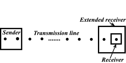
Figure 1: The communication line with the extended receiver. Using the optimized local unitary transformation of the extended receiver we increase the critical length $N_{c}$ and thus extend the creatable region in comparison with the model without the above local transformation of the extended receiver.

Further numerical simulations with the one-node receiver (justified by the theoretical arguments) show that this procedure is most effective in chains governed by the Hamiltonian with all-node interactions rather then with nearest-neighbor ones. As a result, we manage to significantly extend the creatable region and increase the mentioned above critical length up to $N_{c}=109$.

All in all, we consider the communication line based on the homogeneous spin chain with all-node interactions consisting of the following parts, Fig. 1.

1. The two node sender with an arbitrary pure state whose parameters are referred to as the control parameters (the first and the second nodes of the spin chain).

2. The one-qubit receiver whose state-parameters are referred to as the creatable parameters (the last node of the chain).

3. The two-node extended receiver consisting of the two last nodes of the chain (involving the receiver itself).

4. The transmission line connecting the sender with the extended receiver.

Our purpose is to modify the remote state creation algorithm given in ref.BZ_2015 using the optimal local unitary transformation of the extended receiver with the purpose of extending the creatable region.

The paper is organized as follows. In Sec.II, we specify the interaction Hamiltonian together with the initial condition used for the remote state creation. Sec.III is devoted to the optimization of the local unitary transformation of the extended receiver with the purpose to obtain the largest creatable region. Numerical simulations confirming the theoretical predictions are presented in Sec.IV. General conclusions are given in Sec.V.

II XY Hamiltonian and initial state of communication line

Our model of communication line is based on the homogeneous spin chain with the one-spin excitation whose dynamics is governed by the XY-Hamiltonian

$$H=\sum_{{i,j=1}\atop{j>i}}^{N}D_{ij}(I_{i,x}I_{j,x}+I_{i,y}I_{j,y}),\;\;D_{ij}=\frac{\gamma^{2}\hbar}{r^{3}_{ij}},$$ (1)

where $\gamma$ is the gyromagnetic ratio, $r_{ij}$ is the distance between the $i$th and the $j$th spins, $I_{i,\alpha}$ ($\alpha=x,y,z$) is the projection operator of the $i$th spin on the $\alpha$ axis, $D_{ij}$ is the dipole-dipole coupling constant between the $i$th and the $j$th nodes. Below we use the dimensionless time (formally setting $D_{12}=1$). Obviously, this Hamiltonian commutes with the $z$-projection of the total angular momentum $I_{z}$, so that the evolution of the one-spin excitation can be described in the $N+1$-dimensional basis (instead of the general $2^{N}$ dimensional one)

$$|{i}\rangle,\;\;i=0,\dots,N,$$ (2)

where $|i\rangle$, $i>0$, denotes the state with the $i$th excited spin, $|{0}\rangle$ corresponds to the ground state of the spin chain with zero (by convention) eigenvalue.

The general form of the initial state of the $N$-node chain with the one-excitation initial state of the two-qubit sender reads

$$|\psi_{0}\rangle=a_{0}|0\rangle+a_{1}|1\rangle+a_{2}|2\rangle,\;\;\sum_{i=0}^{2}|a_{i}|^{2}=1,$$ (3)

where the real parameter $a_{0}$ and the complex parameters $a_{1}$, $a_{2}$ are given as:

$$a_{0}=\sin\frac{\alpha_{1}\pi}{2},\;\;a_{1}=\cos\frac{\alpha_{1}\pi}{2}\cos\frac{\alpha_{2}\pi}{2}e^{2i\pi\varphi_{1}}\;\;a_{2}=\cos\frac{\alpha_{1}\pi}{2}\sin\frac{\alpha_{2}\pi}{2}e^{2i\pi\varphi_{2}},$$ (4)

$$0\leq\alpha_{i}\leq 1,\;\;\;0\leq\varphi_{i}\leq 1,\;\;\;i=1,2.$$ (5)

Note that formula (3) means that the both extended receiver and transmission line are in the ground state initially.

III Optimal local transformation of the extended receiver

In this section we derive the optimal local unitary transformation of the extended receiver which maximizes the creatable region. For this purpose we first find the general formula for the state of the extended receiver, Sec.III.1. Then we diagonalize this state using the appropriate unitary transformation $V$ and show that both non-zero eigenvalues depend on the probability of the excitation transfer to the extended receiver, Sec.III.2. After that we maximize this excitation transfer probability optimizing the control parameters, Sec.III.3. The unitary transformation $V$ corresponding to the optimized control parameters is the needed unitary transformation of the extended receiver, Sec.III.4. This is the transformation which provides the transfer of the both nonzero eigenvalues of the extended receiver to the one-node receiver. After optimization of $V$ over the time $t$ (Sec.III.5.1), we obtain the algorithm of remote state creation in Sec.III.6. It is remarkable that the optimization of the transformation $V$ can be done using the singular value decomposition of some special matrix $P$ of transition amplitudes (31) which simplifies numerical simulations. in Sec.III.5.

III.1 General state of extended receiver

As mentioned above, the state of the extended receiver is described by the density matrix reduced over all the nodes except the two last ones. Written in the basis

$$|0\rangle,\;\;|N-1\rangle,\;\;|N\rangle,\;\;|(N-1)N\rangle,$$ (6)

this state reads

$$\rho_{R_{ext}}\equiv{\mbox{Tr}}_{1,2,\dots,N-2}\rho=\left(\begin{array}[]{cccc}1-|f_{N-1}|^{2}-|f_{N}|^{2}&f_{0}f_{N-1}^{*}&f_{0}f_{N}^{*}&0\cr f_{0}^{*}f_{N-1}&|f_{N-1}|^{2}&f_{N-1}f_{N}^{*}&0\cr f_{0}^{*}f_{N}&f_{N-1}^{*}f_{N}&|f_{N}|^{2}&0\cr 0&0&0&0\end{array}\right).$$ (11)

In (6), $|(N-1)N\rangle$ means the state with the two last excited nodes of the chain, the trace is taken over the nodes $1,\dots,N-2$, the star means the complex conjugate value and $f_{N-1}$, $f_{N}$, $f_{0}$ are the transition amplitudes,

$$f_{i} = \langle i|e^{-iHt}|\Psi_{0}\rangle=R_{i}e^{2\pi i\Phi_{i}},\;\;i=0,\dots,N,$$

$$0\leq\Phi_{i}\leq 1,\;\;\;R_{i}\geq 0.$$

Remember the natural constraint

$$|f_{0}|^{2}+|f_{N}|^{2}+|f_{N-1}|^{2}\leq 1\;\;\Rightarrow\;\;R_{0}^{2}+R_{N}^{2}+R_{N-1}^{2}\leq 1,$$ (13)

where the equality corresponds to the pure state transfer to the nodes of the extended receiver because in this case $f_{i}\equiv 0$ ($0<i<N-1$).

Since the initial state is a linear function of the control parameters $a_{i}$, the transition amplitudes are also linear functions of these parameters:

$$f_{N}(t) = \langle N|e^{-iHt}|\Psi_{0}\rangle=\sum_{j=1}^{2}a_{j}\langle N|e^{-iH_{1}t}|j\rangle=\sum_{j=1}^{2}a_{j}p_{Nj}(t),$$ (14)

$$f_{0}(t) = \langle 0|e^{-iHt}|\Psi_{0}\rangle=a_{0}\equiv R_{0},$$ (15)

where $p_{kj}$ are transition amplitudes:

$$p_{kj}(t) = \langle k|e^{-iH_{1}t}|j\rangle=r_{kj}(t)e^{2\pi i\chi_{kj}(t)},\;\;k,j>0,$$

$$r_{kj}\geq 0,\;\;\;0\leq\chi_{kj}\leq 1.$$

In eq. (15), we use the fact that the ground state has zero energy by convention. We emphasize that the transition amplitudes represent the inherent characteristics of the transmission line and do not depend on the control parameters of the sender’s initial state.

III.2 Eigenvalues of extended receiver

The construction of the optimal local transformation of the extended receiver is based on the maximization of the variation intervals of the creatable eigenvalues of the density matrix $\rho_{R_{ext}}$ (11) of the extended receiver. These eigenvalues read as follows:

$$\hat{\lambda}_{\pm}=\frac{1}{2}\left(1\pm\sqrt{(1-2R^{2})^{2}+4R^{2}R_{0}^{2}}\right),$$ (17)

where we introduce the probability of the excitation transfer to the nodes of the extended receiver

$$R^{2}\equiv|f_{N-1}|^{2}+|f_{N}|^{2}=R_{N}^{2}+R_{N-1}^{2}.$$ (18)

The biggest eigenvalue $\hat{\lambda}_{+}$ as a function of $R$ and $R_{0}$ varies inside of some interval

$$\hat{\lambda}_{0}\leq\hat{\lambda}_{+}\leq 1.$$ (19)

Thus, to obtain the largest variation interval we need to minimize $\hat{\lambda}_{0}$ as a function of $R$ and $R_{0}$. It is simple to show that the minimum $\hat{\lambda}^{min}_{0}$ corresponds to $R_{0}$ =0. For this purpose we use the following substitution prompted by constraint (13):

$$R_{N}=\hat{R}_{N}\sqrt{1-R_{0}^{2}},\;\;R_{N-1}=\hat{R}_{N-1}\sqrt{1-R_{0}^{2}},\;\;\hat{R}^{2}=\hat{R}_{N}^{2}+\hat{R}_{N-1}^{2}.$$ (20)

In terms of the new notations, the largest eigenvalue reads

$$\hat{\lambda}_{+}=\frac{1}{2}\left(1+\sqrt{1-4(1-R_{0}^{2})^{2}\hat{R}^{2}(1-\hat{R}^{2})}\right)$$ (21)

Calculating the derivative of $\lambda_{+}$ with respect to $\hat{R}$ we find the extremum at $\hat{R}^{2}=\frac{1}{2}$:

$$\hat{\lambda}_{+}^{min}=\frac{1}{2}\left(1+R_{0}\sqrt{2-R_{0}^{2}}\right)$$ (22)

which is minimal at $R_{0}=a_{0}=0$:

$$\hat{\lambda}_{+}^{min}|_{R_{0}=0}=\frac{1}{2}.$$ (23)

Note that $R$ is a continuous function of the control parameters $a_{i}$, $i=1,2$, and $R=0$ at $a_{1}=a_{2}=0$. Consequently, if $R$ reaches some value $R^{opt}$, then with varying $a_{i}$, we can obtain any value of $R$ inside of the interval

$$0\leq R\leq R^{opt}.$$ (24)

The largest variation interval $0\leq R\leq 1$ corresponds to the communication line allowing the perfect state transfer of the excitation to the extended receiver. In this case the variation interval of $\lambda_{+}$ is also maximal, $\frac{1}{2}\leq\hat{\lambda}_{+}\leq 1$. However, in general, this variation interval is following:

$$1-(R^{opt})^{2}\leq\hat{\lambda}_{+}\leq 1,\;\;0\leq(R^{opt})^{2}\leq\frac{1}{2},$$ (25)

$$\frac{1}{2}\leq\hat{\lambda}_{+}\leq 1,\;\;(R^{opt})^{2}\geq\frac{1}{2}.$$

Eq.(25) shows that the interval of creatable $\hat{\lambda}_{+}$ is completely defined by the probability of the excitation transfer to the extended receiver. Therefore, the maximization of this quantity deserves the special consideration.

III.3 Control parameters maximizing $R$

The probability of the excitation transfer $R$ (18) is equal to the norm of the two-component vector $f=(f_{N-1}\;\;f_{N})^{T}$ (the superscript $T$ means transposition),

$$f=Pa,\;\;\;a=\left(\begin{array}[]{c}a_{1}\cr a_{2}\end{array}\right),\;\;\;$$ (28)

$$P=\left(\begin{array}[]{cc}p_{(N-1)1}&p_{(N-1)2}\cr p_{N1}&p_{N2}\end{array}\right)$$ (31)

Thus, the maximum $R^{opt}$ of the probability $R$ as a function of the control parameters can be found as

$$(R^{opt})^{2}=\max_{|a_{1}|^{2}+|a_{2}|^{2}=1}(|f_{N}|^{2}+|f_{N-1}|^{2}).$$ (32)

To proceed further, we write $R^{2}$ in the following form

$$R^{2}\equiv f^{+}f=a^{+}P^{+}Pa.$$ (33)

and diagonalize the matrix $P^{+}P$:

$$P^{+}P=U^{+}\Lambda_{0}^{2}U,\;\;\Lambda_{0}^{2}={\mbox{diag}}(\lambda_{-}^{2},\lambda_{+}^{2}),\;\;0\leq\lambda_{-}\leq\lambda_{+}$$ (34)

where

$$\lambda_{\pm}^{2} = \frac{1}{2}\Big{(}r_{(N-1)1}^{2}+r_{(N-1)2}^{2}+r_{N1}^{2}+r_{N2}^{2}\pm\sqrt{Q}\Big{)},$$

$$Q=(r_{(N-1)1}^{2}+r_{(N-1)2}^{2}+r_{N1}^{2}+r_{N2}^{2})^{2}-$$

$$4\Big{(}r_{(N-1)2}^{2}r_{N1}^{2}+r_{(N-1)1}^{2}r_{N2}^{2}-$$

$$2\cos(2(\chi_{(N-1)1}-\chi_{(N-1)2}-\chi_{N1}+\chi_{N2}))r_{(N-1)1}r_{(N-1)2}r_{N1}r_{N2}\Big{)},$$

So, by virtue of (34), eq.(33) reads

$$f^{+}f=b^{+}\Lambda^{2}_{0}b,\;\;b=Ua.$$ (36)

The mutual position of the eigenvalues in the matrix $\Lambda_{0}^{2}$ is taken for convenience and will be used in Sec.III.5. Now, by virtue of eq.(36), we rewrite eq.(32) as follows:

$$(R^{opt})^{2}=\max_{|b_{1}|^{2}+|b_{2}|^{2}=1}(\lambda_{-}^{2}|b_{1}|^{2}+\lambda_{+}^{2}|b_{2}|^{2}).$$ (37)

Obviously, the maximal value is achieved when $b_{2}=1$ and $b_{1}=0$:

$$(R^{opt})^{2}=\lambda_{+}^{2}.$$ (38)

The appropriate expression for the vector of control parameters $a^{opt}$ follows from the relation between $a$ and $b$ given in the second of eqs.(36):

$$Ua^{opt}=\left(\begin{array}[]{c}0\cr 1\end{array}\right),\;\;\;\Rightarrow a^{opt}=U^{+}\left(\begin{array}[]{c}0\cr 1\end{array}\right)$$ (43)

Formula (43) gives us the sender’s initial state leading to the maximal value $R^{opt}$ of the probability $R$ at a given time instant.

Note that $|f_{N-1}|=0$ at the extremum point of $|f_{N}|$ in the case of nearest neighbor approximation BZ_2015 . As a result, $R^{max}\equiv\max\limits_{|a_{1}|^{2}+|a_{2}|^{2}=1}|f_{N}|$ and there is no contribution from the $(N-1)$th node of the chain. That is why the local transformation of the two-node extended receiver is not effective in the case of nearest neighbor approximation.

III.3.1 Explicit form of $U$

We can also write the explicit form of $U$ (and, consequently, the explicit form of $a^{opt}$) in terms of the probability amplitudes $p_{ij}$. This can be done using the definition (34) written as

$$UP^{+}P=\Lambda_{0}^{2}U.$$ (44)

Let us represent the matrix $U$ in terms of the parameters $\alpha^{opt}_{i}$ and $\varphi^{opt}_{i}$:

$$U=\left(\begin{array}[]{cc}\cos\frac{\alpha^{opt}\pi}{2}&-\sin\frac{\alpha^{opt}\pi}{2}e^{-2i\varphi^{opt}}\cr\sin\frac{\alpha^{opt}\pi}{2}e^{2i\varphi^{opt}}&\cos\frac{\alpha^{opt}\pi}{2}\end{array}\right).$$ (47)

Substitute matrix (47) into eq.(44) we can solve it for the parameters $\varphi^{opt}$ and $\alpha^{opt}$:

$$\tan(\frac{\alpha^{opt}\pi}{2})=$$ (48)

$$\frac{r_{N1}^{2}+r_{(N-1)1}^{2}-\lambda_{-}}{\cos(2\pi(\phi_{12}-\chi_{(N-1)1}+\chi_{(N-1)2}))r_{(N-1)1}r_{(N-1)2}+\cos(2\pi(\phi_{12}-\chi_{N1}+\chi_{N2}))r_{N1}r_{N2}},$$

$$\tan(2\varphi^{opt}\pi)=\frac{\sin(2\pi(\chi_{(N-1)1}-\chi_{(N-1)2}))r_{(N-1)1}r_{(N-1)2}+\sin(2\pi(\chi_{N1}-\chi_{N2}))r_{N1}r_{N2}}{\cos(2\pi(\chi_{(N-1)1}-\chi_{(N-1)2}))r_{(N-1)1}r_{(N-1)2}+\cos(2\pi(\chi_{N1}-\chi_{N2}))r_{N1}r_{N2}}.$$

Then formula (43) with $U$ given by (48) gives us the expressions for the control parameters maximizing the probability $R$ of the excitation transfer to the nodes of the extended receiver.

III.4 Optimized local transformation of the extended receiver

In Sec.III.3 we find the values of the control parameters for construction of $R^{opt}$. Namely, $a_{0}=0$ (or $\alpha_{1}=0$), $\varphi_{1}$ is arbitrary, while $\alpha_{2}$ and $\varphi_{2}$ are determined by expressions (48). Now we write the explicit form of the local transformation diagonalizing the state of the extended receiver obtained for the above control parameters. Before the diagonalization, density matrix (11) reads (we mark the appropriate quantities with the superscript $opt$):

$$\rho^{opt}_{R_{ext}}\equiv{\mbox{Tr}}_{1,2,\dots,N-2}\rho=\left(\begin{array}[]{cccc}1-(R^{opt})^{2}&0&0&0\cr 0&|f^{opt}_{N-1}|^{2}&f^{opt}_{N-1}(f^{opt}_{N})^{*}&0\cr 0&(f^{opt}_{N-1})^{*}f^{opt}_{N}&|f^{opt}_{N}|^{2}&0\cr 0&0&0&0\end{array}\right).$$ (53)

It is remarkable that the central nonzero $2\times 2$ block of the density matrix $\rho^{opt}_{R_{ext}}$ can be factorized as

$$\left(\begin{array}[]{cc}|f^{opt}_{N-1}|^{2}&f^{opt}_{N-1}(f^{opt}_{N})^{*}\cr(f^{opt}_{N-1})^{*}f^{opt}_{N}&|f^{opt}_{N}|^{2}\end{array}\right)=ff^{+}.$$ (56)

It is clear that this block can be diagonalized by the matrix $V_{0}$ of the following form:

$$V_{0}=\frac{1}{R^{opt}}\left(\begin{array}[]{cc}\displaystyle f^{opt}_{N}&-f^{opt}_{N-1}\cr(f^{opt}_{N-1})^{*}&(f^{opt}_{N})^{*}\end{array}\right)$$ (59)

with the eigenvalue matrix

$$\Lambda_{b}={\mbox{diag}}(0,(R^{opt})^{2}),$$ (60)

so that we can write

$$\rho^{opt}_{R_{ext}}=V^{+}\Lambda V,$$ (61)

where

$$V={\mbox{diag}}(1,V_{0},1),\;\;$$ (62)

$$\Lambda={\mbox{diag}}(1-(R^{opt})^{2},\Lambda_{b},0).$$ (63)

Consequently, applying the unitary transformation $V$ (62) to $\rho^{opt}_{R_{ext}}$ we obtain the diagonal density matrix

$$\tilde{\rho}^{opt}_{R_{ext}}=V\rho^{opt}_{R_{ext}}V^{+}=\Lambda.$$ (64)

The transformation (62) with $V_{0}$ from (59) is the needed local unitary transformation of the extended receiver.

III.4.1 The optimized state of one-qubit receiver

To obtain the optimized state of the receiver, we reduce the density matrix (64) to the state of the last node using the basis (6). Owing to the mutual positions of the eigenvalues in the diagonal matrix (63), this state reads:

$$\rho^{opt}_{R}={\mbox{diag}}(1-(R^{opt})^{2},(R^{opt})^{2}).$$ (65)

Thus the both non-zero eigenvalues are transferred from the extended receiver to the receiver itself.

III.5 Singular value decomposition of $P$ in terms of matrices $V^{+}_{0}$, $U$ and $\Lambda_{0}$

It is remarkable that the matrices $V_{0}$, $U$ and $\Lambda_{0}$ can be given another meaning. In fact, the central $2\times 2$ block of eq.(64) by virtue of eqs.(59,60,62,63) yields

$$V_{0}ff^{+}V_{0}^{+}=(R^{opt})^{2}\left(\begin{array}[]{cc}0&0\cr 0&1\end{array}\right).$$ (68)

On the other hand, eq.(33) by virtue of eq.(34) can be written in the form

$$f^{+}f=a^{+}U^{+}\Lambda_{0}\tilde{V}\tilde{V}^{+}\Lambda_{0}Ua,$$ (69)

where $\tilde{V}$ is some unitary matrix. Now we can formally split eq. (69) into equation for $f$

$$f = \tilde{V}^{+}\Lambda_{0}Ua\;\;\Rightarrow\;\;$$ (70)

$$\tilde{V}f = \Lambda_{0}Ua\stackrel{{\scriptstyle(\ref{a})}}{{=}}\left(\begin{array}[]{c}0\cr\lambda_{+}\end{array}\right)$$ (73)

and its Hermitian conjugate. Multiplying eq.(73) by its Hermitian conjugation from the right we obtain

$$\tilde{V}ff^{+}\tilde{V}^{+}=\lambda_{+}^{2}\left(\begin{array}[]{cc}0&0\cr 0&1\end{array}\right).$$ (76)

Comparison of eqs. (68) and (76) prompts us to identify

$$\tilde{V}=V_{0},\;\;R_{opt}^{2}=\lambda_{+}^{2}.$$ (77)

Comparing eq.(73) with eq.(28) for $f$ by virtue of eqs.(77) we conclude that

$$P=V^{+}_{0}\Lambda_{0}U,$$ (78)

i.e., the matrices $V^{+}_{0}$, $U$ and $\Lambda$ constructed in Secs. III.3 and III.4 represent the singular value decomposition of the matrix $P$. This fact allows us to simplify the algorithm of the numerical construction and time-optimization of the probability $R^{opt}$ together with the unitary transformations $V$ and $U$. This algorithm reads as follows.

1. Calculate the matrix $P$ as a function of the time $t$ for the given Hamiltonian governing the spin dynamics and calculate its largest singular value $\lambda_{+}$ as a function of the time $t$.

2. Find the time instant $t_{0}$ maximizing the largest singular value of the matrix $P$. This maximal singular value gives the maximized probability

   $$(R^{(max)})^{2}\equiv(R^{(opt)})^{2}|_{t=t_{0}}=(\lambda_{+})^{2}|_{t=t_{0}}.$$ (79)

3. Construct the singular decomposition of $P$ at the time instant $t=t_{0}$ obtaining the matrices $U^{max}$ (the optimized unitary transformation of the sender) and $V^{max}$ (the optimized unitary transformation of the extended receiver):

   $$V^{max}=V|_{t=t_{0}},\;\;\;U^{max}=U|_{t=t_{0}}.$$ (80)

Especially important in the above algorithm is the time-optimization of the probability $R^{opt}$ in no.2 which is given the special consideration in the next paragraph.

III.5.1 Time-maximization of probability $(R^{opt})^{2}$

In this subsection we give some remarks regarding the maximization of the largest singular value $\lambda_{+}$ (or the probability $(R^{opt})^{2}$) as a function of time. The probability $(R^{opt})^{2}$ is an oscillating function of the time $t$ with the well defined first maximum BZ_2015 . The value of this maximum $(R^{max})^{2}$ together with the corresponding time instant $t_{0}$ as functions of the chain length are shown in Fig.2.

Figure 2: (a) The maximal excitation transfer probability $(R^{max})^{2}$ and (b) the corresponding time instant $t_{0}$ as functions of the chain length $N$ in different models based on the homogeneous spin-1/2 chain with XY-Hamiltonian: nearest neighbor approximation (the dash-line), all-node interactions without the local transformation of the extended receiver (the lower solid line), all-node interactions involving the optimal local transformation of the extended receiver (the upper solid line). The upper and lower horizontal dot-lines indicate, respectively, the lower limit of the high-probability state transfer ($(R^{max})^{2}=0.9$) and the minimal value of $(R^{max})^{2}=\frac{1}{2}$ providing the creation of any eigenvalue ($\frac{1}{2}\leq\lambda_{max}\leq 1$) in the receiver’s state. In all cases $t_{0}$ is essentially a linear function of $N$, note that the line corresponding to the model with all-node interactions involving the local transformation $V$ is a bit below the line corresponding to the model without $V$ (although these two lines are indistinguishable in the figure).

For comparison, $(R^{max})^{2}$ as function of $N$ for the state creation without the local transformation of the extended receiver is shown for both nearest-neighbor approximation (the dash-line, $(R^{max})^{2}=|f_{N}|^{2}$ in this case) and all-node interaction (the lower solid line). We see that the high probability state transfer ($(R^{max})^{2}\geq 0.9$) is possible if $N\leq 6$, $N\leq 4$ and $N\leq 17$ in the models, respectively, with nearest-neighbor interactions, with all-node interactions without the optimized unitary transformation $V$ and involving this transformation.

Another parameter indicated in Fig.2 is the critical length $N_{c}$ such that any eigenvalue can be created in the receiver if $N\leq N_{c}$. We see that the excitation transfer probability exceeds the critical value $R^{2}_{c}=\frac{1}{2}$ if $N\leq 34$, $N\leq 37$ and $N\leq 109$ in the models, respectively, with nearest-neighbor interactions, with all-node interactions without the optimized unitary transformation $V$ and involving this transformation.

III.6 The algorithm of remote state creation. Analysis of creatable region

As the main result of this section we formulate the complete algorithm of the remote state creation.

1. Construct the optimized unitary transformations $U^{max}$ and $V^{max}$ and the optimal time instant $t_{0}$ using the algorithm in Sec.III.5.

2. Create the initial state (3) of the whole chain (i.e. the one-excitation pure state of the sender and the ground state of the rest of the chain).

3. Apply the unitary transformation $U^{max}$ (80) to the sender.

4. Switch on the evolution of the spin chain.

5. Apply the local unitary transformation $V^{max}$ to the extended receiver at the time instant $t_{0}$.

6. Determine the state of the receiver at the time instant $t=t_{0}$ as the trace of the whole density matrix over the all nodes except the receiver’s node. The resulting density matrix reads as follows (we use the basis $|0\rangle$, $|N\rangle$):

   $$\rho_{R}={\mbox{Tr}}_{N-1}\left[V^{max}\rho_{R_{ext}}(V^{max})^{+}\right]=\left(\begin{array}[]{cc}1-|z|^{2}&f_{0}z\cr f_{0}z^{*}&|z|^{2}\end{array}\right),\;\;\;$$ (83)

   $$z=\frac{1}{R^{max}}(f_{N}^{*}f^{max}_{N}+f_{N-1}^{*}f^{max}_{N-1})=R_{z}e^{2i\Phi_{z}\pi}.$$ (84)

This matrix coincides with $\rho^{opt}_{R}$ (65) if we use optimized initial state (43) with $f_{0}=0$ at the step no.2. The function $z$ in eq.(83) is nothing but the transition amplitude to the last node (compare with ref. BZ_2015 ) after the evolution followed by the local optimal transformation $V^{max}$ (don’t mix $z$ with $f_{N}$!). We see that the probability of the excitation transfer to the last node $|z|^{2}$ reaches its maximal value $|z_{max}|^{2}=(R^{max})^{2}$ for the optimal initial state (43) and is the sum of probabilities $|f_{N-1}^{max}|^{2}$ and $|f_{N}^{max}|^{2}$. The latter statement is the consequence of the optimizing transformation $V^{max}$. Without this transformation, we would have just $|z_{max}|^{2}=|f_{N}^{max}|^{2}$. Thus, again, the probability of the excitation transfer to the receiver of the communication line is the parameter responsible for the area of the creatable region in the state-space of the receiver BZ_2015 . We emphasize that our model allows us to increase the length of the high probability ($\geq 90\%$) state transfer through the homogeneous spin chain from $N=6$ nodes (nearest neighbor approximation) to $N=17$, see Fig.2.

Analyzing the creatable region we follow ref.BZ_2015 and use the eigenvalue-eigenvector parametrization of the receiver state:

$$\rho^{B}=U^{B}\Lambda^{B}(U^{B})^{+},$$ (85)

where $\Lambda^{B}$ is the diagonal matrix of eigenvalues and $U^{B}$ is the matrix of eigenvectors:

$$\Lambda^{B}={\mbox{diag}}(\lambda,1-\lambda),$$ (86)

$$U^{B}=\left(\begin{array}[]{cc}\cos\frac{\beta_{1}\pi}{2}&-e^{-2i\beta_{2}\pi}\sin\frac{\beta_{1}\pi}{2}\cr e^{2i\beta_{2}\pi}\sin\frac{\beta_{1}\pi}{2}&\cos\frac{\beta_{1}\pi}{2}\end{array}\right).$$ (89)

In the ideal case, varying $\lambda$ and $\beta_{i}$ ($i=1,2$) inside of the intervals

$$\frac{1}{2}\leq\lambda\leq 1,$$ (90)

$$0\leq\beta_{i}\leq 1,\;\;i=1,2,$$ (91)

we can create the whole state-space of the receiver. However, the parameters $\lambda$ and $\beta_{i}$ are not arbitrary because they depend on the control parameters via the functions $R_{0}$, $R_{z}$ and $\Phi_{z}$ in accordance with the formulas BZ_2015 :

$$\lambda = \frac{1}{2}\left(1+\sqrt{(1-2R_{z}^{2})^{2}+4R_{z}^{2}R_{0}^{2}}\right),$$ (92)

$$\cos\beta_{1}\pi = \frac{1-2R_{z}^{2}}{\sqrt{(1-2R_{z}^{2})^{2}+4R_{z}^{2}R_{0}^{2}}},\;\;\Rightarrow$$ (93)

$$\beta_{1}\pi = \arccos\frac{1-2R_{z}^{2}}{\sqrt{(1-2R_{z}^{2})^{2}+4R_{z}^{2}R_{0}^{2}}},$$ (94)

$$\beta_{2} = \Phi_{z}.$$ (95)

As a result, the variation intervals of the creatable parameters $\lambda$ and $\beta_{1}$ become restricted so that the creatable region does not cover the whole state space of the receiver. On the contrary, any value of $\beta_{2}$ can be constructed by the proper choice of the phases $\varphi_{i}$, $i=1,2$ in the initial state (3) BZ_2015 . This conclusion follows from the explicit expression for $z$ in (84). Therefore, below we consider the simplified map

$$(\alpha_{1},\alpha_{2})\to(\lambda,\beta_{1}).$$ (96)

IV Numerical simulations

Now we apply the algorithm proposed in Sec.III.6 to the numerical study of map (96) in the case of spin chain of the critical length $N_{c}=109$. In Fig.3, we collect the results of such simulations for the different models shown in Fig.2: the model with all-node interactions involving the optimized local transformation of the extended receiver ($V=V^{max}$), Fig.3a; the model with all-node interactions without the optimized local transformation of the extended receiver ($V$ equals the identity matrix $I$), Fig.3b; the model with nearest neighbor interactions, Fig.3c. We see that using the all-node interaction without optimized local transformation we can only slightly extend the creatable region (compare Figs. 3b and 3c), while the optimized transformation $V^{max}$ allows us to significantly extend it, see Fig.3a. Results of our numerical simulations confirm the theoretical predictions of Sec.III regarding the extension of the creatable region.

Figure 3: The creatable regions in the state-space of the receiver for the different models based on the homogeneous spin-1/2 chain and XY-Hamiltonian. (a) The model with all-node interactions involving the optimal local transformation $V^{max}$ of the extended receiver; (b)The model with all-node interactions without the local transformation $V^{max}$ of the extended receiver; (c) The model with nearest neighbor interactions. Solid- and dash-lines correspond to $\alpha_{1}=const$ and $\alpha_{2}=const$ respectively; the interval between the neighboring lines is $0.1$

V Conclusions

In this paper we show that an effective method of increasing the both distance of the high probability state transfer and creatable region is the specially constructed local unitary transformation applied at the receiver side of the chain. This local transformation must involve not only the nodes of the receiver itself, but also some nodes from the close neighborhood. In our case of the one-node receiver we involve only the one additional node which (together with the node of the receiver) form the two-node extended receiver. We emphasize that this procedure (which uses the two-qubit extended receiver) is not effective in the case of nearest neighbor approximation and becomes useful if the spin dynamics is governed by the all node interaction Hamiltonian, which, obviously, is more natural in the case of dipole-dipole interactions.

As a result, we increase the distance of the high probability ($\geq 90\%$) state transfer from $N=6$ (nearest neighbor approximation) to $N=17$. The chain length allowing us to create any eigenvalue of the receiver is increased from $N_{c}=34$ (nearest neighbor approximation) to $N_{c}=109$, as shown in Fig.2. As a consequence, the creatable region is also extended.

The algorithm constructing the optimized unitary transformation of the extended receiver $V^{max}$ is described in Sec.III in detail. Doing this we also obtain the initial sender’s state ($a^{opt}$ in eq.(43) with $U=U^{max}$) maximizing the excitation transfer probability. It is remarkable that the optimized unitary transformation of the extended receiver $V^{max}$ can be constructed in terms of the transition amplitudes $p_{ij}$ ($i=1,2$, $j=N-1,N$) between the nodes of the sender and extended receiver (amplitudes $p_{ij}$ are inherent characteristics of the communication line). More exactly, this transformation can be obtained from the singular value decomposition of the matrix $P$ (31) whose elements are the above probabilities. This observation is very useful for the numerical simulation of the remote state creation. Results of such simulations are shown in Fig.3.

The work is partially supported by RFBR (grant 15-07-07928). A.I.Z. is partially supported by DAAD (the Funding program ”Research Stays for University Academics and Scientists”, 2015 (50015559))

References

- (1) N.A.Peters, J.T.Barreiro, M.E.Goggin, T.-C.Wei, and P.G.Kwiat, Phys.Rev.Lett. 94, 150502 (2005)
- (2) N.A.Peters, J.T.Barreiro, M.E.Goggin, T.-C.Wei, and P.G.Kwiat in Quantum Communications and Quantum Imaging III, ed. R.E.Meyers, Ya.Shih, Proc. of SPIE 5893 (SPIE, Bellingham, WA, 2005)
- (3) B.Dakic, Ya.O.Lipp, X.Ma, M.Ringbauer, S.Kropatschek, S.Barz, T.Paterek, V.Vedral, A.Zeilinger, C.Brukner, and P.Walther, Nat. Phys. 8, 666 (2012).
- (4) G.Y. Xiang, J.Li, B.Yu, and G.C.Guo Phys. Rev. A 72, 012315 (2005)
- (5) S.Pouyandeh, F. Shahbazi, A. Bayat, Phys.Rev.A 90, 012337 (2014)
- (6) C.H.Bennett, G.Brassard, C.Crépeau, R.Jozsa, A.Peres, and W.K.Wootters, Phys. Rev. Lett. 70, 1895 (1993)
- (7) B.Yurke, D.Stoler, Phys. Rev. A 46, 2229 (1992)
- (8) B.Yurke, D.Stoler, Phys. Rev. Lett. 68, 1251 (1992)
- (9) M.Zukowski, A.Zeilinger, M.A.Horne, A.K.Ekert, Phys. Rev. Lett. 71, 4287 (1993)
- (10) D.Bouwmeester, J.-W. Pan, K.Mattle, M.Eibl, H.Weinfurter, and A. Zeilinger, Nature 390, 575 (1997)
- (11) D. Boschi, S. Branca, F. De Martini, L. Hardy, and S. Popescu, Phys. Rev. Lett. 80, 1121 (1998)
- (12) S. Bose, Phys. Rev. Lett. 91, 207901 (2003)
- (13) M.Christandl, N.Datta, A.Ekert and A.J.Landahl, Phys.Rev.Lett. 92, 187902 (2004)
- (14) C.Albanese, M.Christandl, N.Datta and A.Ekert, Phys.Rev.Lett. 93, 230502 (2004)
- (15) P.Karbach and J.Stolze, Phys.Rev.A 72, 030301(R) (2005)
- (16) G.Gualdi, V.Kostak, I.Marzoli and P.Tombesi, Phys.Rev. A 78, 022325 (2008)
- (17) A.Wójcik, T.Luczak, P.Kurzyński, A.Grudka, T.Gdala, and M.Bednarska Phys. Rev. A 72, 034303 (2005)
- (18) G. De Chiara, D. Rossini, S. Montangero, R. Fazio, Phys. Rev. A 72, 012323 (2005)
- (19) A. Zwick, G.A. Álvarez, J. Stolze, O. Osenda, Phys. Rev. A 84, 022311 (2011)
- (20) A. Zwick, G.A. Álvarez, J. Stolze, O. Osenda, Phys. Rev. A 85, 012318 (2012)
- (21) A. Zwick, G.A. Álvarez, J. Stolze, O Osenda, Quant. Inf. Comput. 15, 582 (2015)
- (22) J.Stolze, G. A. Álvarez, O. Osenda, A. Zwick in Quantum State Transfer and Network Engineering. Quantum Science and Technology, ed. by G.M.Nikolopoulos and I.Jex, Springer Berlin Heidelberg, Berlin, p.149 (2014)
- (23) E.I.Kuznetsova and A.I.Zenchuk, Phys.Lett.A 372, pp.6134-6140 (2008)
- (24) G.M.Nikolopoulos and I.Jex, eds., Quantum State Transfer and Network Engineering, Series in Quantum Science and Technology, Springer, Berlin Heidelberg (2014)
- (25) A. Bayat and V. Karimipour Phys.Rev.A 71, 042330 (2005)
- (26) P. Cappellaro, Phys.Rev.A 83, 032304 (2011)
- (27) W. Qin, Ch. Wang, G. L. Long, Phys.Rev.A 87, 012339 (2013)
- (28) A.Bayat, Phys. Rev. A 89, 062302 (2014)
- (29) C. Godsil, S. Kirkland, S. Severini, Ja. Smith Phys. Rev. Lett. 109, 050502 (2012)
- (30) R.Sousa, Ya. Omar, New J. Phys. 16, 123003 (2014).
- (31) D. Burgarth and S. Bose, Phys.Rev.A 71, 052315 (2005)
- (32) K. Shizume, K. Jacobs, D. Burgarth, and S. Bose, Phys. Rev. A 75, 062328 (2007)
- (33) P. Lorenz, J. Stolze, Phys. Rev. A 90, 044301 (2014)
- (34) L.Banchi, A. Bayat, P. Verrucchi, and S.Bose, Phys.Rev.Let. 106, 140501 (2011)
- (35) A.I.Zenchuk, Phys. Rev. A 90, 052302(13) (2014)
- (36) G. A. Bochkin and A. I. Zenchuk, Phys.Rev.A 91, 062326(11) (2015)
- (37) A.I.Zenchuk, J. Phys. A: Math. Theor. 45 (2012) 115306
- (38) S. Pouyandeh, F. Shahbazi, Int. J. Quantum Inform. 13, 1550030 (2015)
- (39) S.Yang, A. Bayat, S. Bose, Phys.Rev.A 84, 020302 (2011)