QM/MM DESCRIPTION OF PERIODIC SYSTEMS

Abstract

A QM/MM implementation for periodic systems is reported. This is done for the case of molecules and for systems with two and three-dimensional periodicity, which is suitable to model electrolytes in contact with electrodes. Tests on different water-containing systems, ranging from the water dimer up to liquid water indicate the correctness of the scheme. Furthermore, molecular dynamics simulations are performed, as a possible direction to study realistic systems.

1 Introduction

The theoretical description of extended systems has become more and more important in the course of treating realistic systems. Presently, energy conversion has become an important topic, and there has been an upsurge of research in electrochemistry.

The targeted systems are rather complex, e.g. the simulation of electrolytes in contact with electrodes. This can often not be done with density functional theory, due to the system size and corresponding large numerical effort. On the other hand, empirical models may not always work well, and besides, they depend on the choice of parameters, such as force fields. The combination of quantum mechanical (QM) and molecular mechanics (MM) methods (QM/MM) is therefore tempting in this area. Therefore, the present article aims at a description of an implementation of such a QM/MM scheme for molecular and periodic systems.

2 Method

The main intention is to establish a QM/MM scheme for molecules and periodic systems. These schemes have become popular over the past years especially for the modeling of biological systems, see e.g. [1, 2, 3, 4, 5]. Also, periodic systems are now investigated on this level, e.g. [6, 7, 8, 9]. The systems to be targeted with the present approach are in the area of electrochemistry, e.g. electrolytes, in contact with metal surfaces. Motivated by the aim to develop a theoretical scheme to treat electrochemical interfaces self-consistently, we formulated a QM/MM approach which in the first stage is making use of the so called subtractive scheme to evaluate the system’s energy (see, e.g. [5]). In this scheme, the total energy and forces are obtained as

$$E_{\mbox{QM/MM}}^{\mbox{whole system}}= E_{\mbox{MM}}^{\mbox{whole system}}+E_{\mbox{QM}}^{\mbox{QM region}}-E_{\mbox{MM}}^{\mbox{QM region}}$$ (1)

$$\vec{F}_{\mbox{QM/MM}}^{\mbox{whole system}}= \vec{F}_{\mbox{MM}}^{\mbox{whole system}}+\vec{F}_{\mbox{QM}}^{\mbox{QM region}}-\vec{F}_{\mbox{MM}}^{\mbox{QM region}}$$ (2)

Compared to molecules, the periodicity has to be taken into account. This is in the present approach achieved by summing the interactions with the help of the Ewald method in the case of periodicitiy in three dimensions, and Parry’s potential [10] for the case of periodicity in two dimensions. The MM interaction is thus summed for the whole system, and subsequently corrected due to the contributions from the QM region: the energy of the QM region and its periodic replicas are again summed with the Ewald or Parry method, on the MM and the QM level separately. Subsequently, the data obtained is inserted in equations 1 and 2. This QM/MM level corresponds to a mechanical embedding, where the interactions between the QM and MM region are treated on the MM level. The QM and MM calculations for the QM region are performed without taking the atoms into account which are not in the QM region. However, the total energy in equation 1 and the forces in equation 2 now include effects of the QM region. An extension of mechanical embedding leads to electrostatic embedding where the QM calculations include the effects of all the other atoms by e.g. representing these atoms by point charges. The present implementation corresponds thus to a periodic extension of a mechanical embedding. For a comparison of the embedding schemes, see e.g. [11].

3 Implementation

The present scheme requires a QM and an MM code, and a connection between both. For the MM region GULP was used [12], and for the QM region CRYSTAL [13]. Energies and gradients are obtained from these codes and manipulated according to equations (1) and (2). Besides these codes, it is necessary to have a routine which works with the manipulated energies and forces: here, a modified version of GULP is used. Finally, an interface (i.e. wrapper) to perform the communication between the three aforementioned codes is required, for purposes such as e.g. extracting the energy and gradients, or setting up new input files during an optimisation (e.g. GULP and CRYSTAL inputs for the QM region are generated automatically during an optimisation).

This strategy has the advantage that features which are available within GULP can be used for QM/MM calculations, such as the geometry optimisation or molecular dynamics. However, one has to keep in mind that in the present implementation only the MM Hessian is available.

4 Computational parameters

The target of the present work is mainly to establish the methodology. A relatively simple potential is used [14], which employs intermolecular Coulomb and Lennard-Jones terms, and a harmonic intramolecular potential. The advantage is that this is well suited for test purposes, as e.g. results for the water dimer already exist and can thus be compared with. The ab-initio calculations were done on the simple LDA (local density approximation) level, with Dirac-Slater exchange and the correlation functional as in Ref. [15]. If not stated otherwise, for oxygen a $[4s3p]$ Gaussian basis set (as in Ref. [16]), and for hydrogen a $[2s1p]$ basis set (as in Ref. [17]) was used. These basis sets are medium sized, which also means that they are robust and problems from linear dependencies are unlikely to occur.

The structures are visualised with XCrysDen [18] and Molden [19].

5 Results and discussion

5.1 Structural optimisation

5.1.1 Water molecule and dimer

Results for the geometry and vibrational frequencies of the water molecule are displayed in table 1. The MM results are practically identical to those of the publication where this potential was suggested [14]. The QM results (on the LDA level) are in reasonable agreement with the LDA results in Ref. [20]. Larger basis sets were used in Ref. [20], and indeed, the agreement of the computed H-O-H angle (108.1^∘ vs 104.9^∘ in Ref. [20]) can be improved, when the oxygen basis set is enhanced. For this purpose, the $[4s3p2d]$ oxygen basis set from Ref. [21] was used, together with a finer integration grid and higher thresholds for the integral selection. The O-H distance agrees already well with the medium sized basis sets described in section 4. With the enhanced basis set, also the vibrational frequencies agree well with the ones computed in Ref. [20].

Table 1: Geometry of the H₂O molecule, vibrational frequencies and charges at the MM level calculated with the empirical potential and with QM on LDA-level. For the MM system, charges are as defined by the potential, while Mulliken charges are given for the QM case.

property	MM	QM	QM (enhanced basis set)	Ref. [20] (LDA)
distance O-H1 (O-H2 is equal)	1.000 Å	0.971 Å	0.971 Å	0.970 Å
distance H1-H2	1.633 Å	1.572 Å	1.542 Å
angle H1-O-H2	109.5∘	108.1∘	105.1∘	104.9∘
frequencies	1653	1436	1566	1560
in cm-1	3822	3675	3712	3729
	3952	3837	3826	3835
charge O	-0.82 $|e|$	-0.60 $|e|$	-0.65 $|e|$
charge H1,H2	0.41 $|e|$	0.30 $|e|$	0.33 $|e|$
total energy, in $E_{h}$	0	-75.8763	-75.8883

There are many studies on the equilibrium geometry of the water dimer, e.g. based on Møller-Plesset perturbation theory [22, 23], with a local correlation treatment [25], coupled cluster methods [26, 27] or density functional theory [28]. Numerous model potentials have been developed, see for example Ref. [29]. For results on the water dimer with the model used in the present work, see Ref. [30], and for an overview of results with model potentials, see Ref. [31].

The optimisation at the MM [12] and QM [32, 33, 34] level is routine and can be done with the codes used. The QM/MM level is more challenging due to the lack of the QM Hessian, and thus various possibilities for the optimisation of a (H₂O)₂ dimer were tested. Most successful turned out to be the Broyden-Fletcher-Goldfarb-Shanno (BFGS) or Davidon-Fletcher-Powell (DFP) optimiser in combination with the force minimisation option, which means that the gradient norm is the quantity to be minimised, instead of the energy. The conjugate gradient minimisation in combination with force minimisation also worked, but needed many more iterations.

Structural parameters for the (H₂O)₂ dimer are displayed in table 2. In this dimer, as displayed in figure 1, the right H₂O is considered as the QM region.

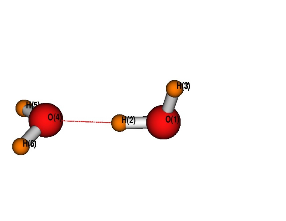
Figure 1: (Colour online) MM equilibrium geometry of the water dimer. Oxygen is displayed as a big red sphere. The QM/MM equilibrium geometry is similar. The hydrogen atom H(2) is in the latter two cases below (’below’ according to the arrangement in the figure) the O-O-axis, whereas in the case of the QM geometry, the hydrogen is above the O-O axis.

Table 2: Geometry of the (H₂O)₂ dimer, with the empirical potential (MM), with QM at the LDA-level and at the QM/MM level. The labels of the atoms are as in figure 1, and O1, H2, H3 is the QM region.

property	MM	QM	QM/MM
distance O1-H2	1.017 Å	0.993 Å	0.990 Å
distance O1-H3	0.999 Å	0.970 Å	0.971 Å
distance O1-O4	2.738 Å	2.651 Å	2.753 Å
distance O4-H5 (O4-H6 is equal)	1.003 Å	0.972 Å	1.003 Å
angle H2-O1-H3	107.6∘	108.8∘	105.2∘
angle H5-O4-H6	108.5∘	109.7∘	108.5∘
angle O1-H2-O4	176.1∘	(360-174.9)∘	175.1∘
total energy, in $E_{h}$	-0.0109	-151.7732	-75.8866

The MM results for the dimer are in full agreement with an earlier work where the same potential was used [30], which can be seen as a test of the implementation of the potential (the computed MM oxygen-oxygen equilibrium distance in [30] is 2.737 Å, and the computed MM intermolecular energy is 28.63 kJ/mol, corresponding to 0.0109 $E_{h}$ or 0.30 eV). The QM results show that there is a stronger attraction on this level, resulting in a shorter oxygen-oxygen equilibrium bond length. The results agree reasonably well with the LDA results from [20], where an oxygen-oxygen equilibrium distance of 2.710 Å was obtained and a binding energy of 9.02 kcal/mol, corresponding to 0.39 eV or 0.0144 $E_{h}$. Using data from tables 2 and 1 to compute the binding energy, then the binding energy would be 0.0206 $E_{h}$ or 0.56 eV; the deviations are again due to the smaller basis sets used in the present work. The MM value (0.0109 $E_{h}$, 0.30 eV, see above) is close to the experiment [35], whereas LDA overbinds. The QM/MM results are very similar to the MM results for the molecule made of O4, H5, H6, i.e. the molecule which is not in the QM region. This is to be expected, as the QM part mainly influences the molecule in the QM region, and the intermolecular interactions are due to the MM part. The QM part has thus only an indirect influence due to the slightly different geometry of the QM water molecule. Thus, the oxygen-oxygen equilibrium distance obtained with the QM/MM approach is close to the MM value.

Subsequently, the energy curve when separating both water molecules was computed. For this purpose, the oxygen-oxygen distance was fixed at a certain value, and the geometries of all hydrogen positions were optimised. This way, one point of the potential curve is obtained. When this procedure is performed for a set of oxygen-oxygen distances, then the potential curve in figure 2 is obtained. There, the data was fitted with a Morse potential. It turns out that MM and QM/MM are very similar (equilibrium distance, curvature at the minimum, binding energy of the dimer). This is due to the reason mentioned above, that the QM part has only little influence on the intermolecular interaction. From the fits with the Morse potential, the binding energy is obtained as 0.22 eV (MM), 0.21 eV (QM/MM) versus 0.55 eV (QM).

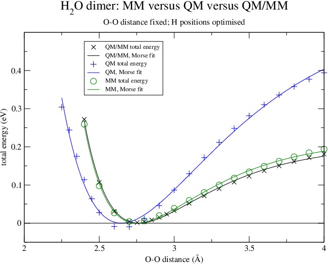
Figure 2: (Colour online) The total energy for a water dimer, on the level of MM, QM and QM/MM. All hydrogen positions are optimised for a fixed oxygen distance, and the potential curve is obtained as a function of the oxygen-oxygen distance. The minimum energy of the various fits is shifted to zero.

5.1.2 Two dimensional periodicity

In a next step, periodicity was implemented. An advantage of the presently used codes is that both employ the same electrostatic potentials, i.e. Saunders’ potential [36] for one dimensional periodicity, Parry’s [10] for two dimensional periodicity and the Ewald potential for three dimensional periodicity. Note that in the present case of two-dimensional periodicity, the implementation of the periodicity is truly two-dimensional. This implies that the system is not repeated in the third direction (z-direction), and there is consequently no parameter for the vacuum thickness.

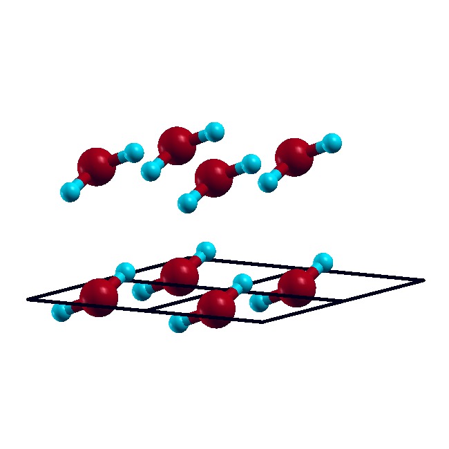
Figure 3: (Colour online) A periodic arrangement of a water dimer, with lattice constant a=b (in the present figure: a=b=3 Å) and a fixed angle $\gamma=90^{\circ}$. Note that the system is periodic only in two dimensions, but not in the z-direction.

As a test, the potential curve was computed, where a water dimer was periodically arranged, with the lattice constants $a=b$, and a fixed angle $\gamma=90^{\circ}$ (see figure 3). Then, the oxygen positions were fixed at a distance of 2.8 Å (one oxygen 2.8 Å vertically above the other along the z-axis, which is the non-periodic direction). For various lattice constants, the hydrogen positions were optimised. In the QM/MM case, one molecule was considered the QM region; here it is the one whose oxygen atom has a hydrogen bridge to the second water molecule. This resulted in three potential curves visualised in figure 4.

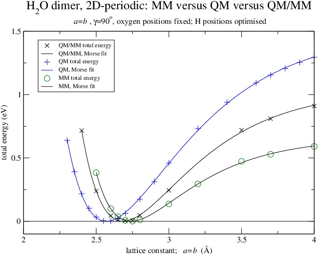
Figure 4: (Colour online) The total energy for a water dimer, arranged with two-dimensional periodicity, on the level of MM, QM and QM/MM. All hydrogen positions are optimised for fixed oxygen positions, and the potential curve is obtained as a function of the lattice constant, with the lattice constant a=b and a fixed angle $\gamma=90^{\circ}$. The minimum energy of the various fits is shifted to zero.

For large values of the lattice constant, one obtains essentially the structure of a single water dimer, as the interaction between the dimers is small. When reducing the lattice constant, the water molecules tilt to the molecules of the neighbouring cell, as the interaction to this neighbouring molecule becomes more important. The potential curve has a minimum for a certain lattice constant, which is shortest at the QM level and longer at the MM level. The QM/MM equilibrium distance is now in between the QM and MM equilibrium distance, as the dominant interactions are now the QM-interaction between neighbouring molecules in one layer and the MM-interaction between neighbouring molecules in the other layer.

5.2 Molecular dynamics

In a next step, the QM/MM expressions as in equations (1) and (2) were used to perform molecular dynamics. The implementation is similar to the one used for geometry optimisation as was described in the previous sections. The energy and gradient calculations in the molecular dynamics part of the GULP code were correspondingly modified, and the ab-initio energy and gradient are again extracted from CRYSTAL.

5.2.1 Water dimer

To test the implementation, molecular dynamics simulations were performed for the water dimer (without any periodicity), at the level of MM, QM and QM/MM. The starting point was a system consisting of two water molecules at a relatively large distance (oxygen-oxygen distance $\sim$5 Å). At the MM level, as CPU time is not critical, a simple, nearly brute force way to obtain the minimum structure was to employ an NVT ensemble at $T$=10 K with a production run of 400 ps, using a time step of 1 fs.

On the QM level, the optimisation was more difficult due to problems with overheating, when the system gained kinetic energy too quickly. Thus, a series of molecular dynamics runs was used to obtain the minimum structure. Starting again from the geometry where two water molecules are far apart, a 1 ps simulation was performed (time step 1 fs, initial temperature 100 K, and cooling with a rate of 0.1 K/step down to 5 K). Subsequently, the final geometry was used as a new initial geometry, and a simulation at a temperature of 5 K (NVE ensemble, 1 ps, time step 1 fs) was performed. After repeating this procedure a few times, the final structure was essentially the one of the geometry optimisation in table 1.

At the QM/MM level, the simulation turned out to be straightforward. The NVT ensemble was used, at a temperature of 10 K, and with a simulation length of 100 ps (1 fs time step).

In all cases, the final structure agreed reasonably well with the one obtained from a straightforward optimisation as described in section 5.1, e.g. the O-O distance at the end of the MD run was 2.733 Å (MM), 2.614 Å (QM), and 2.781 Å (QM/MM).

5.2.2 Two-dimensional periodicity

Two water molecules were periodically arranged in a two-dimensional box of 5$\times$5 Å size, and a molecular dynamics run at the MM level was performed (NVT ensemble, 400 ps total length, 1 fs time step). The initial temperature was 300 K, and lowered to 50 K in 25000 steps. The final structure agreed with the one obtained by a normal minimisation with the default optimiser (BFGS). With a similar (though shorter) molecular dynamics run and using the QM/MM energy and forces, an optimisation at the QM/MM level was performed. The structure agreed reasonably well with the one from the MM optimisation. This serves as an additional test for the QM/MM implementation.

5.2.3 Three-dimensional periodicity

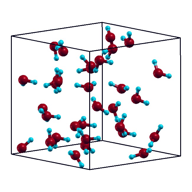
Figure 5: (Colour online) A snapshot of the molecular dynamics simulation of a box containing 32 water molecules.

In the case of three-dimensional periodicity, 32 water molecules were considered, in a cubic box of 9.856 Å, corresponding to a density of 1 g/cm³ (see figure 5). The calculation of the radial pair distribution function and of the mean square displacement (MSD) was implemented in GULP, or independently computed with ISAACS [37]. A simulation length of 25 ps equilibration (NVT ensemble) and subsequently 100 ps production was chosen (NVE ensemble), at a time step of 1 fs.

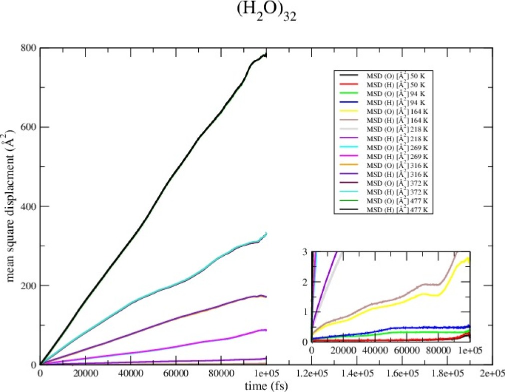
Figure 6: (Colour online) The mean square displacement (MSD) for a system of 32 H₂O molecules, at the MM level, for temperatures in the range from 50 to 491 K. The MSD for temperatures $\lesssim$ 164 K is almost constant and displayed in the inset.

Results for the MSD at the MM level are summarised in figure 6. The temperature is the one as it was obtained as an average over the run. For temperatures $\gtrsim$ 218 K, there is a linear slope, which increases with temperature, whereas for temperatures $\lesssim$ 164 K, the MSD is approximately constant. This indicates a phase transition from the liquid to the solid phase in this temperature range, with this potential. The radial pair distribution functions are displayed in figure 7. They agree reasonably well with the literature, e.g. with empirical potentials [38, 39, 40], DFT [41, 42, 43] and recently also MP2 [44].

a)          

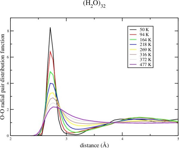
b)          

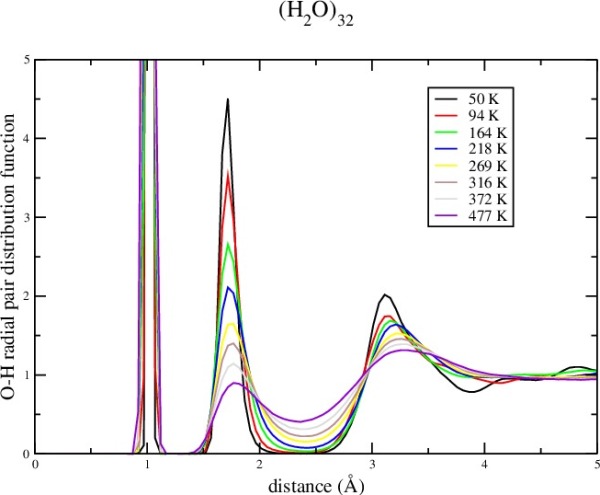
c)          

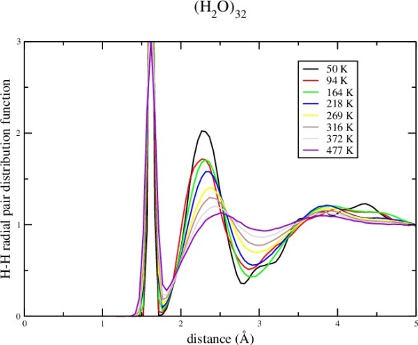
Figure 7: (Colour online) The radial pair distribution function for a system of 32 H₂O molecules, at the MM level, for temperatures in the range from 50 to 477 K. The displayed radial pair distribution functions are for O-O (a), O-H (b) and H-H (c).

Finally, QM/MM simulations were performed for systems with 32 H₂O molecules, out of which 0 to 4 molecules were treated on the QM level, and all the other ones on the MM level. This is labelled as (H₂O)${}^{n}_{32-n}$ (where superscript and subscript are the numbers of QM and MM treated molecules, respectively), with $n$ ranging from 0 to 4. The QM region is fixed to the initially defined QM molecules. More sophisticated approaches define a spatial QM region, and consider diffusion into and out of this region via an adaptive scheme [45, 46]. The present results are similar to the MM results, for example a comparison is shown in figure 8 for the oxygen-oxygen radial pair distribution function. In the simulations, it turns out that QM clusters are formed: initially, the QM molecules were put far apart. After a while, they start to form dimers in the case of (H₂O)${}_{30}^{2}$, and arrange in a triangle for (H₂O)${}_{29}^{3}$. For (H₂O)${}_{28}^{4}$, there are enough QM molecules so that they can form a chain, which connects the cells; i.e. there is a stripe of QM molecules going through the unit cell. This formation of QM clusters and QM stripes is presumably due to the different binding energies of QM molecules and MM molecules with the functional and potential used in the present work (see the discussion about the water dimer in section 5.1.1). This may require a readjustment of the water potential is some cases, but not necessarily in general. For example, in the case of systems such as water in contact with a transition metal surface, the first water layer has an ice-like structure, and might constitute a possible QM region, whereas the remaining water molecules might be described with a semi-empirical potential.

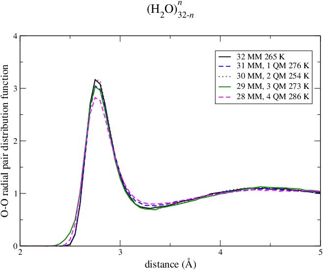
Figure 8: (Colour online) The radial pair distribution function for a system of 32 H₂O molecules, at the QM/MM level, with the number of QM molecules varied from 0 to 4.

6 Conclusion

A QM/MM implementation for periodic systems has been presented. Calculations on the water dimer and for water with two and three-dimensional periodicity show that the implementation works properly. Structural optimisation and molecular dynamics simulations have been implemented on the QM/MM level. In the case of three-dimensional periodicity, as a test system a box of 32 water molecules was studied at the MM and QM/MM level. The pair distribution functions agree well when computed on the MM or QM/MM levels.

References

- [1] F. Maseras and K. Morokuma, J. Comput. Chem. 16:1170-1179 (1995).
- [2] M. Svensson, S. Humbel, R. D. J. Froese, T. Matsubara, S. Sieber, and K. Morokuma, J. Phys. Chem. 100:19357-19363 (1996).
- [3] U. Eichler, C. M. Kölmel, and J. Sauer, J. Comput. Chem. 18:463-477 (1996).
- [4] D. Bakowies and W. Thiel, J. Phys. Chem. 100:10580-10594 (1996).
- [5] P. Sherwood et al, J. Mol. Struct. (Theochem) 632:1-28 (2003).
- [6] J. Sauer and M. Sierka, J. Comput. Chem. 21:1470-1493 (2000).
- [7] D. A. Yarne, M. E. Tuckerman, and G. J. Martyna, J. Chem. Phys. 115:3531-3539 (2001).
- [8] T. Laino, F. Mohamed, A. Laio, and M. Parrinello, J. Chem. Theory Comput. 2:1370-1378 (2006).
- [9] C. F. Sanz-Navarro, R. Grima, A. García, E. A. Bea, A. Soba, J. M. Cela, P. Ordejón, Theor. Chem. Acc. 128:825-833 (2011).
- [10] D. E. Parry, Surf. Science 49:433-440 (1975); 54, 195 (1976) (Erratum).
- [11] H. Lin and D. G. Truhlar, Theor. Chem. Acc. 117:185-199 (2007).
- [12] J. D. Gale, J. Chem. Soc., Faraday Trans. 93:629-637 (1997).
- [13] R. Dovesi, V. R. Saunders, C. Roetti, R. Orlando, C. M. Zicovich-Wilson, F. Pascale, B. Civalleri, K. Doll, N. M. Harrison, I. J. Bush, Ph. D’Arco, M. Llunell, CRYSTAL2009, University of Torino, Torino, 2009.
- [14] K. Toukan and A. Rahman, Phys. Rev. B 31:2643-2648 (1985).
- [15] J. P. Perdew and A. Zunger, Phys. Rev. B 23:5048-5079 (1981).
- [16] M.D. Towler, N.L. Allan, N.M. Harrison, V.R. Saunders, W.C. Mackrodt and E. Aprà, Phys. Rev. B 50:5041-5054 (1994).
- [17] R. Ditchfield, W. J. Hehre, and J. A. Pople, J. Chem. Phys. 54:724-728 (1971).
- [18] A. Kokalj, Comp. Mater. Sci. 28:155-168 (2003).
- [19] G. Schaftenaar and J. H. Noordik, J. Comput.-Aided Mol. Design, 14:123-134 (2000).
- [20] X. Xu and W. A. Goddard III, J. Phys. Chem. A 108:2305-2313 (2004).
- [21] L. Valenzano, F. J. Torres A., K. Doll, F. Pascale, C. M. Zicovich-Wilson and R. Dovesi, Z. Phys. Chem. 220:893-912 (2006).
- [22] B. J. Smith, D. J. Swanton, J. A. Pople, H. F. Schafer III, and L. Radom, J. Chem. Phys. 92:1240-1247 (1990).
- [23] M. Schütz, S. Brdarski, P.-O. Widmark, R. Lindh, and G. Karlström, J. Chem. Phys. 107:4597-4605 (1997).
- [24] K. S. Kim, B. J. Mhin, U-S. Choi, and K. Lee, J. Chem. Phys. 97:6649-6662 (1992).
- [25] M. Schütz, G. Rauhut, and H.-J. Werner, J. Phys. Chem. A 102:5997-6003 (1998)
- [26] W. Klopper, J. G. C. M. van Duijneveldt-van de Rijdt and F. B. van Duijneveldt, Phys. Chem. Chem. Phys. 2:2227-2234 (2000).
- [27] G. S. Tschumper, M. L. Leininger, B. C. Hoffman, E. F. Valeev, H. F. Schaefer, and M. Quack, J. Chem. Phys. 116:690-701 (2002).
- [28] J. A. Anderson and G. S. Tschumper, J. Phys. Chem. A 110:7268-7271 (2006).
- [29] W. L. Jorgensen, J. Am. Chem. Soc. 103:335-340 (1981).
- [30] P. T. Kiss and A. Baranyai, J. Chem. Phys. 131:204310 (2009).
- [31] H. Yu and W. van Gunsteren, J. Chem. Phys. 121:9549-9564 (2004).
- [32] K. Doll, V. R. Saunders, N. M. Harrison, Int. J. Quantum Chem. 82:1-13 (2001).
- [33] K. Doll, Comp. Phys. Comm. 137:74-88 (2001).
- [34] B. Civalleri, Ph. D’Arco, R. Orlando, V. R. Saunders, and R. Dovesi, Chem. Phys. Lett. 348:131-138 (2001).
- [35] L. A. Curtiss, D. J. Frurip, and M. Blander, J. Chem. Phys. 71:2703-2711 (1979).
- [36] V. R. Saunders, C. Freyria-Fava, R. Dovesi, and C. Roetti, Comp. Phys. Comm. 84:156-172 (1994).
- [37] S. Le Roux and V. Petkov, J. Appl. Cryst. 43:181-185 (2010).
- [38] A. Rahman and F. H. Stillinger, J. Chem. Phys. 55:3336-3359 (1971).
- [39] W. L. Jorgensen, J. Chandrasekhar, J. D. Madura, R. W. Impey, and M. L. Klein, J. Chem. Phys. 79:926-935 (1983).
- [40] M. Sprik, J. Phys. Chem. 95:2283-2291 (1991).
- [41] K. Laasonen, M. Sprik, M. Parrinello, and R. Car, J. Chem. Phys,. 99:9080-9089 (1993).
- [42] S. Izvekov and G. A. Voth, J. Chem. Phys. 116:10372-10376 (2002).
- [43] J. VandeVondele, F. Mohamed, M. Krack, J. Hutter, M. Sprik, and M. Parrinello, J. Chem. Phys. 122:014515 (2005).
- [44] M. Del Ben, M. Schönherr, J. Hutter, and J. VandeVondele, J. Phys. Chem. Lett. 4:3753-3759 (2013).
- [45] R. E. Bulo, B. Ensing, J. Sikkema, and L. Visscher, J. Chem. Theory Comput. 5:2212-2221 (2009).
- [46] R. E. Bulo, C. Michel, P. Fleurat-Lessard, and Ph. Sautet, J. Chem. Theory Comput. 9:5567-5577 (2013).