On the $b$-functions of hypergeometric systems

Abstract.

For any integer $d\times(n+1)$ matrix $A$ and parameter $\beta\in\mathbb{C}^{d}$ let $M_{A}(\beta)$ be the associated $A$-hypergeometric (or GKZ) system in the variables $x_{0},\ldots,x_{n}$. We describe bounds for the (roots of the) $b$-functions of both $M_{A}(\beta)$ and its Fourier transform along the hyperplanes $(x_{j}=0)$. We also give an estimate for the $b$-function for restricting $M_{A}(\beta)$ to a generic point.

Let $D$ be the ring of algebraic $\mathbb{C}$-linear differential operators on $\mathbb{C}^{n+1}$ with coordinates $x_{0},\ldots,x_{n}$.

Definition 0.1 (Compare [Kas77, MM04]).

Let $M$ be a left $D$-module and pick an element $m\in M$ with annihilator $I\subseteq D$. If $(V^{i}D)$ is the vector space spanned by the monomials $x^{\alpha}\partial^{\beta}$ with $\alpha_{0}-\beta_{0}\geq i$ then the $b$-function of $m\in M$ along the coordinate hyperplane $x_{0}=0$ is the minimal monic polynomial $b(s)$ that satisfies: $b(x_{0}\partial_{0})\cdot m\in(V^{1}D)\cdot m$ in $M$, which is to say $b(x_{0}\partial_{0})\in I+(V^{1}D)$ in $D$.

If $M$ is cyclic, i.e., $M=D/I$, then we call $b$-function of $M$ the $b$-function in the above sense of the element $1+I\in M$.

The $b$-function exists in greater generality along any hypersurface $(f=0)$, as long as the module $M$ is holonomic, cf. [Kas77]. The $V$-filtration of Kashiwara and Malgrange then takes the form $(V^{i}D)=\{P\in D\mid f^{i+k}\text{ divides }P\bullet f^{k}\text{ for }k\gg 0\}$. Both the $V$-filtration and the $b$-function are intimately connected to the restriction of the given $D$-module to the hypersurface. The purpose of this note is to give, for any $A$-hypergeometric system as well as its Fourier transform, an explicit arithmetic description of a bound for the root set of the $b$-function along any coordinate hyperplane that involves the parameter $\beta$ in a very elementary way.

We have several applications in mind: first, it is a longstanding question to understand the monodromy of $A$-hypergeometric systems, and for this purpose the roots of the $b$-function as considered above can be of some use. On the other hand, the Fourier transform of an $A$-hypergeometric system often (see [SW09b]) appears as a direct image module under a natural torus embedding given by the columns of the matrix $A$. This point of view turns out to be extremely useful for Hodge theoretic considerations of $A$-hypergeometric systems (see [Rei14]). It is one of the fundamental insights of Morihiko Saito (see [Sai88, Section 3.2]) that the boundary behavior of variations of Hodge structures (or, more generally, of mixed Hodge modules) is controlled by the Kashiwara–Malgrange filtration along such a boundary divisor. In the case of a cyclic $D$-module, such as $A$-hypergeometric systems or their Fourier transforms, one can often deduce a large part of this filtration from the values of the $b$-function. We refer to [RS15] for an immediate application of our results. In a third direction, one can also see our calculation of the $b$-function of the Fourier transform as a refinement of [SW09b, FFW11] geared towards restriction of $A$-hypergeometric systems.

In the last part we compute an upper bound for the $b$-function of restriction of the $A$-hypergeometric system to a generic point, again in elementary terms of $A$ and $\beta$. Since the restriction of a $D$-module to a point is a dual object to the $0$-th level solution functor, our estimate can be viewed as a step towards a sheafification in $\beta$ of the solution space, a problem that remains unsolved.

Acknowledgements

We would like to thank the Forschungsinstitut Oberwolfach for hosting us in April of 2015.

We are greatly indebted to an unknown referee for very careful reading, pointing out a number of misprints.

1. Basic notions and results

Notation.

Throughout, the base field is $\mathbb{C}$ and we consider a $\mathbb{C}$-vector space $V$ of dimension $n+1$.

In this introductory section we review basic facts on $A$-hypergeometric systems as well as the Euler–Koszul functor. Readers are advised to refer to [MMW05] for more detailed explanations.

Notation 1.1.

For any integer matrix $A$, let $R_{A}$ (resp. $O_{A}$) be the polynomial ring over $\mathbb{C}$ generated by the variables $\partial_{j}$ (resp. $x_{j}$) corresponding to the columns ${\mathbf{a}}_{j}$ of $A$. We identify $O_{A}$ with the symmetric algebra on $\operatorname{Hom}_{\mathbb{C}}(V,\mathbb{C})\cong\bigoplus\mathbb{C}\cdot x_{j}$. Further, let $D_{A}$ be the ring of $\mathbb{C}$-linear differential operators on $O_{A}$, where we identify $\frac{\partial}{\partial x_{j}}$ with $\partial_{j}$ and multiplication by $x_{j}$ with $x_{j}$ so that both $R_{A}$ and $O_{A}$ become subrings of $D_{A}$.

1.1. $A$-hypergeometric systems

Let $A=({\mathbf{a}}_{0},\ldots,{\mathbf{a}}_{n})$ be an integer $d\times(n+1)$ matrix, $d\leq n+1$. For convenience we assume that $\mathbb{Z}A=\mathbb{Z}^{d}$. For $(v_{1},\ldots,v_{r})={\mathbf{v}}\in\mathbb{Z}^{r}$ we denote by ${\mathbf{v}}_{+},{\mathbf{v}}_{-}$ the vectors given by

$$({\mathbf{v}}_{+})_{j}=\max(0,v_{j})\qquad\text{and}\qquad({\mathbf{v}}_{-})_{j}=\max(0,-v_{j}).$$

For the complex parameter vector $\beta\in\mathbb{C}^{d}$ consider the system of $d$ homogeneity equations

(1.1) $$E_{i}\bullet\phi = \beta_{i}\cdot\phi,$$

where $E_{i}=\sum_{j=0}^{n}a_{i,j}x_{j}\partial_{j}$ is the $i$-th Euler operator, together with the toric (partial differential) equations

(1.2) $$\{(\underbrace{\partial^{{\mathbf{v}}_{+}}-\partial^{{\mathbf{v}}_{-}}}_{:=\Delta_{\mathbf{v}}})\bullet\phi=0 \mid A\cdot{\mathbf{v}}=0\}.$$

In $R_{A}$, the toric operators $\{\Delta_{\mathbf{v}}|A\cdot{\mathbf{v}}=0\}$ generate the toric ideal $I_{A}$. The quotient

$$S_{A}:=R_{A}/I_{A}$$

is naturally isomorphic to the semigroup ring $\mathbb{C}[\mathbb{N}A]$. In $D_{A}$, the left ideal generated by all equations (1.1) and (1.2) is the hypergeometric ideal $H_{A}(\beta)$. We put

$$M_{A}(\beta):=D_{A}/H_{A}(\beta);$$

this is the $A$-hypergeometric system introduced and first investigated by Gelfand, Graev, Kapranov, and Zelevinsky, in [Gel86] and a string of other papers. $\diamond$

1.2. $A$-degrees

If the rowspan of $A$ contains ${\mathbf{1}}_{A}$ we call $A$ homogeneous. Homogeneity is equivalent to $I_{A}$ defining a projective variety, and also to the system $H_{A}(\beta)$ having only regular singularities [Hot98, SW08]. A more general $A$-degree function on $R_{A}$ and $D_{A}$ is induced by:

$$-\deg_{A}(x_{j}):={\mathbf{a}}_{j}=:\deg_{A}(\partial_{j}).$$

We denote $\deg_{A,i}(-)$ the $A$-degree function associated to the weight given by the $i$-th row of $A$, so $\deg_{A}=(\deg_{A,1},\ldots,\deg_{A,d})$.

An $R_{A}$- (resp. $D_{A}$-)module $M$ is $A$-graded if it has a decomposition $M=\bigoplus_{\alpha\in\mathbb{Z}^{d}}M_{\alpha}$ such that the module structure respects the grading $\deg_{A}(-)$ on $R_{A}$ (resp. $D_{A}$) and $M$. If $N$ is an $A$-graded $R_{A}$-module, then we denote $\deg_{A}(N)\subseteq\mathbb{Z}^{d}$ the set of all degrees of all non-zero homogeneous elements of $N$. The quasi-degrees $\operatorname{qdeg}_{A}(N)$ of $N$ are the points in the Zariski closure in $\mathbb{C}^{d}$ of $\deg_{A}(N)$.

As is common, if $M$ is $A$-graded then $M({\mathbf{b}})$ denotes for each ${\mathbf{b}}\in\mathbb{Z}A$ its shift with graded structure $(M({\mathbf{b}}))_{{\mathbf{b}}^{\prime}}=M_{{\mathbf{b}}+{\mathbf{b}}^{\prime}}$.

1.3. Euler–Koszul complex

Since

$$x^{\mathbf{u}}E_{i}-E_{i}x^{\mathbf{u}} = -(A\cdot{\mathbf{u}})_{i}x^{\mathbf{u}},$$

$$\partial^{\mathbf{u}}E_{i}-E_{i}\partial^{\mathbf{u}} = (A\cdot{\mathbf{u}})_{i}\partial^{\mathbf{u}},$$

we have

(1.3) $$E_{i}P=P(E_{i}-\deg_{A,i}(P))$$

for any $A$-homogeneous $P\in D_{A}$ and all $i$.

On the $A$-graded $D_{A}$-module $M$ one can thus define commuting $D_{A}$-linear endomorphisms $E_{i}$ via

$$E_{i}\circ m:=(E_{i}+\deg_{A,i}(m))\cdot m$$

for $A$-homogeneous elements $m\in M$. In particular, if $N$ is an $A$-graded $R_{A}$-module one obtains commuting sets of $D_{A}$-endomorphisms on the left $D_{A}$-module $D_{A}\otimes_{R_{A}}N$ by

$$E_{i}\circ(P\otimes Q):=(E_{i}+\deg_{A,i}(P)+\deg_{A,i}(Q))P\otimes Q.$$

The Euler–Koszul complex $\mathscr{K}_{\bullet}(N;\beta)$ of the $A$-graded $R_{A}$-module $N$ is the homological Koszul complex induced by $E-\beta:=\{(E_{i}-\beta_{i})\circ\}_{1}^{d}$ on $D_{A}\otimes_{R_{A}}N$. In particular, the terminal module $D_{A}\otimes_{R_{A}}N$ sits in homological degree zero. We denote the homology groups of $\mathscr{K}_{\bullet}(N;\beta)$ by $\mathscr{H}_{\bullet}(N;\beta)$. Implicit in the notation is “$A$”: different presentations of semigroup rings that act on $N$ yield different Euler–Koszul complexes.

If $N({\mathbf{b}})$ denotes the usual shift-of-degree functor on the category of graded $R_{A}$-modules, then $\mathscr{K}_{\bullet}(N;\beta)({\mathbf{b}})$ and $\mathscr{K}_{\bullet}(N({\mathbf{b}});\beta-{\mathbf{b}})$ are identical.

1.4. The toric category

There is a bijection between faces $\tau$ of the cone $\mathbb{R}_{\geq 0}A$ and $A$-graded prime ideals $I_{A}^{\tau}=I_{A}+R_{A}\{\partial_{j}\mid j\not\in\tau\}$ of $R_{A}$ containing $I_{A}$. If the origin is a face of $\mathbb{R}_{\geq 0}A$, it corresponds to the ideal $I^{\emptyset}_{A}=(\partial_{0},\ldots,\partial_{n})$. In general, $R_{A}/I_{A}^{\tau}\cong\mathbb{C}[\mathbb{N}\tau]$.

An $R_{A}$-module $N$ is toric if it is $A$-graded and has a (finite) $A$-graded composition chain

$$0=N_{0}\subsetneq N_{1}\subsetneq N_{2}\cdots\subsetneq N_{k}=N$$

such that each composition factor $N_{i}/N_{i-1}$ is isomorphic as $A$-graded $R_{A}$-module to an $A$-graded shift $(R_{A}/I_{A}^{\tau})({\mathbf{b}})$ for some ${\mathbf{b}}\in\mathbb{Z}A$ and some face $\tau$. The category of toric modules is closed under the formation of subquotients and extensions.

For toric input $N$, the modules $\mathscr{H}_{\bullet}(N;\beta)$ are holonomic. As $D_{A}$ is $R_{A}$-free, any short exact sequence $0\longrightarrow N^{\prime}\longrightarrow N\longrightarrow N^{\prime\prime}\longrightarrow 0$ of $A$-graded $R_{A}$-modules produces a long exact sequence of Euler–Koszul homology. If $\beta$ is not a quasi-degree of $N$ then the complex $\mathscr{K}_{\bullet}(N;\beta)$ is exact, and if $N$ is a maximal Cohen–Macaulay module then $\mathscr{K}_{\bullet}(N;\beta)$ is a a resolution of $\mathscr{H}_{0}(N;\beta)$.

1.5. The Euler space

Notation 1.2.

The $\mathbb{C}$-linear span of the Euler operators $\{E_{i}\}_{1}^{d}$ is called the Euler space. Let $E$ be in the Euler space. Then $E$ is in a unique fashion (as $\operatorname{rk}(A)=d$) a linear combination $E=\sum c_{i}E_{i}$. With $\beta_{E}:=\sum c_{i}\beta_{i}$ we have $E-\beta_{E}\in H_{A}(\beta)$. We further write $\deg_{E}(-)$ for the degree function $\sum c_{i}\deg_{A,i}(-)$.

Denote $\theta_{j}=x_{j}\partial_{j}$ and $\theta=(\theta_{0},\ldots,\theta_{n})$. A linear combination $\sum_{j}v_{j}\theta_{j}$ is in the Euler space if and only if the coefficient vector ${\mathbf{v}}=(v_{0},\ldots,v_{n})$, interpreted as a linear functional on $\mathbb{C}^{n+1}$ via ${\mathbf{v}}((q_{0},\ldots,q_{n})):=\sum v_{i}q_{i}$, is the pull-back via $A$ of a linear functional on $\mathbb{C}^{d}$. In other words,

$$[{\mathbf{v}}\cdot\theta^{T}=\sum_{j}v_{j}\theta_{j}\text{ is in the Euler space}]\Leftrightarrow[{\mathbf{v}}={\mathbf{c}}\cdot A\text{ for some }{\mathbf{c}}\in\mathbb{C}^{d}].$$

If $L\colon\mathbb{C}^{d}\longrightarrow\mathbb{C}$ is a linear functional then the Euler operator in $H_{A}(\beta)$ corresponding to its image under $\operatorname{Hom}_{\mathbb{C}}(\mathbb{C}^{d},\mathbb{C})\stackrel{{\scriptstyle\cdot A}}{{\longrightarrow}}\operatorname{Hom}_{\mathbb{C}}(\mathbb{C}^{n+1},\mathbb{C})$ is denoted $E_{L}-\beta_{L}$.

Lemma 1.3.

For any set $F$ of columns of $A$ contained in a hyperplane that passes through the origin of $\mathbb{C}^{d}$ but does not contain ${\mathbf{a}}_{k}$, there is an Euler operator $E_{F}-\beta_{F}$ in $H_{A}(\beta)$ such that the coefficient of $\theta_{j}$ in $E_{F}$ is zero for all $j\in F$, and equal to $1$ for $j=k$. If $\mathbb{R}_{\geq 0}F$ is a facet of $\mathbb{R}_{\geq 0}A$ then $E_{F}-\beta_{F}$ is unique.

Proof.

Choose for any such set $F$ a linear functional $L\colon\mathbb{Q}^{d}\longrightarrow\mathbb{Q}$ that vanishes on $F$ while $L({\mathbf{a}}_{k})=1$. The corresponding Euler operator $E_{L}-\beta_{L}$ has the desired properties, and if we define numbers $a_{L,j}$ by

$$E_{L}=:\sum_{j}a_{L,j}x_{j}\partial_{j}$$

then $a_{L,j}=L({\mathbf{a}}_{j})$. The uniqueness in the facet case is obvious. ∎

2. Restricting the Fourier transform

The Fourier transform $\mathscr{F}(-)$ is a functor from the category of $D$-modules on $V$ to the category of $D$-modules on the dual space $V^{*}=\operatorname{Hom}_{\mathbb{C}}(V,\mathbb{C})$. In this section we bound the $b$-function along a coordinate hyperplane of the Fourier transform $\mathscr{F}(M_{A}(\beta))$ of the hypergeometric system. Note that this module is called $\check{M}^{\beta}_{A}$ in [RS15].

The square of the Fourier transform is the involution induced by $x\mapsto-x$, which has no effect on the analytic properties of the modules we study. In particular, $b$-functions along coordinate hyperplanes are unaffected by this involution and we therefore consider $\mathscr{F}^{-1}(M_{A}(\beta))$ without harm.

We start with introducing some notation.

Notation 2.1.

Let $\{y_{j}\}$ be the coordinates on $V^{*}$ such that $\mathscr{F}^{-1}(\partial_{j})=y_{j}$ on the level of differential operators. We let $\tilde{D}_{A}$ be the ring of $\mathbb{C}$-linear differential operators on $\tilde{O}_{A}:=\mathbb{C}[y_{0},\ldots,y_{n}]$, generated by $\{y_{j},\delta_{j}\}_{0}^{n}$ where $\delta_{j}$ denotes $\frac{\partial}{\partial y_{j}}$. Then $\mathscr{F}^{-1}(x_{j})=-\delta_{j}$. The subring $\mathbb{C}[\delta_{1},\ldots,\delta_{n}]$ of $\tilde{D}_{A}$ is denoted $\tilde{R}_{A}$. The isomorphism $(\tilde{-})\colon D_{A}\longrightarrow\tilde{D}_{A}$ induced by $\tilde{\partial}_{j}:=y_{j}$ and $\tilde{x}_{j}=\delta_{j}$ sends $O_{A}$ to $\tilde{R}_{A}$ and $R_{A}$ to $\tilde{O}_{A}$.

Thus, $\tilde{I}_{A}:=\mathscr{F}^{-1}(I_{A})$ is an ideal of $\tilde{O}_{A}$; the advantage of considering $\mathscr{F}^{-1}$ rather than $\mathscr{F}$ is that $\tilde{I}_{A}$ retains the shape of the generators of $I_{A}$ as differences of monomials. For each $j$ set $\tilde{\theta}_{j}:=\mathscr{F}^{-1}(\theta_{j})=-\delta_{j}y_{j}$. The $i$-th level $V$-filtration on $\tilde{D}_{A}$ along $y_{t}$ is spanned by $\delta^{\alpha}y^{\beta}$ with $\beta_{t}-\alpha_{t}\geq i$.

Before we get into the technical part, let us show by example an outline of what is to happen.

Example 2.2.

Let $A=\begin{pmatrix}-1&0&1\\ 1&1&1\end{pmatrix}$, a matrix whose associated semigroup ring is a normal complete intersection. We will estimate the $b$-function for restriction to the hyperplane $y_{1}=0$ (corresponding to the middle column) of $\mathscr{F}^{-1}(M_{A}(\beta))$.

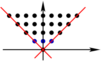
Figure 1. Restriction of the Fourier transform to $y_{1}=0$.

The ideal $\tilde{H}_{A}(\beta):=\mathscr{F}^{-1}(H_{A}(\beta))$ is generated by

(2.1) $$-\tilde{\theta}_{0}+\tilde{\theta}_{2}-\beta_{1},\qquad\tilde{\theta}_{0}+\tilde{\theta}_{1}+\tilde{\theta}_{2}-\beta_{2},\qquad y_{0}y_{2}-y_{1}^{2}.$$

Since $y_{1}\in(V^{1}\tilde{D}_{A})$, $y_{0}y_{2}$ and hence also $\tilde{\theta}_{0}\tilde{\theta}_{2}$ are in $(V^{1}\tilde{D}_{A})+\tilde{H}_{A}(\beta)$. The strategy of the example, and of the theorem in this section, is to multiply the element $1\in\tilde{D}_{A}$ by suitable Euler operators so that the result is a sum of a polynomial $p(\tilde{\theta}_{1})$ with an element of $\mathbb{C}[\tilde{\theta}_{0},\tilde{\theta}_{1},\tilde{\theta}_{2}]\cdot\tilde{\theta}_{0}\tilde{\theta}_{2}$; this certifies $p(\tilde{\theta}_{1})$ to be in $\tilde{H}_{A}(\beta)+(V^{1}\tilde{D}_{A})$.

In the case at hand, the relevant Euler operators are $2\tilde{\theta}_{0}+\tilde{\theta}_{1}+\beta_{1}-\beta_{2}$ and $\tilde{\theta}_{1}+2\tilde{\theta}_{2}-\beta_{1}-\beta_{2}$. Modulo $\tilde{H}_{A}(\beta)$ we can rewrite $(V^{1}\tilde{D}_{A})\ni 4\delta_{0}\delta_{2}y_{1}^{2}\equiv 4\tilde{\theta}_{0}\tilde{\theta}_{2}\equiv(-\tilde{\theta}_{1}-\beta_{1}+\beta_{2})(-\tilde{\theta}_{1}+\beta_{1}+\beta_{2})$. It follows that $(\tilde{s}+\beta_{1}-\beta_{2})(\tilde{s}-\beta_{1}-\beta_{2})$ is a multiple of the $b$-function, where $\tilde{s}=\tilde{\theta}_{1}=-y_{1}\delta_{1}-1$. This Fourier twist in the argument of the $b$-function occurs naturally throughout and we will make our computations in this section in terms of $b(\tilde{s})$.

The expressions $\tilde{\theta}_{1}+2\tilde{\theta}_{2}$ and $2\tilde{\theta}_{0}+\tilde{\theta}_{1}$ that appear in the Euler operators we used can be found systematically as follows. Let $d_{1},d_{2}$ denote the coordinates on the degree group $\mathbb{Z}^{2}$ corresponding to $E_{1}$ and $E_{2}$; compare the discussion following Notation 1.2. An element of $S_{A}$ has degree on the facet $\mathbb{R}_{\geq 0}{\mathbf{a}}_{0}$ if and only if the functional $L_{1}(d_{1},d_{2})=d_{1}+d_{2}$ vanishes, and the Euler field that corresponds to this functional in the spirit of Lemma 1.3 is exactly $\theta_{1}+2\theta_{2}-\beta_{1}-\beta_{2}$. The elements of $S_{A}$ with degree on the facet $\mathbb{R}_{\geq 0}{\mathbf{a}}_{2}$ are determined by the vanishing of $L_{2}(d_{1},d_{2})=d_{2}-d_{1}$ and the Euler field corresponding to this functional is exactly $2\theta_{0}+\theta_{1}+\beta_{1}-\beta_{2}$. It is no coincidence that the union of the kernels of these two functionals is exactly the set of quasi-degrees of $S_{A}/\partial_{1}\cdot S_{A}$. The point is that modulo $\tilde{H}_{A}(\beta)$ all monomials in $\tilde{S}_{A}$ with degree in $\mathbb{R}_{+}A$ are already in $(V^{1}\tilde{D}_{A})$. The task is then to deal with those with degree on the boundary through multiplication with suitable expressions.

The picture shows in blue the elements of $A$, in black the other elements of $\mathbb{N}A$, and in red the quasi-degrees of $S_{A}/\partial_{1}\cdot S_{A}$. Note finally that $(\beta_{2}-\beta_{1}){\mathbf{a}}_{1}$ and $(\beta_{1}+\beta_{2}){\mathbf{a}}_{1}$ are the intersections of $\mathbb{R}\cdot{\mathbf{a}}_{1}$ with $\operatorname{qdeg}_{A}(S_{A})+\beta$.

We now generalize the computation of the example to the general case.

Convention 2.3.

For the remainder of this section we consider restriction to the hyperplane $y_{0}$ in order to save overhead (in terms of a further index variable).

Consider the toric module $N=S_{A}/\partial_{0}S_{A}$, and take a toric filtration

$$(N)\qquad\qquad\qquad\qquad\qquad\qquad\qquad\qquad\qquad 0=N_{0}\subsetneq N_{1}\subsetneq\ldots\subsetneq N_{k}=N\qquad\qquad\qquad\qquad\qquad\qquad\qquad$$

with composition factors

$$\overline{N}_{\alpha}:=N_{\alpha}/N_{\alpha-1},$$

each isomorphic to some shifted face ring $S_{F^{\prime}_{\alpha}}({\mathbf{b}}_{\alpha})$, $F^{\prime}_{\alpha}=\tau_{\alpha}\cap A$, attached to a face $\tau_{\alpha}$ of $\mathbb{R}_{\geq 0}A$. (We will call such $F^{\prime}_{\alpha}$ also a face.) Lifting the $N_{\alpha}$ to $S_{A}$ yields an increasing sequence of $A$-graded ideals $J_{\alpha}\ni\partial_{0}$ of $S_{A}$ with $N_{\alpha}=J_{\alpha}/\partial_{0}\cdot S_{A}$.

Choose for each composition factor a facet $F_{\alpha}$ containing $F^{\prime}_{\alpha}$. Note that none of the faces $F^{\prime}_{\alpha}$ will contain ${\mathbf{a}}_{0}$ (as $\partial_{0}$ is zero on $N$ but not nilpotent on any face ring of a face containing ${\mathbf{a}}_{0}$) and hence we can arrange that the corresponding facets do not contain ${\mathbf{a}}_{0}$ either.

Lemma 1.3 produces for each $\overline{N}_{\alpha}$ a facet $F_{\alpha}$ and corresponding functional $L_{F_{\alpha}}$ (which we abbreviate to $L_{\alpha}$) that vanishes on the facet and evaluates to $1$ on ${\mathbf{a}}_{0}$. The associated Euler operator in $H_{A}(\beta)$ is $E_{F_{\alpha}}-\beta_{F_{\alpha}}$. Since $L_{\alpha}$ is zero on all $A$-columns in $F_{\alpha}$ and since $\overline{N}_{\alpha}$ is a shifted quotient of $S_{F_{\alpha}}$, there is a unique value for $L_{\alpha}$ on the $A$-degrees of all nonzero $A$-homogeneous elements of $\overline{N}_{\alpha}$. We denote this value by $L_{\alpha}(\overline{N}_{\alpha})$. Note, however, that $L_{\alpha}(\overline{N}_{\alpha})$ does very much depend on the choice of the facet $F_{\alpha}$ even though the notation does not remember this.

Now let $T_{\alpha}$ be the image in $\mathscr{F}^{-1}(M_{A}(\beta))$ of $\mathscr{F}^{-1}(J_{\alpha})$ under the map induced by $\tilde{O}_{A}\longrightarrow\tilde{D}_{A}\longrightarrow\mathscr{F}^{-1}(M_{A}(\beta))$. Note that the image of $T_{0}=y_{0}\tilde{O}_{A}$ in $\mathscr{F}^{-1}(M_{A}(\beta))$ is in $(V^{1}\tilde{D}_{A})\cdot\overline{1}$, the bar denoting cosets in $\mathscr{F}^{-1}(M_{A}(\beta))$.

Lemma 2.4.

In the context above, let $\kappa_{\alpha}$ be the constant $L_{\alpha}(\overline{N}_{\alpha})$. Then in $\mathscr{F}^{-1}(M_{A}(\beta))$, modulo the image of $(V^{1}\tilde{D}_{A})$,

$$(\tilde{\theta}_{0}+\kappa_{\alpha}-\beta_{\alpha})\cdot(V^{0}\tilde{D}_{A})\cdot{T_{\alpha}}=(V^{0}\tilde{D}_{A})\cdot(\tilde{\theta}_{0}+\kappa_{\alpha}-\beta_{\alpha})\cdot{T_{\alpha}}\subseteq(V^{0}\tilde{D}_{A})\cdot{T_{\alpha-1}}.$$

Proof.

Since the commutators $[\tilde{\theta}_{0},(V^{0}\tilde{D}_{A})]$ are in $(V^{1}\tilde{D}_{A})$, it suffices to show that $(\tilde{\theta}_{0}+\kappa_{\alpha}-\beta_{\alpha})\cdot T_{\alpha}\subseteq(V^{0}\tilde{D}_{A})\cdot T_{\alpha-1}$ modulo $\mathscr{F}^{-1}(H_{A}(\beta))$.

By definition, $\tilde{E}_{\alpha}-\beta_{\alpha}:=\mathscr{F}^{-1}(E_{\alpha}-\beta_{\alpha})$ is zero in $\mathscr{F}^{-1}(M_{A}(\beta))$. Take a monomial $\tilde{m}\in\tilde{O}_{A}$ whose coset lies in $T_{\alpha}\setminus T_{\alpha-1}$. By Equation (1.3), $\tilde{E}_{\alpha}\cdot\tilde{m}=\tilde{m}(\tilde{E}_{\alpha}-\kappa_{\alpha})$ since $\mathscr{F}^{-1}(-)$ is a homomorphism. Now write $E_{\alpha}=\sum a_{\alpha,j}\theta_{j}$; as before we have $a_{\alpha,j}=L_{\alpha}({\mathbf{a}}_{j})$.

Since the coefficient of $\theta_{0}$ in $E_{\alpha}$ is $1$, it follows that in $\mathscr{F}^{-1}(M_{A}(\beta))$:

$$\tilde{\theta}_{0}{\tilde{m}} = (-\tilde{E}_{\alpha}+\tilde{\theta}_{0}){\tilde{m}}+\tilde{E}_{\alpha}{\tilde{m}}$$

$$= \sum_{j\neq 0\atop L_{\alpha}({\mathbf{a}}_{j})\neq 0}a_{\alpha,j}\delta_{j}y_{j}{\tilde{m}}+{\tilde{m}(\tilde{E}_{\alpha}-\kappa_{\alpha})}$$

$$= \sum_{j\neq 0\atop{\mathbf{a}}_{j}\not\in F_{\alpha}}a_{\alpha,j}\delta_{j}y_{j}{\tilde{m}}+{\tilde{m}}(\beta_{\alpha}-\kappa_{\alpha}).$$

Recall that $F_{\alpha}$ contains $F^{\prime}_{\alpha}$ and that $\overline{N}_{\alpha}$ is a $\mathbb{Z}A$-shift of $S_{F^{\prime}_{\alpha}}=R_{A}/I_{A}^{\tau}$, whence each $y_{j}$ with ${\mathbf{a}}_{j}\not\in F^{\prime}$ annihilates $\mathscr{F}^{-1}(\overline{N}_{\alpha})$. Therefore, each term $a_{\alpha,j}\delta_{j}(y_{j}m)$ in the last sum of the display is in $(V^{0}D_{A})T_{\alpha-1}$. It follows that in $\mathscr{F}^{-1}(M_{A}(\beta))$ we have $(\tilde{\theta}_{0}+\kappa_{\alpha}-\beta_{\alpha}){T_{\alpha}}\subseteq(V^{0}\tilde{D}_{A}){T_{\alpha-1}}$ as claimed. ∎

Theorem 2.5.

For $t=0,\ldots,n$, the number $\varepsilon\in\mathbb{C}$ is a root of the $b$-function $b(\tilde{s})$ (with $\tilde{s}=\tilde{\theta}_{t}=-\delta_{t}y_{t}$) of $\mathscr{F}^{-1}(M_{A}(\beta))$ along $y_{t}=0$, only if $\varepsilon\cdot{\mathbf{a}}_{t}$ is a point of intersection of the line $\mathbb{C}\cdot{\mathbf{a}}_{t}$ with the set $\beta-\operatorname{qdeg}_{A}(N)$, the quasi-degrees of the toric module $N=S_{A}/\partial_{t}S_{A}$ multiplied by $-1$ and shifted by $\beta$.

Proof.

Without loss of generality we shall suppose that $t=0$ by way of re-indexing.

We will show that a divisor of $\prod_{\alpha}(\tilde{\theta}_{0}+\kappa_{\alpha}-\beta_{\alpha})$ is inside $H_{A}(\beta)+(V^{1}\tilde{D}_{A})$, in notation from the previous lemma.

Indeed, it follows from Lemma 2.4 that $\prod_{\alpha}(\tilde{\theta}_{0}+\kappa_{\alpha}-\beta_{\alpha})$ multiplies $\overline{1}\in\mathscr{F}^{-1}(M_{A}(\beta))$ into $(V^{0}\tilde{D}_{A})\cdot y_{0}\cdot\overline{1}\subseteq(V^{1}\tilde{D}_{A})\cdot\overline{1}$. Hence the root set of the $b$-function $b(\tilde{\theta}_{0})$ in question is a subset of $\{\beta_{\alpha}-\kappa_{\alpha}\}$, $\alpha$ running through the indices of the chosen composition series of $N$. This set is determined by the composition series $(N)$ and the choices of the facets $F_{\alpha}$ for each $N_{\alpha}$. Varying over all choices of facets $\{F_{\alpha}\}$ for a given chain $(N)$, the root set of $b(\tilde{\theta}_{0})$ is in the intersection $\rho_{N}$ of all possible sets $\{\beta_{\alpha}-\kappa_{\alpha}\}_{\alpha\in(N)}$.

Since $L_{\alpha}({\mathbf{a}}_{0})=1$, the point $(\beta_{\alpha}-\kappa_{\alpha})\cdot{\mathbf{a}}_{0}$ is the intersection of the hyperplane $L_{\alpha}=\beta_{\alpha}-\kappa_{\alpha}$ with the line $\mathbb{C}\cdot{\mathbf{a}}_{0}$. Thus, $\rho_{N}$ is inside the intersection of $\mathbb{C}\cdot{\mathbf{a}}_{0}$ with all arrangements $\operatorname{Var}\prod_{\alpha}(L_{\alpha}-\beta_{\alpha}+\kappa_{\alpha})$. The intersection of the arrangements $\operatorname{Var}\prod_{\alpha}(L_{\alpha}-\beta_{\alpha}+\kappa_{\alpha})$ is the union of the quasi-degrees of all $\overline{N}_{\alpha}$ of the composition chain $(N)$, multiplied by $-1$ and shifted by $-\beta_{\alpha}$. As $N$ is finitely generated, $\operatorname{qdeg}_{A}(N)=\bigcup_{\alpha}\operatorname{qdeg}_{A}(\overline{N}_{\alpha})$. Hence the root set of $b(\tilde{\theta}_{0})$ is contained in the intersection $-\operatorname{qdeg}_{A}(S_{A}/\partial_{0}S_{A})+\beta$ with $\mathbb{C}\cdot{\mathbf{a}}_{0}$.

∎

Remark 2.6.

The quantity $\tilde{\theta}_{t}$ is the more natural argument for the $b$-function here. Note that the roots of $b(y_{t}\delta_{t})$ are those of $b(\tilde{\theta}_{t})$ shifted up by $1$ and then multiplied by $-1$.

Example 2.7.

Let $A=({\mathbf{a}}_{0},{\mathbf{a}}_{1},{\mathbf{a}}_{2})=\begin{pmatrix}-1&0&3\\ 1&1&1\end{pmatrix}$ and $\beta={\beta_{1}\choose\beta_{2}}$. The ring $S_{A}$ is a complete intersection but not normal.

Consider restriction to $y_{1}=0$ (the middle column). Then $N=S_{A}/\partial_{1}\cdot S_{A}$ has a toric filtration involving 4 steps, given by the ideals $0\subsetneq\partial_{0}^{3}\cdot N\subsetneq\partial_{0}^{2}\cdot N\subsetneq\partial_{0}\cdot N\subsetneq N$. The corresponding $A$-graded composition factors are $S_{A}(-3\cdot{\mathbf{a}}_{0})/(\partial_{1},\partial_{2})S_{A}$ and $\{S_{A}(-\alpha\cdot{\mathbf{a}}_{0})/(\partial_{0},\partial_{1})S_{A}\}_{\alpha=0}^{2}$. The $b$-function $b(\tilde{\theta}_{1})$ for the inverse Fourier transform is $(\tilde{\theta}_{1}-\beta_{1}-\beta_{2})\prod_{\alpha=0}^{2}(\tilde{\theta}_{1}-\frac{3\beta_{2}-\beta_{1}-4\alpha}{3})$.

Explicitly, $y_{1}^{4}-y_{0}^{3}y_{2}\in\tilde{H}_{A}(\beta)$ gives $(V^{1}\tilde{D}_{A})\ni\delta_{0}^{3}\delta_{2}y_{0}^{3}y_{2}=\tilde{\theta}_{2}\tilde{\theta}_{0}(\tilde{\theta}_{0}-1)(\tilde{\theta}_{0}-2)$ which modulo $\tilde{H}_{A}(\beta)$ equals $(-1)^{4}(\tilde{\theta}_{1}-\beta_{1}-\beta_{2})\prod_{\alpha=0}^{2}(\tilde{\theta}_{1}-\frac{3\beta_{2}-\beta_{1}-4\alpha}{3})$. The relevant Euler operators are $\theta_{1}+4\theta_{2}-\beta_{1}-\beta_{2}$ and $3\theta_{1}+4\theta_{0}-3\beta_{2}+\beta_{1}$.

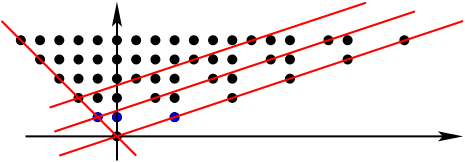
Figure 2. Restriction of the Fourier transform to $y_{1}=0$.

The picture shows in blue the columns of $A$, in black the other elements of $\mathbb{N}A$, in red the quasi-degrees of $N=S_{A}/\partial_{1}\cdot S_{A}$. The roots of $b(\delta_{1}y_{1})$ (which are opposite to the roots of $b(\tilde{\theta}_{1})$) are the intersections of the line $\mathbb{C}\cdot{0\choose 1}$ with the shift of the red lines by $-\beta$.

In this example, each composition factor corresponds to facet and to a component of the quasi-degrees of $N$. One checks that each composition chain must have these four lines as quasi-degrees. Note, however, that composition chains are far from unique and in general such correspondence will not exist.

Remark 2.8.

The $b$-function for $\mathscr{F}^{-1}(M_{A}(\beta))$ along a coordinate hyperplane is generally not reduced, and its degree may be lower than the length of the shortest toric filtration for $N=S_{A}/\partial_{t}\cdot S_{A}$ would suggest. (Not every component of $\beta-\operatorname{qdeg}_{A}(N)$ needs to meet the line $\mathbb{C}\cdot{\mathbf{a}}_{t}$).

Corollary 2.9.

The roots of the $b$-function $b(\delta_{t}y_{t})$ of $\mathscr{F}^{-1}(M_{A}(\beta))$ along $y_{t}=0$ are in the field $\mathbb{Q}(\beta)$.

Consider $\mathscr{F}^{-1}(M_{A}(0))$; then:

1. the roots of the $b$-function $b(\tilde{\theta}_{t})$ are non-negative rationals;

2. if $S_{A}$ is normal, all roots are in the interval $[0,1)$;

3. if the interior ideal of $S_{A}$ is contained in $\partial_{t}\cdot S_{A}$ then zero is the only root.

Proof.

The first claim is a consequence of the intersection property in Theorem 2.5: the defining equations for the quasi-degrees are rational.

Let $N=S_{A}/\partial_{t}S_{A}$. For items 1.-3., we need to study the intersection of $\operatorname{qdeg}_{A}(N)$ with $\mathbb{C}\cdot{\mathbf{a}}_{t}$, since $\beta=0$ and $\delta_{t}y_{t}=-\tilde{\theta}_{t}$. The quasi-degrees of $N$ are covered by hyperplanes of the sort $L_{\alpha}=\varepsilon$ where $L_{\alpha}$ is a rational supporting functional of the facet $F_{\alpha}$. In particular, we can arrange $L_{\alpha}$ to be zero on $F_{\alpha}$, positive on the rest of $A$, and $L_{\alpha}({\mathbf{a}}_{t})=1$. As $\deg_{A}(N)\subseteq\deg_{A}(S_{A})$, $\varepsilon\geq 0$. Hence $\operatorname{Var}(L_{\alpha}-\varepsilon)$ meets $\mathbb{C}\cdot{\mathbf{a}}_{t}$ in the non-negative rational multiple $\varepsilon{\mathbf{a}}_{t}$ of ${\mathbf{a}}_{t}$. If $S_{A}$ is normal, $\deg_{A}(S_{A}/\partial_{A}S_{A})$ is covered by hyperplanes $\operatorname{Var}(L_{\alpha}-\varepsilon)$ that do not meet the cone ${\mathbf{a}}_{t}+\mathbb{R}_{\geq 0}A$. These are precisely the ones for which $\varepsilon<1$.

If $\partial_{t}\cdot S_{A}$ contains the interior ideal then $\deg_{A}(N)$, and hence $\operatorname{qdeg}_{A}(N)$, is inside the supporting hyperplanes of the cone, which meet $\mathbb{C}\cdot{\mathbf{a}}_{t}$ at the origin. ∎

Remark 2.10.

One special case in which case 3 of Corollary 2.9 applies is when $S_{A}$ is Gorenstein and where further $\partial_{t}$ generates the canonical module. The matrix $A=({\mathbf{a}}_{0},\ldots,{\mathbf{a}}_{3})=\begin{pmatrix}1&1&1&1\\ 0&1&3&0\\ 0&0&0&1\end{pmatrix}$, with the interior ideal being generated by $\partial_{1}\partial_{3}$, provides an example that case (3) can occur in a Gorenstein situation without the boundary of $\mathbb{N}A$ being saturated. See [SW09a] for a discussion on Cohen–Maculayness of face rings of Cohen–Macaulay semigroup rings.

3. $b$-functions for the hypergeometric system

3.1. Restriction along a hyperplane

We are here interested in the $b$-function for the hypergeometric module $M_{A}(\beta)$ along the hyperplane $x_{t}=0$. As in the previous section, apart from examples, we actually carry out all computations for $t=0$, in order to have as few variables around as possible. On the other hand, the natural argument for expressing the $b$-function will be $s=x_{0}\partial_{0}$.

Notation 3.1.

With $A=({\mathbf{a}}_{0},\ldots,{\mathbf{a}}_{n})$ and distinguished index $0$, we denote $A^{\prime}:=({\mathbf{a}}_{1},\ldots,{\mathbf{a}}_{n})$. Via $\mathbb{N}A^{\prime}\subseteq\mathbb{N}A$ we consider $S_{A^{\prime}}$ as a subring of $S_{A}$.

For $k\in\mathbb{N}$ let $\overline{J}_{A,0;k}\subseteq S_{A^{\prime}}$ be the vector space spanned by the monomials $\partial^{\mathbf{u}}$ with $u_{0}=0$ (so that $\partial^{\mathbf{u}}\in S_{A^{\prime}}$) that satisfy $\partial_{0}^{k}\cdot\partial^{\mathbf{u}}\in S_{A^{\prime}}$. We denote $J_{A,0;k}\subseteq R_{A^{\prime}}$ the preimage of $\overline{J}_{A,0;k}$ under the natural surjection $R_{A^{\prime}}\twoheadrightarrow S_{A^{\prime}}$. Put $J_{A,0}=\sum_{k\geq 1}J_{A,0;k}$ and $\overline{J}_{A,0}=J_{A,0}/I_{A^{\prime}}\subseteq S_{A^{\prime}}$ .

Each $\overline{J}_{A,0;k}$ is a monomial ideal of $S_{A^{\prime}}$ since $\partial_{0}^{k}(\partial^{\mathbf{v}}\partial^{\mathbf{u}})=\partial^{\mathbf{v}}(\partial_{0}^{k}\partial^{\mathbf{u}})$. Note, however, that $\overline{J}_{A,0;k}$ need not be contained in $\overline{J}_{A,0;k+1}$. If ${\mathbf{a}}_{0}\in\mathbb{R}_{\geq 0}A^{\prime}$ then some power of $\partial_{0}$ is in $S_{A^{\prime}}$ and so $\overline{J}_{A,0}=S_{A^{\prime}}$.

Definition 3.2.

For ${\mathbf{a}}_{0}\in\mathbb{R}^{d}$ outside $\mathbb{R}_{\geq 0}A^{\prime}$, a point ${\mathbf{a}}\in\mathbb{R}_{\geq 0}A^{\prime}$ is ${\mathbf{a}}_{0}$-visible if ${\mathbf{a}}+\lambda\cdot{\mathbf{a}}_{0}$, $0<\lambda\ll 1$ is outside $\mathbb{R}_{\geq 0}A^{\prime}$. (The idea behind the choice of language is that the observer stands at the point of projective space given by the line $\mathbb{R}{\mathbf{a}}_{0}$.)

By abuse of notation, we say that $\partial^{\mathbf{a}}$ is ${\mathbf{a}}_{0}$-visible if ${\mathbf{a}}$ is.

Lemma 3.3.

Assume that ${\mathbf{a}}_{0}$ is not in the cone $\mathbb{R}_{\geq 0}A^{\prime}$. Then the radical of $J_{A,0}$ is generated by the ${\mathbf{a}}_{0}$-invisible elements of $S_{A^{\prime}}$, and in consequence the quasi-degrees of $S_{A^{\prime}}/J_{A,0}$ are a union of shifted face spans where each face is in its entirety visible from ${\mathbf{a}}_{0}$.

Proof.

If $\mathbb{Z}A/\mathbb{Z}A^{\prime}$ has positive rank then all points of $\mathbb{N}A$ are ${\mathbf{a}}_{0}$-visible while $J_{A,0}$ is clearly zero, so that in this case there is nothing to prove. We therefore assume that $\mathbb{Z}A/\mathbb{Z}A^{\prime}$ is finite.

It is immediate that ${\mathbf{a}}$ is ${\mathbf{a}}_{0}$-visible if and only if any positive integer multiple of it is. This implies that no power of an ${\mathbf{a}}_{0}$-visible element $\partial^{\mathbf{a}}$ of $S_{A^{\prime}}$ can be in the radical of $J_{A,0}$ since $\partial^{m\cdot{\mathbf{a}}+k{\mathbf{a}}_{0}}$ can’t have its degree in the cone of $A^{\prime}$.

For the converse, suppose ${\mathbf{a}}$ is not ${\mathbf{a}}_{0}$-visible, so that there are positive integers $p<q$ with ${\mathbf{a}}+(p/q)\cdot{\mathbf{a}}_{0}\in\mathbb{R}_{\geq 0}A^{\prime}$. Then a high power of $\partial^{q\cdot{\mathbf{a}}+p\cdot{\mathbf{a}}_{0}}$ is in $\mathbb{C}[\mathbb{Z}A\cap\mathbb{R}_{\geq 0}A^{\prime}]$ and a suitable power $\partial^{\mathbf{b}}$ of that will be in $\mathbb{C}[\mathbb{Z}A^{\prime}\cap\mathbb{R}_{\geq 0}A^{\prime}]$ because of the finiteness of $\mathbb{Z}A/\mathbb{Z}A^{\prime}$. Now let $\tau$ be the smallest face of $\mathbb{R}_{\geq 0}A^{\prime}$ that contains ${\mathbf{b}}$; this makes ${\mathbf{b}}$ an interior point of $\tau$. Since $\mathbb{C}[\tau\cap\mathbb{Z}A^{\prime}]$ is a finitely generated $\mathbb{C}[\tau\cap\mathbb{N}A^{\prime}]$-module, some power of $\partial^{\mathbf{b}}$ is in $\mathbb{C}[\tau\cap\mathbb{N}A^{\prime}]\subseteq S_{A^{\prime}}$. This shows that some power of $\partial^{q\cdot{\mathbf{a}}}$ times some power of $\partial^{p\cdot{\mathbf{a}}_{0}}$ is in $S_{A^{\prime}}$, establishing the first claim of the lemma.

In every composition chain for $S_{A^{\prime}}/J_{A,0}$, each composition factor is an $S_{A^{\prime}}/\sqrt{J_{A,0}}$-module. Thus the quasi-degrees of $S_{A^{\prime}}/J_{A,0}$ are inside a union of shifted quasi-degrees of $S_{A^{\prime}}/\sqrt{J_{A,0}}$ and hence all ${\mathbf{a}}_{0}$-visible, which implies the second claim. ∎

Our main theorem in this section is:

Theorem 3.4.

The root locus of the $b$-function $b(x_{0}\partial_{0})$ for restriction of $M_{A}(\beta)$ along $x_{0}=0$ is, up to inclusion of non-negative integers, contained in the locus of intersection $(-\operatorname{qdeg}_{A^{\prime}}(S_{A^{\prime}}/\overline{J}_{A,0})+\beta)\cap\mathbb{C}\cdot{\mathbf{a}}_{0}$. The set of integers needed can be taken to be the integers $0,\ldots,k-1$ such that $J_{A,0}=\sum_{1\leq i\leq k}J_{A,0;i}$.

In two extreme cases one can be explicit:

1. if $\dim S_{A}-1=\dim S_{A^{\prime}}$ then the $b$-function is linear with root given by the intersection of $(-\operatorname{qdeg}_{A}(S_{A^{\prime}})+\beta)\cap\mathbb{C}\cdot{\mathbf{a}}_{0}$;

2. if ${\mathbf{a}}_{0}\in\mathbb{R}_{\geq 0}{A^{\prime}}$ then the $b$-function has integer roots in $\{0,1,\ldots,k-1\}$ where $k=\min\{t\in\mathbb{N}\mid 0\not=t\cdot{\mathbf{a}}_{0}\in\mathbb{N}A^{\prime}\}$.

Proof.

We first dispose of the extreme cases. If $\dim S_{A}-1=\dim S_{A^{\prime}}$, then $S_{A}$ is the polynomial ring $S_{A^{\prime}}[\partial_{0}]$ and $A^{\prime}$ is a facet of $A$. By Lemma 1.3 there is ${\mathbf{v}}=(v_{1},\ldots,v_{d})$ such that the Euler operator

$$E-\beta_{E}=\sum v_{i}(E_{i}-\beta_{i})$$

is in $H_{A}(\beta)$ and equals $\theta_{0}-\beta_{E}$. In particular, the $b$-function is $s-\beta_{E}$. On the other hand: $\overline{J}_{A,0}$ is zero in this case, ${\mathbf{v}}=(v_{1},\ldots,v_{d})$ is in the kernel of ${A^{\prime}}^{T}$, and ${\mathbf{a}}_{0}^{T}{\mathbf{v}}=1$. Therefore, the quasi-degrees of $S_{A^{\prime}}/\overline{J}_{A,0}$ form the hyperplane given as the kernel of ${\mathbf{v}}$ and $({\mathbf{v}}^{T}\beta){\mathbf{a}}_{0}=\beta_{E}{\mathbf{a}}_{0}$ is the intersection of $-\operatorname{qdeg}_{A}(S_{A^{\prime}})+\beta$ with $\mathbb{C}{\mathbf{a}}_{0}$.

If ${\mathbf{a}}_{0}\in\mathbb{R}_{\geq 0}A^{\prime}$ then $\mathbb{N}{\mathbf{a}}_{0}$ meets $\mathbb{N}A^{\prime}$ and so $\partial_{0}^{k}=\partial^{\mathbf{u}}$ with ${\mathbf{u}}=(0,u_{1},\ldots,u_{n})\in\mathbb{N}A^{\prime}$. In particular, $J_{A,0}=S_{A^{\prime}}$ in this case. Moreover, $(x_{0}\partial_{0})(x_{0}\partial_{0}-1)\cdots(x_{0}\partial_{0}-k+1)=x_{0}^{k}\partial_{0}^{k}=x_{0}^{k}(\partial_{0}^{k}-\partial^{\mathbf{u}})+x_{0}^{k}\partial^{\mathbf{u}}\in H_{A}(\beta)+V^{1}(D_{A})$ shows the claim made in this case.

Now suppose that $A$ and $A^{\prime}$ have equal rank but ${\mathbf{a}}_{0}\not\in\mathbb{R}_{\geq 0}A^{\prime}$. In that case, $\overline{J}_{A,0}$ is a non-trivial ideal of $S_{A^{\prime}}$. We shall use a toric filtration

$$(N)\quad:\quad 0=N_{0}\subsetneq N_{1}\subsetneq\ldots\subsetneq N_{t}=S_{A^{\prime}}/\overline{J}_{A,0}$$

and let $J_{\alpha}\supseteq J_{A,0}$ be the $R_{A^{\prime}}$-ideal such that $N_{\alpha}=J_{\alpha}/J_{A,0}$. We will view $J_{\alpha}$ as subset of $D_{A^{\prime}}$ or even $D_{A}$. In analogy to the previous case, for any $\partial^{\mathbf{u}}$ in $J_{A,0;k}$ the $b$-function along $x_{0}$ of the coset of $\partial^{\mathbf{u}}$ in $M_{A}(\beta)$ divides $s(s-1)\cdots(s-k+1)$. Indeed, $\partial^{\mathbf{u}}\in J_{A,0;k}$ implies that $\partial_{0}^{k}\partial^{\mathbf{u}}-\partial^{\mathbf{v}}\in I_{A}$ for some ${\mathbf{v}}$ with $v_{0}=0$, and so $x_{0}^{k}\partial_{0}^{k}\partial^{\mathbf{u}}\in H_{A}(\beta)+V^{1}(D_{A})$. In particular, the root set of the $b$-function of the coset of $\partial^{\mathbf{u}}$ in $M_{A^{\prime}}(\beta)$ is inside the set of integers described in the statement of the theorem.

For each composition factor $\overline{N}_{\alpha}=N_{\alpha}/N_{\alpha-1}$ choose now a facet $\tau_{\alpha}$ of $A^{\prime}$ and an element $\partial^{{\mathbf{u}}_{\alpha}}$ of $S_{A^{\prime}}$ ${\mathbf{u}}_{\alpha}\in\{0\}\times\mathbb{N}^{n}$ such that $N_{\alpha}$ is a quotient of $S_{A^{\prime}}\cdot\partial^{{\mathbf{u}}_{\alpha}}$ and such that the annihilator of $\partial^{{\mathbf{u}}_{\alpha}}$ in $\overline{N}_{\alpha}$ contains the toric ideal $I_{A^{\prime}}^{\tau_{\alpha}}$. Then $\operatorname{qdeg}_{A^{\prime}}(\overline{N}_{\alpha})$ is contained in $A^{\prime}\cdot{\mathbf{u}}_{\alpha}+\operatorname{qdeg}_{A^{\prime}}(S_{\tau_{\alpha}})$.

Since ${\mathbf{a}}_{0}$ is not in $\mathbb{R}_{\geq 0}A^{\prime}$, Lemma 3.3 shows that the facet $\tau_{\alpha}$ can be chosen such that ${\mathbf{a}}_{0}\not\in\mathbb{Q}\cdot\tau_{\alpha}$. Indeed, if an entire face of $\mathbb{R}_{\geq 0}A^{\prime}$ is visible from ${\mathbf{a}}_{0}$ then it sits in at least one facet whose span does not contain ${\mathbf{a}}_{0}$. By Lemma 1.3 there is an element $E_{\alpha}$ of the Euler space of $A$ that does not involve any element of $\tau_{\alpha}$, but which has coefficient $1$ for $\theta_{0}$. Notation 1.2 then associates a degree function $\deg_{E_{\alpha}}(-)$ to $\alpha$.

As $\partial_{j}\cdot\partial^{{\mathbf{u}}_{\alpha}}\in N_{\alpha-1}$ for $j\not\in\tau_{\alpha}$ it follows that the difference of $(E_{\alpha}-\beta_{\alpha})\cdot\partial^{{\mathbf{u}}_{\alpha}}$ and $(\theta_{0}-\beta_{\alpha})\cdot\partial^{{\mathbf{u}}_{\alpha}}$ is inside $(V^{0}D_{A})N_{\alpha-1}$. Since $E_{\alpha}-\beta_{\alpha}$ is in $H_{A}(\beta)$, so is $\partial^{{\mathbf{u}}_{\alpha}}(E_{\alpha}-\beta_{\alpha})=(E_{\alpha}-\beta_{\alpha}+\deg_{E_{\alpha}}(\partial^{{\mathbf{u}}_{\alpha}}))\partial^{{\mathbf{u}}_{\alpha}}$. Therefore, $(\theta_{0}-\beta_{\alpha}+\deg_{E_{\alpha}}(\partial^{{\mathbf{u}}_{\alpha}}))\partial^{{\mathbf{u}}_{\alpha}}$ is in $H_{A}(\beta)+(V^{0}D_{A})N_{\alpha-1}$. Then, in parallel to how Lemma 2.4 was used in the proof of Theorem 2.5, the product

$$\prod_{\alpha}(\theta_{0}-\beta_{\alpha}+\deg_{E_{\alpha}}(\partial^{{\mathbf{u}}_{\alpha}}))$$

multiplies $1\in D_{A}$ into $H_{A}(\beta)+(V^{0}D_{A})J_{A,0}+(V^{1}D_{A})$. Multiplying by $x_{0}^{k}\partial_{0}^{k}$ for suitable $k$ one obtains the desired bound for the $b$-function as in the second paragraph of the proof.

It follows as in Theorem 2.5 (with the modification that we have here $\theta_{0}$ rather than $\mathscr{F}^{-1}(\theta_{0})$, which affects signs) that the intersection of the roots of all such bounds is the intersection of $(-\operatorname{qdeg}_{A^{\prime}}(S_{A^{\prime}}/\overline{J}_{A,0})+\beta)$ with the line $\mathbb{C}\cdot{\mathbf{a}}_{0}$. ∎

Example 3.5.

With $A=({\mathbf{a}}_{0},{\mathbf{a}}_{1},{\mathbf{a}}_{2})=\begin{pmatrix}-1&0&3\\ 1&1&1\end{pmatrix}$, consider the $b$-function along $x_{1}$ of the $A$-hypergeometric system. The ideal $J_{A,1}$ is generated by $1\in S_{A^{\prime}}=\mathbb{C}[\mathbb{N}({\mathbf{a}}_{0},{\mathbf{a}}_{2})]$ since $\partial_{1}^{4}$ is in $S_{A^{\prime}}$. The set of necessary integer roots is then $\{0,1,2,3\}$. No other roots are needed since $S_{A}/J_{A,1}$ is zero, irrespective of $\beta$.

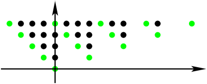
Figure 3. The elements of $S_{A}\smallsetminus S_{A^{\prime}}$ (black) and $S_{A^{\prime}}$ (green) for restriction to $x_{1}$

Restriction to $(x_{2}=0)$ behaves differently. As $S_{A^{\prime}}=\mathbb{C}[\mathbb{N}({\mathbf{a}}_{0},{\mathbf{a}}_{1})]$ now, $J_{A,2}=J_{A,2;1}$ is generated by $\partial_{0}^{3}$, and the quasi-degrees of $S_{A^{\prime}}/J_{A,2}$ are the lines $\mathbb{C}\cdot(0,1)+(i,0)$ with $i=0,-1,-2$.

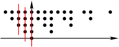
Figure 4. The quasi-degrees of $S_{A}/J_{A,2}$ form three parallel lines.

The intersection of the negative of these three lines, shifted by $\beta$, with the line $\mathbb{C}\cdot{\mathbf{a}}_{2}$ is ${\mathbf{a}}_{2}\cdot\{(i+\beta_{1})/3\}_{i=0,1,2}$. So the $b$-function has (at worst) roots $\{0,\beta_{1},\beta_{1}+1,\beta_{1}+2\}/3$.

Remark 3.6.

We believe that both bounds in Theorems 2.5 (as is) and 3.4 (up to integers) are sharp.

3.2. Restriction to a generic point

We suppose here that $A$ is homogeneous; in other words, the Euler space contains a homothety. Let $p=(p_{0},\ldots,p_{n})$ be a point of $\mathbb{C}^{n+1}$. We wish to estimate here the $b$-function for restriction of $M_{A}(\beta)$ to the point $-p$ if $p$ is generic. As a holonomic module is a connection near any generic point, this restriction yields a vector space isomorphic to the space of solutions to $H_{A}(\beta)$ near $-p$, see [SST00, Sec. 5.2].

Definition 3.7.

Let $\theta_{p}=(x_{0}+p_{0})\partial_{0}+\ldots+(x_{n}+p_{n})\partial_{n}$ and write $\theta$ for $\theta_{p}$ if $p=0$. The $b$-function for restriction of a principal $D$-module $M=D/I$ to the point $x+p=0$ is the minimal polynomial $b_{p}(s)$ such that $b_{p}(\theta_{p})\in I+(V^{1}_{p}D)$ where $V^{k}_{p}D$ is the Kashiwara–Malgrange $V$-filtration along $\operatorname{Var}(x+p)$:

$$V^{k}_{p}D=\mathbb{C}\cdot\{(x+p)^{\mathbf{u}}\partial^{\mathbf{v}}\quad\mid\quad|{\mathbf{u}}|-|{\mathbf{v}}|\geq k\}.$$

Remark 3.8.

1. For any pair of manifolds $Y\subseteq X$ and given a $D$-module $M$ on $X$ one can define a $b$-function of restriction for the section $m\in M$ along $Y$ by a formula generalizing both Definition 0.1 and Definition 3.7. Kashiwara proved their existence for holonomic $M$.

2. The roots of this $b$-function here relate to restriction of solution sheaves as follows. Near a generic point $x+p=0$, a $D$-module $M$ is a connection whose solution space has a basis consisting of a certain number of holomorphic functions. The germs of these functions form a vector space that can be identified with the dual of the $0$-th homology group of $(D/(x+p)D)\otimes^{L}_{D}M$. Filtering this complex by $V^{\bullet}_{p}D$, $b_{p}(k)$ annihilates the $k$-th graded part of its homology, compare [Oak97, OT01, Wal00]. In particular, $b_{p}(s)$ carries information on the starting terms of the solution sheaf of $M$ near $x+p=0$.

The purpose of this section is to bound $b_{p}(s)$ for $I=H_{A}(\beta)$ and generic $p$ with the following strategy. We first show that a polynomial $b(s)$ is a multiple of $b_{p}(s)$ if $b(\theta)$ is in $D_{A}(I_{A},A\cdot{\mathscr{E}}\cdot\partial)$ where

$${\mathscr{E}}=\begin{pmatrix}p_{0}&0&\cdots&0\\ 0&p_{1}&&\vdots\\ \vdots&&\ddots&0\\ 0&\cdots&0&p_{n}\end{pmatrix},$$

provided that $p$ is component-wise nonzero. The generators of $D_{A}(I_{A},A\cdot{\mathscr{E}}\cdot\partial)$ are independent of $x$ and we next observe that the radical of $R_{A}(I_{A},A\cdot{\mathscr{E}}\cdot\partial)$ is $R_{A}\cdot\partial$, provided that $p$ is generic. Thus, $b_{p}(s)$ will be a factor of any polynomial that annihilates the finite length module $R_{A}/(I_{A},A\cdot{\mathscr{E}}\cdot\partial)$ as long as $p$ is generic. We exhibit a particular such polynomial with all roots integral. In the case of a normal semigroup ring, we show that the (necessarily integral) roots of $b_{p}(s)$ are in the interval $[0,d-1]$.

We begin with pointing out that $b(\theta_{p})\in I+(V^{1}_{p}D)$ is equivalent to $b(\theta)\in I_{p}+(V^{1}_{0}D)$ where $I_{p}$ is the image of $I$ under the morphism induced by $x\mapsto x-p$, $\partial\mapsto\partial$ and $(V^{k}_{0}D)$ is the Kashiwara–Malgrange filtration along the origin. Among the generators of $I=H_{A}(\beta)$, only the Euler operators depend on $x$ while $(I_{A})_{p}=I_{A}$ for any $p$; one has $(E_{i}-\beta_{i})_{p}=\sum a_{i,j}(x_{j}-p_{j})\partial_{j}-\beta_{i}=E_{i}-\beta_{i}-\sum a_{i,j}p_{j}\partial_{j}$. We hence seek a relation $b(\theta)\in D_{A}\cdot(I_{A},E-\beta-A\cdot{\mathscr{E}}\cdot\partial)+(V^{1}_{0}D_{A})$ with ${\mathscr{E}}$ as above.

Generally, a statement $b(\theta)\in I+(V^{1}_{0}D_{A})$ is equivalent to $b(\theta)$ being in the degree zero part $\operatorname{gr}^{0}_{V_{0}}(I)$ of the associated graded object. Note that $\operatorname{gr}_{V_{0}}(D_{A})$ is a Weyl algebra again (although of course the symbol map $D_{A}\longrightarrow\operatorname{gr}_{V_{0}}(D_{A})$ is not an isomorphism). Abusing notation, we denote $x$ and $\partial$ also the symbols in $\operatorname{gr}_{V_{0}}(D_{A})$ of the respective elements of $D_{A}$. By the previous paragraph then, the graded ideal $\operatorname{gr}_{V_{0}}(H_{A}(\beta)_{p})$ contains the elements that generate $I_{A}$ (since $I_{A}$ is homogeneous!), as well as the elements $A\cdot{\mathscr{E}}\cdot\partial$ which arise as the $V_{0}$-symbols of $E_{p}-\beta$.

We need the following folklore result ) for which we know no explicit reference.

Claim.

The $R_{A}$-ideal generated by $I_{A}$ and $A\cdot{\mathscr{E}}\cdot\partial$ has, for generic ${\mathscr{E}}$, radical $R_{A}\cdot\partial$.

A sequence of $d$ generic linear forms is of course a system of parameters on $S_{A}$; the issue is to show that linear forms of the type $A\cdot{\mathscr{E}}\cdot\partial$ are sufficiently generic.

Proof.

As $I_{A}$ and $A\cdot{\mathscr{E}}\cdot\partial$ are standard graded, $\operatorname{Var}(I_{A},A\cdot{\mathscr{E}}\cdot\partial)$ is a conical variety. It thus suffices to show that the ideal $\operatorname{Var}(I_{A},A\cdot{\mathscr{E}}\cdot\partial)$ is of height $n+1$.

The ideal $R_{A}[x](I_{A},A\cdot\theta)$ in the polynomial ring $R_{A}[x]$ defines in the cotangent bundle $\operatorname{Spec}(R_{A}[x])$ of $\mathbb{C}^{n+1}$ the union of the conormals to each torus orbit since the Euler fields are tangent to the torus and span a space of the correct dimension in each orbit point. Suppose the claim is false, so that there is a nonzero point $y\in\operatorname{Var}(I_{A})$ such that (the generically chosen vector) $p$ is a conormal vector to the orbit of $y$. If $y$ is in a torus orbit $O_{\tau}$ associated to a proper face $\tau$ of $A$ then its coordinates corresponding to $A\smallsetminus\tau$ are zero and we can reduce the question to the case where $A=\tau$. It is hence enough to show that there is $p\in\mathbb{C}^{n+1}$ such that $p$ is not a conormal vector to any smooth point of $\operatorname{Var}(I_{A})$.

Let $X\subseteq\mathbb{C}^{n+1}$ be any reduced affine variety and denote $X_{0}$ its smooth locus. We define a set $C(X)$ inside $\mathbb{C}^{n+1}$ by setting

$$[\eta\in C(X)]\iff[\exists y\in X_{0},\quad\eta\in(T^{*}_{X_{0}}(\mathbb{C}^{n+1}))_{y}]$$

where $(T^{*}_{X_{0}}(\mathbb{C}^{n+1}))_{y}$ is the fiber of the conormal bundle at $y$ of the pair $X_{0}\subseteq\mathbb{C}^{n+1}$. This is a constructible, analytically parameterized union of a $\dim(X)$-dimensional family of vector spaces of dimension $n+1-\dim(X)$, which hence might fill $\mathbb{C}^{n+1}$.

Now suppose that $X$ is a conical variety; then the conormals of $y$ and $\lambda y$ agree for all $\lambda\in\mathbb{C}^{*}$. In particular,

$$C(X)=\bigcup_{\overline{y}\in\operatorname{Proj}(X)}(T^{*}_{X_{0}}(\mathbb{C}^{n+1}))_{y}$$

where $\operatorname{Proj}(X)$ is the associated projective variety. But this is now an analytically parameterized union of a $(\dim(X)-1)$-dimensional family of vector spaces of dimension $n+1-\dim(X)$. It follows that most elements of $\mathbb{C}^{n+1}$ are outside $C(X)$ in this case, and the claim follows. ∎

It follows from the Claim that $\operatorname{gr}_{V_{0}}(H_{A}(\beta)_{p})$ contains all monomials in $\partial$ of a certain degree $k$ that depends on $A$. Let $E=\theta_{0}+\ldots+\theta_{n}$; by hypothesis $E-\beta_{E}\in H_{A}(\beta)$.

Lemma 3.9.

Denote $\partial_{A}^{k}$ the set of all monomials of degree $k$ in $\partial_{0},\ldots,\partial_{n}$, and $D_{A}\cdot\partial_{A}^{k}$ the left $D_{A}$-ideal generated by $\partial_{A}^{k}$. Then in $D_{A}/D_{A}\cdot\partial_{A}^{k}$, the identity $E(E-1)\cdots(E-k+1)\cong 0$ holds.

Proof.

This is clear if $k=1$. In general, by induction,

$$E(E-1)\cdots(E-k+1)\in D_{A}\cdot\partial_{A}^{k-1}\cdot(E-k+1)=D_{A}\cdot E\cdot\partial_{A}^{k-1}\subseteq D_{A}\cdot\partial_{A}^{k}.$$

∎

Remark 3.10.

The homogeneity of $X$ is necessary in the Claim, since otherwise $C(X)$ does not need to be contained in a hypersurface. Consider, for example, $A=(2,1)$ in which case the union of all tangent lines (nearly) fills the plane, and where the zero locus of $I_{A}$ and $A\cdot{\mathscr{E}}\cdot\partial$ contains always at least two points.

The lemma implies that $\operatorname{gr}_{V_{0}}^{0}(H_{A}(\beta)_{p})$ contains $E(E-1)\cdots(E-k+1)$ if $p$ is generic. In other words, the $b$-function for restriction of $M_{A}(\beta)$ to a generic point divides $s(s-1)\cdots(s-k+1)$.

In some cases one can be more explicit about $k-1$, the top degree in which $R_{A}/R_{A}(I_{A},A\cdot{\mathscr{E}}\cdot\partial)$ is nonzero. Suppose $S_{A}$ is a Cohen–Macaulay ring, then systems of parameters are regular sequences. In particular, the Hilbert series of $Q_{A}:=R_{A}/R_{A}(I_{A},A\cdot{\mathscr{E}}\cdot\partial)$ is that of $S_{A}$ multiplied by $(1-t)^{d}$. Suppose in addition, that $S_{A}$ is normal. Since we already assume that $S_{A}$ is standard graded, let $P$ be the polytope that forms the convex hull of the columns of $A$. The Hilbert series of $S_{A}$ is then of the form $\sum_{m=0}^{\infty}p_{m}\cdot t^{m}$ where $p_{m}$ is the number of lattice points in the dilated polytope $m\cdot P$. This number of lattice points is counted by the Erhart polynomial $E_{P}(m)$ of $P$, a polynomial of degree $d-1=\dim(P)$. If one writes the Hilbert series of $S_{A}$ in standard form $Q(t)/(1-t)^{d}$ then the Hilbert series of $Q_{A}$ is just the polynomial $Q(t)$. In particular, the highest degree of a non-vanishing element of $Q_{A}$ is the degree of $Q(t)$.

In order to determine $\deg(Q(t))$ let $E_{P}(m)=e_{d-1}m^{d-1}+\ldots+e_{0}$. Now in

$$\sum_{m=0}^{\infty}E_{P}(m)t^{m}=\sum_{i=0}^{d-1}\left(e_{i}\cdot\sum_{m=0}^{\infty}m^{i}\cdot t^{m}\right),$$

each term $\sum_{m=0}^{\infty}m^{i}\cdot t^{m}$, for $m>0$, is a polylogarithm $\operatorname{Li}_{-i}(t)$ given by $(t\frac{{\mathrm{d}}}{{\mathrm{d}}t})^{n}(\frac{t}{1-t})$. A simple calculation shows that $\operatorname{Li}_{-i}(t)$ is the quotient of a polynomial of degree $i-1$ by $(1-t)^{i}$. Hence the sum in the display is the quotient of a polynomial of degree at most $d-1$ by $(1-t)^{d}$. The degree is truly $d-1$ as one can check from the differential expression for $\operatorname{Li}_{-i}(t)$ above.

Therefore, the Hilbert series $Q(t)$ of $Q_{A}$ is a polynomial of degree $d-1$. We have proved

Theorem 3.11.

Let $S_{A}$ be standard graded. The $b$-function for restriction of $M_{A}(\beta)$ to a generic point $x+p=0$ divides $s(s-1)\cdots(s-k+1)$ where $k$ denotes the highest degree in which the quotient $S_{A}/S_{A}\cdot(A\cdot{\mathscr{E}}\cdot\partial)$ is nonzero. If, in addition, $S_{A}$ is normal then one may take $k=d$.∎

References

- [FFW11] María-Cruz Fernández-Fernández and Uli Walther. Restriction of hypergeometric -modules with respect to coordinate subspaces. Proc. Amer. Math. Soc., 139(9):3175–3180, 2011.
- [Gel86] I. M. Gel′fand. General theory of hypergeometric functions. Dokl. Akad. Nauk SSSR, 288(1):14–18, 1986.
- [Hot98] Ryoshi Hotta. Equivariant -modules. arXiv:math/9805021, pages 1–30, 1998.
- [Kas77] Masaki Kashiwara. -functions and holonomic systems. Rationality of roots of -functions. Invent. Math., 38(1):33–53, 1976/77.
- [MM04] Philippe Maisonobe and Zoghman Mebkhout. Le théorème de comparaison pour les cycles évanescents. In Éléments de la théorie des systèmes différentiels géométriques, volume 8 of Sémin. Congr., pages 311–389. Soc. Math. France, Paris, 2004.
- [MMW05] Laura Felicia Matusevich, Ezra Miller, and Uli Walther. Homological methods for hypergeometric families. J. Amer. Math. Soc., 18(4):919–941 (electronic), 2005.
- [Oak97] Toshinori Oaku. Algorithms for -functions, restrictions, and algebraic local cohomology groups of -modules. Adv. in Appl. Math., 19(1):61–105, 1997.
- [OT01] Toshinori Oaku and Nobuki Takayama. Algorithms for -modules—restriction, tensor product, localization, and local cohomology groups. J. Pure Appl. Algebra, 156(2-3):267–308, 2001.
- [Rei14] Thomas Reichelt. Laurent polynomials, GKZ-hypergeometric systems and mixed Hodge modules. Compos. Math., 150(6):911–941, 2014.
- [RS15] Thomas Reichelt and Christian Sevenheck. Hypergeometric Hodge modules. arXiv:1503.01004, pages 1–48, 2015.
- [Sai88] Morihiko Saito. Modules de Hodge polarisables. Publ. Res. Inst. Math. Sci., 24(6):849–995 (1989), 1988.
- [SST00] Mutsumi Saito, Bernd Sturmfels, and Nobuki Takayama. Gröbner deformations of hypergeometric differential equations, volume 6 of Algorithms and Computation in Mathematics. Springer-Verlag, Berlin, 2000.
- [SW08] Mathias Schulze and Uli Walther. Irregularity of hypergeometric systems via slopes along coordinate subspaces. Duke Math. J., 142(3):465–509, 2008.
- [SW09a] Mathias Schulze and Uli Walther. Cohen-Macaulayness and computation of Newton graded toric rings. J. Pure Appl. Algebra, 213(8):1522–1535, 2009.
- [SW09b] Mathias Schulze and Uli Walther. Hypergeometric D-modules and twisted Gauß-Manin systems. J. Algebra, 322(9):3392–3409, 2009.
- [Wal00] Uli Walther. Algorithmic computation of de Rham cohomology of complements of complex affine varieties. J. Symbolic Comput., 29(4-5):795–839, 2000. Symbolic computation in algebra, analysis, and geometry (Berkeley, CA, 1998).