Complex bifurcations in Bénard-Marangoni convection

Abstract

We study the dynamics of a system defined by the Navier-Stokes equations for a non-compressible fluid with Marangoni boundary conditions in the two dimensional case. We show that more complicated bifurcations can appear in this system for a certain nonlinear temperature profile as compared to bifurcations in the classical Rayleigh-Bénard and Bénard-Marangoni systems with simple linear vertical temperature profiles. In terms of the Bénard-Marangoni convection, the obtained mathematical results lead to our understanding of complex spatial patterns at a free liquid surface, which can be induced by a complicated profile of temperature or a chemical concentration at that surface. In addition, we discuss some possible applications of the results to turbulence theory and climate science.

Keywords: Bénard-Marangoni convection, Navier-Stokes equations, bifurcation, surface tension, temperature

1 Introduction

The study of bifurcations in fluid and climate systems has attracted the attention of many researchers in connection with climate tipping point problems (see [1] for an overview) and turbulence [2, 3]. In particular, in [3] a hypothesis is pioneered that fluid turbulence can appear as a result of bifurcations from a simple dynamics to a chaotic dynamics.

In this paper, we show, in an analytical way, that some spatially inhomogeneous fluid systems are capable of exhibiting a large spectrum of complicated bifurcations. At a bifurcation point, we observe a transition from a steady state attractor to chaotic dynamics and complex spatio-temporal patterns, which are quasiperiodical in space and chaotic in time. These patterns describe coherent turbulent structures (see Fig. 1).

We have an explicit analytic description of turbulent onset. In these turbulent patterns, the chaotic attractor dimension and dynamics are controllable by space inhomogeneities, and although that control is complicated, it is quite constructive. The dynamics at the bifurcation point is defined by so-called normal forms. We show that all kinds of structurally stable dynamics can appear as normal forms as we vary system space inhomogeneities.

To explain the physical ideas behind complicated mathematics and to understand this new bifurcation mechanism, let us recall the classical results on Rayleigh-Bénard and Bénard-Marangoni bifurcations. They show that, for simple linear temperature profiles $U(y)$, where $y$ is the vertical coordinate, the bifurcation is a result of a single mode instability. This mode is periodic in $x$ with period $T=2\pi/k$, where $k$ is a wave vector. The instability arises if, for a given $k$, the real part $r_{k}(b)=Re\lambda_{k}(b)$ of the eigenvalue $\lambda_{k}$ corresponding to this mode goes through $0$ as a bifurcation parameter $b$ passes through a critical point $b=b_{c}$. For $b<b_{c}$ we determine that the trivial zero solution of fluid equations is stable, and for $b$ close to $b_{c}$ we find stable solutions describing periodical patterns. The amplitudes of these patterns can be found by a system of differential equations [4, 5, 6], which can be considered as a ”normal form” of the system at the bifurcation point. That normal form determines the dynamics of slow modes in the system. The dynamics of the fast modes is captured, for large times, by slow modes [7]. For many bifurcations the normal form is defined by a system with quadratic nonlinearities, since for small amplitudes the main nonlinear contributions are quadratic [7]. In particular, for the Marangoni case, an analysis of this system shows that the system bifurcates into two steady state solutions, which are local attractors [6].

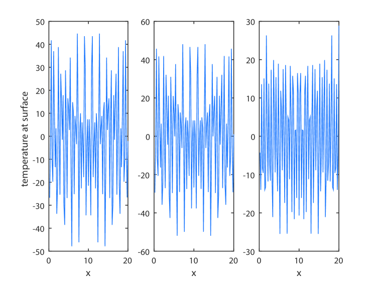
Figure 1: Temperature patterns at the surface $y=0$ as functions of $x$ for times $t=1000,2000$ and $t=3000$. Here slow dynamics at the bifurcation point is defined by $3$ slow modes. Dynamics of these modes is defined by the Lorenz system. The wave numbers of these modes are $k_{1}=1,k_{2}=2.1$ and $k_{3}=3.3$. For generic $k_{i}$ such patterns are quasiperiodic and essentially one-dimensional since they are localized at the top boundary $y=0$ (rather then the space periodic patterns found for the Rayleigh-Bénard problem [5] and for the Lorenz model)

We use a new scheme to obtain much more complicated bifurcations and attractors. This scheme is illustrated by Fig. 2.

1. First, the number of slow modes $n$ is controllable by the space inhomogeneity.

2. These slow modes are associated with eigenfunctions $\psi_{i}$ of a linear operator that describe linearization of system. The functions $\psi_{i}$ are defined by different wave vectors $k_{i}$, $i=1,...,n$. Moreover, the values of $k_{i}$ are completely controlled by the system space inhomogeneity. We can get any sets of $k_{i}$.

3. Lastly, the quadratic normal form is also completely controllable by the space inhomogeneities. We can obtain any quadratic system by a variation of system space inhomogeneities.

The key point (iii) allows us to exhibit the existence of chaotic dynamics. This is found in [8], where it is shown that all kinds of structurally stable dynamics can be generated by quadratic systems. Thus, all structurally stable dynamics can appear as a result of bifurcations. Such bifurcations can be named superbifurcations.

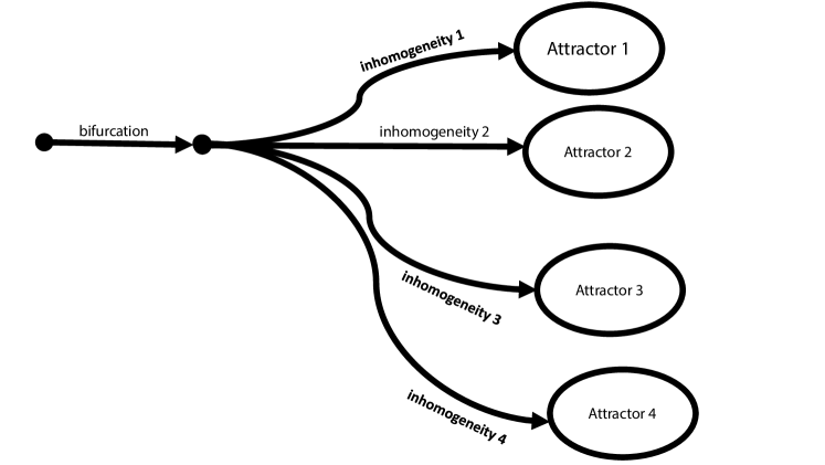
Figure 2: Control of bifurcations by space inhomogeneities in spatially extended systems. This scheme works for reaction-diffusion systems [9] and we propose that it may work for climate systems.

Note that space inhomogeneities consist of two terms. The first term is basic and depends on the vertical coordinate $y$ only. An appropriate choice of this term leads to realization of points (i) and (ii). The second term is small with respect to the first but depends on both vertical and horizontal coordinates. Variations of this term allow us to control the normal forms. The fact that the normal forms sharply depend on small inhomogeneities may be interesting for climate theory. Indeed, we need points (i) and (ii) to create a number of slow modes whereas a possibility of complex interactions between these modes follows from (iii). A typical climate system involves a number of slow modes (see [5, 10]). We can expect that in such systems small space inhomogeneities can lead to complex bifurcations. This property may be important for tipping point theory, which, up to now, considered relatively simple bifurcations in simplified models (see [10] for an overview).

In this paper, we consider local bifurcations only where the dynamics at the bifurcation point is weakly nonlinear. Although we show the existence of complex phenomena and the appearance of chaotic attractors of all dimensions, fully nonlinear systems can also exhibit non-local bifurcations that are harder to describe by the analytical methods of this paper. However, one can expect that if even local bifurcations lead to all kinds of chaos of any dimension, then the same fact also holds for non-local ones.

The solution methodology can be described as follows. According to standard bifurcation ideas, at the bifurcation point the system of solutions can be represented as sums of contributions of slow modes. Each contribution is defined by the corresponding magnitude $X_{k}(t)$, which is a slow function of time $t$. The spatial patterns corresponding to our solutions are complex, they are quasiperiodic in $x$ (horizontal axis) and localized at the surface. Dynamics of the magnitude $X_{k}$ may be time periodic or even chaotic. We thus have complex coherent spatio-temporal patterns quasiperiodic in space, localized at the surface, and evolving in time in a complex manner (see Fig. 1). Moreover, we can control the pattern structure and dynamics. The mathematical realization of that control is based on a vector-field realization approach (the RVF method, see section 8.2 in the Appendix and [8, 11, 12, 13]). This method was successfully applied to many dissipative systems of chemical kinetics and neural network theory. Here, we first use the RVF for fluid dynamics.

We believe that these ideas can be used for many systems, for example, for climate systems. Indeed, climate systems include fast and slow variables and involves spatial inhomogeneities [14]. One can expect that the mechanism of generation of complex large time behaviour, outlined above, works in these systems.

In this paper, for simplicity, we study a toy model having physical applicability. We consider the Navier-Stokes (NS) equations for a non-compressible fluid with the Marangoni boundary conditions in the two dimensional case. These equations describe hydrodynamical systems involving convection, heat transfer and capillarity, and exhibit interesting pattern formation effects [15] (for example, Bénard cells studied in many works [4, 6, 16] and references therein). As indicated in Fig.3, the Marangoni flows are driven by surface tension gradients. In general, surface tension depends on both the temperature and chemical composition at an interface. Therefore, these flows may be generated by gradients in either temperature or chemical concentrations.

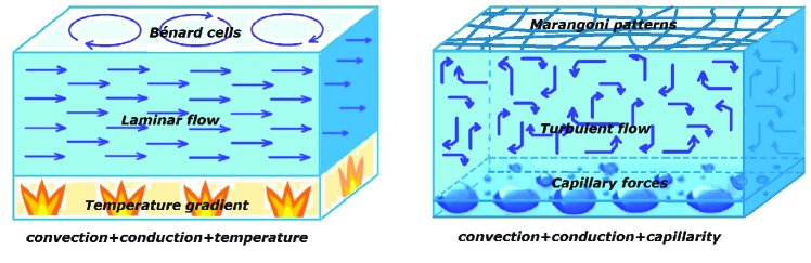
Figure 3: On the left: Bénard convection cells, which are formed by temperature gradients; on the right: the Marangoni patterns are driven by surface tension gradients.

In physical and chemical systems the Marangoni effects are well-known and this may have potential applications for geosystems. For example, shallow permafrost lakes in tundra emit a huge amount of methane that affects the atmospheric dynamics and atmospheric thermodynamics. Apparently, the ”surface tension” in the system of permafrost lake patterns on the tundra’s surface will define methane emission regimes [17]. However, the Marangoni effects also can influence large ecosystems, for example oceanic ones, if there are salinity gradients [18]. In addition, the surface tension of green algal which bloom on the surface of big lakes in Southeast Asia (and fully cover the lake surface), changes the internal physical and chemical properties of these lakes [19]. Finally, the surface tension at the air-water-sedimentary rock interface of geothermal hot springs defines the dynamics of water flows [20].

An interesting situation, where these effects are essential, arises when there exist surfactants on the water surface. The capillary forces are also important for a correct description of air bubble motion. In this paper, we consider thermocapillary Marangoni effects; however, the same analysis is valid when these effects are induced by convection, capillary forces and diffusion, for example, by salinity gradients.

Our plan to find complicated bifurcations is as follows. Let us first fix the fluid viscosity and all other parameters except the Marangoni number $b$, which serves as a bifurcation parameter. This Marangoni parameter $b$ is the ratio of the destabilizing surface tension gradient to the forces generated by thermal and viscous diffusion [6]. We consider general nonlinear profiles $U(y)$ depending on the vertical coordinate only. First, we remove nonlinear terms and consider the corresponding linearized problem. As above, the eigenfunctions of this problem are periodic in $x$ with the period $T=2\pi/k$, where $k$ is a wave vector. For example, the fluid stream function $\psi(x,y)$ induced by these modes has the form $\psi_{k}=\Psi_{k}(y,\lambda)\cos(kx)$. For large Prandtl numbers we obtain an asymptotic equation for $\lambda$. The physical meaning of this equation is transparent; for each wave vector the eigenvalue $\lambda(k)$ is defined by an interaction between the corresponding mode $\psi_{k}$ and the inhomogeneity $U(y)$. Our goal is to find profiles $U(y)$ for which the stability loss occurs simultaneously for many $k$, i.e., we have that the real parts $r_{k}(b)=Re\lambda_{k}(b)$ pass through $0$ for all $k=k_{1},k_{2},...,k_{N}$ as $b$ goes through $b_{c}$.

The key idea in finding such profiles is as follows. First we find a profile $V(y)$ such that the spectrum $\lambda(k)$ is independent of $k$ within a large interval of values $k$. For example, we take $V$ as a step function, where a step localized at the surface $y=0$, for example, at $y=z_{0}<<h$, where $h$ is the depth of fluid layer. There are other possible kinds of $V$, for example, exponential profiles. Then the interaction between the fluid and the inhomogeneity $U$ weakly depends on the wave vector $k$. Therefore, the stability loss will occur simultaneously for a number of $k$ (see comment at the formulation of Theorem 4.2). Indeed, numerical simulations and analytic arguments (see Sect. 4 and Fig. 4) show that, for an appropriate $b=b_{c}$, the quantities $r_{k}(b)$ changes their sign at $b=b_{c}$ for a set of $k$. Then we take the profile $U$ as a weak perturbation of $V$. This trick aims to attain two key goals:

a) we obtain the stability loss at prescribed $k_{1},k_{2},...,k_{N}$ for each $N$ and these $k_{j}$ define wave vectors of slow modes; b) we shift all the other eigenvalues corresponding to $k\neq k_{j}$ towards the left half-plane $Re\lambda<0$ and therefore the corresponding modes are fast.

Furthermore, we take into account nonlinear terms. At the bifurcation point, by standard methods of invariant manifold theory [12, 13, 21], we derive a system of differential equations with quadratic nonlinearities for mode magnitudes $X_{j}(t)$, $j=1,...,N$, that is reminiscent of the Lorenz system. Previous results [8, 11] show that the corresponding dynamical system can have periodic or chaotic trajectories.

Note that the main technical mathematical difficulties are connected with points (i) and (ii). The application the method of realization of vector fields (see Appencix and [9, 12, 13]) of (iii) is standard.

These mathematical results admit a simple physical interpretation. They describe a complex spatial pattern at a free water surface, which can be induced by a complicated profile of temperature or a chemical concentration at that surface. Note that such profiles of salinity concentrations arise in real fluid systems (see [18]). To obtain the complicated profile, we use spatially distributed inhomogeneous sources; however, an analytical proof of the existence of even more complex solutions determined by a non-trivial temperature profile is obtained in paper [22] for the case of a planar free Bénard-Marangoni convection.

This paper is organized as follows. In the next section we formulate the Marangoni problem. In Section 3 we introduce the main linear operator associated with the problem. In Section 4 we investigate the spectrum of this operator, and we state the main new conclusion of the paper and its proof. In section 5 the Marangoni initial boundary value problem is reduced to a system of differential equations with quadratic nonlinearities describing the dynamics of the main modes at the bifurcation point (it follows the standard technique, see [6]). Finally, in Section 6 we show that quadratic systems obtained in Section 5 can exhibit a chaotic large time behaviour.

The appendix contains all complex mathematical proofs. In particular, section 8.2 considers the RVF method introduced by P. Poláčik [12, 13], which is an important tool for analytically proving the existence of chaos.

2 Marangoni problem for Navier-Stokes equations

We consider the Navier-Stokes system for an ideal incompressible fluid

$${\bf v}_{t}+({\bf v}\cdot\nabla){\bf v}=\nu\Delta{\bf v}-\nabla p,$$ (2.1)

$$\nabla\cdot{\bf v}=0,$$ (2.2)

$$u_{t}+({\bf v}\cdot\nabla)u=D\Delta u+\eta,$$ (2.3)

where ${\bf v}=(v_{1}(x,y,t),v_{2}(x,y,t))^{tr}$, $u=u(x,y,t),p=p(x,y,t)$ are unknown functions defined on $\Omega\times\{t\geq 0\}$, $\Omega$ is the strip $(-\infty,\infty)\times[0,h]\subset{\bf R^{2}}$. Here $\bf v$ is the fluid velocity, where $v_{1}$ and $v_{2}$ are the normal and tangent velocity components, $\nu$ and $D$ are the viscosity and thermal diffusivity coefficients, respectively, $p$ is the pressure, $u$ is the temperature, and $\eta(x,y)$ is a function describing a distributed heat source. By ${\bf v}\cdot\nabla$ we denote the advection operator $v_{1}\frac{\partial}{\partial x}+v_{2}\frac{\partial}{\partial y}$. The initial conditions are

$${\bf v}(x,y,0)={\bf v}^{0}(x,y),\quad{p}(x,y,0)={p}^{0}(x,y),\quad u(x,y,0)=u^{0}(x,y).$$ (2.4)

Let us suppose that the unknown functions are $2\pi$-periodic in $x$:

$${\bf v}(x,y,t)={\bf v}(x+2\pi,y,t),\quad{p}(x,y,t)={p}(x+2\pi,y,t),$$ (2.5)

$$u(x,y,t)=u(x+2\pi,y,t),$$ (2.6)

and that $u^{0},p^{0},{\bf v}^{0}$ also are $2\pi$ -periodic in $x$. The function $u$ satisfies the Neumann boundary conditions:

$$u_{y}(x,y,t)|_{y=h}=0,\quad u_{y}(x,y,t)|_{y=0}=0.$$ (2.7)

We assume that the surface $y=h$ is free:

$$v_{2}(x,h,t)=0,\quad\frac{\partial v_{1}(x,y,t)}{\partial y}|_{y=h}=0.$$ (2.8)

The Marangoni boundary condition at $y=0$ is defined by a relation connecting the tangent velocity component and the tangent gradient of the temperature:

$${v_{1}}_{y}(x,y,t)|_{y=0}=-bu_{x}(x,0,t),$$ (2.9)

where $b>0$ is the Marangoni parameter. For $v_{2}$ at $y=0$ one has

$${v_{2}}(x,0,t)=0.$$ (2.10)

Let us assume that

$$\langle\eta,1\rangle=\int_{\Omega}\eta(x,y)dxdy=0,$$ (2.11)

where $\langle u,v\rangle$ is the scalar product in $L_{2}(\Omega)$:

$$\langle u,v\rangle=\int_{0}^{h}\int_{0}^{2\pi}u(x,y)v(x,y)dxdy.$$ (2.12)

Note that if $u(x,y,t)$ is a solution to (2.3),(2.7) and (2.6), then for any constant $C$ the function $u(x,y,t)+C$ also is a solution.

We use below the stream function - vorticity formulation of these equations in order to exclude the pressure $p$. Introducing the vorticity $\omega$ and the stream function $\psi$, we obtain [2]

$$\Delta\psi=-\omega,$$ (2.13)

where the velocity $\bf v$ can be expressed via the stream function $\psi(x,y)$ by the relations $v_{1}=\psi_{y},v_{2}=-\psi_{x}$. Equations (2.1), (2.2) and (2.3) take the form [2]

$$\omega_{t}+\{\psi,\omega\}=\nu\Delta\omega,$$ (2.14)

where $\{\psi,\omega\}=\psi_{y}\omega_{x}-\psi_{x}\omega_{y}$,

$$u_{t}+\{\psi,u\}=D\Delta u+\eta.$$ (2.15)

The boundary conditions become

$$\psi(x,y,t)=\psi(x+2\pi,y,t),\quad\omega(x,y,t)=\omega(x+2\pi,y,t),$$ (2.16)

$${\psi}(x,y,t)|_{y=h}=\omega(x,y,t)|_{y=h}=0,$$ (2.17)

$${\psi}(x,y,t)|_{y=0}=0,\quad\omega(x,y,t)|_{y=0}=bu_{x}(x,0,t),$$ (2.18)

$$u_{y}(x,y,t)|_{y=h}=0,\quad u_{y}(x,y,t)|_{y=0}=0.$$ (2.19)

We set initial conditions

$$u(x,y,0)=u_{0}(x,y),\quad\omega(x,y,0)=\omega_{0}(x,y,t).$$ (2.20)

Global existence and uniqueness of the solutions to the Marangoni initial boundary value problem (IBVP) (2.13)-(2.20) on $(0,+\infty)$ follows from results in [6]. See also [23] for the stationary 3D case.

3 Linearized problem

We follow the classical approach developed for the Rayleigh-Bénard and Bénard-Marangoni convection [4, 5, 6, 16]. Assume that the temperature field $u$ is a small $\gamma$ -perturbation of a vertical profile $U(y)$. Here $\gamma>0$ is a small parameter independent of the viscosity $\nu$ (this assumption is important): $\gamma<\gamma_{0}(\nu)$. Let $U(y)$ be a $C^{\infty}$ smooth function of $y\in[0,1]$ and $u_{1}(x,y)$ is another smooth function $2\pi$ -periodic in $x$. We assume that

$$U(y)=0,\quad\forall y\in[0,\delta_{1}),$$ (3.21)

for a $\delta_{1}\in(0,h)$ and that the support of $u$ does not intersect the boundary $y=0$:

$$u_{1}(x,y)=0\quad\forall y\in[0,\delta_{1})\quad\forall x\in{\bf R}.$$ (3.22)

We set

$$u=U+\gamma u_{1}+\gamma w,\quad\psi=\gamma\tilde{\psi},\quad\omega=\gamma\tilde{\omega},$$ (3.23)

where $\tilde{\omega}(x,y,t),w(x,y,t)$ and $\tilde{\psi}(x,y,t)$ are new unknown functions. Substituting (3.23) into (2.14), (2.15), one obtains

$$\tilde{\omega}_{t}=\nu\Delta\tilde{\omega}-\gamma\{\tilde{\psi},\tilde{\omega}\},$$ (3.24)

$$w_{t}=D\Delta w-\{\tilde{\psi},U\}-\gamma(\{\tilde{\psi},u_{1}\}+\{\tilde{\psi},w\}+\eta_{1}),$$ (3.25)

where $\eta_{1}=\gamma^{-1}(\eta+DU_{yy}+D\Delta u_{1})$. We assume that $\eta_{1}$ is a smooth bounded function, $\sup|\eta_{1}|<C$, where $C$ does not depend on $\gamma$. Note that the space inhomogeneous source $\eta$ plays an important role in the bifurcation construction. This allows us to create a nontrivial non-perturbed temperature (salinity) profile $U(y)$ close to a step-function. Such complicated profiles can appear in fluid systems [18].

3.1 Function spaces

We use standard Hilbert spaces [21]. We denote by $H=L_{2}(\Omega)$ the Hilbert space of measurable, $2\pi$- periodical in $x$ functions defined on $\Omega$ with bounded norms $||\ ||$, where $||u||^{2}=\langle u,u\rangle$ and $\langle,\rangle$ is the inner product defined by (2.12). Let us denote by $H_{\alpha}$ the fractional spaces

$$H_{\alpha}=\{\omega:||\omega||_{\alpha}=||(I-\Delta_{D})^{\alpha}\omega||<\infty\},$$ (3.26)

here $\Delta_{D}$ is the Laplace operator with the standard domain corresponding to the zero Dirichlet boundary conditions:

$$Dom\ \Delta_{D}=\{\omega:\omega\in W_{2,2}(\Omega),\quad\omega(x,y)|_{y=0,y=h}=0\},$$ (3.27)

here $W_{q,2}(\Omega)$ denote the standard Sobolev spaces. Let $\tilde{H}_{\alpha}$ be another fractional space associated with $L_{2}(\Omega)$:

$$\tilde{H}_{\alpha}=\{u:||u||_{\alpha}=||(I-\Delta_{N})^{\alpha}u||<\infty\},$$ (3.28)

where $\Delta_{N}$ is the Laplace operator with the domain corresponding to the zero Neumann boundary conditions

$$Dom\ \Delta_{N}=\{u:u\in W_{4,2}(\Omega),\quad u_{y}(x,y)|_{y=0,y=h}=0\}.$$ (3.29)

Below we sometimes omit the indices $N,D$. This choice of the domain for $\Delta_{N}$ is connected with a special choice of the main function space for the $u$ -component, which should be a more regular one than the $\omega$ -component. We choose ${\mathcal{H}}=H\times\tilde{H}_{1}$ as a phase space for IBVP (2.13) -(2.20).

3.2 Linear operator $L$ and existence of solutions

Removing the terms of order $\gamma$ in (3.24), (3.25) we obtain a linear evolution equation associated with a linear operator $L$. The spectral problem for this operator $L$ is defined by the following equations: (we omit the tilde in notation for $\tilde{\psi},\tilde{\omega}$):

$$\lambda\omega=\nu\Delta\omega,$$ (3.30)

$$\lambda w=D\Delta w+\psi_{x}U_{y},$$ (3.31)

where the functions $w$ and $\omega$ satisfy the boundary conditions

$$\omega(x,h)=0,\quad\omega(x,0)=\mu w_{x}.$$ (3.32)

$$w_{y}(x,y)|_{y=0,h}=0.$$ (3.33)

Moreover,

$$\Delta\psi=-\omega,\quad\psi(x,0)=\psi(x,h)=0.$$ (3.34)

This spectral problem is investigated in the next sections but first we consider the general properties of $L$. This operator has a dense domain $Dom\ \Delta_{D}\times Dom\Delta_{N}$ in the Hilbert phase space ${\mathcal{H}}=H\times\tilde{H}_{1}$. The operator $-L$ is sectorial as can be proved by Theorem 1.3.2 from [21] (see [11]). Furthermore, one can show that the operator $L$ has a compact resolvent, and therefore, the spectrum of $L$ is discrete [11]. In the coming section we study the spectrum of the operator $L$.

The fact that the linear operator $L$ is sectorial and some results on smoothness of nonlinear terms in equations (3.24), (3.25) [11] show that IBVP (2.13) -(2.20) defines a $C^{1}$-smooth local semiflow in ${\mathcal{H}}$. For results on global existence see [6], where the 2D non-stationary case is considered, and [23] for the 3D-stationary case.

4 Spectrum of operator $L$

4.1 Some preliminaries

Let us consider the spectral problem in (3.30), (3.31) and (3.32). For any $U(y)$ this problem has the trivial eigenfunction $e_{0}=(0,1)^{tr}$, where $\omega=0,w=1$, with the zero eigenvalue $\lambda$. We consider eigenfunctions $e(x,y,\lambda)$ with eigenvalues $\lambda\in{\bf C}_{1/2}$, where ${\bf C}_{a}$ denotes the half-plane

$${\bf C}_{a}=\{\lambda\in{\bf C}:Re\ \lambda>-a\}.$$ (4.35)

Since $U$ depends only on $y$, we seek the eigenfunctions of the form

$$\quad\quad w(x,y,\lambda)=w_{k}(y,\lambda)\exp(ikx),$$ (4.36)

$$\psi(x,y,\lambda)=\psi_{k}(y,\lambda)\exp(ikx),\quad\omega(x,y,\lambda)=\omega_{k}(y,\lambda)\exp(ikx).$$ (4.37)

For $\omega_{k}$, $\psi_{k}$ and $w_{k}$ one obtains the following boundary value problem:

$$\frac{\partial^{2}\omega_{k}}{\partial y^{2}}-k_{\nu}^{2}\omega_{k}=0,\quad\omega_{k}(h,\lambda)=0,\quad\omega_{k}(0,\lambda)=ibkw_{k}(0,\lambda),$$ (4.38)

where $k_{\nu}^{2}=k^{2}+\lambda/\nu$,

$$\frac{\partial^{2}\psi_{k}}{\partial y^{2}}-k^{2}\psi_{k}=-\omega_{k},\quad\psi_{k}(h,\lambda)=0,\quad\psi_{k}(0,\lambda)=0,$$ (4.39)

$$\frac{\partial^{2}w_{k}}{\partial y^{2}}-\bar{k}^{2}w_{k}=D^{-1}ikU_{y}(y)\psi_{k},\quad\frac{\partial w_{k}(y,\lambda)}{\partial y}|_{y=0,h}=0,$$ (4.40)

where $\bar{k}=\sqrt{k^{2}+\lambda/D}$. Note that $w_{-k}$ are functions, complex conjugate to $w_{k}$ and $\bar{k}$ and $k$ are involved in the above equations only via $\bar{k}^{2}$ and $k^{2}$, respectively. Therefore, we can suppose, without loss of generality, that $k>0$, and $Re\ \bar{k}>0$ for $\lambda\in{\bf C}_{1/2}$. We also assume that

$$h=10\log\nu,\quad\nu>>1.$$ (4.41)

The solution of problem in (4.38)-(4.39) is defined by

$$\omega_{k}(y,\lambda)=\beta_{k}\frac{\sinh(\bar{k}_{\nu}(h-y))}{\sinh(\bar{k}_{\nu}h)},\quad\beta_{k}(\lambda)=ibkw_{k}(0,\lambda),$$ (4.42)

$$\psi_{k}(y,\lambda)=-\nu\beta_{k}\lambda^{-1}\Phi_{k}(y,\lambda),$$ (4.43)

where

$$\Phi_{k}(y,\lambda)=\frac{\sinh(kh)\sinh(\bar{k}_{\nu}(h-y))-\sinh(\bar{k}_{\nu}h)\sinh(k(h-y))}{\sinh(\bar{k}_{\nu}h)\sinh(kh)}.$$ (4.44)

Note that relation (4.43) is correctly defined for all $\lambda\in{\bf C}_{1/2}$, in particular, for $\lambda=0$. Indeed, for small $\lambda$

$$\bar{k}_{\nu}-k=\sqrt{k^{2}+\lambda\nu^{-1}}-k=\lambda(2\nu k)^{-1}+O(\lambda^{2}\nu^{-2}k^{-3})$$ (4.45)

that gives

$$\psi_{k}(y,\lambda)=\beta_{k}(\lambda)\frac{y\sinh(kh)\cosh(k(h-y))-h\sinh(ky)}{2k\sinh^{2}(kh)}+\phi(y,k),$$ (4.46)

where

$$|\phi(y,k,\lambda)|<c|w_{k}(0,\lambda)||\lambda|(k\nu)^{-1},\quad 0<y<h.$$

For large $\nu_{0}$ and $|\lambda|<<\nu$ assumptions (4.41) allow us to simplify (4.42) and (4.43). By (4.42) we obtain

$$\omega_{k}(y,\lambda)=\beta_{k}(\lambda)(\exp(-ky)+\tilde{\omega}_{k}(y,\nu)),$$ (4.47)

where for each $s\in(0,1)$ and $|\lambda|<\nu^{s}$

$$|\tilde{\omega}_{k}(y,\nu)|<C_{s}(|\lambda|(k\nu)^{-1}\exp(-ky)+\exp(-kh)),\quad y\in[0,h],$$ (4.48)

where $C_{s}>0$ are constants independent of $s$ and $k$. This estimate and (4.46) give

$$\psi_{k}(y,\lambda)=\beta_{k}(\lambda)(\bar{\psi}_{k}(y,\lambda)+\tilde{\xi}_{k}(y,\lambda)),$$ (4.49)

where

$$\bar{\psi}_{k}(y,\lambda)=\frac{y}{2k}\exp(-ky),$$ (4.50)

and for $|\lambda|<\nu^{s}$

$$|\tilde{\xi}_{k}(y,\lambda)|<\bar{C}_{s}(|\lambda|k^{-1}\nu^{-1}\exp(-ky)+\exp(-kh)),\quad y\in(0,h),$$ (4.51)

where constants $\bar{C}_{s}>0$ are uniform in $k,\nu$.

To investigate (4.40), we apply a lemma.

Lemma 4.1

Let us consider the boundary value problem on $[0,h]$ defined by

$$w_{yy}-\bar{k}^{2}w=f(y),\quad y\in[0,h],$$ (4.52)

$$w_{y}(y)|_{y=0,h}=0.$$ (4.53)

Then

$$w(0)=-\int_{0}^{h}f(y)\rho_{\bar{k}}(y)dy,$$ (4.54)

where

$$\rho_{\bar{k}}(y)=\frac{\cosh(\bar{k}(h-y))}{{\bar{k}}\sinh{\bar{k}}h}.$$ (4.55)

To prove this lemma, we multiply both the right hand and the left hand sides of Eq.(4.52) by $\rho_{\bar{k}}$ and integrate by parts in the left hand side $\square$.

Note that

$$|\rho_{\bar{k}}(y)-\bar{\rho}_{\bar{k}}(y)|<\bar{k}^{-1}\exp(-\bar{k}h),\quad\bar{\rho}_{\bar{k}}(y)=\bar{k}^{-1}\exp(-\bar{k}y).$$ (4.56)

4.2 Main result on spectrum

The following assertion is a mathematical formalization of the key ideas i and ii (see the introduction). We show how one can control the spectrum of the operator $L$ by the bifurcation parameter $b$ and space inhomogeneity. Informally, we can obtain any prescribed number of zero eigenvalues with any prescribed wave numbers.

Theorem 4.2

Let assumptions (4.41) hold, $N$ be a positive integer and $K_{N}=\{k_{1},...,k_{N}\}$ be a subset of ${\bf Z}_{+}$. Then there exists an open non-empty interval $J=(b_{1},b_{2})$, a number $b_{c}\in J$ and a $C^{\infty}$ smooth function $U(y)=U_{K_{N}}(y,\nu)$ satisfying (3.21) and such that for sufficiently large $\nu>\nu_{0}(K_{N})$ the eigenfunctions $\lambda(k,\mu,\nu)$ of boundary value problem (4.38), (4.39) and (4.40) satisfy

(i ) for $k\in K_{N}$

$$\lambda(k,b_{c},\nu)=0,\quad\lambda(k,b,\nu)<0,\ b\in(b_{1},b_{c}),$$ (4.57)

and

$$\lambda(k,b,\nu)>0,\ b\in(b_{c},b_{2}),$$ (4.58)

(ii) for $k\notin K_{N}$

$$Re\ \lambda(k,b,\nu)<-\delta_{N}\quad b\in(b_{1},b_{2})$$ (4.59)

where a positive $\delta_{N}$ is uniform in $\nu$.

Ideas behind the formal proof. The next proof is long, but it is based on a simple idea, which we explain informally here. We choose $U(y)$ close to a step-function $H(y-z_{0})$, where $z_{0}$ is small. For $U=H(y-z_{0})$ and as $\nu\to+\infty$ at the bifurcation point $b=b_{c}$ the equation for the eigenvalues $\lambda$ takes the form

$$\exp(-pz_{0})=p/k-1,$$ (4.60)

where $p=k+\sqrt{k^{2}+\lambda}$, $k>0$. For $Re\ p>1/2$ and small $z_{0}$ this equation has a single root $p_{*}(k)$. This root is close to $2k$ for bounded $k$ and the corresponding $\lambda(k)$ is negative and close to $0$. If we add a specially adjusted perturbation to $U$, we can shift $\lambda(k)$ to zero, and obtain $\lambda(k)=0$ for $k=k_{1},k_{2},...,k_{N}$. Fig. 4 illustrates this situation (solutions $\lambda$ are found numerically). Note that we also can choose $U$ close to a sharply decreasing function, for example, $U\approx const\exp(-by),\ b>>1$. i.e., we have a large class of profiles leading to superbifurcations.

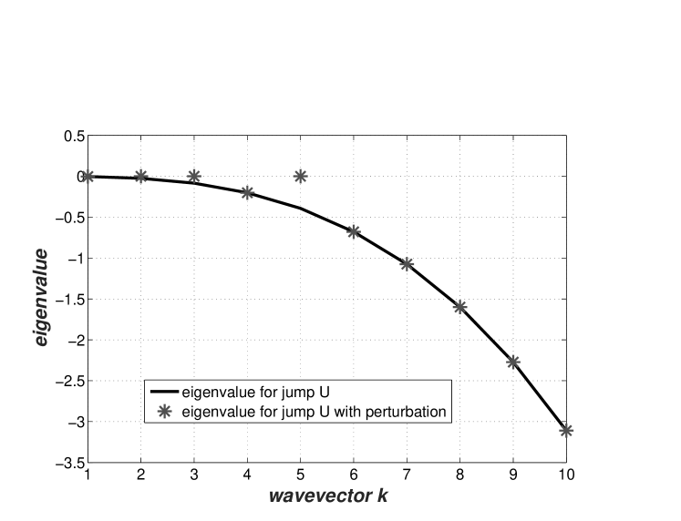
Figure 4: This plot show the roots $\lambda$ of the equation for the profile $U$ close to a step function. The continuous curve shows $\lambda(k)$ for $U=H(y-z0)$ where $z_{0}=0.0008$. The starred curve shows $\lambda(k)$ for a specially perturbed $U$, where $k_{1}=1,k_{2}=2,k_{3}=3,k_{4}=5$.

The proof can be found in the Appendix. In the coming subsection we consider eigenfunctions of the operator $L$ and the conjugate operator involved in the normal form.

4.3 Eigenfunctions of $L$ with zero eigenvalues

Let us consider the eigenfunctions $e_{k}$ of $L$ with the zero eigenvalues. We have $2N+1$ eigenfunctions including the trivial one $e_{0}=(0,1)$. All the other eigenfunctions have the form

$$e_{k}(x,y)=\exp(ikx)(\omega_{k}(y),\theta_{k}(y))^{tr},$$ (4.61)

$$e_{-k}=\exp(-ikx)(\omega_{-k}(y),\theta_{-k}(y))^{tr},$$ (4.62)

where $k\in\{k_{1},k_{2},...,k_{N}\}$ and

$$\omega_{k}=ikA_{k}\frac{\sinh(k(h-y))}{\sinh(kh)},\quad i=\sqrt{-1},$$ (4.63)

$$\theta_{k}=A_{k}\Theta_{k}(y),$$ (4.64)

where $A_{k}(\nu)$ are constants.

To obtain real value eigenfunctions, we take real and imaginary parts of these complex eigenfunctions. The real parts of the eigenfunctions, where $\omega_{k},\theta_{k}$ are proportional to $\sin(kx),\ \cos(kx)$ respectively, are denoted by the upper index $+$, and the imaginary parts, where $\omega_{k},\theta_{k}$ are proportional to $\cos(kx),\ \sin(kx)$, are denoted by the upper index $-$. The real eigenfunctions of $L$ have the form

$$e_{k}^{+}=(\omega_{k}(y)\sin(kx),\theta_{k}(y)\cos(kx))^{tr},$$ (4.65)

$$e_{k}^{-}=(-\omega_{k}(y)\cos(kx),\theta_{k}(y)\sin(kx))^{tr}.$$ (4.66)

Respectively, the real eigenfunctions of formally conjugate operator $L^{*}$ are

$$\tilde{e}_{k}^{+}=(\tilde{\omega}_{k}(y)\sin(kx),\tilde{\theta}_{k}(y)\cos(kx))^{tr},$$ (4.67)

$$\tilde{e}_{k}^{-}=(-\tilde{\omega}_{k}(y)\cos(kx),\tilde{\theta}_{k}(y)\sin(kx))^{tr}.$$ (4.68)

We have the relations

$$\tilde{\theta}_{k}^{+}=a_{k}\cosh(k(h-y)),\quad$$ (4.69)

where $a_{k}$ are coefficients. One can show that there exist no generalized eigenfunctions of the operator $L$ [11].

In the remaining part of this paper we describe a formal mathematical realization of the key point iii, i.e. a control of the normal form that determine the dynamics at the bifurcation point. That control is based on the method of realization of vector fields (RVF) (see Appendix).

5 Normal form at the bifurcation point

Assume that $\gamma>0$ is a small parameter, and $|b-b_{c}|<\gamma^{2}$, i.e., we are seeking solutions at the bifurcation point. In this section, we reduce the Navier-Stokes dynamics to a system of ordinary differential equations. This reduction is standard and follows from known works [6].

Let $E_{N}$ be the finite dimensional subspace $E_{N}=Span\{e_{0},e_{1}^{+},...,e_{N}^{+},e_{1}^{-},...,e_{N}^{-}\}$ of the phase space ${\mathcal{H}}$, where $e_{j}^{\pm}=(\omega_{j}^{\pm},\theta_{j}^{\pm})^{tr}$ are the eigenfunctions of the operator $L$ with zero eigenvalues. Let ${\bf P}_{N}$ be a projection operator on $E_{N}$ and ${\bf Q}_{N}={\bf I}-{\bf P}_{N}$. The components of ${\bf P}_{N}$ are defined by

$${\bf P}_{1,N}v=\sum_{j=1}^{N}\langle\tilde{\omega},\tilde{\omega}_{j}^{+}\rangle\omega_{j}^{+}+\sum_{j=1}^{N}\langle\tilde{\omega},\tilde{\omega}_{j}^{-}\rangle\omega_{j}^{-},$$ (5.70)

$${\bf P}_{2,N}v=(2\pi h)^{-1}\langle w,1\rangle+\sum_{j=1}^{N}\langle w,\tilde{\theta}_{j}^{+}\rangle\theta_{j}^{+}+\sum_{j=1}^{N}\langle w,\tilde{\theta}_{j}^{-}\rangle\theta_{j}^{-},$$ (5.71)

where $v=(\tilde{\omega},w)^{tr}$ and $\tilde{e}_{j}^{\pm}=(\tilde{\omega}_{i}^{\pm},\tilde{\theta}_{i}^{\pm})$ are eigenfunctions of the conjugate operator $L^{*}$ with zero eigenvalues $\lambda=0$ found above (see subsection 4.3).

First we transform equations (3.24)-(3.25) to a standard system with ”fast” and ”slow” modes. Let us introduce auxiliary functions $R_{\omega}(X)$, $R_{\psi}(X)$ and $R_{w}(X)$ by

$$R_{\omega}(X)=\sum_{j=1}^{N}X_{j}^{+}\omega_{j}^{+}+\sum_{j=1}^{N}X_{j}^{-}\omega_{j}^{-},\quad R_{\psi}(X)=\sum_{j=0}^{N}X_{j}^{+}\psi_{j}^{+}+\sum_{j=1}^{N}X_{j}^{-}\psi_{j}^{-},$$

$$R_{w}(X)=X_{0}+\sum_{j=1}^{N}X_{j}^{+}\theta_{j}^{+}+\sum_{j=1}^{N}X_{j}^{-}\theta_{j}^{-},$$

and represent $\tilde{\omega},\tilde{\psi}$ and $w$ by

$$\tilde{\omega}=\tilde{\gamma}R_{\omega}(X)+\hat{\omega},\quad\quad\tilde{\psi}=\gamma R_{\psi}(X)+\hat{\psi},$$ (5.72)

$$w=\gamma R_{w}(X)+\hat{w},$$ (5.73)

where ${\bf P}_{N}(\hat{\omega},\hat{w})^{tr}=0,$ $X_{i}^{\pm}(t)$ and $\hat{\omega},\hat{w},\hat{\psi}$ are new unknown functions, $X=(X_{0},X_{1}^{+},...,X_{N}^{+},X_{1}^{-},...,X_{N}^{-})^{tr}$.

We substitute relations (5.72)-(5.73) in Eqs. (3.24) and (3.25). As a result, one obtains the system

$$\frac{dX_{i}^{\pm}}{dt}=\gamma^{-1}(G_{i}^{\pm}(X)+M_{i}^{\pm}(X)+f_{i}^{\pm}+F_{i}^{\pm}(X,\hat{\omega},\hat{w},\gamma)),$$ (5.74)

$$\hat{\omega}_{t}=\nu\Delta\hat{\omega}+{\bf P}_{1,N}F(X,\hat{\omega},\hat{w},\gamma),$$ (5.75)

$$\hat{w}_{t}=\Delta\hat{w}-\{\hat{\psi},U\}+{\bf P}_{2,N}G(X,\hat{\omega},\hat{w},\gamma),$$ (5.76)

where in Eqs.(5.75) and (5.76)

$$F=\{\gamma R_{\psi}(X)+\hat{\psi},\gamma R_{\omega}(X)+\hat{\omega}\},$$ (5.77)

$$G=\{\gamma R_{\psi}(X)+\hat{\psi},\gamma R_{w}(X)+\gamma u_{1}+\hat{w}\}+\gamma^{2}\eta_{1}.$$ (5.78)

The functions $G_{i}^{\pm}(X)$ and $M_{i}^{\pm}(X)$ give main contributions in the right hand sides of Eqs.(5.74) and $F_{i}^{\pm}$ are corrections defined by

$$F_{i}^{\pm}=\gamma^{-1}(F_{i}^{\pm,\omega}+F_{i}^{\pm,w}),$$ (5.79)

where

$$F_{i}^{\pm,\omega}=\langle\{\gamma R_{\psi}(X),\hat{\omega}\}+\{\hat{\psi},\gamma R_{\omega}(X)+\hat{\omega}\},\tilde{\omega}_{i}^{\pm}\rangle,$$

$$F_{i}^{\pm,w}=\langle\{\gamma R_{\psi}(X),\hat{w}\}+\{\hat{\psi},\gamma R_{w}(X)+\gamma u_{1}+\hat{w}\},\tilde{\theta}_{i}^{\pm}\rangle).$$

One has

$$G_{i}^{\pm}(X)=\langle\{R_{\psi}(X),R_{w}(X)\},\tilde{\theta}_{i}^{\pm}\rangle+\langle\{R_{\psi}(X),R_{\omega}(X)\},\tilde{\omega}_{i}^{\pm}\rangle,$$

$$M_{i}^{\pm}(X)=\langle\{R_{\psi}(X),u_{1}\},\tilde{\theta}_{i}^{\pm}\rangle.$$

These terms can be rewritten in a more explicit form as

$$G_{i}^{+}(X)=\sum_{j,l=1}^{N}G_{ijl}^{+++}X_{j}^{+}X_{l}^{+}+G_{ijl}^{--+}X_{j}^{-}X_{l}^{-},$$ (5.80)

$$G_{i}^{-}(X)=\sum_{j,l=1}^{N}G_{ijl}^{+--}X_{j}^{+}X_{l}^{-}$$ (5.81)

and

$$M_{i}^{+}(X)=\sum_{j=1}^{N}M_{ij}^{++}X_{j}^{+}+\sum_{j=1}^{N}M_{ij}^{+-}X_{j}^{-},$$ (5.82)

$$M_{i}^{-}(X)=\sum_{j=1}^{N}M_{ij}^{-+}X_{j}^{+}+\sum_{j=1}^{N}M_{ij}^{--}X_{j}^{-}.$$ (5.83)

Note that in Eqs. (5.80) - (5.83) all the other possible terms vanish since they are defined by integrals over $x$ of functions odd in $x$. The coefficients in (5.80),(5.81), (5.82) and (5.83) are defined by

$$M_{ij}^{\pm\pm}(u_{1})=\langle\{\psi_{j}^{\pm},\tilde{\theta}_{i}^{\pm}\},u_{1}\rangle,$$ (5.84)

$$G_{ijl}^{+++}=\langle\{\psi_{j}^{+},\theta_{l}^{+}\},\tilde{\theta}_{i}^{+}\rangle+O(\nu^{-1})$$ (5.85)

$$G_{ijl}^{--+}=\langle\{\psi_{j}^{-},\theta_{l}^{-}\},\tilde{\theta}_{i}^{+}\rangle+O(\nu^{-1})$$ (5.86)

$$G_{ijl}^{+--}=\langle\{\psi_{j}^{+},\theta_{l}^{-}\}+\{\psi_{l}^{-},\theta_{j}^{+}\},\tilde{\theta}_{i}^{-}\rangle+O(\nu^{-1})$$ (5.87)

for large $\nu$. These estimates are obtained in [11] by expressions for conjugate eigenfunctions. One has

$$f_{i}^{\pm}=\langle\eta_{1},\tilde{\theta}_{i}^{\pm}\rangle.$$ (5.88)

We consider Eqs.(5.74), (5.75) and (5.76) in the domain

$$D_{\gamma,R,C_{1},C_{2}}=\{(X,\hat{w},\hat{\omega}):\ |X|<R,\ ||\hat{\omega}||_{\alpha}<C_{1}\gamma^{2},||\hat{w}||_{1+\alpha}<C_{2}\gamma^{2}\},$$ (5.89)

where $\alpha>3/4$. Using results [11], one can prove the following assertion describing the normal form of dynamics in a small neighborhood of the bifurcation point.

Lemma 5.1

Let $r\in(0,1)$ and $|b-b_{c}|<\gamma^{2}$. Assume $\gamma>0$ is small enough: $\gamma<\gamma_{0}(N,\nu,R,r).$ Then the local semiflow $S^{t}$, defined by equations (5.74),(5.75), and (5.76) has a locally invariant and locally attracting manifold ${\mathcal{M}}_{2N+1,\gamma}$. This manifold is defined by

$$\hat{\omega}=\hat{\omega}_{0}(X,\gamma),\quad\hat{w}=\hat{w}_{0}(X,\gamma),$$ (5.90)

where $\hat{\omega}_{0}(X,\gamma)$, $\hat{w}_{0}(X,\gamma)$ are maps from the ball ${\mathcal{B}}^{2N+1}(R)=\{X:|X|<R\}$ to $H_{\alpha}$ and $H_{1+\alpha}$ respectively, bounded in $C^{1+r}$ -norm :

$$|\hat{\omega}_{0}(X,\gamma)|_{C^{1+r}({\mathcal{B}}^{2N+1}(R))}<C_{3}\gamma^{2},\quad|\hat{w}_{0}(X,\gamma)|_{C^{1+r}({\mathcal{B}}^{2N+1}(R))}<C_{4}\gamma^{2}.$$ (5.91)

The restriction of the semiflow $S^{t}$ on ${\mathcal{M}}_{2N+1,\gamma}$ is defined by

$$\frac{dX_{i}^{\pm}}{dt}=\gamma(G_{i}^{\pm}(X)+M_{i}^{\pm}(X)+f_{i}^{\pm})+\phi_{i}^{\pm}(X,\gamma)),$$ (5.92)

$$\frac{dX_{0}}{dt}=0,$$ (5.93)

and the corrections $\phi_{i}^{\pm}(X,\gamma)=F_{i}^{\pm}(X,\hat{\omega}_{0}(X,\gamma),\hat{w}_{0}(X,\gamma),\gamma)$ satisfy the estimates

$$|\phi_{i}^{\pm}|,|D_{X}\phi_{i}^{\pm}|<c_{1}\gamma^{s},\quad s>0.$$ (5.94)

Our aim in coming sections is to prove that the normal forms (5.92) exhibit very complex dynamics. To be precise this assertion let’s us formulate the definition.

Definition Consider a family of the semiflows $S^{t}(P)$, where $P$ is a parameter, defined on Banach space $H$. If this family $\epsilon$- realizes (in the sense of subsection 8.2) all smooth finite dimensional systems with arbitrarily prescribed accuracy $\epsilon>0$ then we say that family is is maximally dynamically complex.

The meaning of this definition is that maximally dynamically complex systems can generate all kinds of structurally stable dynamics, in particular, all hyperbolic dynamics. Such dynamics may be chaotic (as examples, we can take Anosov’s flows, homoclinic chaos and others [7, 24]). To formulate an important property of maximally dynamically complex systems, let us denote by ${B}^{n}(R)$ be the ball $\{q:|q|\leq R\}$ in ${\bf R}^{n}$ of the radius $R>0$ centered at $0$, where $q=(q_{1},q_{2},...,q_{n})$ and $|q|^{2}=q_{1}^{2}+...+q^{2}_{n}$ and consider a system of differential equations on the ball ${B}^{n}(R)$:

$$\frac{dq}{dt}=Q(q),$$ (5.95)

where

$$Q\in C^{1}({B}^{n}),\quad\sup_{q\in{B}^{n}(R)}|\nabla Q(q)|<1.$$ (5.96)

Suppose the vector field $Q$ is directed strictly inward to the ball ${B}^{n}(R)$ at its boundary $\partial{B}^{n}(R)=\{q:|q|=R\}$:

$$Q(q)\cdot q<0\quad for\ q\in\partial{B}^{n}(R).$$ (5.97)

Then Eq. (5.95) defines a finite dimensional global semiflow on ${B}^{n}(R)$. Now we can formulate

Proposition. If a family of the semiflows is maximally dynamically complex, then these semiflows enjoy the following property. For each integer $n$, each $\epsilon>0$ and each vector field $Q$ satisfying (5.96) and (5.97) and having a hyperbolic dynamics $G_{\Gamma}^{t}$ on a compact invariant hyperbolic set $\Gamma$, there exists a value of the parameter $\mathcal{P}$ such that the corresponding system (6.98) defines a semiflow $S^{t}_{\mathcal{P}}$, which also has a hyperbolic dynamics $G_{\Gamma^{\prime}}^{t}$ on a hyperbolic set $\Gamma^{\prime}$, which is homeomorphic to $\Gamma$. The dynamics $G_{\Gamma^{{}^{\prime}}}^{t}$ and $G_{\Gamma}^{t}$ are orbitally topologically equivalent.

For definitions of hyperbolic sets, dynamics and orbital topological equivalence see, for example, [7, 24] among others.

The proof of this claim (see [9]) uses the theorem on persistence of hyperbolic sets [24]. According to this theorem, we can choose a sufficiently small $\epsilon(Q,\Gamma)>0$ such that if estimate (8.160) holds then system (8.159) has a compact invariant hyperbolic set $\Gamma^{\prime}$ homeomorphic to $\Gamma$ and, moreover, the global semiflows defined by systems (5.95) and (8.159) generate orbitally topologically equivalent dynamics on invariant sets $\Gamma$ and $\Gamma^{{}^{\prime}}$, respectively.

The theory of maximally dynamical complex systems is based on the RVF method (on the RVF method see Appendix, subsection 8.2) and it is developed for neural networks and reaction diffusion systems (see [9]). In this paper, we first state a hydrodynamical example.

In the next section we apply the RVF method for quadratic systems (5.92). As a parameter $P$ we use the function $u_{1}(x,y)$, i.e., a small two dimensional spatial inhomogeneity. The matrix $M^{\pm}$ in the right hand side of (5.92) is a linear functional of $u_{1}$. One can show (see [11]) that, by adjusting $u_{1}$, we can obtain any matrices $M^{\pm}$. This assertions seems natural since the matrices $M^{\pm}$ contain $N^{2}$ entries, thus we should satisfy $N^{2}$ restrictions by an infinite set of unknowns, which are the Fourier coefficients of $u_{1}$.

So, the matrix $M^{\pm}$ in normal forms (5.92) can take any values, however, the main difficulty is that the quadratic terms in the normal forms (5.92) are not arbitrary and subject some restrictions. Our plan to overcome this difficulty is as follows. We use the key auxiliary assertion, Lemma 6.2, which means that any given quadratic system can be realized by a normal form (5.92) of a sufficiently large dimension $N$.

6 Reductions of quadratic systems

Our next step is to study a general class of quadratic systems, which includes (5.92) as a particular case. We consider the following systems

$$\frac{dX}{dt}={K}(X)+{M}X+g,$$ (6.98)

where $X=(X_{1},...,X_{N}),\ {K}=(K_{1},...,K_{N}),{g}=(g_{1},...,g_{N})\in{\bf R}^{N}$, $K(X)$ is a quadratic map defined by

$${K}_{i}(X)=\sum_{j=1}^{N}\sum_{l=1}^{N}K_{ijl}X_{j}X_{l},$$

and $MX$ is a linear operator $({M}X)_{i}=\sum_{j=1}^{N}M_{ij}X_{j}.$ System (6.98) defines a local semiflow $S^{t}(g,{M})$ in the ball ${\mathcal{B}}^{N}(R_{0})\subset{\bf R}^{N}$ of the radius $R_{0}$ centered at $0$. We shall consider the vector $g$ and the matrix $M$ as parameters of this semiflow whereas the entries $K_{ijl}$ will be fixed.

Let us formulate an assumption on entries $K_{ijl}$. We present $X$ as $X=(Y,Z)$, where

$$Y_{l}=X_{i_{l}},\quad l\in I_{p},\quad Z_{l}=X_{j_{l}},\quad l\in J_{p},$$

where $I_{p}=\{i_{1},...,i_{p}\}$ and $J_{p}=\{j_{1},...,j_{N-p}\}$ are disjoint subsets of $\{1,...,N\}$ such that $I_{p}\cup J_{p}=\{1,...,N\}.$ Then system (6.98) can be rewritten as follows:

$$\frac{dY}{dt}={K}^{(1)}(Y)+{K}^{(2)}(Y,Z)+{K}^{(3)}(Z)+{R}Y+{P}Z+f,$$ (6.99)

$$\frac{dZ}{dt}=\tilde{K}^{(1)}(Y)+\tilde{K}^{(2)}(Y,Z)+\tilde{K}^{(3)}(Z)+\tilde{R}Y+\tilde{P}Z+\tilde{f},$$ (6.100)

where

$${K}^{(1)}_{i}(Y)=\sum_{j\in I_{p}}\sum_{l\in I_{p}}K_{ijl}^{(1)}Y_{j}Y_{l},\quad\tilde{K}_{k}^{(1)}(Y)=\sum_{j\in I_{p}}\sum_{l\in I_{p}}\tilde{K}_{kjl}^{(1)}Y_{j}Y_{l},$$ (6.101)

$${K}^{(2)}_{i}(Y,Z)=\sum_{j\in I_{p}}\sum_{l\in J_{p}}K_{ijl}^{(2)}Y_{j}Z_{l},\quad\tilde{K}_{k}^{(2)}(Y,Z)=\sum_{j\in I_{p}}\sum_{l\in J_{p}}\tilde{K}_{kjl}^{(2)}Y_{j}Z_{l},$$ (6.102)

$${K}^{(3)}_{i}(Z)=\sum_{j\in J_{p}}\sum_{l\in J_{p}}K_{ijl}^{(3)}Z_{j}Z_{l},\quad\tilde{K}_{k}^{(3)}(Z)=\sum_{j\in J_{p}}\sum_{l\in J_{p}}\tilde{K}_{kjl}^{(3)}Z_{j}Z_{l}$$ (6.103)

and where $i\in\{1,...,p\},\ k\in\{1,...,N-p\}$. Linear terms have the form

$$(\tilde{R}Y)_{i}=\sum_{j\in I_{p}}\tilde{R}_{ij}Y_{j},\quad(\tilde{P}Z)_{i}=\sum_{j\in J_{p}}\tilde{P}_{ij}{Z_{j}},\quad({P}Z)_{i}=\sum_{j\in J_{p}}P_{ij}Z_{j},$$ (6.104)

and $f=(f_{1},...,f_{p}),\ \tilde{f}=(\tilde{f}_{1},...,\tilde{f}_{N-p})$. We denote by $S^{t}({\mathcal{P}})$ the local semiflow defined by (6.99) and (6.100). Here ${\mathcal{P}}$ is a semiflow parameter, ${\mathcal{P}}=\{f,\tilde{f},{P},\tilde{P},{R},\tilde{R}\}$.

$p$-Decomposition Condition Suppose entries $K_{ijl}$ satisfy the following condition. For some $p$ there exists a decomposition $Z=(X,Y)$ such that for all numbers $b_{jl}$, where $j,l\in I_{p}$, the linear system

$$\sum_{i\in J_{p}}\tilde{K}_{ijl}^{(1)}u_{i}=b_{jl},\quad l,j\in I_{p}$$ (6.105)

has a solution $u$.

Clearly, for $N>p^{2}+p$ and generic matrices $K$ this condition is valid.

Let us formulate some conditions to the matrices ${R},\tilde{R},{P}$ and $\tilde{P}$. Let $\xi>0$ be a parameter. We suppose that

$$\tilde{P}_{ij}=-\xi^{-1}\delta_{ij},\quad i=1,...,N-p,\ j=1,...,$$ (6.106)

where $\delta_{ij}$ is the Kronecker symbol,

$$\tilde{R}_{ij}=0,\quad\tilde{f}_{i}=0,\quad i=1,...,N-p,\ j=1,...,p,$$ (6.107)

$$P_{ij}=\xi^{-1}T_{ij},\quad|T_{ij}|<C_{0},\quad i=1,...,p,\ j=1,...,N-p,$$ (6.108)

$$|R_{ij}|<C,\quad i=1,...,p,\ j=1,...,p,$$ (6.109)

Let us fix $p$ and consider the numbers $N,\xi$, coefficients $T_{ij},R_{ij}$ and $f_{i}$ as a parameter $P$.

Lemma 6.1

Assume (6.106), (6.107), (6.108) and (6.109) hold. For sufficiently small positive $\xi<\xi_{0}(R_{0},r,f)$ the local semiflow $S^{t}(P)$ defined by system (6.99), (6.100) has a locally invariant and locally attracting manifold ${\mathcal{M}}_{P}$. This manifold is defined by equations

$$Z=\xi(\tilde{K}^{(1)}(Y)+W(Y,\xi)),\quad Y\in{B}^{p}(R_{0})$$ (6.110)

where $W$ is a $C^{1}$ smooth map from the ball ${B}^{p}(R_{0})$ to ${\bf R}^{N-p}$ such that for some $C_{1},s>0$

$$|W(\cdot,\xi)|_{C^{1}({B}^{p}(R_{0}))}<C_{1}\xi^{s}.$$ (6.111)

Proof. Let us introduce a new variable $w$ by

$$Z=\xi(\tilde{K}^{(1)}(Y)+w).$$ (6.112)

and the rescaled time by $t=\xi\tau$. Then for $Y,w$ one obtains the following system

$$\frac{dY}{d\tau}=\xi G(Y,w,\xi),$$ (6.113)

$$\frac{dw}{d\tau}=\xi F(Y,w,\xi)-w,$$ (6.114)

where

$$G(Y,w,\xi)={K}^{(1)}(Y)+\xi{K}^{(2)}(Y,\tilde{K}^{(1)}(Y)+w)+$$

$$+\xi^{2}{K}^{(3)}(\tilde{K}^{(1)}(Y)+w)+{R}Y+{T}(\tilde{K}^{(1)}(Y)+w)+f,$$

$$F(Y,w,\xi)=\tilde{K}^{(2)}(Y,\tilde{K}^{(1)}(Y)+w)+$$

$$+\xi\tilde{K}^{(3)}(\tilde{K}^{(1)}(Y)+w)+h(Y,w,\xi),$$

$$h(Y,w,\xi)=-D_{Y}\tilde{K}^{(1)}(Y)G(Y,w,\xi).$$ (6.115)

Equations (6.113), (6.114) form a typical system involving slow ($Y$) and fast ($w$) variables. Existence of a locally invariant manifold for this system can be shown by the well-known results (see [21]). The remaining part of the proof is standard (see [11]) and is omitted $\square$.

The semiflow $S^{t}$ restricted to ${\mathcal{M}}$ is defined by the equations

$$\frac{dY}{dt}=F(Y,\xi),$$ (6.116)

where

$$F(Y,\xi)={K}^{(1)}(Y)+\xi{K}^{(2)}(Y,\tilde{K}^{(1)}(Y)+W(Y,\xi))+$$

$$+\xi^{2}{K}^{(3)}(\tilde{K}^{(1)}(Y)+W(Y,\xi))+{R}Y+{T}\tilde{K}^{(1)}(Y)+W(Y,\xi))+f.$$

The estimates for $W$ show that $F$ can be presented as

$$F(Y,\xi)={K}^{(1)}(Y)+{R}Y+{T}\tilde{K}^{(1)}(Y)+f+\phi_{\xi}(Y)$$ (6.117)

where a small correction $\phi_{\xi}$ satisfies

$$|\phi_{\xi}|_{C^{1}({B}^{p}(R_{0}))}<c_{0}\xi^{1/2}.$$ (6.118)

In (6.117) $R$ and $f$ are free parameters. The quadratic form ${D}(Y)={K}^{(1)}+{T}\tilde{K}^{(1)}$ can be also considered as a free parameter according to the $p$- Decomposition Condition. Therefore, we have proved the following assertion.

Lemma 6.2

Let

$$F(Y)={D}(Y)+{R}Y+f$$ (6.119)

be a quadratic vector field on ${\mathcal{B}}^{p}(R_{0})$, where

$${D}_{i}(Y)=\sum_{j=1}^{p}\sum_{l=1}^{p}D_{ijl}Y_{j}Y_{l},\quad({R}Y)_{i}=\sum_{j=1}^{p}R_{ij}Y_{j}.$$

Consider system (6.99), (6.100). Let the $p$- Decomposition Condition hold. Then for any $\epsilon>0$ the field $F$ can be $\epsilon$ - realized by the semiflow $S^{t}({\mathcal{P}})$ defined by system (6.99), (6.100), where parameters $\mathcal{P}$ are the dimension $N$, the matrices ${P}$, $R$, $\tilde{P}$, $\tilde{R}$ and the vectors $f,\tilde{f}$.

This lemma immediately follows from the main result on quadratic systems (6.98). Note that the class of systems (6.119) includes the Lorenz model as a particular case.

Theorem 6.3

Consider the family of semiflows defined by systems (6.98), where the triple $\{N,M,g\}$ serves as a parameter ${\mathcal{P}}$, and for each $N$ the coefficients $K_{ijl}$ with $i,j,l\in\{1,...,N\}$ satisfy $p$-decomposition condition for an integer $p$ such that $N/2<p^{2}+p\leq N$. Then that family is maximally dynamically complex .

Proof. According to results [8] for any $\epsilon_{1}>0$ we can construct $\epsilon_{1}$-realization of the field $Q$ by semiflows defined by (6.119). Moreover, due to the previous lemma, for any $\epsilon_{2}>0$ we can find $\epsilon_{2}$ -realization of any system (6.119) by semiflows defined by (6.98). If $\epsilon_{k}>0$ are small enough, these two realizations give us $\epsilon$-realization of $Q$. The corresponding system (6.98) has the hyperbolic set $\Gamma^{\prime}$. This completes the proof.

The last result show that quadratic systems (6.98), that arise as a result of our bifurcations, can exhibit all chaotic hyperbolic dynamics, for example, Anosov ś flows or axiom A Smale dynamics. To prove that such hyperbolic chaotic dynamics can be generated by the original Marangoni fluid dynamics (defined by IBVP (2.13)-(2.20)) we need additional technical assertions. They can be obtained following [11].

7 Concluding remarks

Bifurcations of fluid dynamics leading to periodic spatial patterns (for example, Bénard cells) or time periodic regimes are well studied. In 1971, Ruelle and Takens [3] pioneered the hypothesis that there are more complicated bifurcations possible, which describe a transition from a simple rest point attractor to strange attractors (which can describe a turbulence). However, until now there exists no completely analytical proof of the existence of such bifurcations. Note that turbulence exhibits not only complicated time dynamics, but complex spatial patterns are also observed.

This paper states a proof of existence of bifurcations, which can produce turbulence and complicated patterns. It is shown that, at the bifurcation point, the dynamics can be described by systems of differential equations with quadratic nonlinearities. Such systems can have chaotic dynamics, specifically, they can generate all finite dimensional hyperbolic dynamics.

Physically the complicated spatio-temporal patterns are generated by diffusion, convection, and the capillary effect. The fact that the Marangoni effect can induce an interfacial turbulence has been long known from experiments and numerical simulations (see, for example, [25, 26]). In our model, the physical mechanism of this phenomenon is an interaction of slow modes which determine the dynamics and the spatial inhomogeneities in the system.

We think that this mechanism is also applicable for climate models. Indeed, climate systems always include slow and fast components. Therefore, in the climate models there are internal interactions between the slow segments of the climate system and the fast weather components. The results of this paper show that these interactions can lead to different variants of complex dynamics. We have a new physical mechanism for the generation of complicated dynamics. Namely, it is shown that in spatially extended systems with many slow variables different small inhomogeneities can lead to sharply different dynamics, which may be chaotic. Mathematically it can be shown by the method of realization of vector fields, however, the physical idea behind this method is transparent. In fact, in spatially extended systems the number of slow modes usually is much smaller than the number of the fast ones. Some space inhomogeneities define an interaction between the fast and slow modes. We have thus a number of parameters which affect the dynamics of the slow variables and which can be used to control those dynamics.

8 Appendix

                                                                                                  

8.1 Proof of Theorem 4.2

Proof. First we use Lemma 4.1 to obtain a nonlinear equation for the eigenvalues $\lambda(k)$ of the boundary value problem (4.38)-(4.40). As a result, one has

$$k^{2}\nu\lambda^{-1}D^{-1}\beta_{k}\int_{0}^{h}\Phi_{k}(y,\lambda)\psi_{k}(y,\lambda)\rho_{\bar{k}}(y)U_{y}(y,\nu)dy=b^{-1}\beta_{k}(\lambda).$$ (8.120)

Note that the operator $L$ is not self-adjoint. Therefore, complex eigenvalues $\lambda$ may appear, i.e., complex roots of (8.120). Moreover, let us note that, according to (4.43), if $\beta_{k}(\lambda)=0$, then Eq. (8.120) is satisfied. In this case (4.38) entails that

$$\frac{d^{2}\omega_{k}(y)}{dy^{2}}-k_{\nu}^{2}\omega_{k}=0,\quad\omega_{k}(h)=0,\quad\omega_{k}(0)=0,$$ (8.121)

therefore $k_{\nu}^{2}=-(n\pi/h)^{2}$, where $n$ is an integer. This gives $\lambda=-\nu((n\pi/h)^{2}+k^{2})<-1/2$. These eigenvalues $\lambda$ correspond to trivial solutions of the eigenfunction problem with $\lambda\notin{\bf C}_{1/2}$. Therefore, without loss of generality we can set $\beta_{k}(\lambda)=1$ in Eq.(8.120).

The plan of the remaining part of the proof is as follows. We consider the two cases: $({\bf I})\hskip 2.84544pt|\lambda|<\nu^{3/4}$ and $({\bf II})\hskip 2.84544pt|\lambda|>\nu^{3/4}.$ In the first case we can simplify equation (8.120), while in the second case a rough estimate shows that Eq. (8.120) has no solutions.

Let us start with the case I. To simplify our statement, we first consider a formal limit of Eq.(8.120) as $\nu\to+\infty$. Using (4.50), (4.51) and (4.56) one obtains that this limit has the form

$$(2\bar{D})^{-1}\int_{0}^{+\infty}y\bar{U}_{y}(y)\exp(-(k+\bar{k})y)dy=\bar{k}/k,\quad\bar{D}=Db^{-1},$$ (8.122)

where $\bar{U}$ is the limit $\bar{U}=\lim U_{K_{N}}(y,\nu)$ as $\nu\to+\infty$ (it will be shown below that this limit exists). We set $\bar{U}=V(y,d)$, where $V$ is a function of a special form that depends on some parameters $d=(d_{1},...,d_{M})$, where $M=k_{N}$. Consider $C^{\infty}$ - mollifiers $\delta_{\epsilon}(y)$ such that $\delta_{\epsilon}\geq 0$, the support $supp\ \delta_{\epsilon}(y)$ is $(-\epsilon,\epsilon)$ and

$$\int_{-\epsilon}^{\epsilon}\delta_{\epsilon}(y)dy=1,$$ (8.123)

$$\sup|D_{y}^{k}\delta_{\epsilon}(y)|<c_{k}\epsilon^{-(k+1)},\quad k=0,1,2.$$ (8.124)

Let us define the function $V(y,d)$ on $[0,\infty)$ by

$$V_{y}(y,d)=2y^{-1}(\delta_{\kappa}(y-z_{0})+\mu yP_{M}(y,d)),$$ (8.125)

where $\chi(z)$ is the step function such that $\chi(z)=1$ for $z>0$ and $\chi(z)=0$ for $z<0$, $P_{M}$ is a polynomial in $y$ of the degree $M+1$ with coefficients depending on $(d_{1},d_{2},...,d_{M})$, and

$$\mu=\kappa^{2/3},\quad z_{0}=5\kappa,$$ (8.126)

where $\kappa$ is a small parameter independent of $\nu$ and $\gamma$. Assume that coefficients of the polynomial $P_{M}$ and $d_{j}$ are bounded:

$$P_{M}(y,d)=\sum_{j=0}^{M}b_{j}(d)y^{j},\quad|b_{j}(d)|<C,\quad|d_{j}|<1/2.$$ (8.127)

To investigate (8.122) it is useful to introduce the variable

$$p=k+\bar{k}=k+(k^{2}+\lambda)^{1/2}.$$ (8.128)

Then Eq. (8.122) can be rewritten as

$$\bar{D}\frac{p}{k}=1+\bar{D}+S(p,k,d),$$ (8.129)

where

$$S(p,k,d)=\mu G(p,d)+g_{\kappa}(p),$$ (8.130)

$$g_{\kappa}(p)=-1+\int_{0}^{\infty}\delta_{\kappa}(y-z_{0})\exp(-py)dy,$$ (8.131)

and

$$G(p,d)=\int_{0}^{\infty}yP_{M}(y,d)\exp(-py)dy.$$ (8.132)

We suppose that $\bar{k}>0$ thus $Re\ p>k$. Therefore, we can investigate (8.129) in the domain

$${\bf C}_{1/2,k}=\{p\in{\bf C}:\ p=\sqrt{k^{2}+\lambda}+k,\ Re\ \lambda>-1/2,\ Re\ p>k\}.$$ (8.133)

Note that

$$Re\ p=k+\sqrt{k^{2}+Re\lambda+(Im\ p)^{2}},$$ (8.134)

this shows that in ${\bf C}_{1/2,k}$ we have $Re\ p>2k-1/2$. We also assume

$$|\bar{D}-1|\leq\kappa.$$ (8.135)

Taking into account this restriction to $\bar{D}$, we define the interval $J=(b_{1},b_{2})$ and $b_{c}$ by

$$b_{1}=\bar{D}^{-1}(1-\kappa),\quad b_{2}=\bar{D}^{-1}(1+\kappa),\quad b_{c}=\bar{D}^{-1}.$$ (8.136)

We can choose a polynomial $P_{M}$ such that

$$G(p,d)=p^{-2}(-1)^{M+1}\prod_{j=1}^{M}(\frac{1}{p}-\frac{1}{2j+d_{j}}).$$ (8.137)

Let us formulate an auxiliary assertion.

Lemma 8.1

One has

$$Re\ g_{\kappa}(p)\leq-\min\{2\kappa Re\ p,\quad 1/2\}.$$ (8.138)

Proof. Estimate (8.138) follows from (8.126) and (8.131). Indeed, due to (8.123) we have

$$Re\ g_{\kappa}(p)=\ \int_{0}^{h}\delta_{\kappa}(y-z_{0})(Re\ \exp(-py)-1)dy\leq$$

$$\leq\int_{0}^{h}\delta_{\kappa}(y-z_{0})(\exp(-Re\ p\ y)-1)dy$$

that according to (8.126) gives

$$Re\ g_{\kappa}(p)<\exp(-4\kappa Re\ p)-1.$$ (8.139)

Consider the function $J(x)=\exp(-x)-1$. By the Taylor series we obtain that $J(x)\leq-x+x^{2}/2$ for $x\geq 0$. This shows that $J(x)\leq-1/2$ for $x>1$ and $J(x)\leq-x/2$ for $x\in[0,1)$. These inequalities and (8.139) imply (8.138) $\square$.

Let us show that in the case $|p|>\kappa^{-3/4}$, under assumption (8.135), Eq. (8.129) has no solutions with $Re\lambda>-c_{0}\kappa$.

Lemma 8.2

If $|p|>\kappa^{-3/4}$ then for sufficiently small $\kappa$ solutions of (8.129) satisfy

$$Re\ p<2k-c_{4}k^{2}\kappa^{1/4},\quad c_{4}>0.$$ (8.140)

For the corresponding $\lambda_{k}(p)$ one has

$$Re\ \lambda_{k}<-c_{5}k^{2}\kappa^{1/4},\quad c_{5}>0.$$ (8.141)

Proof. Relation (8.134) shows that for $p\in{\bf C}_{1/2,k}$ one has $Re\ p>Im\ p$, thus $|p|>\kappa^{-3/4}$ entails $4Re\ p>\kappa^{-3/4}$. Then estimate (8.138) implies $Re\ g_{\kappa}(p)<-c_{2}\kappa^{1/4}.$ Moreover, $\mu Re\ G(p,d)<-c_{3}\mu.$ These estimates and condition (8.135) entail that for small $\kappa$ one has $Re\ S(p,k,d)<-c_{4}\kappa^{1/4}$ and, therefore, (8.140) holds. By (8.134) this gives us (8.141). $\square$

Consider the case $|p|<\kappa^{-3/4}$. Let us introduce a new unknown $\tilde{p}$ by $(2+\tilde{p})k=p.$ Then equation (8.129) can be rewritten as

$$\tilde{p}=H(\tilde{p},k,\bar{D}),$$ (8.142)

where

$$H(\tilde{p},k,\bar{D})=\bar{D}^{-1}(g_{\kappa}((2+\tilde{p})k)+\mu G((2+\tilde{p})k,d))+\bar{D}^{-1}-1.\quad$$ (8.143)

Let us prove an estimate of solutions to (8.142).

Lemma 8.3

In the domain ${\mathcal{D}}_{\kappa,k}=\{p:p\in{\bf C}_{1/2,k},\ |p|<c_{1}\kappa^{-3/4}\}$ solutions of (8.142) satisfy

$$|\tilde{p}|<C_{1}\kappa^{1/4},\quad C_{1}>0.$$ (8.144)

Proof. To prove this lemma, we note that if $p\in{\mathcal{D}}_{\kappa,k}$ then by (8.130),(8.131), and (8.132) one has

$$|g_{\kappa}(p)|<C_{2}\kappa^{1/4},\quad|G(p,d)|<C_{3}.$$ (8.145)

Therefore, using (8.135) and (8.126) one obtains

$$|H(\tilde{p},k)|<C_{5}(\mu+\kappa^{1/4}).$$ (8.146)

Now (8.142) shows that $\tilde{p}$ satisfies (8.144) $\square$.

Let us consider equation (8.142). Using the last lemma we note that, to resolve this equation, we can apply a perturbation theory. Relations (8.130), (8.131), and (8.137) show that in the domain ${\mathcal{D}}_{\kappa,k}$ one has

$$|\frac{\partial H(\tilde{p},k)}{\partial\tilde{p}}|<C_{6}\mu$$

for $p$ satisfying (8.144). Now Lemma 8.3 and the implicit function theorem entail that for sufficiently small $\kappa$ all roots $\tilde{p}$ of eq. (8.142) lie in ${\mathcal{D}}_{\kappa,k}$ and can be found by contracting mappings. For each fixed $k$ the solution $\tilde{p}_{k}$ of eq. (8.142) is unique in ${\mathcal{D}}_{\kappa,k}$.

Let us set

$$\tilde{p}_{k}^{*}=-\kappa,\quad k\in\{1,...,M\},\ and\ k\neq k_{j},$$ (8.147)

and

$$\tilde{p}_{k}^{*}=0,\quad k=k_{j},\quad j=1,...,N.$$ (8.148)

Lemma 8.4

Let us define $b_{1}$, $b_{2}$ and $b_{c}$ by (8.136). Then for sufficiently small $\kappa$ we can choose $d_{j}$, $j=1,...,M$, such that $|d_{j}|<1/2$ and:

A) for each $k\in\{1,...,M\}$ and $b=b_{c}$ eq. (8.142) has a unique solution $\tilde{p}=\tilde{p}_{k}^{*}$;

B) for $k=k_{j}$, $j=1,...,N$ one has $\tilde{p}_{k}(b_{c})=0$ and roots $\tilde{p}_{k}(b)$ change their signs at $b=b_{c}$ as $b$ goes through the interval $(b_{1},b_{2})$;

C) for $k>M$ and $b\in(b_{1},b_{2})$ solutions $\tilde{p}_{k}$ of eq. (8.142) satisfy

$$\tilde{p}_{k}<-c\kappa^{s},\quad s>0.$$

Proof. Let us fix $k\in\{1,...,M\}$ and consider $p\in{\mathcal{D}}_{\kappa,k}$, i.e., $p$ close to $2k$. Then for $\tilde{p}$ satisfying (8.144) from (8.137) we obtain the following asymptotic for $\tilde{G}(\tilde{p},d)=G((2+\tilde{p})k,d)$:

$$\tilde{G}(\tilde{p},d)=(-1)^{M+1}(\bar{a}_{k}+\tilde{a}_{k}(\tilde{p},d))(d_{k}-k\tilde{p}),$$

where

$$\bar{a}_{k}=(4k^{2})^{-2}\prod_{j=1,j\neq k}^{M}(\frac{1}{2k}-\frac{1}{2j}),$$

and $\tilde{a}_{k}(\tilde{p},d)$ is an analytic function such that $|\tilde{a}_{k}|=O(|\tilde{p}|+|d|)$ for small $\tilde{p},d$. Therefore, eq. (8.142) can be transformed to the form

$$\tilde{p}=R_{k}(\tilde{p},d,\kappa)+\mu(-1)^{M+1}\bar{a}_{k}d_{k},$$ (8.149)

where $R_{k}$ is an analytic function of $\tilde{p}$ and $d$ for small $|\tilde{p}|,|d|$ such that

$$\sup_{\tilde{p}_{k},d:|d|<\mu^{1/2},\tilde{p}_{k}\in{\mathcal{D}}_{\kappa,k}}(|R_{k}|+|grad_{\tilde{p}}R_{k}|)<c_{1}\kappa,$$

for some $c_{1}>0$. Therefore, for small $\kappa$ we can apply the Implicit Function Theorem to find $d_{j}$, $j=1,...,M$ such that the root $\tilde{p}_{k}$ of (8.149) satisfies condition (A). The assertion B) also follows from equation (8.149).

To prove assertion (C), let us consider an estimate of $Re\ \tilde{p}$ for $k>k_{N}$. We observe that for $k>k_{N}$ and $\tilde{p}$ satisfying (8.144) we have $\mu Re\ G<-c_{2}\kappa^{2/3}$, $Re\ g_{\kappa}(p)<-c\kappa$, and thus using (8.135) and eq. (8.142) we obtain $Re\ \tilde{p}<-c_{2}k\kappa^{2/3}$. $\square$.

Finally, we have obtained needed estimates of solutions (8.120) for the case I, $\beta_{k}=1$ and $\nu=+\infty$. To finish our investigation of Eq.(8.120) for the case of large $\nu$, we compare Eqs. (8.120) and its formal limit (8.122). We assume that the function $U=V(y,d)$ is defined as above, by (8.125).

We observe that for $\beta_{k}=1$ Eq. (8.120) can be rewritten as

$$\int_{0}^{+\infty}k\bar{k}^{-1}(\lambda)yV(y,d)\exp(-(k+\bar{k}(\lambda))y)dy=2\bar{D}-W_{k}(\lambda,\nu,d),$$ (8.150)

where $W_{k}=I_{k}+J_{k}$ and

$$I_{k}=k^{2}\int_{h}^{+\infty}\bar{\psi}_{k}(y,\lambda)\bar{\rho}_{\bar{k}}V_{y}(y,d)dy,$$ (8.151)

$$J_{k}=-k^{2}\int_{0}^{h}(\psi_{k}(y,\lambda)\rho_{\bar{k}}-\bar{\psi}_{k}(y)\bar{\rho}_{\bar{k}})V_{y}(y,d)dy.$$ (8.152)

Under assumption (4.41), $\lambda<<\nu^{s}$ for $s\in(0,1)$ and for sufficiently large $\nu$ the term $I_{k}$ satisfies the estimate

$$|I_{k}|<c_{1}k^{2}h^{M+3}\exp(-kh)<c_{2}\nu^{-4},$$ (8.153)

which is uniform in $k$. To estimate $J_{k}$ we use the inequality

$$|J_{k}|\leq k^{2}\int_{0}^{h}(|(\psi_{k}(y,\lambda)-\bar{\psi}_{k}(y))\rho_{\bar{k}}|+|\bar{\psi}_{k}(y)(\bar{\rho}_{\bar{k}}(y)-\rho_{k}(y))|)|V_{y}(y,d)|dy.$$ (8.154)

Now we apply relations (4.50), (4.56), estimate (4.49) and

$$\sup_{y\in[0,h]}|V_{y}(y,d)|<c_{3}(\kappa^{-2}+h^{M+3}).$$

Then we find that

$$|J_{k}|<c_{4}k^{2}(\kappa^{-2}+h^{M+3})(k^{2}\bar{k}^{-1}\exp(-\bar{k}h)+k\bar{k}^{-1}\lambda\nu^{-1})<$$

$$<c_{5}(1+\kappa^{-2})\nu^{s-1}$$

for some $s\in(0,1)$ and $c_{5}>0$. Note that in this estimate the constant $c_{5}$ is uniform in $k$. As a result, we obtain the estimate

$$|W_{k}(\lambda,\nu,d)|<c_{6}\kappa^{-2}\nu^{s-1},$$ (8.155)

which is uniform in $k$. Therefore, all analysis of (8.150) can be made the same arguments as above that allows us to prove the next lemma.

Lemma 8.5

Let assumptions (4.41) hold, $N$ be a positive integer and $K_{N}=\{k_{1},...,k_{N}\}$ be a subset of ${\bf Z}_{+}$ and $V(y,d)$ is defined by (8.125). Moreover, let $|\lambda|<\nu^{3/4}$. Then in relation (8.125) we can choose parameters $\kappa$ and $d$ such that for sufficiently large $\nu$ the roots $\lambda(k,b,\nu)$ of equation (8.150), which lie in the domain $|\lambda|<\nu^{3/4}$, satisfy

(i )

$$\lambda(k,b_{c},\nu)=0\quad k\in K_{N},$$ (8.156)

and

$$Re\ \lambda(k,b_{c},\nu)<-\delta_{N}\quad k\notin K_{N},$$ (8.157)

where positive $\delta_{N}$ is uniform in $\nu$ as $\nu\to\infty$;

(ii) for $k\in K_{N}$ the eigenvalues $\lambda(k,b,\nu)$ change their signs at $b=b_{c}$ when $b$ runs the interval $(b_{1},b_{2})$.

Proof. We repeat arguments from the proof of Lemma 8.4. Since $W_{k}(\lambda,\nu,d)$ satisfies estimate (8.155), we obtain new $d_{j}=\bar{d}_{j}(\nu)$, which are small perturbations of $d_{j}$ obtained in Lemma 8.4. We have the estimates $\bar{d}_{j}(\nu)-d_{j}=\tilde{d}_{j}(\nu)$, where $\tilde{d}_{j}(\nu)\to 0$ as $\nu\to+\infty$. Therefore, the $\sup|U_{y}(y,\nu)-V_{y}(y,d)|\to 0$ as $\nu\to+\infty$. Inequalities (8.156) are fulfilled that follows from equation (8.150) since for sufficiently large $\nu$ estimate (8.155) is uniform in $k$. $\square$.

For the case I the assertion of the Theorem follows from this lemma.

Case II.

Let us consider now the second case II. Relations (4.43) and (4.56) imply that

$$|\psi_{k}(y,\lambda)|<c_{1}\nu/|\lambda|,\quad|\rho_{\bar{k}}(y)|<c_{2}\exp(-\bar{k}y)|\bar{k}|^{-1},$$

where $|\bar{k}|>|\lambda|^{1/2}$. Moreover, $|yU_{y}|<Ch^{M+2}$. Thus the left hand side of eq. (8.120) is not more than $R=C\nu\log(\nu)^{M+2}k\bar{|}k|^{-1}|\lambda|^{-3/2}$. For $\nu\to+\infty$ and $|\lambda|>\nu^{3/4}$ one has $R<c\nu^{-1/8}$. Therefore, Eq. (8.120) has no solutions in the case II, and the Theorem is proved $\square$.

8.2 The method of realization of vector fields

Our next step is to show that systems (5.92) can exhibit a complicated large time behaviour. For this end we use the method of realization of vector fields (RVF) proposed by P. Poláčik [12, 13],which can be described as follows.

Let us consider a family of local semiflows $S^{t}({P})$ in a Banach space $\bf H$. Suppose these semiflows depend on a parameter ${P}\in{\bf E}$, where ${\bf E}$ is another Banach space. Consider system (5.95) satisfying condition (5.96) and (5.97).

Definition 8.6

Let $\epsilon$ be a positive number. We say that the family of the local semiflows $S^{t}({P})$ in $\bf H$ realizes the field $Q$ (dynamical system (5.95) with accuracy $\epsilon$ (briefly, $\epsilon$ - realizes) on the ball ${B}^{n}(R)$, if there exists a parameter ${P}={P}(Q,\epsilon,n)$ such that

(i) the semiflow $S^{t}({P})$ has a positively invariant manifold ${\mathcal{M}}_{n}(P)$ diffeomorphic to $B^{n}(R)$. This manifold is defined by a map $Z:{B}^{n}(R)\to{\bf H}$

$$z=Z(q),\quad q\in{B}^{n}(R),\quad z\in{\bf H},\quad Z\in C^{1+r}({B}^{n}),$$ (8.158)

where $r\geq 0$;

(ii) the restriction of the semiflow $S^{t}({P})|_{{\mathcal{M}}_{n}(P)}$ on ${\mathcal{M}}_{n}(P)$ is defined by the system of differential equations

$$\frac{dq}{dt}=Q(q)+\tilde{Q}(q,{P}),\quad\tilde{Q}\in C^{1}({B}^{n}(R)),$$ (8.159)

where

$$|\tilde{Q}(\cdot,{P})|_{C^{1}({B}^{n}(R))}<\epsilon.$$ (8.160)

                                                                                                  

References

References

• [1] Lenton T M 2011 Early warning of climate tipping points Nature Clim. Change 1 201–209
• [2] Chorin A J and Marsden J E 1984 A Mathematical Introduction to Fluid Mechanics 2nd edn (Springer-Verlag: New-York)
• [3] Newhouse R, Ruelle D and Takens F 1971 Occurence of strange axiom A attractors from quasi periodic flows Comm. Math. Phys. 64 35–40
• [4] Gershuni G Z and Zhukhovickij E M 1972 Convective stability of incompressible fluids (Nauka Publishers: Moscow)
• [5] Ma T and Wang S 2014 Phase Transitions Dynamics (Springer: New York, Heidelberg, Dordrecht, London)
• [6] Dijkstra H, Sengul T and Wang S 2013 Dynamic transitions of surface tension driven convection Physica D 247 7–17
• [7] Guckenheimer J and Holmes P 1981 Nonlinear Oscillations, Dynamical Systems, and Bifurcations of Vector Fields (Springer: New-York)
• [8] Vakulenko S, Grigoriev D and Weber A 2015 Reduction methods and chaos for quadratic systems of differential equations Stud. Appl. Math. 35(3) 225-?247
• [9] Vakulenko S 2014 Complexity and Evolution of Dissipative Systems An Analytical Approach (de Gruyter: Berlin)
• [10] Ashwin P, Wieczorek S, Vitolo R and Cox P 2012 Tipping points in open systems: bifurcation, noise-induced and rate-dependent examples in the climate system Phil. Trans. R. Soc. A 370 1166–1184
• [11] Vakulenko S 2015 Navier-Stokes equations under Marangoni boundary conditions generate all hyperbolic dynamics arXiv.org, e-Print Arch. Phys. https://arxiv.org/pdf/1511.02047v1.pdf
• [12] Poláčik P 1991 Complicated dynamics in scalar semilinear parabolic equations, in higher space dimensions J. of Diff. Eq 89 244–271
• [13] Poláčik P 1995 High dimensional $\omega$-limit sets and chaos in scalar parabolic equations J. Diff. Equations 119 24–53
• [14] Imkeller P and von Storch J-S 2001 Stochastic Climate Models. Progress in Probability 49 (Birkhauser)
• [15] Thomson J 1855 On certain curious motions observable on the surfaces of wine and other alcoholic liquors Philosophical Magazine 10 330–333
• [16] Bracard J and Velarde M G 1998 Bénard-Marangoni convection: planforms and related theoretical predictions J. of Fluid Mechanics 368 165–194
• [17] Sudakov I and Vakulenko S 2013 Bifurcations of the climate system and greenhouse gas emissions Philos. Trans. R. Soc., Ser. A 371 1991: 20110473
• [18] Griewank P J and Notz D 2013 Insights into brine dynamics and sea ice desalination from a 1-D model study of gravity drainage J. Geophys. Res. Oceans 118 3370–3386
• [19] Botte V and Mansutti D 2005 Numerical modelling of the Marangoni effects induced by plankton-generated surfactants J. Mar. Res. 57(1) 55–69
• [20] Goldenfeld N, Chan P-Y and Veysey J 2006 Dynamics of precipitation pattern formation at geothermal hot springs Phys. Rev. Lett. 96 254501:1–4
• [21] Henry D 1981 Geometric theory of semilinear parabolic equations. Lecture Notes in Mathematics 840 (Springer: Berlin)
• [22] Aristov S N and Prosviryakov Eu Yu 2013 On laminar flows of planar free convection Rus. J. Nonlin. Dyn. 9(4) 651–657
• [23] Pardo R, Herrero H and Hoyas S 2011 Theoretical study of a Bénard-Marangoni problem J. Math. Anal. Appl. 376 231–246
• [24] Katok A B and Hasselblatt B 1995 Introduction to the Modern Theory of Dynamical Systems, Encyclopedia of Mathematics and Its Applications 54 (Cambridge University Press)
• [25] Ruckenstein E 1968 Mass transfer in the case of inter-facial turbulence induced by the Marangoni effect Int. J. Heat Mass Transfer 11(12) 1753–1758
• [26] Sternling C V and Scriven L E 1959 Interfacial turbulence: Hydrodynamic instability and the Marangoni effect A. I. Ch. E. Journal 5 514–523