The Role of Thermalizing and Non-thermalizing Walls in Phonon Heat Conduction along Thin Films

Abstract

Phonon boundary scattering is typically treated using the Fuchs-Sondheimer theory, which assumes that phonons are thermalized to the local temperature at the boundary. However, whether such a thermalization process actually occurs and its effect on thermal transport remains unclear. Here we examine thermal transport along thin films with both thermalizing and non-thermalizing walls by solving the spectral Boltzmann transport equation (BTE) for steady state and transient transport. We find that in steady state, the thermal transport is governed by the Fuchs-Sondheimer theory and is insensitive to whether the boundaries are thermalizing or not. In contrast, under transient conditions, the thermal decay rates are significantly different for thermalizing and non-thermalizing walls. We also show that, for transient transport, the thermalizing boundary condition is unphysical due to violation of heat flux conservation at the boundaries. Our results provide insights into the boundary scattering process of thermal phonons over a range of heating length scales that are useful for interpreting thermal measurements on nanostructures.

I Introduction

Engineering the thermal conductivity of nanoscale materials has been a topic of considerable research interest over the past two decades Cahill et al. (2014). While applications such as GaN transistors Cho et al. (2014); Yan et al. (2012) and light emitting diodes (LEDs) Koh et al. (2009) require high thermal conductivity substrates to dissipate heat, the performance of thermoelectric and thermal insulation devices can be significantly enhanced by reducing their thermal conductivity Poudel et al. (2008); Biswas et al. (2012). In many of these applications, phonon boundary scattering is the dominant resistance to heat flow, making the detailed understanding of this process essential for advancing applications.

Phonon boundary scattering has been studied extensively both theoretically and experimentally. The thermal conductivity reduction due to boundary scattering of phonons is conventionally treated using the Fuchs-Sondheimer theory, which was first derived for electron boundary scattering independently by Fuchs Fuchs (1938) and Reuter and Sondheimer Reuter and Sondheimer (1948) and was later extended to phonon boundary scattering in several works Chen (2005); Cuffe et al. (2015); Turney et al. (2010). Fuchs-Sondheimer theory is widely used to interpret experiments but makes an important assumption that the diffusely scattered part of the phonon spectrum at a partially specular wall is at a local thermal equilibrium with the wall - the thermalizing boundary condition. The thermalizing boundary condition is also a key assumption in the diffuse boundary scattering limit of Casimirfls theory Casimir (1938).

Several computational works Turney et al. (2010); Aksamija and Knezevic (2010); Hao et al. (2009); Mazumder and Majumdar (2001); Ravichandran and Minnich (2014) have studied the reduction in thermal conductivity due to phonon boundary scattering in nanostructures by solving the phonon Boltzmann transport equation (BTE). These works have considered either thermalizing or non-thermalizing boundaries but have never compared the effect of these two different boundary conditions on the thermal conductivity of nanostructures. Several experimental works have also studied the reduction in thermal conductivity of nanomaterials such as nanowires  Li et al. (2003); Hippalgaonkar et al. (2010); Chen et al. (2008), thin films Cuffe et al. (2015); Johnson et al. (2013); Maznev et al. (2015) and nanopatterned structures Tang et al. (2010) due to phonon boundary scattering. These works have used the Fuchs-Sondheimer theory to interpret their measurements. However, it is not clear if the assumptions made in the Fuchs-Sondheimer theory are necessarily applicable for these experiments. In fact, an analysis of the effect of the key assumption made in the Fuchs-Sondheimer theory, that the walls are thermalizing, has never been investigated due to the challenges involved in solving the BTE for non-thermalizing walls.

Here, we examine the role of thermalizing and non-thermalizing walls in heat conduction along thin films by solving the spectral phonon Boltzmann transport equation (BTE) for a suspended thin film under steady state and transient transport conditions. We find that steady state transport is insensitive to whether phonons are thermalized or not at the boundaries and that Fuchs-Sondheimer theory accurately describes thermal transport along the thin film. In the case of transient transport, we find that the decay rates are significantly different for thermalizing and non-thermalizing walls and that Fuchs-Sondheimer theory accurately predicts the thermal conductivity only when the thermal transport is diffusive. Moreover, under transient transport conditions, we find that phonons cannot undergo thermalization at the boundaries in general due to the violation of heat flux conservation. Our results provide insights into the boundary scattering process of thermal phonons that are useful for interpreting thermal measurements on nanostructures.

II Modeling

II.1 Boltzmann Transport Equation

We begin our analysis by considering the two dimensional spectral transient Boltzmann transport equation (BTE) under the relaxation time approximation for an isotropic crystal, given by,

$$\frac{\partial g_{\omega}}{\partial t}+\mu v_{g}\frac{\partial g_{\omega}}{\partial z}+v_{g}\sqrt{1-\mu^{2}}\cos\phi\frac{\partial g_{\omega}}{\partial x}=-\frac{g_{\omega}-g_{o}\left(T\right)}{\tau_{\omega}}+\frac{Q_{\omega}}{4\pi}$$ (1)

Here, $g_{\omega}$ is the phonon energy distribution function, $\omega$ is the phonon frequency, $v_{g}$ is the phonon group velocity, $\tau_{\omega}$ is the phonon relaxation time, $x$ and $z$ are the spatial coordinates, $t$ is the time variable, $g_{0}\left(T\right)$ is the equilibrium phonon distribution function at a deviational temperature $T=T_{0}+\Delta T$ from an equilibrium temperature $T_{0}$, $\mu$ is the direction cosine, $\phi$ is the azimuthal angle and $Q_{\omega}$ is the rate of volumetric heat generation for each phonon mode. As the in-plane (x) direction is infinite in extent, we require boundary conditions only for the cross-plane ($z$) direction. In the traditional Fuchs-Sondheimer problem, the boundary conditions enforce that the diffusely scattered phonons are thermalized while also allowing some phonons to be specularly reflected. Here, we generalize these boundary conditions to allow for the possibility of both partial thermalization and partial specularity as:

$$\begin{split}\mathrm{For}\ \mu\in\left(0,1\right],&\\ g^{+}_{\omega}\left(0,\mu,\phi\right)&=p_{\omega}g^{-}_{\omega}\left(0,-\mu,\phi\right)\\ &\ \ \ \ \ \ \ +\left(1-p_{\omega}\right)\Bigg{(}\sigma_{\omega}\frac{C_{\omega}\Delta T\left(z=0\right)}{4\pi}-\frac{\left(1-\sigma_{\omega}\right)}{\pi}\int_{0}^{2\pi}\int_{-1}^{0}g^{-}_{\omega}\left(0,\mu^{\prime},\phi^{\prime}\right)\mu^{\prime}\mathrm{d}\mu^{\prime}\mathrm{d}\phi^{\prime}\Bigg{)}\\ \mathrm{For}\ \mu\in\left[-1,0\right),&\\ g^{-}_{\omega}\left(d,\mu,\phi\right)&=p_{\omega}g^{+}_{\omega}\left(d,-\mu,\phi\right)\\ &\ \ \ \ \ \ \ +\left(1-p_{\omega}\right)\Bigg{(}\sigma_{\omega}\frac{C_{\omega}\Delta T\left(z=d\right)}{4\pi}+\frac{\left(1-\sigma_{\omega}\right)}{\pi}\int_{0}^{2\pi}\int_{0}^{1}g^{+}_{\omega}\left(d,\mu^{\prime},\phi^{\prime}\right)\mu^{\prime}\mathrm{d}\mu^{\prime}\mathrm{d}\phi^{\prime}\Bigg{)}\end{split}$$ (2)

where, $d$ is the thickness in the cross-plane direction, $g^{+}_{\omega}\left(0,\mu,\phi\right)$ is the phonon distribution leaving the cross-plane wall at $z=0$, $g^{-}_{\omega}\left(0,\mu,\phi\right)$ is the phonon distribution approaching the cross-plane wall at $z=0$, $g^{+}_{\omega}\left(d,\mu,\phi\right)$ is the phonon distribution approaching the cross-plane wall at $z=d$, $g^{-}_{\omega}\left(d,\mu,\phi\right)$ is the phonon distribution leaving the cross-plane wall at $z=d$, $C_{\omega}$ is the specific heat of a phonon mode with frequency $\omega$, $p_{\omega}$ and $\sigma_{\omega}$ are the phonon specularity parameter and the thermalization parameter for the thin film walls respectively. The specularity parameter represents the fraction of specularly scattered phonons at the boundaries and the thermalization parameter represents the fraction of the phonon distribution that is absorbed and reemitted at the local equilibrium temperature of the thin film walls. For simplicity, we ignore mode conversion for non-thermalizing boundary condition in our analysis.

The unknown quantities in this problem are the phonon distribution function ($g_{\omega}\left(t,x,z,\mu,\phi\right)$) and the deviational temperature distribution ($\Delta T\left(t,x,z\right)$). They are related to each other through the energy conservation requirement,

$$\int_{\omega=0}^{\omega_{m}}\int_{\mu=-1}^{1}\int_{\phi=0}^{2\pi}\left[\frac{g_{\omega}}{\tau_{\omega}}-\frac{1}{4\pi}\frac{C_{\omega}}{\tau_{\omega}}\Delta T\right]\mathrm{d}\phi\mathrm{d}\mu\mathrm{d}\omega=0$$ (3)

Due to the high dimensionality of the BTE, analytical or semi-analytical solutions are only available in literature for either semi-infinite domains Minnich (2015); Hua and Minnich (2014a, b) or domains with simple boundary and transport conditions Hua and Minnich (2015) or with several approximations Zeng and Chen (2000). For nanostructures with physically realistic boundaries, several numerical solutions of the BTE have been reported  Turney et al. (2010); Peraud et al. (2014); Ravichandran and Minnich (2014). However, computationally efficient analytical or semi-analytical solutions for the in-plane heat conduction along even simple unpatterned films Johnson et al. (2013); Cuffe et al. (2015) are unavailable. To overcome this problem, we solve the BTE analytically for steady state transport (section II.2) and semi-analytically for transient transport along thin films in the TG experiment Johnson et al. (2013); Cuffe et al. (2015) (section II.3).

II.2 Steady State Heat Conduction in Thin Films

In this section, we extend the Fuchs-Sondheimer relation for thermal conductivity suppression due to phonon boundary scattering to the general boundary conditions described in equation 2. To simulate steady state transport, $Q_{\omega}$ is set to 0 in the BTE (equation 1). Furthermore, we assume that a one-dimensional temperature gradient exists along the thin film and $\frac{\partial g_{\omega}}{\partial x}\approx\frac{\partial g^{0}_{\omega}}{\partial x}$. These assumptions are consistent with the conditions under which typical steady state thermal transport measurements are conducted on nanostructures Liu and Asheghi (2004); Chen et al. (2008); Ju and Goodson (1999). Under these assumptions, the BTE is simplified as,

$$v_{g}\mu\frac{\partial g_{\omega}}{\partial z}+v_{g}\sqrt{1-\mu^{2}}\cos\phi\frac{\partial g^{0}_{\omega}}{\partial x}=-\frac{g_{\omega}-g_{\omega}^{0}}{\tau_{\omega}}$$ (4)

For steady state transport, it is convenient to solve the BTE in terms of the deviation from equilibrium distribution ($\bar{g}_{\omega}=g_{\omega}-g_{\omega}^{0}\left(\Delta T\left(x\right)\right)$). In this case, the BTE transforms into,

$$\frac{\partial\bar{g}_{\omega}}{\partial z}+\frac{\bar{g}_{\omega}}{\mu\Lambda_{\omega}}=-\frac{\cos\phi\sqrt{1-\mu^{2}}}{\mu}\frac{\partial g^{0}_{\omega}}{\partial x}$$ (5)

The boundary conditions (equation 2) for $\bar{g}_{\omega}$ now become,

$$\begin{split}\mathrm{For}\ \mu\in\left(0,1\right]&,\\ \bar{g}_{\omega}^{+}\left(0,\mu,\phi\right)&=p_{\omega}\bar{g}_{\omega}^{-}\left(0,-\mu,\phi\right)-\frac{\left(1-p_{\omega}\right)\left(1-\sigma_{\omega}\right)}{\pi}\int_{0}^{2\pi}\int_{-1}^{0}\bar{g}_{\omega}^{-}\left(0,\mu^{\prime},\phi\right)\mu^{\prime}\mathrm{d}\mu^{\prime}\mathrm{d}\phi\\ \mathrm{For}\ \mu\in\left[-1,0\right)&,\\ \bar{g}_{\omega}^{-}\left(d,\mu,\phi\right)&=p_{\omega}\bar{g}_{\omega}^{+}\left(d,-\mu,\phi\right)+\frac{\left(1-p_{\omega}\right)\left(1-\sigma_{\omega}\right)}{\pi}\int_{0}^{2\pi}\int_{0}^{1}\bar{g}_{\omega}^{+}\left(d,\mu^{\prime},\phi\right)\mu^{\prime}\mathrm{d}\mu^{\prime}\mathrm{d}\phi\end{split}$$ (6)

The general solution of the BTE (equation 5) along with the boundary conditions (equation 6) is given by,

$$\begin{split}\bar{g}_{\omega}^{+}\left(z,\mu,\phi\right)&=-\Lambda_{\omega}\cos\phi\sqrt{1-\mu^{2}}\frac{\partial g_{\omega}^{0}}{\partial x}\bBigg@{4}[1-\frac{\exp\left(-\frac{z}{\mu\Lambda_{\omega}}\right)\left(1-p_{\omega}\right)}{1-p_{\omega}\exp\left(-\frac{d}{\mu\Lambda_{\omega}}\right)}\bBigg@{4}]\\ &\ \ \ \ \ +\underbrace{\frac{\left(1-p_{\omega}\right)\left(1-\sigma_{\omega}\right)\left[A^{+}_{\omega}+p_{\omega}\exp\left(-\frac{d}{\mu\Lambda_{\omega}}\right)A^{-}_{\omega}\right]}{1-p_{\omega}^{2}\exp\left(-\frac{2d}{\mu\Lambda_{\omega}}\right)}\exp\left(-\frac{z}{\mu\Lambda_{\omega}}\right)}_{\mathrm{I}}\\ \bar{g}_{\omega}^{-}\left(z,-\mu,\phi\right)&=-\Lambda_{\omega}\cos\phi\sqrt{1-\mu^{2}}\frac{\partial g_{\omega}^{0}}{\partial x}\bBigg@{4}[1-\frac{\exp\left(-\frac{\left(d-z\right)}{\mu\Lambda_{\omega}}\right)\left(1-p_{\omega}\right)}{1-p_{\omega}\exp\left(-\frac{d}{\mu\Lambda_{\omega}}\right)}\bBigg@{4}]\\ &\ \ \ \ \ +\underbrace{\frac{\left(1-p_{\omega}\right)\left(1-\sigma_{\omega}\right)\left[A^{-}_{\omega}+p_{\omega}\exp\left(-\frac{d}{\mu\Lambda_{\omega}}\right)A^{+}_{\omega}\right]}{1-p_{\omega}^{2}\exp\left(-\frac{2d}{\mu\Lambda_{\omega}}\right)}\exp\left(-\frac{\left(d-z\right)}{\mu\Lambda_{\omega}}\right)}_{\mathrm{II}}\\ \end{split}$$ (7)

for $\mu\in\left(0,1\right]$. Here, the terms $A^{+}_{\omega}$ and $A^{-}_{\omega}$ only depend on phonon frequency. In particular, they are independent of the angular coordinates $\mu$ and $\phi$. The derivation of the final expressions for $\bar{g}_{\omega}^{+}\left(z,\mu,\phi\right)$ and $\bar{g}_{\omega}^{-}\left(z,-\mu,\phi\right)$ (equation 7) is shown in section I of the supplementary material. The expression for the in-plane ($x$ direction) spectral heat flux is given by,

$$\begin{split}q_{x,\omega}&=\frac{1}{d}\int_{z=0}^{d}\int_{\mu=-1}^{1}\int_{\phi=0}^{2\pi}v_{x}\bar{g}_{\omega}\frac{D\left(\omega\right)}{4\pi}\mathrm{d}\phi\mathrm{d}\mu\mathrm{d}z\\ &=-\Bigg{[}\frac{1}{3}C_{\omega}v_{g}\Lambda_{\omega}\Bigg{]}\frac{\partial T}{\partial x}\left[1-\frac{3\left(1-p_{\omega}\right)\Lambda_{\omega}}{2d}\int_{0}^{1}\left(\mu-\mu^{3}\right)\frac{1-\exp\left(-\frac{d}{\mu\Lambda_{\omega}}\right)}{1-p_{\omega}\exp\left(-\frac{d}{\mu\Lambda_{\omega}}\right)}\mathrm{d}\mu\right]\end{split}$$ (8)

since the diffuse contributions to the distribution functions $\bar{g}_{\omega}^{+}\left(z,\mu,\phi\right)$ and $\bar{g}_{\omega}^{-}\left(z,-\mu,\phi\right)$ (terms I and II in equation 7) are independent of the azimuthal angle $\phi$ and integrate out to $0$. Comparing equation 8 with the expression for heat flux from the Fourier’s law, the spectral effective thermal conductivity of the thin film is obtained as a product of the bulk spectral thermal conductivity and the well-known Fuchs-Sondheimer reduction factor due to phonon boundary scattering given by,

$$\begin{split}k_{\omega,\mathrm{eff}}\left(d\right)&=\underbrace{\Bigg{[}\frac{1}{3}C_{\omega}v_{g}\Lambda_{\omega}\Bigg{]}}_{k_{\omega,\mathrm{bulk}}}\underbrace{\left[1-\frac{3\left(1-p_{\omega}\right)\Lambda_{\omega}}{2d}\int_{0}^{1}\left(\mu-\mu^{3}\right)\frac{1-\exp\left(-\frac{d}{\mu\Lambda_{\omega}}\right)}{1-p_{\omega}\exp\left(-\frac{d}{\mu\Lambda_{\omega}}\right)}\mathrm{d}\mu\right]}_{\mathrm{Fuchs-Sondheimer\ reduction\ factor}-F\left(\frac{\Lambda_{\omega}}{d}\right)}\end{split}$$ (9)

It is interesting to observe from equation 9 that the spectral effective thermal conductivity is independent of the thermalization parameter $\sigma_{\omega}$ even though a general boundary condition (equation 2) has been used in this derivation. Thus, the steady state thermal conductivity suppression due to boundary scattering is only influenced by the relative extent of specular and diffuse scattering (parameterized by the specularity parameter $p_{\omega}$) and does not depend on the type of diffuse scattering process (parameterized by the thermalization parameter $\sigma_{\omega}$). We explicitly demonstrate this result using numerical simulations in section III.1.

II.3 Transient Heat Conduction in Thin Films

In this section, we solve the BTE (equation 1) for transient thermal transport along a thin film. The initial temperature profile considered in this work is identical to that which occurs in the Transient Grating (TG) experiment, which has been used extensively to study heat conduction in suspended thin films Johnson et al. (2013); Cuffe et al. (2015). In the TG experiment, the thermal transport properties of the sample are obtained by observing the transient decay of a one-dimensional impulsive sinusoidal temperature grating on the sample at different grating periods. In the large grating period limit of heat diffusion, the temporal decay is a single exponential. Since the initial temperature distribution is an infinite one-dimensional sinusoid in the $x$ direction, the temperature distribution remains spatially sinusoidal at all later times. Therefore, each wave vector $q$ in the spatially Fourier transformed BTE directly corresponds to a unique grating period $\lambda=2\pi/q$. Unlike in the steady state case, here we solve for the absolute phonon distribution $g_{\omega}$ rather than the deviation $\bar{g}_{\omega}=g_{\omega}-g_{\omega}^{0}$. Furthermore, the BTE is solved in the frequency domain ($\eta$) by Fourier transforming equation 1 in the time variable $t$. With these transformations, the BTE reduces to,

$$i\eta G_{\omega}+\mu v_{g}\frac{\partial G_{\omega}}{\partial z}+iqv_{g}\sqrt{1-\mu^{2}}\cos\phi\ G_{\omega}=-\frac{G_{\omega}}{\tau_{\omega}}+\frac{1}{4\pi}\frac{C_{\omega}}{\tau_{\omega}}\Delta\bar{T}+\frac{\bar{Q}_{\omega}}{4\pi}$$ (10)

where, the substitution $G_{0}\left(T\right)=\frac{1}{4\pi}C_{\omega}\Delta\bar{T}$ has been made and $G_{\omega}$ represents the spatial (in-plane axis) and temporal Fourier transform of absolute phonon energy distribution function $g_{\omega}$.

The outline of the solution methodology for equation 10 is as follows. The general solution is given by,

$$\begin{split}\mathrm{For}\ \mu\in\left(0,1\right],\ \ \ G^{+}_{\omega}\left(z,\mu,\phi\right)&=G^{+}_{\omega}\left(0,\mu,\phi\right)\exp\left(-\frac{\gamma^{\mathrm{FS}}_{\mu\phi}}{\mu\Lambda_{\omega}}z\right)\\ &\ \ \ \ \ +\frac{\exp\left(-\frac{\gamma^{\mathrm{FS}}_{\mu\phi}}{\mu\Lambda_{\omega}}z\right)}{4\pi\mu\Lambda_{\omega}}\int_{0}^{z}\left(C_{\omega}\Delta\bar{T}+\bar{Q}_{\omega}\tau_{\omega}\right)\exp\left(\frac{\gamma^{\mathrm{FS}}_{\mu\phi}}{\mu\Lambda_{\omega}}z^{\prime}\right)\mathrm{d}z^{\prime}\\ \mathrm{For}\ \mu\in\left[-1,0\right),\ \ \ G^{-}_{\omega}\left(z,\mu,\phi\right)&=G^{-}_{\omega}\left(d,\mu,\phi\right)\exp\left(\frac{\gamma^{\mathrm{FS}}_{\mu\phi}}{\mu\Lambda_{\omega}}\left(d-z\right)\right)\\ &\ \ \ \ \ -\frac{\exp\left(-\frac{\gamma^{\mathrm{FS}}_{\mu\phi}}{\mu\Lambda_{\omega}}z\right)}{4\pi\mu\Lambda_{\omega}}\int_{z}^{d}\left(C_{\omega}\Delta\bar{T}+\bar{Q}_{\omega}\tau_{\omega}\right)\exp\left(\frac{\gamma^{\mathrm{FS}}_{\mu\phi}}{\mu\Lambda_{\omega}}z^{\prime}\right)\mathrm{d}z^{\prime}\\ \mathrm{where},\ \ \ \ &\gamma^{\mathrm{FS}}_{\mu\phi}=\left(1+i\eta\tau_{\omega}\right)+i\Lambda_{\omega}q\sqrt{1-\mu^{2}}\cos\phi\end{split}$$ (11)

Here, $G^{+}_{\omega}\left(0,\mu,\phi\right)$ and $G^{-}_{\omega}\left(d,\mu,\phi\right)$ are determined by solving the boundary conditions (equation 2) with the following procedure. First, the angular integrals in the boundary conditions are discretized using Gauss quadrature, which results in the following set of linear equations in the variables $G^{+}_{\omega}\left(0,\mu_{i},\phi_{j}\right)$ and $G^{-}_{\omega}\left(d,-\mu_{i},\phi_{j}\right)$ for every $\{\mu_{i},\phi_{j}\}\in\left(0,1\right]\times\left[0,2\pi\right]$ doublet from the discretization.

$$\begin{split}G^{+}_{\omega}\left(0,\mu_{i},\phi_{j}\right)&=p_{\omega}G^{-}_{\omega}\left(d,-\mu_{i},\phi_{j}\right)\exp\left(-\frac{\gamma^{\mathrm{FS}}_{ij}}{\mu_{i}\Lambda_{\omega}}d\right)\\ &\ \ \ \ \ +\frac{p_{\omega}}{4\pi\mu_{i}\Lambda_{\omega}}\int_{0}^{d}\left(C_{\omega}\Delta\bar{T}+\bar{\tilde{Q}}_{\omega}\tau_{\omega}\right)\exp\left(-\frac{\gamma^{\mathrm{FS}}_{ij}}{\mu_{i}\Lambda_{\omega}}z^{\prime}\right)\mathrm{d}z^{\prime}\\ &\ \ \ \ \ +\left(1-p_{\omega}\right)\Bigg{[}\sigma_{\omega}\frac{C_{\omega}\Delta\bar{T}\left(z=0\right)}{4\pi}\\ &\ \ \ \ \ +\frac{\left(1-\sigma_{\omega}\right)}{\pi}\sum_{i^{\prime}j^{\prime}}G^{-}_{\omega}\left(d,-\mu^{\prime}_{i},\phi^{\prime}_{j}\right)\exp\left(-\frac{\gamma^{\mathrm{FS}}_{i^{\prime}j^{\prime}}}{\mu^{\prime}_{i}\Lambda_{\omega}}d\right)\mu^{\prime}_{i}w_{\mu^{\prime}_{i}}w_{\phi^{\prime}_{j}}\\ &\ \ \ \ \ +\frac{\left(1-\sigma_{\omega}\right)}{4\pi^{2}\Lambda_{\omega}}\sum_{i^{\prime}j^{\prime}}\int_{0}^{d}\left(C_{\omega}\Delta\bar{T}+\bar{\tilde{Q}}_{\omega}\tau_{\omega}\right)\exp\left(-\frac{\gamma^{\mathrm{FS}}_{i^{\prime}j^{\prime}}}{\mu^{\prime}_{i}\Lambda_{\omega}}z^{\prime}\right)\mathrm{d}z^{\prime}w_{\mu^{\prime}_{i}}w_{\phi^{\prime}_{j}}\Bigg{]}\\ G^{-}_{\omega}\left(d,-\mu_{i},\phi_{j}\right)&=p_{\omega}G^{+}_{\omega}\left(0,\mu_{i},\phi_{j}\right)\exp\left(-\frac{\gamma^{\mathrm{FS}}_{ij}}{\mu_{i}\Lambda_{\omega}}d\right)\\ &\ \ \ \ \ +\frac{p_{\omega}}{4\pi\mu_{i}\Lambda_{\omega}}\int_{0}^{d}\left(C_{\omega}\Delta\bar{T}+\bar{\tilde{Q}}_{\omega}\tau_{\omega}\right)\exp\left(-\frac{\gamma^{\mathrm{FS}}_{ij}}{\mu_{i}\Lambda_{\omega}}\left(d-z^{\prime}\right)\right)\mathrm{d}z^{\prime}\\ &\ \ \ \ \ +\left(1-p_{\omega}\right)\Bigg{[}\sigma_{\omega}\frac{C_{\omega}\Delta\bar{T}\left(z=d\right)}{4\pi}\\ &\ \ \ \ \ +\frac{\left(1-\sigma_{\omega}\right)}{\pi}\sum_{i^{\prime}j^{\prime}}G^{+}_{\omega}\left(0,\mu^{\prime}_{i},\phi^{\prime}_{j}\right)\exp\left(-\frac{\gamma^{\mathrm{FS}}_{i^{\prime}j^{\prime}}}{\mu^{\prime}_{i}\Lambda_{\omega}}d\right)\mu^{\prime}_{i}w_{\mu^{\prime}_{i}}w_{\phi^{\prime}_{j}}\\ &\ \ \ \ \ +\frac{\left(1-\sigma_{\omega}\right)}{4\pi^{2}\Lambda_{\omega}}\sum_{i^{\prime}j^{\prime}}\int_{0}^{d}\left(C_{\omega}\Delta\bar{T}+\bar{\tilde{Q}}_{\omega}\tau_{\omega}\right)\exp\left(-\frac{\gamma^{\mathrm{FS}}_{i^{\prime}j^{\prime}}}{\mu^{\prime}_{i}\Lambda_{\omega}}\left(d-z^{\prime}\right)\right)\mathrm{d}z^{\prime}w_{\mu^{\prime}_{i}}w_{\phi^{\prime}_{j}}\Bigg{]}\\ \end{split}$$ (12)

To obtain equation 12, we have substituted the general BTE solution into the boundary conditions to eliminate $G^{-}_{\omega}\left(0,\mu,\phi\right)$ and $G^{+}_{\omega}\left(d,\mu,\phi\right)$. Therefore, the only unknowns in the set of linear equations (equation 12) are $G^{+}_{\omega}\left(0,\mu,\phi\right)$ and $G^{-}_{\omega}\left(d,\mu,\phi\right)$. By bringing the terms containing $G^{+}_{\omega}\left(0,\mu,\phi\right)$ and $G^{-}_{\omega}\left(d,\mu,\phi\right)$ to the left hand side, equation 12 can be written in a concise matrix form:

$$\left[\begin{array}[]{cc}U^{+}_{kk^{\prime}}&U^{-}_{kk^{\prime}}\\ D^{+}_{kk^{\prime}}&D^{-}_{kk^{\prime}}\end{array}\right]\left(\begin{array}[]{c}G^{+}_{\omega}\left(0,\mu_{i},\phi_{j}\right)\\ G^{-}_{\omega}\left(d,-\mu_{i},\phi_{j}\right)\end{array}\right)=\left(\begin{array}[]{c}\bar{\tilde{c}}^{+}_{\omega}\left(0,\mu_{i^{\prime}},\phi_{j^{\prime}}\right)\\ \bar{\tilde{c}}^{-}_{\omega}\left(d,\mu_{i^{\prime}},\phi_{j^{\prime}}\right)\end{array}\right)$$ (13)

where, $\bar{\tilde{c}}^{+}_{\omega}\left(0,\mu_{i^{\prime}},\phi_{j^{\prime}}\right)$ and $\bar{\tilde{c}}^{-}_{\omega}\left(d,\mu_{i^{\prime}},\phi_{j^{\prime}}\right)$ are analytical functions of the unknown temperature distribution function $\Delta\bar{T}$ obtained from the right hand side of equation 12. The solution to this set of linear equations can be represented as:

$$\left(\begin{array}[]{c}G^{+}_{\omega}\left(0,\mu_{i},\phi_{j}\right)\\ G^{-}_{\omega}\left(d,-\mu_{i},\phi_{j}\right)\end{array}\right)=\left[\begin{array}[]{cc}T^{+}_{kk^{\prime}}&T^{-}_{kk^{\prime}}\\ B^{+}_{kk^{\prime}}&B^{-}_{kk^{\prime}}\end{array}\right]\left(\begin{array}[]{c}\bar{\tilde{c}}^{+}_{\omega}\left(0,\mu_{i^{\prime}},\phi_{j^{\prime}}\right)\\ \bar{\tilde{c}}^{-}_{\omega}\left(d,\mu_{i^{\prime}},\phi_{j^{\prime}}\right)\end{array}\right)$$ (14)

where $k$ is the index which represents the doublet $\{\mu_{i},\phi_{j}\}$. The details of the simplification of the boundary conditions and the evaluation of $T^{+}_{kk^{\prime}}$, $T^{-}_{kk^{\prime}}$, $B^{+}_{kk^{\prime}}$, $B^{-}_{kk^{\prime}}$, $\bar{\tilde{c}}^{+}_{\omega}\left(0,\mu_{i^{\prime}},\phi_{j^{\prime}}\right)$ and $\bar{\tilde{c}}^{-}_{\omega}\left(d,\mu_{i^{\prime}},\phi_{j^{\prime}}\right)$ are described in section II A of the supplementary material. To close the problem, the expressions for $G^{+}_{\omega}\left(z,\mu,\phi\right)$ and $G^{-}_{\omega}\left(z,\mu,\phi\right)$ (equation 11) and the boundary conditions (equation 14) are substituted into the energy conservation equation (equation 3) and an integral equation in the variable $z$ for $\Delta\bar{T}\left(z\right)$ at each $\eta$ and $q$ is obtained, which has the form:

$$\Delta\bar{T}\left(z\right)=h\left(z\right)+f\left(z\right)+\int_{0}^{d}\left[K\left(z^{\prime},z\right)\Delta\bar{T}\left(z^{\prime}\right)\right]\mathrm{d}z^{\prime}$$ (15)

where the functional form of the inhomogeneous parts $f\left(z\right)$, $h\left(z\right)$ and the kernel $K\left(z^{\prime},z\right)$ are described in section II B of the supplementary material. This integral equation (equation 15) is then solved using the method of degenerate kernels for each $\eta$ and $q$ to obtain the frequency domain solution $\Delta\bar{T}\left(z\right)$ for every $\eta$ and $q$. The details of the degenerate kernel calculations are described in section II C of the supplementary material. Finally, the solution $\Delta\bar{T}\left(z\right)$ is substituted into equation 11 to obtain expressions for $G_{\omega}\left(z,\mu,\phi\right)$ and also the thickness-averaged in-plane heat flux $j_{x,\omega}$ given by,

$$\begin{split}j_{x,\omega}&=\frac{1}{4\pi d}\int_{0}^{d}\int_{0}^{2\pi}\int_{-1}^{1}G_{\omega}v_{g}\sqrt{1-\mu^{2}}\cos\phi\mathrm{d}\mu\mathrm{d}\phi\mathrm{d}z\\ &=\frac{1}{4\pi}\sum_{ij}\bBigg@{4}[\frac{\mu_{i}\mathrm{Kn}^{d}_{\omega}}{\gamma^{\mathrm{FS}}_{ij}}\sum_{i^{\prime}j^{\prime}}\Bigg{[}\left(T^{+}_{kk^{\prime}}+B^{+}_{kk^{\prime}}\right)\bar{\tilde{c}}^{+}_{\omega}\left(0,\mu_{i^{\prime}},\phi_{j^{\prime}}\right)\\ &\ \ \ \ \ +\left(T^{-}_{kk^{\prime}}+B^{-}_{kk^{\prime}}\right)\bar{\tilde{c}}^{-}_{\omega}\left(d,\mu_{i^{\prime}},\phi_{j^{\prime}}\right)\Bigg{]}\left(1-\exp\left(-\frac{\gamma^{\mathrm{FS}}_{ij}}{\mu_{i}\mathrm{Kn}^{d}_{\omega}}\right)\right)\\ &\ \ \ \ \ +\frac{2}{4\pi\gamma^{\mathrm{FS}}_{ij}}\left(C_{\omega}\frac{t_{0}}{2}+\bar{Q}_{\omega}\tau_{\omega}\right)\left[1-\frac{\mu_{i}\mathrm{Kn}^{d}_{\omega}}{\gamma^{\mathrm{FS}}_{ij}}\left(1-\exp\left(-\frac{\gamma^{\mathrm{FS}}_{ij}}{\mu_{i}\mathrm{Kn}^{d}_{\omega}}\right)\right)\right]\\ &\ \ \ \ \ -\frac{C_{\omega}\left(1-\exp\left(-\frac{\gamma^{\mathrm{FS}}_{ij}}{\mu_{i}\mathrm{Kn}^{d}_{\omega}}\right)\right)}{4\pi\mu_{i}\mathrm{Kn}^{d}_{\omega}}\sum_{m=1}^{N}t_{m}\frac{1+\left(-1\right)^{m}}{m^{2}\pi^{2}+\left(\frac{\gamma^{\mathrm{FS}}_{ij}}{\mu_{i}\mathrm{Kn}^{d}_{\omega}}\right)^{2}}\bBigg@{4}]v_{g}\sqrt{1-\mu_{i}^{2}}w_{\mu_{i}}w_{\phi_{j}}\\ \end{split}$$ (16)

where $t_{i}$’s are the Fourier coefficients for the expansion of $\Delta\bar{T}$ in the cross-plane ($z$) direction and $\mathrm{Kn}^{d}_{\omega}=\Lambda_{\omega}/d$ is the Knudsen number. The conventional approach to describe the thermal transport properties of the thin film is to compare the expression for heat flux from the BTE solution with that expected for heat diffusion, as was done in equation 8 for the steady state Fuchs-Sondheimer theory. However, in practice, equation 16 is not easily reduced into the form of Fourier’s law. To overcome this problem, the following strategy is adopted. The solution of the Fourier heat equation to a one-dimensional heat conduction with an instantaneous spatially sinusoidal heat source is a simple exponential decay $\Delta T\left(t,x=0\right)=\Delta T_{0}\exp\left(-\gamma t\right)$, where the decay rate ($\gamma$) is related to the effective thermal conductivity ($k_{\mathrm{eff}}$) and the volumetric heat capacity of the solid ($C$) as, $\gamma=k_{\mathrm{eff}}q^{2}/C$. Therefore, to obtain the effective thermal conductivity from our calculations, we perform an inverse Fourier transform of the temperature distribution averaged in the z-direction ($\int_{0}^{d}\Delta\bar{T}\left(\eta,q,z\right)\mathrm{d}z$) with respect to the variable $\eta$, fit the resulting solution to an exponentially decaying function $\Delta T_{0}\exp\left(-\gamma t\right)$ and extract the thermal conductivity from the fit. If the fitting fails, the transport is in the strongly quasi-ballistic regime Hua and Minnich (2014b) and we conclude that the Fourier law description of the heat conduction with an effective thermal conductivity $k_{\mathrm{eff}}$ is not valid for that case.

The semi-analytical solution of the BTE for transient transport presented in this work is computationally very efficient, taking only a few seconds on a single computer processor, while the direct Monte Carlo simulation of the BTE takes up to a few days on a high-performance computer cluster executed in parallel mode. Moreover, it is computationally challenging to extract the heat flux distribution directly from the Monte Carlo solution, while in our semi-analytical solution, the evaluation of heat flux distribution is a single step process (equation 16).

III Results & Discussion

We now present the results of the calculations for free-standing silicon thin films. To obtain these results, we use an isotropic dispersion and intrinsic scattering rates calculated using a Gaussian kernel-based regression Mingo et al. (2014) from the ab-initio phonon properties of isotopically pure silicon. The first principles phonon properties are calculated by J. Carette & N. Mingo using ShengBTE Li et al. (2012, 2014) and Phonopy tog from the inter-atomic force constants calculated using VASP Kresse and Hafner (1993, 1994); Kresse and Furthmüller (1996a, b).

III.1 Steady State Transport in Thin Films

III.1.1 Comparison with Monte Carlo Solution

We first examine steady state heat condition along thin films. Figures  1 (a) and (b) show the cross-plane distribution of the in-plane heat flux and the effective thermal conductivity respectively, for steady state transport through thin films computed using a Monte Carlo technique and the analytical solution from this work. The details of the Monte Carlo technique used in this work is described in section III of the the supplementary material. For both fully diffuse and partially specular boundary conditions, the heat flux distribution and the effective thermal conductivity of the thin film show excellent agreement between the Monte Carlo solutions and the analytical solution from this work over a range of temperatures and film thicknesses. In particular, both solutions predict identical heat flux and thermal conductivities for thermalizing and non-thermalizing boundary conditions at the thin film walls since the steady state transport is insensitive to the type of diffuse boundary scattering of phonons, as discussed in section II.2. This observation can be generalized further to state that in steady state thermal transport experiments on thin films, it is impossible to distinguish between non-thermalizing and any type of inelastic diffuse scattering of phonons at boundaries.

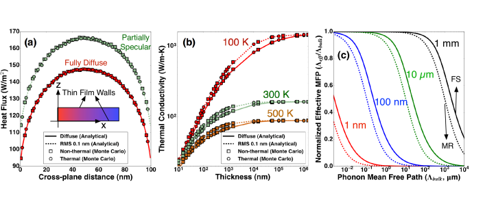
Figure 1: (a) Comparison of the cross-plane distribution of the in-plane steady state heat flux between analytical and Monte Carlo solutions of the BTE at 300 K and film thickness of 100 nm for different boundary conditions. The geometry of the thin film and the coordinate axes used in this work are shown in the inset. (b) Comparison of the steady state thermal conductivity between analytical and Monte Carlo solutions of the BTE at different temperatures and thin film thicknesses. For both (a) and (b), the Monte Carlo solutions are identical for thermalizing and non-thermalizing boundary scattering and agree well with the analytical solution derived in this work for both fully diffuse and partially specular boundary conditions (RMS 0.1 nm). For the partially specular boundary condition, the specularity parameter ($p_{\omega}$) is calculated from Ziman’s specularity model Ziman (1960) for a surface RMS roughness of 0.1 nm. (c) Effective MFPs of phonons computed using the Matthiessen’s rule (MR) and the Fuchs-Sondheimer (FS) theory for different film thicknesses and fully diffuse boundary scattering. Matthiessen’s rule underpredicts the effective phonon MFPs in thin films compared to the Fuchs-Sondheimer theory, which is a rigorous BTE solution.

III.1.2 Effective Phonon Mean Free Path

We also examine the effective mean free path (MFP) of phonons within the thin film for various film thicknesses. An approach to estimate the effective phonon mean free path in thin films is by using the Matthiessen’s rule Ziman (1960) given by,

$$\frac{1}{\Lambda_{\omega,\mathrm{eff}}}=\frac{1}{\Lambda_{\omega,\mathrm{bulk}}}+\frac{1-p_{\omega}}{1+p_{\omega}}\frac{1}{d}$$ (17)

where $d$ is the thickness of the thin film and $\Lambda_{\omega,\mathrm{bulk}}$ is the intrinsic phonon mean free path in the bulk material. Although the Matthiessen’s rule has been used in the past for computational  Dechaumphai and Chen (2012) and experimental Hochbaum et al. (2008) investigations of phonon boundary scattering, the mathematical rigor of such an expression for effective mean free path is unclear. On the other hand, the effective mean free path of phonons in thin films can also be determined rigorously from the Fuchs-Sondheimer factor ($F\left(\Lambda_{\omega}/d\right)$), since by definition, $F\left(\Lambda_{\omega}/d\right)=k_{\omega,\mathrm{eff}}/k_{\omega,\mathrm{bulk}}=\Lambda_{\omega,\mathrm{eff}}/\Lambda_{\omega,\mathrm{bulk}}$. Figure 1 (c) shows the comparison of the normalized effective phonon mean free paths obtained from the Fuchs-Sondheimer factor and Matthiessen’s rule for different film thicknesses. Matthiessen’s rule underpredicts phonon MFPs comparable to the thickness of the film. Even for phonons with intrinsic mean free path an order of magnitude smaller than the film thickness, Matthiessen’s rule predicts a shorter effective phonon mean free path compared to the predictions of the Fuchs-Sondheimer factor from the rigorous solution of the BTE, which is consistent with the findings of another work based on Monte Carlo sampling McGaughey and Jain (2012). This result highlights the importance of using the rigorous BTE solution to estimate the extent of diffuse phonon boundary scattering even in simple nanostructures.

III.2 Transient Transport in Thin Films

We now examine transient thermal conduction along thin films observed in the TG experiment. To perform this calculation, we solve the integral equation (equation 15) semi-analytically using the same isotropic phonon properties used in steady state transport calculations. The source term in the BTE (equation 10) is assumed to follow a thermal distribution given by $Q_{\omega}=C_{\omega}\Delta T_{0}$, where $C_{\omega}$ is the volumetric specific heat of the phonon mode.

III.2.1 Difference between Thermalizing and Non-thermalizing Boundary Scattering

Figure 2 (a) shows a comparison of the time traces calculated from the degenerate kernel method and the Monte Carlo method for a grating period of 20 $\mu$m. The transient decays are in good agreement between the degenerate kernel and the Monte Carlo solutions over a wide range of temperatures and different boundary conditions. As expected, the solution for the specular boundary condition results in a faster transient decay than the diffuse boundary conditions since a specularly reflecting wall does not resist the flow of heat in the in-plane direction. However, the transient decay for the non-thermalizing diffuse boundary condition is faster that the thermalizing diffuse boundary condition, indicating that the thermalizing boundary condition offers higher resistance to heat flow than the non-thermalizing diffuse scattering.

This observation is also evident from figure 2 (b) which shows the thermal conductivities obtained by fitting the time traces to an exponential decay for different temperatures, different grating periods and different boundary conditions. The observed thermal conductivity of the thin film decreases with decreasing grating period due to the breakdown of the Fourier’s law of heat conduction and the onset of quasiballistic thermal transport Hua and Minnich (2014b) when the grating period is comparable to phonon MFPs. Consistent with the findings from the time traces, the thermal conductivity of the thin film with specular walls is higher than that of the thin film with diffuse walls. Moreover, even for very long grating periods compared to phonon MFPs, where the thermal transport is diffusive and obeys Fourier’s law, the thermal conductivity of thin film with non-thermalizing diffuse walls is higher than that of the thin films with thermalizing diffuse walls. This observation is in stark contrast with the steady state condition, where there was no difference in thermal conductivity between thermalizing and non-thermalizing boundary conditions.

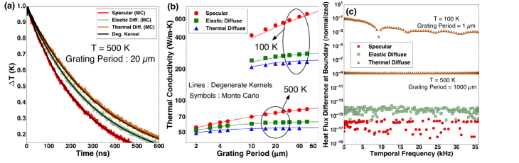
Figure 2: (a) Comparison between time traces from the Monte Carlo (colored noisy lines) and the degenerate kernels solutions (black lines) of the BTE for a grating period of $20\ \mu m$ at 500 K. (b) Comparison of the thermal conductivity predictions from the Monte Carlo (symbols) and the degenerate kernels solutions (black lines) of the BTE for different temperatures and grating periods. For both (a) and (b), the Monte Carlo solutions and the BTE solutions from this work are in very good agreement. (c) Plot showing the heat flux conservation at the film boundaries. Specular and non-thermalizing diffuse boundary conditions conserve heat flux to numerical precision while thermalizing diffuse boundary condition violates heat flux conservation at the film wall under quasiballistic (T = 100 K, grating period = $1\ \mu$m) and diffusive (T = 500 K, grating period = $1000\ \mu$m) transport regimes.

III.2.2 Validity of the Thermalizing and Non-thermalizing Boundary Conditions

At this point, it is important to investigate the validity of the thermalizing and non-thermalizing boundary condition for the thin film walls. The non-thermalizing boundary scattering condition can be naturally derived from the conservation of heat flux at the boundary Zeng and Chen (2000). However, the thermalizing boundary condition is not derived from the heat flux conservation at the boundary. Therefore, in the absence of any external scattering mechanisms, phonons cannot reach the local thermal equilibrium and simultaneously conserve heat flux at the boundary in general, due to the following reason.

Consider a boundary at $z=0$ separating a solid at $z>0$ from vacuum in $z<0$. The incoming phonon distribution at $z=0$ is $g^{-}_{\omega}\left(0,\mu,\phi\right)$, which is a general phonon distribution, not necessarily at the local thermal equilibrium. According to the formulation of the thermalizing diffuse boundary condition, the outgoing phonon distribution, in the case of fully diffuse boundary scattering, is given by $g_{0}\left(\Delta T\left(z=0\right)\right)\approx\frac{C_{\omega}}{4\pi}\Delta T\left(z=0\right)$, where $C_{\omega}$ is the heat capacity of the phonon mode and $\Delta T\left(z=0\right)$ is the local equilibrium temperature at the boundary $z=0$. Since the boundary separates a solid from vacuum, all of the heat flux incident on the boundary has to be reflected back into the solid. This constraint on the incident and reflected heat flux at the thermalizing diffuse boundary leads to the following relation for $\Delta T\left(z=0\right)$.

$$\Delta T\left(z=0\right)=4\frac{\sum_{p}\int_{\omega=0}^{\omega_{\mathrm{max}}}\int_{\mu=-1}^{0}\int_{\phi=0}^{2\pi}g^{-}_{\omega}\left(0,\mu,\phi\right)v_{g}\mu\mathrm{d}\mu\mathrm{d}\phi\mathrm{d}\omega}{\sum_{p}\int_{\omega=0}^{\omega_{\mathrm{max}}}C_{\omega}v_{g}\mathrm{d}\omega}$$ (18)

Additionally, energy conservation (equation 3) has to be satisfied at all locations including the boundaries in the absence of any other source or sink of phonons. This requirement further adds constraints on $\Delta T\left(z=0\right)$ through the relation,

$$\Delta T\left(z=0\right)=2\frac{\sum_{p}\int_{\omega=0}^{\omega_{\mathrm{max}}}\int_{\mu=-1}^{0}\int_{\phi=0}^{2\pi}\frac{g^{-}_{\omega}\left(0,\mu,\phi\right)}{\tau_{\omega}}\mathrm{d}\mu\mathrm{d}\phi\mathrm{d}\omega}{\sum_{p}\int_{\omega=0}^{\omega_{\mathrm{max}}}\frac{C_{\omega}}{\tau_{\omega}}\mathrm{d}\omega}$$ (19)

For the assumptions made in the Fuchs-Sondheimer theory under steady state transport conditions, the integrals of the incoming and the outgoing distribution functions (equation 7) over the azimuthal angle $\phi$ are $0$. Therefore, there is no heat flux towards or away from the boundary and the constraints on $\Delta T\left(z=0\right)$ (given by equations 18 and 19) are trivially satisfied. However, in general, these two expressions for $\Delta T\left(z=0\right)$ are not equal, indicating phonons cannot thermalize at the boundaries in the absence of any external source or sink of phonons.

Figure 2 (c) shows the difference between the incoming and outgoing total heat flux at the thin film wall ($z=0$) as a function of the temporal frequency $\eta$. The specular and non-thermalizing diffuse boundary conditions satisfy heat flux conservation to numerical precision. However, there is a significant difference between the incoming and the outgoing heat flux for the thermalizing diffuse boundary condition under quasiballistic (T = 100 K, grating period = $1\ \mu$m) and diffusive (T = 500 K, grating period = $1000\ \mu$m) transport regimes. Nevertheless, it is still possible for inelastic (but not thermalizing) diffuse boundary scattering to take place as long as the following conditions for heat flux are met at the thin film boundaries:

$$\begin{split}\sum_{p}\int_{\omega=0}^{\omega_{\mathrm{max}}}g^{+}_{\omega}\left(z=0\right)v_{g}\mathrm{d}\omega&=-\frac{1}{\pi}\sum_{p}\int_{\omega=0}^{\omega_{\mathrm{max}}}\int_{\mu=-1}^{0}\int_{\phi=0}^{2\pi}g^{-}_{\omega}\left(z=0,\mu,\phi\right)v_{g}\mu\mathrm{d}\mu\mathrm{d}\phi\mathrm{d}\omega\\ \sum_{p}\int_{\omega=0}^{\omega_{\mathrm{max}}}g^{-}_{\omega}\left(z=d\right)v_{g}\mathrm{d}\omega&=\frac{1}{\pi}\sum_{p}\int_{\omega=0}^{\omega_{\mathrm{max}}}\int_{\mu=0}^{1}\int_{\phi=0}^{2\pi}g^{+}_{\omega}\left(z=d,\mu,\phi\right)v_{g}\mu\mathrm{d}\mu\mathrm{d}\phi\mathrm{d}\omega\\ \end{split}$$

III.2.3 Comparison with Fuchs-Sondheimer Theory at Different Grating Periods

We now examine if the Fuchs-Sondheimer theory can be used to explain transient heat conduction in the TG experiment along thin films. If the suppression in thermal conductivity of thin films due to phonon boundary scattering and quasiballistic effects in the TG experiment are assumed to be independent, Fuchs-Sondheimer theory can be employed to describe quasiballistic transport in the TG experiment using the following expression:

$$k\left(q,d\right)=\sum_{p}\int_{0}^{\omega_{\mathrm{max}}}F\left(p_{\omega},\frac{\Lambda_{\omega}}{d}\right)S\left(q\Lambda_{\omega}\right)\left[\frac{1}{3}C_{\omega}v_{g}\Lambda_{\omega}\right]\mathrm{d}\omega$$ (20)

where $F\left(p_{\omega},\frac{\Lambda_{\omega}}{d}\right)$ is the Fuchs-Sondheimer suppression function from the steady state transport condition and $S\left(q\Lambda_{\omega}\right)$ is the quasiballistic suppression function Hua and Minnich (2014b) for a grating period $q$. Recent works Johnson et al. (2013) have used a similar expression for the thermal conductivity suppression of the form:

$$k\left(q,d\right)=\sum_{p}\int_{0}^{\omega_{\mathrm{max}}}F\left(p_{\omega},\frac{\Lambda_{\omega}}{d}\right)S\left(q\Lambda_{\omega}F\left(p_{\omega},\frac{\Lambda_{\omega}}{d}\right)\right)\left[\frac{1}{3}C_{\omega}v_{g}\Lambda_{\omega}\right]\mathrm{d}\omega$$ (21)

Henceforth, equation 20 is referred to as FS I and equation 21 is referred to as FS II. Figure 3 (a) shows the comparison of thermal conductivity obtained by fitting the BTE solution for temperature decay, and thermal conductivities from FS I and FS II models for fully diffuse boundary scattering. We only consider non-thermalizing diffuse scattering as we have shown that thermalizing diffuse scattering is unphysical for the problem considered here. At very long grating periods, when the transport is primarily diffusive, the thermal conductivity predictions from FS I and FS II match well with the BTE solution from this work, as expected. However, at the shorter grating periods comparable to phonon MFPs, where the transport is in the quasiballistic regime, FS I underpredicts the thin film thermal conductivity while FS II overpredicts it.

This observation is also evident from the magnitude of the suppression function plotted at $\eta=0$ for fully diffuse boundary conditions shown in figures 3 (b) and (c). The suppression function for the thin film geometry is defined as

$$S\left(q\Lambda_{\omega},\Lambda_{\omega}/d,\eta\tau_{\omega},p_{\omega}\right)=\frac{\kappa_{\omega,\mathrm{BTE}}}{\kappa_{\omega,\mathrm{Fourier}}}$$ (22)

where, $\kappa_{\omega}=j_{x,\omega}/\Delta\bar{T}$ is the conductance per phonon mode and $j_{x,\omega}$ is the thickness-averaged in-plane heat flux defined in equation 16. In figures 3 (b) and 3 (c), the magnitude of the suppression function at $\eta=0$ is plotted against phonon MFP non-dimensionalized with respect to the grating period $q$. The suppression functions from the complete BTE solution and the models FS I and FS II are identical at high temperatures and long grating periods, when the transport is primarily diffusive, governed by the Fourier’s law of heat conduction. However, for low temperatures and short grating periods, FS I underpredicts the heat flux and FS II overpredicts the heat flux carried by phonons with very long MFPs. Moreover, the difference between the models FS I and FS II, and the BTE solution is smaller for thinner films indicating that enhanced boundary scattering in thinner films delays the onset of quasiballistic heat conduction. These observations emphasize the importance of using the complete BTE solution to accurately investigate boundary scattering when grating periods are comparable to phonon MFPs.

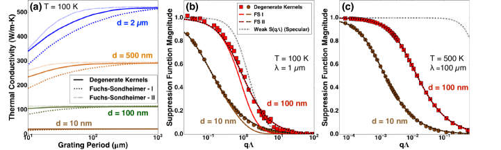
Figure 3: Comparison of the thermal conductivity (a) and the suppression functions ((b) and (c)) calculated from the models FS I, FS II and by solving the BTE for non-thermalizing diffuse boundary conditions at different temperatures, grating periods ($\lambda$) and film thicknesses. In figures (b) and (c), the symbols correspond to the degenerate kernel solution, the solid lines correspond to FS I model and the dashed solid lines correspond to FS II model. For very thin films and long grating periods, the models FS I and FS II are in good agreement with the BTE predictions. For thicker films and shorter grating periods, FS I underpredicts and FS II overpredicts the thermal conductivity at short grating periods (a) and the contribution of phonons with long MFP ((b) and (c)) compared to the complete BTE solution.

IV Conclusion

We have studied the effect of thermalizing and non-thermalizing boundary scattering of phonons in steady state and transient heat conduction along thin films by solving the BTE using analytical and computationally efficient semi-analytical techniques. From our analysis, we reach the following conclusions. First, under steady state transport conditions, we find that the thermal transport is governed by the Fuchs-Sondheimer theory and is insensitive to whether the boundaries are thermalizing or not. In contrast, under transient conditions, the decay rates are significantly different for thermalizing and non-thermalizing walls and the Fuchs-Sondheimer theory is only applicable in the heat diffusion regime. We also show that, for transient transport, the thermalizing wall boundary condition is unphysical due to violation of heat flux conservation. Our results provide insights into the boundary scattering process of thermal phonons over a wide range of heating length scales that are useful for interpreting thermal measurements on nanostructures.

V Acknowledgments

Navaneetha K. Ravichandran would like to thank the Resnick Sustainability Institute at Caltech and the Dow Chemical Company for fellowship support. Austin J. Minnich was supported by the National Science Foundation under Grant No. CBET CAREER 1254213.

References

- Cahill et al. (2014) D. G. Cahill, P. V. Braun, G. Chen, D. R. Clarke, S. Fan, K. E. Goodson, P. Keblinski, W. P. King, G. D. Mahan, A. Majumdar, H. J. Maris, S. R. Phillpot, E. Pop, and L. Shi, Applied Physics Reviews 1, 011305 (2014).
- Cho et al. (2014) J. Cho, Y. Li, W. E. Hoke, D. H. Altman, M. Asheghi, and K. E. Goodson, Physical Review B 89, 115301 (2014).
- Yan et al. (2012) Z. Yan, G. Liu, J. M. Khan, and A. A. Balandin, Nature Communications 3, 827 (2012).
- Koh et al. (2009) Y. K. Koh, Y. Cao, D. G. Cahill, and D. Jena, Advanced Functional Materials 19, 610 (2009).
- Poudel et al. (2008) B. Poudel, Q. Hao, Y. Ma, Y. Lan, A. Minnich, B. Yu, X. Yan, D. Wang, A. Muto, D. Vashaee, X. Chen, J. Liu, M. S. Dresselhaus, G. Chen, and Z. Ren, Science 320, 634 (2008).
- Biswas et al. (2012) K. Biswas, J. He, I. D. Blum, C.-I. Wu, T. P. Hogan, D. N. Seidman, V. P. Dravid, and M. G. Kanatzidis, Nature 489, 414 (2012).
- Fuchs (1938) K. Fuchs, Mathematical Proceedings of the Cambridge Philosophical Society 34, 100 (1938).
- Reuter and Sondheimer (1948) G. E. H. Reuter and E. H. Sondheimer, Proceedings of the Royal Society of London. Series A, Mathematical and Physical Sciences 195, pp. 336 (1948).
- Chen (2005) G. Chen, Nanoscale Energy Transport and Conversion - A Parallel Treatment of Electrons, Molecules, Phonons, and Photons (Oxford University Press, 2005).
- Cuffe et al. (2015) J. Cuffe, J. K. Eliason, A. A. Maznev, K. C. Collins, J. A. Johnson, A. Shchepetov, M. Prunnila, J. Ahopelto, C. M. Sotomayor Torres, G. Chen, and K. A. Nelson, Physical Review B 91, 245423 (2015).
- Turney et al. (2010) J. E. Turney, A. J. H. McGaughey, and C. H. Amon, Journal of Applied Physics 107, 024317 (2010).
- Casimir (1938) H. Casimir, Physica 5, 495 (1938).
- Aksamija and Knezevic (2010) Z. Aksamija and I. Knezevic, Physical Review B 82, 045319 (2010).
- Hao et al. (2009) Q. Hao, G. Chen, and M.-S. Jeng, Journal of Applied Physics 106, 114321 (2009).
- Mazumder and Majumdar (2001) S. Mazumder and A. Majumdar, Journal of Heat Transfer 123, 749 (2001).
- Ravichandran and Minnich (2014) N. K. Ravichandran and A. J. Minnich, Physical Review B 89, 205432 (2014).
- Li et al. (2003) D. Li, Y. Wu, P. Kim, L. Shi, P. Yang, and A. Majumdar, Applied Physics Letters 83, 2934 (2003).
- Hippalgaonkar et al. (2010) K. Hippalgaonkar, B. Huang, R. Chen, K. Sawyer, P. Ercius, and A. Majumdar, Nano Letters 10, 4341 (2010).
- Chen et al. (2008) R. Chen, A. I. Hochbaum, P. Murphy, J. Moore, P. Yang, and A. Majumdar, Physical Review Letters 101, 105501 (2008).
- Johnson et al. (2013) J. A. Johnson, A. A. Maznev, J. Cuffe, J. K. Eliason, A. J. Minnich, T. Kehoe, C. M. S. Torres, G. Chen, and K. A. Nelson, Physical Review Letters 110, 025901 (2013).
- Maznev et al. (2015) A. A. Maznev, F. Hofmann, J. Cuffe, J. K. Eliason, and K. A. Nelson, Ultrasonics 56, 116 (2015).
- Tang et al. (2010) J. Tang, H.-T. Wang, D. H. Lee, M. Fardy, Z. Huo, T. P. Russell, and P. Yang, Nano Letters 10, 4279 (2010).
- Minnich (2015) A. J. Minnich, Physical Review B 92, 085203 (2015).
- Hua and Minnich (2014a) C. Hua and A. J. Minnich, Physical Review B 90, 214306 (2014a).
- Hua and Minnich (2014b) C. Hua and A. J. Minnich, Physical Review B 89, 094302 (2014b).
- Hua and Minnich (2015) C. Hua and A. J. Minnich, Journal of Applied Physics 117, 175306 (2015).
- Zeng and Chen (2000) T. Zeng and G. Chen, Journal of Heat Transfer 123, 340 (2000).
- Peraud et al. (2014) J.-P. M. Peraud, C. D. Landon, and N. G. Hadjiconstantinou, Annual Review of Heat Transfer 17, 205 (2014).
- Liu and Asheghi (2004) W. Liu and M. Asheghi, Applied Physics Letters 84, 3819 (2004).
- Ju and Goodson (1999) Y. S. Ju and K. E. Goodson, Applied Physics Letters 74, 3005 (1999).
- Mingo et al. (2014) N. Mingo, D. Stewart, D. Broido, L. Lindsay, and W. Li, Length-Scale Dependent Phonon Interactions, edited by S. L. Shindé and G. P. Srivastava, Topics in Applied Physics, Vol. 128 (Springer New York, 2014) pp. 137–173.
- Li et al. (2012) W. Li, N. Mingo, L. Lindsay, D. A. Broido, D. A. Stewart, and N. A. Katcho, Physical Review B 85, 195436 (2012).
- Li et al. (2014) W. Li, J. Carrete, N. A. Katcho, and N. Mingo, Computer Physics Communications 185, 1747 (2014).
- (34) “A. Togo, Phonopy,” http://phonopy.sourceforge.net/.
- Kresse and Hafner (1993) G. Kresse and J. Hafner, Physical Review B 48, 13115 (1993).
- Kresse and Hafner (1994) G. Kresse and J. Hafner, Physical Review B 49, 14251 (1994).
- Kresse and Furthmüller (1996a) G. Kresse and J. Furthmüller, Computational Materials Science 6, 15 (1996a).
- Kresse and Furthmüller (1996b) G. Kresse and J. Furthmüller, Physical Review B 54, 11169 (1996b).
- Ziman (1960) J. M. Ziman, Electrons and Phonons. The theory of transport phenomena in solids (Oxford University Press, 1960).
- Dechaumphai and Chen (2012) E. Dechaumphai and R. Chen, Journal of Applied Physics 111, 073508 (2012).
- Hochbaum et al. (2008) A. I. Hochbaum, R. Chen, R. D. Delgado, W. Liang, E. C. Garnett, M. Najarian, A. Majumdar, and P. Yang, Nature 451, 163 (2008).
- McGaughey and Jain (2012) A. J. H. McGaughey and A. Jain, Applied Physics Letters 100, 061911 (2012).