Inversion of Tsunamis Characteristics from Sediment Deposits Based on Ensemble Kalman Filtering

Abstract

Sediment deposits are the only records of paleo tsunami events. Therefore, inverse modeling methods based on the information contained in the deposit are indispensable for deciphering the quantitative characteristics of the tsunamis, e.g., the flow speed and the flow depth. In this work, we propose an inversion scheme based on Ensemble Kalman Filtering (EnKF) to infer tsunami characteristics from sediment deposits. In contrast to traditional data assimilation methods using EnKF, a novelty of the current work is that we augment the system state to include both the physical variables (sediment fluxes) that are observable and the unknown parameters (flow speed and flow depth) to be inferred. Based on the rigorous Bayesian inference theory, the inversion scheme provides quantified uncertainties on the inferred quantities, which clearly distinguishes the present method with existing schemes for tsunami inversion. Two test cases with synthetic observation data are used to verify the proposed inversion scheme. Numerical results show that the tsunami characteristics inferred from the sediment deposit information agree with the synthetic truths very well, which clearly demonstrated the merits of the proposed tsunami inversion scheme. Furthermore, a realistic application of the proposed inversion scheme with the field data from the 2006 South Java Tsunami is studied, and the results are compared to the previous inversion model results in the literature and are validated with the field data. The comparisons show excellent performance of the proposed inversion scheme in realistic applications.

Gindraft=false WANG ET AL. ENKF-BASED TSUNAMI INVERSION Corresponding author: Heng Xiao, Department of Aerospace and Ocean Engineering, Virginia Tech, Blacksburg, VA 24060, USA. Email: hengxiao@vt.edu; Tel: +1 540 231 0926

Proposed a rigorous, Bayesian framework for tsunami inversion based on sediment deposits.

Used Ensemble Kalman filtering for inversion, providing quantified uncertainties in the results.

Verified and demonstrated inversion performance based on realistic setting of sediment deposits

1 Introduction

In recent decades, coastal cities have become important nodes in global economic network. Therefore, adverse impacts from coastal disasters, such as tsunamis, do not only have local or regional effects, but can amount to global consequences. Furthermore, the increased economic relevance of cities, such as Los Angeles, Singapore or Hong Kong (to mention only three of many), has caused their population to significantly grow, including projections that even more people will be attracted to these economic power houses. Because the population of coastal megacities increased and is predicted to grow even more, the risk from coastal disasters to which the coastal population is exposed needs to be carefully, realistically and objectively evaluated. To create risk assessments that meet these attributes, meaningful and robust hazard assessments are required. Fortunately for coastal megacites, not enough tsunamis have occurred in any one region to solely base hazard assessments on historical or modern record events. Because of that fact, the geologic record of paleo tsunamis needs to be interrogated. The important nature of the geologic record is the presence of uncertainty. This is not only because of the chaotic behavior of tsunami sources, such as earthquakes, landslide, volcanic eruptions, and meteorite impacts, but also due to the fact that, for example, storms can produce deposits with features similar to those preserved in tsunami deposits. There also are other sources of uncertainty. For example, the fact that the sedimentation process depends very strongly on the presence of local turbulence is an additional source of uncertainty that can only be reduced by a better understanding of sediment transport processes. The presence of uncertainty is one of the arguments employed to base tsunami hazard assessment on statistics.

To include the information contained in tsunami deposits, the often qualitative information retrieved from deposits needs to be translated into quantitative data about the causative event. Tsunami inversion models have been designed to estimate the flow conditions at the time of depositions. Models such as the Moore’s Advection Model  (Moore et al., 2007), Soulsby’s Model  (Soulsby et al., 2007) and TsuSedMod  (Jaffe and Gelfenbuam, 2007) were develop to retrieve quantitative data from the deposits about the causative event. While these models have been successfully applied (Moore et al., 2007; Soulsby et al., 2007; Jaffe and Gelfenbuam, 2007; Spiske et al., 2010; Jaffe et al., 2011, 2012; Witter et al., 2012; Spiske et al., 2013), the problem, however, is that these models cannot be seen as inversion models by a more strict definition of inversion. Specifically, important features of inversion models, such as uncertainty quantification and error analysis, cannot be properly carried out. To clarify, an inversion model performs an inversion based on a forward model and an inversion scheme. Without playing down the important impact the above-mentioned models have had, the present methods are more data-fitting models than inversion models in a strict, mathematical sense.

In this contribution, we propose a rigorous, Bayesian scheme for tsunami inversion based on Ensemble Kalman Filtering (EnKF). Data assimilation methods based on EnKF are widely used in geosciences applications such as numerical weather forecasting, where the initial conditions (present states of the system, e.g., pressure, velocity, and temperature) are not known precisely and thus must be inferred from observations. The novelty of the present work is the augmentation of the system state to include the unknown parameters and the use of EnKF-based data assimilation method to infer these parameters. To the authors’ knowledge, our work represents the first attempt to use EnKF for tsunami inversion. While this contribution should be seen as a proof of concept, a more comprehensive parameter study has been performed and will be presented in a separate paper. The proposed method would open up possibilities for mathematically more rigorous tsunami inversion from deposits with quantified uncertainties.

2 Methodology

The objective of this work is to infer tsunami flow characteristics from the tsunami deposits, which is an inverse problem. As with most inversion algorithm, the proposed method for the inverse problem involves solving the forward problem repeatedly, i.e., computing the tsunami deposit from given tsunami flow characteristics. Therefore, in this section the formulations, assumptions, and solution algorithm of the forward problem is first presented in Section 2.1. Subsequently, the formulation and solution algorithm for the inverse problem is introduced in Section 2.2.

2.1 Formulation of the Forward Problem and Solution Algorithm

Given the tsunami characteristics (i.e., flow speed $u$ and flow depth $h$), the forward problem is to compute the sediment deposition characteristics (i.e., the depth of the tsunami deposit and the particle size composition at any height of the sediment column). An example output of the forward problem is shown in Fig. 1c, which shows the thickness of the tsunami deposit, the grain-size distribution in each layer.

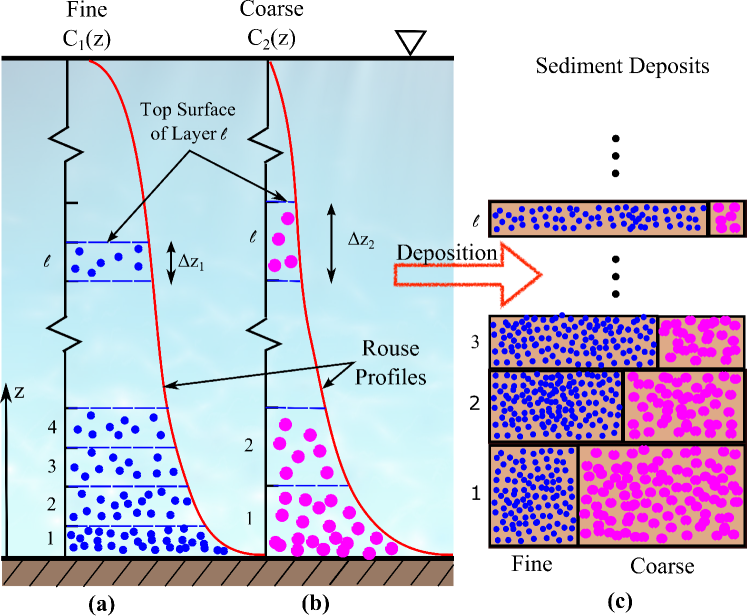
Figure 1: A schematic illustration of the algorithm for solving the forward problem, i.e., computing the tsunami deposit thickness and the grain-size distribution in each layer from given tsunami characteristics (flow speed and flow depth). An exemplary output of the algorithm is presented in Fig. 6.

The forward model adopted in this study is based on the simplified sedimentation models of Jaffe and Gelfenbuam (2007) and Tang and Weiss (2015). In these models it is assumed that the tsunami deposit is formed solely by the steady sedimentation of the particles in the water column. The effects of bed load transport and the acceleration of sediment particles during the settling process are neglected. It is further assumed that the sediment concentration and the fluid velocity vary only vertically in the water column, and their horizontal gradients and temporal changes are neglected. With the assumptions above, the flow velocity profile $u(z)$ along the water column can be parameterized by the shear velocity $u_{*}$, where $z$ is the elevation above the bed. Consequently, the depth-averaged flow velocity can be obtained from the following integral over the entire water column:

$$U=\int_{z_{0}}^{h}\frac{u_{*}^{2}}{K(z)}dz,$$ (1)

in which $z_{0}$ is the total roughness of the bed. The eddy viscosity $K$ can be calculated as following (Gelfenbaum and Smith, 1986):

$$K(z)=\kappa\,u_{*}\,z\exp\left[{\frac{-z}{h}-3.2\left(\frac{z}{h}\right)^{2}+\frac{2}{3}\times 3.2\left(\frac{z}{h}\right)^{3}}\right],$$ (2)

where $\kappa=0.41$ is the von Karman constant. The suspended sediment concentration for each grain size in the water column is assumed to follow the Rouse profile (Jaffe and Gelfenbuam, 2007):

$$C_{i}(z)=C_{i,0}\;\exp\left[{w_{i}\int_{z_{0}}^{z}{\frac{1}{K(z)}}}\right],$$ (3)

in which $w_{i}$ is the settling velocity of particles in the $i^{\mathrm{th}}$ grain-size class, which depends on the mean particle diameter $D_{i}$ of the class; $C_{i,0}$ denotes sediment concentration of the $i$^th grain-size class at the bed, which depends on the shear velocity $u_{*}$ and the fraction of bed sediment in class $i$, among other parameters (Madsen et al., 1993). Based on Eqs. (1) and (3), the velocity and concentration profiles can be uniquely parameterized by two scalar quantities, the shear velocity $u_{*}$ and flow depth $h$. Therefore, from here on we consider $u_{*}$ and $h$ the characteristics that define a tsunami. The objective of a tsunami inversion is thus to infer $u_{*}$ and $h$ from a tsunami deposit record.

Equation (3) suggests that the sediment concentration for each sediment grain size can be determined by the tsunami characteristics (i.e., shear velocity $u_{*}$ and flow depth $h$) and the particle diameter $D_{i}$. According to the convention in the sedimentology, the grain size is represented in $\phi$ scale (the logarithm of the particle diameter to the base 2), $\phi_{i}=-\log_{2}{(D_{i}/D_{\textrm{ref}})}$, in which $D_{\textrm{ref}}=1$ mm is the reference particle diameter to ensure dimensional consistency. Consequently, the tsunami deposit thickness and grain-size distribution can be obtained by integrating the concentration curve $C_{i}(z)$ for each grain size class. The integration is performed with the following algorithm, which is illustrated in Fig. 1 with two grain-size classes as an example.

1. Discretization of time. Assuming that $T$ is the total time taken for all the sediment in the water column (including all grain-size classes) to settle, we divide the time $T$ to $N$ time steps of size $\Delta t$ such that $T=N\,\Delta t$.

2. Discretization of water column. For grain-size class $i$, the water column can be divided to $N$ layers, numbered sequentially upward from the bottom (see Fig. 1a), such that the sediment at the top of layer $l$ arrives at the bed at time $l\,\Delta t$. Since the particles are assumed to have no acceleration (e.g., at constant velocity $w_{i}$) during the sedimentation, the layers of the water column have a uniform thickness of $\Delta z_{i}=w_{i}\,\Delta t$. Note that the layer thickness can be different among different grain-size classes since the terminal velocity $w_{i}$ is larger for coarse grains than for fine grains. Consequently, for a coarse grain-size class the discretized water column layer thickness $\Delta z_{i}=w_{i}\Delta t$ is larger and thus the number of discretized water column layers is smaller. This can be seen by comparing Fig. 1a and 1b.

3. Accumulation of tsunami deposit. With the discretization of the water column, it can be seen that the obtained tsunami deposit has $N$ layers as well (numbered in the same way as for the water column; see Fig. 1c). The sediment in layer $l$ consists of the sediment in the $l$^th layer of the water column for all grain-size classes (indicted in colors/patterns in Fig. 1c). The tsunami deposit thickness $\Delta\eta_{l}$ of the $l$^th layer is computed by summing up the sediment volume in the corresponding $l$^th water column layers for all grain-size classes:

   $$\Delta\eta_{l}=\frac{1}{C_{0}}\left(\sum_{i=1}^{n}{\overline{C}_{i,l}\,\Delta z_{i}}\right),$$ (4)

   in which $C_{0}$ is the total sediment concentration at the bed including size classes, $n$ is the number of grain-size classes, and $\overline{C}_{i,l}$ is the average concentration of grain-size class $i$ in the water column layer $l$, which can be obtained by a simple integration:

   $$\bar{C}_{i,l}=\frac{1}{\Delta z_{i}}\int_{z}^{z+\Delta z_{i}}\,C_{i}(z)\,dz.$$ (5)

4. Post-processing for grain-size distribution. The fraction $f_{i,l}$ of each grain-size class $i$ in the $l$^th layer in the sediment column is

   $$f_{i,l}=\frac{1}{C_{0}}\frac{\overline{C}_{i,l}\,\Delta z_{i,l}}{\Delta\eta_{l}}.$$ (6)

The thickness of sediment layers $\Delta\eta_{l}$ and the fraction $f_{i,l}$ for each grain-size class in each layer are used to produce the plots presented in Fig. 1c and Fig. 6, which is the final output of the forward problem.

The algorithm above for the forward problem produce some key information, which is the time stamp of tsunami deposit layers and the sediment flux at each time step. Specifically, the time at which the sediment layer $l$ finished the deposition at time $l\,\Delta t$, which can be considered the time stamp on the sediment layer (see Fig. 1b). Acknowledgedly, the sediment cores obtained in the field do not come with time stamps. However, by comparing sediment cores obtained at several locations with cross-shore offsets, it is possible to infer the time stamps and thus the sediment fluxes at discretized time intervals (Dearing et al., 1981).

To facilitate the filtering procedure to be used in the inversion, we adopt an alternative approach of computing tsunami deposit thickness by considering the time sequence of the sedimentation process. Specifically, in contrast to Eq. (4), the deposition thickness can be computed from the average sediment flux $\zeta_{i,l}$ of grain-size class $i$ at time step $l$ when the $l$^th layer of the sediment deposit is formed. That is,

$$\Delta\eta_{l} =\frac{1}{C_{0}}\left(\sum_{i=1}^{n}\zeta_{i,l}\,\Delta t\right),\quad\textrm{with}$$ (7a)

$$\begin{split}\zeta_{i,l}&=\frac{\overline{C}_{i,l}\,\Delta z_{i}}{\Delta t},\quad\textrm{or equivalently,}\\ \zeta_{i,l}&=\overline{C}_{i,l}\;w_{i}\quad\textrm{ in which }\quad w_{i}=\frac{\Delta z_{i}}{\Delta t}.\end{split}$$ (7b)

Note that the same subscript $l$ that is used above as the indices of the water column layer ( Fig. 1a and 1b) and sediment layer (Fig. 1c) is used to denote the time step index here. This choice of notation is justified by the assumption that the $l$^th sediment layer is formed by the deposition of all sediment grain classes in the $l$^th water column layer at time step $l$. Simply substituting Eq. (7b) to Eq. (7a) yields Eq. (4), and thus the two formulations in Eqs. (4) and (7) are equivalent.

By adopting the flux-based formulation, we are modeling the sediment deposition process as the evolution of a dynamical system with the sediment flux $\zeta_{i}$ for each grain-size class $i$ as the system state. Based on the assumptions from Eq. 7b, it can be seen that for any grain-size class $i$ the state $\zeta_{i}(t)$ is uniquely determined by the concentration profile $C_{i}(z)$ and the settling velocity $w_{i}$, which in turn depends on the tsunami characteristics (shear velocity $u_{*}$ and flow depth $h$) and the grain-size $\phi_{i}$. Therefore, the forward model $\mathcal{F}$ is thus formulated as to compute sediment deposition flux $\zeta_{i}(t)$ from known shear velocity $u_{*}$ and flow depth $h$, i.e., $\mathcal{F}:(u_{*},h)\mapsto\zeta_{i}(t)$. The sediment thickness and grain-size distribution are considered auxiliary quantities obtained by post-processing the time series of the system state $\zeta_{i}(t)$.

2.2 Formulation of the Inverse Problem and Solution Algorithm

The objective of the inverse problem is to infer the tsunami characteristics (depth-averaged flow velocity and flow depth) from tsunami deposit. In the formulation of the forward problem above, the flow velocity profile and the depth-averaged velocity are parameterized by the shear velocity as in Eq. (1), and the sediment flux is the state variable of the system. Therefore, the inverse problem is recast as inferring the shear velocity and flow depth from the sediment flux. The sediment flux, which is the input to the inverse problem, can be obtained by analyzing the tsunami deposit from the field. Specifically, when tsunami deposit samples are cored, they are first divided to a number of layers and to obtain the time stamp for each layer by utilizing the spatial information of the samples. Particle-size analysis is then performed on each layer, i.e., by using sieve analysis or other sedimentation techniques (Barth, 1984), which leads to the average sediment flux $\zeta_{i}$ at a few discrete time steps. The inverse problem needs to be formulated so that shear velocity $u_{*}$ and flow depth $h$ can be inferred from the sediment flux. As such, we consider $u_{*}$ and $h$ the unobservable parameters of the dynamical system $\mathcal{F}(u_{*},h;\zeta_{i}(t))$. They will be inferred from observations of the system state, i.e., the sediment flux $\zeta_{i}(t)$.

The inversion of shear velocity and flow depth from observed sediment flux is challenging for at least two reasons. First, the observation is inevitably sparse and noisy, because the sediment core can only be divided to a few layers to ensure each layer has enough sediment mass, and the measurement has large errors. Second, the forward model describing the sedimentation process is based on high simplified assumptions and thus does not faithfully represent the exact system dynamics.

In this work we use the Ensemble Kalman Filtering (EnKF) to perform the inversion (Evensen, 2003, 2009; Iglesias et al., 2013), which is widely used in data assimilations, particularly in numerical weather forecasting. When used to solve the tsunami deposit inversion problem, the system state is first augmented to include both the physical state $\zeta_{i}(t)$, which are observable, and parameters $u_{*}$ and $h$, which are unobservable (from the sediment core) and are to be inferred. The augmented system state $\mathbf{x}(t)$ is written as a vector formed by stacking the unknown parameters and the sediment flux $\zeta_{i}(t)$:

$$\mathbf{x}=[\zeta_{1},\cdots,\zeta_{n},u_{*},h]^{\prime},$$ (8)

in which ^′ indicates vector transpose.

Given the prior distributions for parameters ($u_{*}$ and $h$) to be inferred and the covariance matrix $\mathbf{R}$ of the sediment flux observations $\zeta_{i}^{obs}$, the inversion algorithm proceeds as follows:

1. Sampling of prior distribution. From the prior distributions of the parameters, $M$ samples are drawn. Each sample consists of a combination of values for $u_{*}$ and $h$.

2. Propagation. The sediment fluxes $\hat{\zeta}_{i}$ for all grain-size classes are computed from Eq. 7b by using the updated parameters $u_{*}$ and $h$ from the previous analysis step (or from the initial sampling if this is the first propagation step). The propagation is performed for $\Delta N$ time steps, where $\Delta N$ is the number of time steps in the time interval $\Delta T$ between two consecutive data assimilation operations. The $\hat{\cdot}$ indicates predicted quantities that will be corrected in the analysis step below. The propagation is performed for each sample in the ensemble, leading to the propagated ensemble $\{\hat{\mathbf{x}}_{j}\}_{j=1}^{M}$. Each sample $\hat{\mathbf{x}}_{j}$ is a vector containing a realization of shear velocity and flow depth as well as the corresponding sediment flux (see Eq. (8)). The mean $\bar{\mathbf{x}}$ and covariance $\mathbf{P}$ of the propagated ensemble are computed (see Eq. (10b) in Appendix A).

3. Analysis/Correction. The computed sediment fluxes $\hat{\zeta}_{i}$ for all grain-size classes are compared with observations $\zeta_{i}^{obs}$ corresponding to the current time step $l$. The ensemble covariance $\mathbf{P}$ and the error covariance $\mathbf{R}$ are used to compute the Kalman gain matrix $\mathbf{K}$. Each sample is corrected as follows:

   $$\mathbf{x}_{j}=\hat{\mathbf{x}}_{j}+\mathbf{K}({\boldsymbol{\zeta}_{j}}-\mathbf{H}\hat{\mathbf{x}}_{j})$$ (9)

   where superscript $\mathbf{x}_{j}$ is the corrected system state; $\boldsymbol{\zeta}=[\zeta_{1},\cdots,\zeta_{n}]^{\prime}$ are the sediment fluxes, the part of the system state vector that can be observed; $\mathbf{H}$ is the observation matrix. After the correction, the analyzed state contains updated fluxes and parameters.

   It should be remarked that: (1) the analysis scheme above suggest that the corrected state (i.e., the analysis) is a linear combination of the prediction and observations, with the Kalman gain matrix $\mathbf{K}$ being the weight of the observations; (2) the observation matrix $\mathbf{H}:\mathbb{R}^{n+2}\mapsto\mathbb{R}^{n}$ has a size of $n\times(n+2)$, which maps a vector in the $n+2$ dimensional state space to a vector in the $n$ dimensional observation space. The first $n$ columns of $\mathbf{H}$ are ones and the last two columns are zeros, indicating that the parameters are not observed.

4. Repeat propagation and analysis steps 2–3 for next data assimilation time $t+\Delta T$ to incorporate next observation until all observations are assimilated. The EnKF algorithm for inferring tsunami characteristics from tsunami deposit is summarized in Fig. 2. The detailed algorithm is presented in Appendix A.

It can be seen that the observations arrive sequentially in the EnKF data assimilation procedure above, which is typical for applications such as numerical weather forecasting. In this work we formulate the tsunami inversion problem with a sequential streaming of data to take advantage of the widely used EnKF algorithm. In this method, the filtering procedure finds an optimal correction at each assimilation step based on the latest observation and the latest prediction ensemble (see Eq. (9)). We note that it can be preferable to use another algorithm that is closely related to EnKF, namely the Ensemble Kalman Smoothing method, which finds optimal correction in light of all past observations (Evensen and Van Leeuwen, 2000). This method will be investigated in future work.

Figure 2: Schematic of the inverse modeling approach based on the state augmentation. The system state is augmented to include both the physical state (sediment flux $\zeta_{i}(t)$) and the parameters to be inferred (shear velocity $u_{*}$ and flow depth $h$). An ensemble representative of the augmented state is propagated via the forward model. The propagated ensemble is then updated in the analysis process based on the observation data. The updated state (physical quantities and model parameters) is then propagated to the next time step, and this loop continues until all observations are assimilated.

3 Computational Setup of Synthetic Cases for Verification

While EnKF-based Bayesian inferences have been widely used in other communities of geosciences, the present contribution represents the first attempt in using it for tsunami inversion. To establish confidence in the proposed framework for tsunami inversion based on sediment deposits, we construct a series of verification cases with synthetic truths to assess the performance of the proposed inversion scheme. Furthermore, we test the proposed framework by using a set of field data of the real tsunami deposits from the 2006 South Java Tsunami (sections Bunton, sample JTR 6 (Spiske et al., 2010)).

A synthetic case can be generated by running the forward model described in Section 2.1 on given a set of tsunami and sediment characteristics (i.e., shear velocity $\tilde{u}_{*}$ and flow depth $\tilde{h}$, the range of particle sizes $\tilde{\phi}_{i}$, where $\tilde{\cdot}$ indicates synthetic truths). The corresponding tsunami deposits including the thickness and the grain-size distribution as shown in Fig. 6 can thus be obtained. Subsequently, the sediment flux can be obtained by post-processing the tsunami deposit information with the procedure explained in Section 2.2. In fact, for the synthetic cases the sediment fluxes are part of the forward model simulation output, and thus a post-processing procedure is not required. Synthetic observations are then generated by adding Gaussian random noises of standard deviation $\sigma_{i}$ to the true sediment fluxes, which represent the measurement and sampling errors in sediment coring operations in the field. The decision to use synthetic cases instead of realistic cases to verify the proposed method is justified by the fact that the true tsunami characteristics corresponding to actual field samples are usually unknown, which make them not ideal for verification purposes. Even if the truth for tsunami characteristics were known, e.g., when the flow speed and flow depth were measured from independent sources, it would be difficult to distinguish the errors due to the forward model inadequacy and those due to the inversion procedure. Therefore, using the synthetic cases allow us to focus on assessing the performance of the proposed inversion procedure. The merits of the inversion scheme can be assessed by its capability to reproduce the synthetic truths $\tilde{u}_{*}$ and $\tilde{h}$, to which the inversion scheme is blind. With the established confidence from the verification cases, field data of deposits from the 2006 Java tsunami event are used as the observations to demonstrate the capability of the proposed framework in realistic applications.

For simplicity, we assume that the shear velocity $u_{*}$ and flow depth $h$, which are to be inferred, are assumed time-invariant. In addition, tsunami deposit at only one onshore location is utilized. The proposed scheme can be straightforwardly extended to time-varying shear velocity $u_{*}(t)$ by incorporating iterations in each time step. Moreover, for the problems where sediment deposits are available at multiple locations, the proposed scheme also can be applied by expanding the state vector to include fluxes at different locations.

Two verification cases with synthetic observations of increasing difficulty levels are defined. In case 1, the sediment has a single grain size $\phi=2.0$, and the only unknown parameter to be inferred is the shear velocity $u_{*}$ while the flow depth $h$ is given. In case 2, which is more challenging, the sediment has a log-normal grain-size distribution with $0<\phi<3.25$. Both $u_{*}$ and $h$ are unknown and are to be inferred. The synthetic truths for $u_{*}$ and $h$, the prior ensemble means ($\bar{u}_{*}^{0}$ for both cases and $\bar{h}^{0}$ for case 2 only) are the same for both synthetic cases. For the realistic case with field data (referred to as case 3), the mean grain size, largest grain size and smallest grain size are $\phi=2.5$, $\phi=0.0$ and $\phi=5.25$, respectively. The mean values of prior ensembles are estimated by TSUFLIND (Tang and Weiss, 2015). All other parameters, including the forward model time step $\Delta t$, the data assimilation interval $\Delta N$, and the number of samples $M$ are the same for all 3 cases. The parameters are summarized in Table 1. The prior ensembles for both parameters are uniformly distributed in the ranges specified in Table 1, which is representative of the lack of knowledge on the quantities to be inferred in practical tsunami inversions. Since the truths of the quantities to be inferred, $\tilde{u}_{*}$ and $\tilde{h}$, are unknown when performing the inversion, the mean values of prior ensemble $\bar{u}_{*}^{0}$ and $\bar{h}^{0}$ for both quantities are likely to have biases compared to the synthetic truth. This is reflected in the choice of ensemble mean as shown in Table 1. The time step $\Delta t=0.5$ s is chosen for all cases, and the observations of sediment fluxes are assimilated every $\Delta N=10$ time steps. The error covariance matrix is chosen as $\mathbf{R}=\textrm{diag}[\sigma_{1}^{2},\cdots,\sigma_{n}^{2}]$ with $\sigma_{i}$ being the standard deviation of the white noise added to the true sediment fluxes for each grain size $i$. The choice of standard deviation of noises shown in Table 1 is based on the error model detailed in a companion paper.

Table 1: Physical and computational parameters for test cases.

Parameters	Case 1	Case 2	Case 3
Inferred parameters	$u_{*}$	$u_{*}$ and $h$	$u_{*}$ and $h$
Grain size $\phi$ $(=-\log_{2}[D/D_{\textrm{ref}}])$	$2.0$	$0<\phi<3.25$	$0<\phi<5.25$
$\Delta t$	0.5 s
Data assimilation interval $\Delta N$	10
Number of samples $M$	1000
std. $\sigma_{i}$ of observation errora	$\epsilon$ + 0.01$\tilde{\zeta}_{i}$		$\epsilon$ + 0.05$\tilde{\zeta}_{i}$
Synthetic truth $\tilde{u}_{*}$ for $u_{*}$	$0.5\ \mathrm{ms}^{-1}$		$-$
Range of prior ensemble for $u_{*}$ b	0.4 to $1.2\ \mathrm{ms}^{-1}$		0.15 to $0.45\ \mathrm{ms}^{-1}$
Mean $\bar{u}_{*}^{0}$ of prior ensemble for $u_{*}$	$0.8\ \mathrm{ms}^{-1}$		$0.3\ \mathrm{ms}^{-1}$
Synthetic truth $\tilde{h}$ for $h$	3 m	3 m	$-$
Range of prior ensemble for $h$	$-$	2.5 to 7.5 m	6 to 10 m
Mean $\bar{h}^{0}$ of prior ensemble for $h$	$-$	5 m	8 m

a std. denotes standard deviation; the standard deviation of noise added to the observation depend on the grain-size class; $\epsilon=0.125$ $\mathrm{mm^{3}s^{-1}}$ is a fixed constant, and $\tilde{\zeta}$ is the synthetic truth of the sediment flux, which depends on the grain size and vary with time bA smaller range of prior ensemble for $u_{*}$ from 0.7 to 0.9 $\mathrm{ms^{-1}}$ is also investigated in case 1.

4 Results and Discussion

4.1 Case 1: A Single Grain-Size Class and One Unknown Parameter

First, a case with simple conditions is studied where all tsunami deposits are in the same grain-size class and the shear velocity $u_{*}$ is the only unknown parameter to be inferred. Although this highly simplified scenario is likely to be uncommon in reality, a case with controlled conditions is able to provide a reasonable initial assessment of the proposed method.

The time series $\zeta(t)$ of the sediment flux, which is the physical state of the system, is presented in Fig. 3. The sediment fluxes for all 1000 samples are shown along with the synthetic truth corresponding to the true shear velocity $\tilde{u}_{*}=0.5\ \mathrm{ms}^{-1}$. It can be seen that for all samples (i.e., prior guesses of shear velocities) and the synthetic truth show a general trend that the magnitude of sediment flux decreases with time, which is typical for a Rouse sediment concentration profile assumed in the forward model as in Eq. (3).

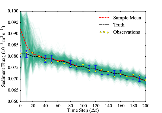
Figure 3: Time series of the sediment fluxes $\zeta(t)$, which is the physical state of the system, for a single grain-size class $\phi=2.0$ during the sedimentation process. The green (light grey) lines show $M=1000$ sediment flux samples, and the yellow (filled) circles indicate the observed sediment flux corresponding to the synthetic truth of the shear velocity $\tilde{u}_{*}=0.5\ \mathrm{ms}^{-1}$. (The 2$\sigma_{o}$ observation error bar is also plotted in the figure.) The synthetic observation data of sediment fluxes are assimilated to the simulation every 10 times in the EnKF-based inversion procedure.

s

The convergence history of the inferred parameter, the shear velocity $u_{*}$, is shown in Fig. 4a. By assimilating the observation data as shown in Fig. 3, the shear velocity of all samples and the sample mean gradually converge to the synthetic truth $\tilde{u}_{*}=0.5\ \mathrm{ms}^{-1}$, regardless of their values in the initial ensemble. The range of sample scattering for $u_{*}$, which is $0.8\ \mathrm{ms}^{-1}$ (with a range from 0.4 to $1.2\ \mathrm{ms}^{-1}$) in the prior ensemble, shrinks to $0.04\ \mathrm{ms}^{-1}$ at the end of the inference. Since the scattering of samples in EnKF-based inference is indicative of the uncertainty in the inferred results, the reduction of sample scattering represents the reduction of uncertainties and correspondingly the increase of confidence in the quantity to be inferred.

The Probability Density Function (PDF) of the shear velocity $u_{*}$ corresponding to the ensemble at time steps 0 (initial), 30, 50, 100 and 200 (final) are presented in Fig. 4b, highlighting the evolution of uncertainty in the inferred quantity. We can see that the shear velocity $u_{*}$ is equally likely between 0.4 and $1.2\ \mathrm{ms}^{-1}$ because of the non-informative, uniform prior distribution that is chosen. At time step 50 (after five observations assimilated) the samples are scattered between approximately 0.47 and $0.54\ \mathrm{ms}^{-1}$. Moreover, the bias of the ensemble mean compared to the truth has been largely corrected. As the data assimilation continues, the distribution of $u_{*}$ continues to shrink and concentrate towards the truth ($\tilde{u}_{*}=0.5\ \mathrm{ms}^{-1}$). The final, posterior distribution of $u_{*}$ at time step 200 is Gaussian based on the plot shown in Fig. 4b. While this could well be the true distribution, it should be interpreted with caution, since it is well known that the EnKF procedure tend to give a Gaussian distribution because of its assumptions Evensen (2009). The Cumulative Distribution Function (CDF) of the posterior distribution is presented in Fig. 4c. It shows that 95% of ensembles have shear velocities $u_{*}$ between 0.490 and 0.508 $\mathrm{ms}^{-1}$. In other words, the inference suggest that there is 95% probability that the shear velocity $u_{*}$ falls within the range above. This credible interval is based on both the prior distribution and the observation data.

The uncertainties represented as credible intervals that are obtained in the inversion process is based on the rigorous Bayesian inference theory, which clearly distinguishes the present method with existing schemes for tsunami inversion. The evolution of the inference uncertainty over time as shown in Fig. 4a and 4b illustrates the Bayesian nature of the EnKF-based data assimilation method. In the inference, one starts with a subjective prior distribution on the unknown parameters, which is usually non-informative (see the wide distribution at time step 0) and is represented with an ensemble. As observation data are assimilated, the distribution becomes narrower. Meanwhile, the importance of the prior distribution diminishes as more and more data are assimilated. The remaining uncertainties in the inference results stems from the uncertainties in the observation data, which are inevitable in field measurement and are represented with random noise in this study.

In order to demonstrate the robustness of the inversion procedure with respect to the specified prior distribution, we also tested a prior ensemble (i.e., initial guesses of the parameter to be inferred) with $u_{*}$ in the range of 0.7 and $0.9\ \mathrm{ms}^{-1}$. In contrast to the case presented above, this range does not cover the truth $\tilde{u}_{*}=0.5\ \mathrm{ms}^{-1}$. Even with this overly confident prior distribution, almost identical inversion results were obtained. In fact, the differences between the convergence history of $u_{*}$ disappear after a few assimilation steps. As such, detailed results for this case are omitted here for brevity.

The relative inference error for the shear velocity is presented in Fig. 5, which is defined as the $L_{2}$ norm $|(\bar{u}_{*}-\tilde{u}_{*})/\tilde{u}_{*}|$ of the difference between the ensemble mean $\bar{u}_{*}$ and the synthetic truth $\tilde{u}_{*}$. It can be seen that the inference error decreases dramatically within the first few data assimilations steps, from $0.6$ for the initial prior ensemble (time step 0) to $0.025$ after five observations are assimilated (at time step 50). This finding is consistent with the decrease of the ensemble scattering (indicating inference uncertainties) as shown in Fig. 4a.

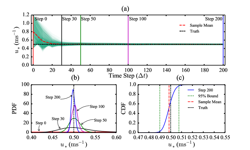
Figure 4: Convergence history of the inferred parameter, the shear velocity $u_{*}$, for the single grain-size case. The plot shows (a) the convergence of the ensemble and the sample mean as well as (b) the evolution of the probability density function of the shear velocity $u_{*}$ in the inversion process. (c) The corresponding cumulative distribution function for the final inference results.

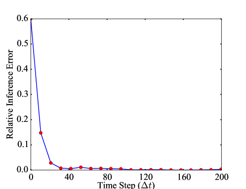
Figure 5: The $L_{2}$ norm of the inference error for the shear velocity, defined as the difference $|(\bar{u}_{*}-\tilde{u}_{*})/\tilde{u}_{*}|$ between the ensemble mean $\bar{u}_{*}$ and the synthetic truth $\tilde{u}_{*}$.

4.2 Case 2: Multiple Grain-Size Classes and Two Unknown Parameters

A tsunami inversion problem with wide grain-size distribution is studied to demonstrate the capability of the proposed method in a more realistic scenario. Both the shear velocity $u_{*}$ and the flow depth $h$ are unknown and the two parameters must be inferred simultaneously. The input to the tsunami inversion procedure is the analyzed results of tsunami deposit column as shown in Fig. 6. The grain-size distribution along the depth of the sediment column is obtained from a forward simulation with shear velocity and flow depth as specified in Table 1. The particle sizes range from 0 to 3.25 in $\phi$ scale, or equivalently from 1 mm to 0.105 mm. The range is divided into 10 grain-size classes, $\phi_{i}$ with $i=1,\cdots,10$, equally spaced in $\phi$ scale. The superscripts are indices of the grain-size classes.

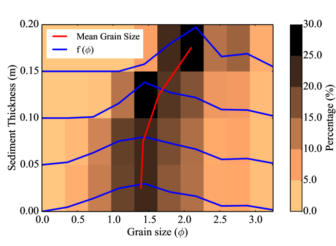
Figure 6: Hypothetical 0.2 m thick tsunami deposit for verification cases: vertical grading in grain-size distributions (blue line) and mean grain-size (red line) for sediment intervals. The grain-size distribution of the entire tsunami deposit is a log-norm distribution.

The time series of sediment fluxes for six representative grain-size classes are shown in Fig. 7, i.e., $\phi_{2}=0.65$, $\phi_{3}=0.975$, $\phi_{4}=1.3$, $\phi_{5}=1.625$, $\phi_{6}=1.95$, and $\phi_{7}=2.275$. As in the case with a single grain-size class, the sediment fluxes $\zeta_{i}(t)$ for all grain-size classes decrease as the deposition proceeds, and the uncertainties represented by the ensemble scattering are reduced as the observations are assimilated. Moreover, the sediment fluxes for the coarse grains (corresponding to smaller $\phi$ values, e.g., $\phi_{2}=0.65$, $D=0.637$ mm as shown in Fig. 7a) decrease more rapidly than those for the finer grains with larger $\phi$ values. It can be seen from Fig. 7a that the coarsest ($\phi_{2}=0.65$) among the six grain-size classes completed sedimentation in 60 time steps (i.e., 30 seconds since $\Delta t=0.5$ s). In contrast, the finest grain-size class ($\phi_{7}=2.275$, $D=0.105$ mm) among the six has a more uniform sediment flux throughout the entire sedimentation process. Again, this is attributed to the assumed Rouse profile. It is also noted that the relative uncertainties (ensemble scattering) in the sediment fluxes at the end of the inversion are larger for the fine grains than for the coarse grains. This is due to the random noises added to the true sediment flux when generating synthetic observations. As shown in Table 1, the standard deviation $\sigma_{i}$ of the noise has a fixed component ($\epsilon$) and a component $0.01\tilde{\eta}_{i}$ proportional to the truth. Since the sediment flux for the finer grains are smaller in absolute value, as can be seen from the different vertical axis ranges in panels (a)–(f), the relative observation uncertainties are thus larger for the sediment fluxes of the finer grain sizes. Consequently, the uncertainties in ensemble directly reflect the uncertainties in the observations.

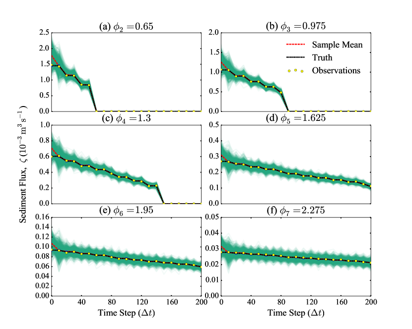
Figure 7: Time series of sediment fluxes $\zeta(t)$ for six (among a total of 10) grain-size classes during the sedimentation: (a) $\phi_{2}=0.65$, (b) $\phi_{3}=0.975$, (c) $\phi_{4}=1.3$, (d) $\phi_{5}=1.625$, (e) $\phi_{6}=1.95$, and (f) $\phi_{7}=2.275$. The green (light grey) lines show $M=1000$ samples of sediment flux time series, and the yellow (filled) circles indicate the observed sediment flux corresponding to the synthetic truth, i.e., shear velocity $\tilde{u}_{*}=0.5\ \mathrm{ms}^{-1}$ and flow depth $h=3$ m. synthetic observation data of sediment fluxes are assimilated to the simulation every 10 times in the EnKF-based inversion procedure.

The convergence history of the two parameters to be inferred, shear velocity and flow depth, are presented in Fig. 8. It can be seen from Fig. 8a and 8b that the sample means for both parameters (red dotted lines) converge to the synthetic truths (horizontal black dashed lines) within 50 time steps, i.e., after five observations are assimilated, although the prior ensemble means deviate significantly from the truths at time step 0. Moreover, the uncertainties as indicated by the ensemble scattering are reduced significantly. We note two points here. First, comparison between Fig. 8a and 8b suggests that the shear velocity converges to the truth faster than the flow depth does. Since EnKF inversion procedure depends on correlation to make inferences, this seems to indicate that the sediment fluxes, which are the observed physical state, are more sensitive to the shear velocity than that to the flow depth. Second, the convergence of shear velocity in the multiple grain-size case as shown in Fig. 8b is slightly faster than that in the single grain-size class case in Fig. 4a. A major difference between the two cases is that the state in the multiple grain-size case is the sediment flux for all grain-size classes, i.e., a vector of size 10 with one component corresponding to each grain-size class. Accordingly, an observation in the multiple grain-size case is also a vector of size 10. This is much more information than in the single grain-size class case, where the state and observations are only scalars. More information in the observation leads to more accurate inference. Intuitively, one would expect the multiple grain-size class case to be more difficult, particularly considering the fact that there are two unknown parameters. Indeed, this apparently counterintuitive finding suggests that the setup here is not entirely realistic in that we used similar levels of relative error for both the single and multiple grain-size cases. In the field, when a sediment core of a given size is divided to yield grain-size distributions for multiple grain-size classes, the relative measurement error in the obtained grain-size distribution would inevitably increase compared to a single grain-size class case. Therefore, it would have been more realistic to use a larger observation error for the multiple grain-size case. The effect of observation errors on the inference results and the optimization of number of grain-size classes from a given sediment core are topics of future work. The decrease of uncertainties in the inferred parameters can be clearly seen in the probability density functions shown in Fig. 8c and  8d. For both parameters, the probability density functions shrink continuously towards the truth, indicating the gain of confidence as more observations are assimilated. Overall, in this more realistic and challenging test case, we found that the proposed method has equally satisfactory performance compared to that in the single grain-size case.

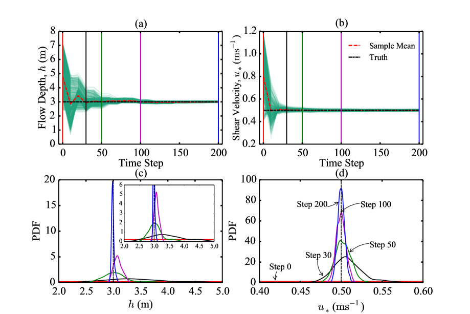
Figure 8: Convergence history of the inferred parameters, the shear velocity $u_{*}$ and the flow depth $h$. Panels (a) and (b) show the evolution of the ensemble and the sample mean for the shear velocity and the flow depth, respectively. Panels (c) and (d) show the evolution of probability density functions for the shear velocity and the flow depth, respectively, during the inversion process. In panel (c) a zoomed-in view is presented as inset to show the detailed results in the first few steps.

4.3 Case 3: Realistic Application

For this case, a deposit column with a 0.12 m thickness from the 2006 South Java Tsunami is used as the observation. We simultaneously infer both unknown parameters, shear velocity $u_{*}$ and flow depth $h$. The particle sizes range from 0 to 5.25 in $\phi$ scale, or equivalently from 1 mm to 0.0263 mm in diameter. We divided this range into 15 grain-size classes $\phi_{i}$ with $i=1,\cdots,15$, equally spaced in $\phi$ scale.

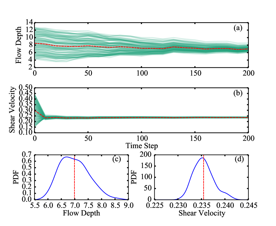
Figure 9: Convergence history of the inferred parameters, the shear velocity $u_{*}$ and the flow depth $h$, for case 3. Panels (a) and (b) show the evolution of the ensemble and the sample mean for the shear velocity and the flow depth, respectively. The green (light grey) lines denote samples and the red dashed lines denote sample means. Panels (c) and (d) show the probability density functions for the inferred shear velocity and the flow depth, respectively, at the final time step (200). The sample mean is denoted with red dashed line.

The convergence history of shear velocity and flow depth is presented in Fig. 9. We can see that the scattering of both parameters is reduced. Within 200 steps, flow depths in most of the samples converges to the range of 6 to 8 m from initial range of 4 to 12 m. Meanwhile, shear velocities in the samples converges to a small interval around 0.235 $\mathrm{ms^{-1}}$. Similar to what has been shown in synthetic case 2, the shear velocity converges faster than the flow depth does. The scattering of shear velocity samples is significantly reduced after 200 steps, while the flow depth samples are still largely scattered, indicating a relatively large posterior inference uncertainty. This is because the sediment fluxes are not sensitive to the flow depth, especially when the flow depth is large. Specifically, the Rouse profiles depicted in Fig. 1 shows that the sediment concentration is low in the upper region of the water column. When the flow is deep, the change of its depth does not significantly affects the sediment concentration in the upper layers of the water, and thus the sediment fluxes are not sensitive to the flow depth. The probability density functions of the flow depth and shear velocity in the last time step (posterior) are shown in Fig. 9c and 9d, respectively. The posterior distributions of flow depth and shear velocity are approximately Gaussian with mean values of 7.0 m and 0.236 ms^-1, respectively.

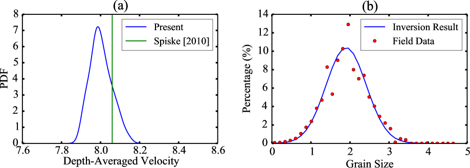
Figure 10: Comparison of two inferred QoIs, the depth-averaged velocity and the grain-size distribution, with the previous inference of  (Spiske et al., 2010) (depth-averaged velocity) and field data (grain-size distribution), respectively. Panel (a) shows the comparison of depth-averaged velocity calculated based on the inferred shear velocity $u_{*}$ and water depth $h$ from the proposed inversion scheme with that of TsuSedMod results (Spiske et al., 2010). Panel (b) compares the grain-size distribution obtained from the forward simulation with the inferred parameter $u_{*}$ and $h$ with the field data.

Since there are no ground truths of flow depth and shear velocity available for validation in this realistic case, we have to validate the inference results indirectly. Specifically, the depth-averaged velocity is computed by using the inferred shear velocity and flow depth based on Eq. 1 and is compared with that obtained by Spiske et al. (2010) with the inversion model TsuSedMod. The comparison is shown in Fig. 10a. We can see that the depth-averaged velocity from our inference is distributed from 7.8 to 8.2 ms^-1 with a mean value of 8.0 ms^-1. This posterior credible interval covers the inference result (8.06 ms^-1) of Spiske et al. (2010), although the sample mean from our inference is slightly smaller. A possible explanation of the discrepancy is that Spiske et al. (2010) used the entire deposit for the TsuSedMod model to perform the inversion, but the sediments in the bottom layers of the deposit may be transported by bed load. Since the TsuSedMod model assumes the sediments is formed only by suspension load (Jaffe and Gelfenbuam, 2007), the velocity obtained by Spiske et al. (2010) may have been overestimated. In order to compare the inversion results with the field data, we perform forward simulations of sedimentation with the inferred parameters, i.e., mean values of posterior flow depth and shear velocity. Figure 10b compares the grain-size distribution obtained based on the inferred parameters with that from the field data. It can be seen that the inferred grain-size distribution agrees very well with the field data, which shows a satisfactory performance of the proposed inversion scheme in the realistic case. However, it should be noted that this indirect validation of the inference does not guarantee the inferred quantities (i.e., flow depth and shear velocity) are accurate, since the model error of the forward model affects the accuracy of the inversion. If the forward model adequately describes the physics of the sedimentation process, the inference results are accurate. Therefore, we can improve the forward model to achieve more accurate inference results.

5 Conclusion

In this work, we proposed a novel inversion scheme based on Ensemble Kalman Filtering to infer tsunami flow speed and flow depth from tsunami deposits. In contrast to traditional data assimilation methods using EnKF, an important novelty of the current work is that the system state is augmented to include both the physical variables (sediment fluxes) and the unknown parameters to be inferred, i.e., shear velocity and flow depth. Consequently, the unknown tsunami characteristics are inferred in a rigorous Bayesian way with quantified uncertainties, which clearly distinguishes our method with existing tsunami inversion schemes. Two test cases with synthetic observation data are used to verify the proposed inversion scheme. Numerical results show that the tsunami characteristics inferred from the tsunami deposit information have favorable agreement with the synthetic truths, which demonstrated the merits of the proposed tsunami inversion scheme. A realistic case with field data is studied, and the results are compared to those obtained with a previous inversion model TsuSedMod and are validated by the field data. The comparisons indicate a satisfactory performance of the proposed inversion scheme on realistic applications. The proposed inversion scheme is a promising tool for the study of paleo tsunamis in the interrogation of sediment records to infer tsunami characteristics.

Appendix A Detailed Algorithm for Ensemble Kalman Filtering

The algorithm of the ensemble Kalman filtering for data assimilation and inverse modeling is summarized below.

Given the prior distribution of the parameters to be inferred (shear velocity $u_{*}$ and flow depth $h$) and sediment flux observations with error covariance matrix $\mathbf{R}$, the following steps are performed:

1. (Sampling step) Generate initial ensemble $\{{\mathbf{x}_{j}}\}_{j=1}^{M}$ of size $M$, where the augmented system state is:

   $$\mathbf{x}=[\zeta_{1},\cdots,\zeta_{n},u_{*},h]^{\prime}.$$

2. (Prediction step)

   1. Propagate the state from current state at time $t$ to the next assimilation step $t+\Delta T$ with the forward model TSUFLIND, indicated as $\mathcal{F}$,

      $$\hat{\mathbf{x}}_{j}^{(t+\Delta T)}=\mathcal{F}[\mathbf{x}_{j}^{(t)}]$$

      in which $\Delta T=\Delta N\Delta t$, indicating that the observation data is assimilated every $\Delta N$ time steps.

   2. Estimate the mean $\bar{\mathbf{x}}$ and covariance $\mathbf{P}^{(n+1)}$ of the ensemble as:

      $$\bar{\mathbf{x}}^{(t+\Delta T)}=\frac{1}{M}\sum_{j=1}^{N}{\hat{\mathbf{x}}^{(t+\Delta T)}_{j}}$$ (10a)

      $$\mathbf{P}^{(t+\Delta T)}=\frac{1}{M-1}\sum_{j=1}^{N}{\left(\hat{\mathbf{x}}_{j}\hat{\mathbf{x}}_{j}^{\prime}-\bar{\mathbf{x}}\bar{\mathbf{x}}^{\prime}\right)^{(t+\Delta T)}}$$ (10b)

3. (Analysis step)

   1. Compute the Kalman gain matrix as:

      $$\mathbf{K}^{(t+\Delta T)}=\mathbf{P}^{(t+\Delta T)}\mathbf{H}^{\prime}(\mathbf{H}\mathbf{P}^{(t+\Delta T)}\mathbf{H}^{\prime}+\mathbf{R})^{-1}$$

   2. Update each sample in the predicted ensemble as follows:

      $$\mathbf{x}_{j}^{(t+\Delta T)}=\hat{\mathbf{x}}_{j}^{(t+\Delta T)}+\mathbf{K}(\boldsymbol{\zeta}_{j}-\mathbf{H}\hat{\mathbf{x}}_{j}^{(t+\Delta T)})$$

4. Repeat the prediction and analysis steps until all observations are assimilated.

Appendix B Notation

$h$	water depth
$n$	number of grain-size classes
$U$	depth-averaged flow speed
$u_{*}$	shear velocity
$w$	settling velocity of particles
$z$	elevation above the bed
$z_{0}$	total roughness of the bed
$\mathbf{x}$	augmented system state
$C(z)$	vertical profile of sediment concentration
$C_{i,0}$	sediment concentration of class $i$ at the bed
$C_{0}$	total sediment concentration at the bed
$D$	mean particle diameter
$\mathcal{F}$	forward model for sedimentation
$K$	eddy viscosity
$M$	number of samples
$N$	number of time steps
$T$	total time for all sediments to settle
$U$	depth-averaged flow velocity
$\mathbf{R}$	observation covariance matrix
$\mathbb{R}^{n}$	space of $n$-dimensional real-valued vectors
$\mathbf{P}$	ensemble covariance matrix
$\mathbf{K}$	Kalman gain matrix
$\mathbf{H}$	observation matrix
Greek letters
$\zeta$	sedimentation flux
$\kappa$	Von Karman constant
$\phi$	logarithmic scale of particle diameter
$\sigma_{i}$	standard deviation of observation noise for the $i^{th}$ grain-size class
$\Delta t$	time step
$\Delta z$	water column layer thickness
$\Delta\eta$	deposit layer thickness
$\Delta N$	time steps between two observations
$\Delta T$	time interval between two observations
Subscripts/Superscripts
$i$	index of grain-size class
$j$	index of ensemble member
$l$	indices of time step, sediment layer, and water column layer
$0$	initial ensemble
Decorative symbols
$\tilde{\Box}$	synthetic truth
$\bar{\Box}$	mean
$\hat{\Box}$	forecast state in EnKF
$\Box^{\prime}$	vector/matrix transpose