An Asymptotic Analysis of a 2-D Model of Dynamically Active Compartments Coupled by Bulk Diffusion

Abstract

A class of coupled cell-bulk ODE-PDE models is formulated and analyzed in a two-dimensional domain, which is relevant to studying quorum sensing behavior on thin substrates. In this model, spatially segregated dynamically active signaling cells of a common small radius $\epsilon\ll 1$ are coupled through a passive bulk diffusion field. For this coupled system, the method of matched asymptotic expansions is used to construct steady-state solutions and to formulate a spectral problem that characterizes the linear stability properties of the steady-state solutions, with the aim of predicting whether temporal oscillations can be triggered by the cell-bulk coupling. Phase diagrams in parameter space where such collective oscillations can occur, as obtained from our linear stability analysis, are illustrated for two specific choices of the intracellular kinetics. In the limit of very large bulk diffusion, it is shown that solutions to the ODE-PDE cell-bulk system can be approximated by a finite-dimensional dynamical system. This limiting system is studied both analytically, using a linear stability analysis, and globally, using numerical bifurcation software. For one illustrative example of the theory it is shown that when the number of cells exceeds some critical number, i.e. when a quorum is attained, the passive bulk diffusion field can trigger oscillations that would otherwise not occur without the coupling. Moreover, for two specific models for the intracellular dynamics, we show that there are rather wide regions in parameter space where these triggered oscillations are synchronous in nature. Unless the bulk diffusivity is asymptotically large, it is shown that a clustered spatial configuration of cells inside the domain leads to larger regions in parameter space where synchronous collective oscillations between the small cells can occur. Finally, the linear stability analysis for these cell-bulk models is shown to be qualitatively rather similar to the linear stability analysis of localized spot patterns for activator-inhibitor reaction-diffusion systems in the limit of long-range inhibition and short-range activation.

Key words: cell-bulk coupling, eigenvalue, Hopf bifurcation, winding number, synchronous oscillations, Green’s function.

1 Introduction

In multicellular organisms ranging from cellular amoebae to the human body, it is essential for cells to communicate with each other. One common mechanism to initiate communication between cells that are not in close contact is for cells to secrete diffusible signaling molecules into the extracellular space between the spatially segregated units. Examples of this kind of signaling range from colonies of the amoebae Dictyostelium discoideum, which release cAMP into the medium where it diffuses and acts on each separate colony (cf. [6]), to some endocrine neurons that secrete a hormone to the extracellular medium where it influences the secretion of this hormone from a pool of such neurons (cf. [11], [16]), to the effect of catalysts in surface science [24], and to quorum sensing behavior for various applications (cf. [4], [17], [18]). In many of these systems, the individual cells or localized units can exhibit sustained temporal oscillations. In this way, signaling through a diffusive chemical can often trigger synchronous oscillations among all the units.

In this paper we provide a theoretical investigation of the mechanism through which this kind of synchronization occurs for a class of coupled cell-bulk ODE-PDE models in bounded two-dimensional domains. Our class of models consists of $m$ small cells with multi-component intracellular dynamics that are coupled together by a diffusion field that undergoes constant bulk decay. We assume that the cells can release a specific signaling molecule into the bulk region exterior to the cells, and that this secretion is regulated by both the extracellular concentration of the molecule together with its number density inside the cells. Our aim is to characterize conditions for which the release of the signaling molecule leads to the triggering of some collective synchronous oscillatory behavior among the localized cells. Our modeling framework is closely related to the study of quorum sensing behavior in bacteria done in [17] and [18] through the formulation and analysis of similar coupled cell-bulk models in ${\mathbb{R}}^{3}$. For this 3-D case, in [17] and [18] steady-state solutions were constructed and large-scale dynamics studied in the case where the signaling compartments have small radius of order ${\mathcal{O}}(\epsilon)$. However, due to the rapid ${1/r}$ decay of the free-space Green’s function for the Laplacian in 3-D, it was shown in [17] and [18] that the release of the signaling molecule leads to only a rather weak communication between the cells of the same ${\mathcal{O}}(\epsilon)$ order of the cell radius. As a result, small cells in 3-D are primarily influenced by their own signal, and hence no robust mechanism to trigger collective synchronous oscillations in the cells due to Hopf bifurcations was observed in [17] and [18]. We emphasize that the models of [17] and [18] are based on postulating a diffusive coupling mechanism between distinct, spatially segregated, dynamically active sites. Other approaches for studying quorum sensing behavior, such as in [20], are based on reaction-diffusion (RD) systems, which adopt a homogenization theory approach to treat large populations or colonies of individual cells as a continuum density, rather than as discrete units as in [17] and [18].

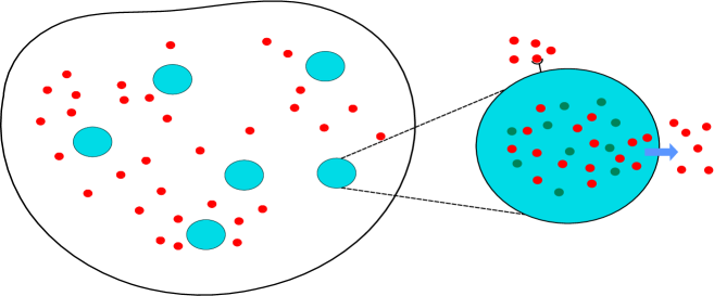
Figure 1: Schematic diagram showing the intracellular reactions and external bulk diffusion of the signal. The small shaded regions are the signaling compartments or cells.

Before discussing our main results, we first formulate and non-dimensionalize our coupled cell-bulk model assuming that there is only one signaling compartment $\Omega_{0}$ inside the two-dimensional domain $\Omega$. The corresponding dimensionless model for $m>1$ small signaling cells is given in (2.1). Fig. 1 shows a schematic plot of the geometry for $m$ small cells. We assume that the cell can release a specific signaling molecule into the bulk region exterior to the cell, and that this secretion is regulated by both the extracellular concentration of the molecule together with its number density inside the cell. If ${\mathcal{U}}({\boldsymbol{X}},T)$ represents the concentration of the signaling molecule in the bulk region $\Omega\backslash\Omega_{0}$, then its spatial-temporal evolution in this region is assumed to be governed by the PDE model

$${\mathcal{U}}_{T} =D_{B}\Delta_{\boldsymbol{X}}{\mathcal{U}}-k_{B}{\mathcal{U}}\,,\qquad\boldsymbol{X}\in\Omega\backslash\Omega_{0}\,;\qquad\partial_{n_{\boldsymbol{X}}}{\mathcal{U}}=0\,,\qquad\boldsymbol{X}\in\partial\Omega\,,$$ (1.1a)

$$D_{B}\partial_{n_{\boldsymbol{X}}}{\mathcal{U}} =\beta_{1}{\mathcal{U}}-\beta_{2}{\mu}^{1}\,,\;\;\quad\boldsymbol{X}\in\partial\Omega_{0}\,,$$

where, for simplicity, we assume that the signaling compartment $$\Omega_{0}\in\Omega \sigma \boldsymbol{X}_{0}\in\Omega n \boldsymbol{\mu}\equiv(\mu^{1},\ldots,\mu^{n})^{T} n \partial\Omega_{0}$$ is a disk of radius centered at some . Inside the cell we assume that there are interacting species whose dynamics are governed by -ODEs, with a source term representing the exchange of material across the cell membrane , of the form

$$\frac{d\boldsymbol{\mu}}{dT}=k_{R}\mu_{c}\boldsymbol{F}\left({{\boldsymbol{\mu}}/\mu_{c}}\right)+\boldsymbol{e}_{1}\int_{\partial\Omega_{0}}\left(\beta_{1}{\mathcal{U}}-\beta_{2}\mu^{1}\right)\,dS_{\boldsymbol{X}}\,,$$ (1.1b)

where $\boldsymbol{e}_{1}\equiv(1,0,\dots,0)^{T}$. Here $\boldsymbol{\mu}$ is the total amount of the $n$ species inside the cell, while $k_{R}>0$ is the reaction rate for the dimensionless intracellular dynamics ${\boldsymbol{F}}(\boldsymbol{u})$. The scalar $\mu_{c}>0$ is a typical value for $\boldsymbol{\mu}$.

In this coupled cell-bulk model, $D_{B}>0$ is the diffusion coefficient for the bulk process, $k_{B}$ is the rate at which the signaling molecule is degraded in the bulk, while $\beta_{1}>0$ and $\beta_{2}>0$ are the dimensional influx (eflux) constants modeling the permeability of the cell wall. In addition, $\partial_{n_{\boldsymbol{X}}}$ denotes either the outer normal derivative of $\Omega$, or the outer normal to $\Omega_{0}$ (which points inside the bulk region). The flux $\beta_{1}{\mathcal{U}}-\beta_{2}\mu^{1}$ on the cell membrane models the influx of the signaling molecule into the extracellular bulk region, which depends on both the external bulk concentration ${\mathcal{U}}({\boldsymbol{X}},T)$ at the cell membrane $\partial\Omega_{0}$ as well as on the intracellular concentration $\mu^{1}$ within the cell. We assume that only one of the intracellular species, $\mu^{1}$, is capable of being transported across the cell membrane $\partial\Omega_{0}$ into the bulk. We remark that a related class of models was formulated and analyzed in [1] and [2] in their study of the initiation of the biological cell cycle, where the dynamically active compartment is the nucleus of the biological cell.

Next, we introduce our scaling assumption that the radius $\sigma$ of the cell is small compared to the radius of the domain, so that $\epsilon\equiv{\sigma/L}\ll 1$, where $L$ is the length-scale of $\Omega$. However, in order that the signaling compartment has a non-negligible effect on the bulk process, we need to assume that $\beta_{1}$ and $\beta_{2}$ are both ${\mathcal{O}}(\epsilon^{-1})\gg 1$ as $\epsilon\to 0$. In this way, in Appendix A we show that (1.1) reduces to the dimensionless coupled system

$$\tau{U}_{t} =D\Delta_{\boldsymbol{x}}{U}-{U}\,,\qquad\boldsymbol{x}\in{\Omega}\backslash{\Omega}_{0}\,;\qquad\partial_{n_{\boldsymbol{x}}}{U}=0\,,\qquad\boldsymbol{x}\in\partial{\Omega}\,,$$ (1.2a)

$$\epsilon D\partial_{n_{\boldsymbol{x}}}{U} =d_{1}{U}-d_{2}u^{1}\,,\;\;\quad\boldsymbol{x}\in\partial{\Omega}_{0}\,,$$

where $${\Omega}_{0} \epsilon\ll 1 x_{0}\in{\Omega}$$ is a disk of radius centered at some . The bulk process is coupled to the intracellular dynamics by

$$\frac{d\boldsymbol{u}}{dt}=\boldsymbol{F}\left(\boldsymbol{u}\right)+\frac{\boldsymbol{e}_{1}}{\tau\epsilon}\int_{\partial{\Omega}_{0}}\left(d_{1}{U}-d_{2}u^{1}\right)\,dS_{\boldsymbol{x}}\,.$$ (1.2b)

The four ${\mathcal{O}}(1)$ dimensionless parameters in (1.2) are $\tau$, $D$, $d_{1}$, and $d_{2}$, defined by

$$\tau\equiv\frac{k_{R}}{k_{B}}\,,\qquad D\equiv\frac{D_{B}}{k_{B}L^{2}}\,,\qquad\beta_{1}\equiv\left(k_{B}L\right)\frac{d_{1}}{\epsilon}\,,\qquad\beta_{2}\equiv\left(\frac{k_{B}}{L}\right)\frac{d_{2}}{\epsilon}\,.$$ (1.3)

We remark that the limit $\tau\ll 1$ ($\tau\gg 1$) corresponds to when the intracellular dynamics is very slow (fast) with respect to the time-scale of degradation of the signaling molecule in the bulk. The limit $D\gg 1$ corresponds to when the bulk diffusion length $\sqrt{D_{B}/k_{B}}$ is large compared to the length-scale $L$ of the confining domain.

A related class of coupled cell-bulk models involving two bulk diffusing species, and where the cells, centered at specific spatial sites, are modeled solely by nonlinear flux boundary conditions, have been used to model cellular signal cascades (cf. [14], [15]), and the effect of catalyst particles on chemically active substrates (cf. [22], [19]). In contrast to these nonlinear flux-based models, in the coupled cell-bulk models of [17] and [18], and the one considered herein, the cells are not quasi-static but are, instead, dynamically active units. Our main goal for (1.2) and (2.1) is to determine conditions that lead to the triggering of synchronized oscillations between the dynamically active cells. Related 1-D cell-bulk models, where the cells are dynamically active units at the ends of a 1-D spatial domain, have been analyzed in [7]–[10].

Our analysis of the 2-D coupled cell-bulk model (1.2), and its multi-cell counterpart (2.1), which extends the 3-D modeling paradigm of [17] and [18], has the potential of providing a theoretical framework to model quorum sensing behavior in experiments performed in petri dishes, where cells live on a thin substrate. In contrast to the assumption of only one active intracellular component used in [17] and [18], in our study we will allow for $m$ small spatially segregated cells with multi-component intracellular dynamics. We will show for our 2-D case that the communication between small cells through the diffusive medium is much stronger than in 3-D, and leads in certain parameter regimes to the triggering of synchronous oscillations, which otherwise would not be present in the absence of any cell-bulk coupling. In addition, when $D={\mathcal{O}}(1)$, we show that the spatial configuration of small cells in the domain is an important factor in triggering collective synchronous temporal instabilities in the cells.

The outline of this paper is as follows. In §2 we use the method of matched asymptotic expansions to construct steady-state solutions to our 2-D multi-cell-bulk model (2.1), and we derive a globally coupled eigenvalue problem whose spectrum characterizes the stability properties of the steady-state. In our 2-D analysis, the interaction between the cells is of order $\nu\equiv-1/\log\epsilon$, where $\epsilon\ll 1$ is the assumed common radius of the small circular cells. In the distinguished limit where the bulk diffusion coefficient $D$ is of the asymptotic order $D=\mathcal{O}(\nu^{-1})$, in §3 we show that the leading order approximate steady-state solution and the associated linear stability problem are both independent of the spatial configurations of cells and the shape of the domain. In this regime, we then show that the steady-state solution can be destabilized by either a synchronous perturbation in the cells or by $m-1$ possible asynchronous modes of instability. In §3 leading-order-in-$\nu$ limiting spectral problems when $D={D_{0}/\nu}$, with $\nu\ll 1$, for both these classes of instabilities are derived. In §4, we illustrate our theory for various intracellular dynamics. When there is only a single dynamically active intracellular component, we show that no triggered oscillations can occur. For two specific intracellular reaction kinetics involving two local species, modeled either by Sel’kov or Fitzhugh-Nagumo (FN) dynamics, in §4 we perform detailed analysis to obtain Hopf bifurcation boundaries, corresponding to the onset of either synchronous or asynchronous oscillations, in various parameter planes. In addition to this detailed stability analysis for the $D=\mathcal{O}(\nu^{-1})$ regime, in §5 we show for the case of one cell that when $D\gg\mathcal{O}(\nu^{-1})$ the coupled cell-bulk model is effectively well-mixed and its solutions can be well-approximated by a finite-dimensional system of nonlinear ODEs. The analytical and numerical study of these limiting ODEs in §5 reveals that their steady-states can be destabilized through a Hopf bifurcation. Numerical bifurcation software is then used to show the existence of globally stable time-periodic solution branches that are intrinsically due to the cell-bulk coupling. For the $D={\mathcal{O}}(1)$ regime, where the spatial configuration of the cells in the domain is an important factor, in §6 we perform a detailed stability analysis for a ring-shaped pattern of cells that is concentric within the unit disk. For this simple spatial configuration of cells, phase diagrams in the $\tau$ versus $D$ parameter space, for various ring radii, characterizing the existence of either synchronous or asynchronous oscillatory instabilities, are obtained for the case of Sel’kov intracellular dynamics. These phase diagrams show that triggered synchronous oscillations can occur when cells become more spatially clustered. In §6 we also provide a clear example of quorom sensing behavior, characterized by the triggering of collective dynamics only when the number of cells exceeds a critical threshold. Finally, in §7 we briefly summarize our main results and discuss some open directions.

Our analysis of synchronous and asynchronous instabilities for (2.1) in the $D={\mathcal{O}}(\nu^{-1})$ regime, where the stability thresholds are to, to leading-order, independent of the spatial configuration of cells, has some similarities with the stability analysis of [27], [28], [25], and [3] (see also the references therein) for localized spot solutions to various activator-inhibitor RD systems with short range activation and long-range inhibition. In this RD context, when the inhibitor diffusivity is of the order ${\mathcal{O}}(\nu^{-1})$, localized spot patterns can be destabilized by either synchronous or asynchronous perturbations, with the stability thresholds being, to leading-order in $\nu$, independent of the spatial configuration of the spots in the domain. The qualitative reason for this similarity between the coupled cell-bulk and localized spot problems is intuitively rather clear. In the RD context, the inhibitor diffusion field is the long-range “bulk” diffusion field, which mediates the interaction between the “dynamically active units”, consisting of $m$ spatially segregated localized regions of high activator concentration, each of which is is self-activating. In this RD context, asynchronous instabilities lead to asymmetric spot patterns, while synchronous oscillatory instabilities lead to collective temporal oscillations in the amplitudes of the localized spots (cf. [27], [28], [25], and [3]). A more detailed discussion of this analogy is given in Remark 3.1.

Finally, we remark that the asymptotic framework for the construction of steady-state solutions to the cell-bulk model (2.1), and the analysis of their linear stability properties, relies heavily on the methodology of strong localized perturbation theory (cf. [26]). Related problems where such techniques are used include [13], [23], [14], and [15].

2 Analysis of the Dimensionless 2-D Cell-Bulk System

We first generalize the one-cell model of §1 by formulating a class of dimensionless coupled cell-bulk dynamics that contains $m$ small, disjoint, cells or compartments that are scattered inside the bounded two-dimensional domain $\Omega$. We assume that each cell is a small disk of a common radius $\epsilon\ll 1$ that shrinks to a point $\boldsymbol{x}_{j}\in\Omega$ as $\epsilon\to 0$, and that are well-separated in the sense that dist$(\boldsymbol{x}_{i},\boldsymbol{x}_{j})=O(1)$ for $i\neq j$ and dist$(\boldsymbol{x}_{j},\partial\Omega)=O(1)$ for $j=1,\ldots,m$, as $\epsilon\to 0$.

As motivated by the dimensional reasoning provided in §1, if $U({\boldsymbol{x}},t)$ is the dimensionless concentration of the signaling molecule in the bulk region between the cells, then in this region it satisfies the dimensionless PDE

$$\tau U_{t} =D\Delta U-U\,,\qquad\boldsymbol{x}\in\Omega\backslash\cup_{j=1}^{m}\Omega_{\epsilon_{j}}\,;\qquad\partial_{n}U=0\,,\qquad\boldsymbol{x}\in\partial\Omega\,,$$ (2.1a)

$$\epsilon D\partial_{n_{j}}U =d_{1}U-d_{2}u^{1}_{j}\,,\;\;\quad\boldsymbol{x}\in\partial\Omega_{\epsilon_{j}}\,,\quad j=1,\ldots,m\,.$$

Here $$D>0 d_{1}>0 d_{2}>0 \partial_{n} \Omega \partial_{n_{j}} \Omega_{\epsilon_{j}} \Omega_{\epsilon_{j}} \Omega d_{1}U-d_{2}u^{1}_{j} U({\boldsymbol{x}},t) \partial\Omega_{\epsilon_{j}} u_{j}^{1} j m n$$ is the effective diffusivity of the bulk, and are the dimensionless influx (eflux) constants modeling the permeability of the cell membrane, denotes the outer normal derivative of , and denotes the outer normal to each , which points inside the bulk region. The signaling cell, or compartment, is assumed to lie entirely within . The flux on each cell membrane models the influx of the signaling molecule into the extracellular bulk region, which depends on both the external bulk concentration at the cell membrane as well as on the amount of one of the intracellular species within the -th cell. We suppose that inside each of the cells there are interacting species, with intracellular dynamics

$$\frac{d\boldsymbol{u}_{j}}{dt}=\boldsymbol{F}_{j}(\boldsymbol{u}_{j})+\frac{\boldsymbol{e}_{1}}{\epsilon\tau}\int_{\partial\Omega_{\epsilon_{j}}}(d_{1}U-d_{2}u^{1}_{j})\,ds\,,$$ (2.1b)

where $\boldsymbol{e}_{1}\equiv(1,0,\dots,0)^{T}$. Here $\boldsymbol{u}_{j}=(u^{1}_{j},\dots,u^{n}_{j})^{T}$ is the mass of the $n$ species inside the $j$-th cell and $\boldsymbol{F}_{j}(\boldsymbol{u}_{j})$ is the vector nonlinearity modeling the reaction dynamics within the $j$-th cell. The integration in (2.1b) is over the boundary $\partial\Omega_{\epsilon_{j}}$ of the compartment. Since its perimeter has length $|\partial\Omega_{\epsilon_{j}}|={\mathcal{O}}(\epsilon)$, this source term for the ODE in (2.1b) is ${\mathcal{O}}(1)$ as $\epsilon\to 0$. The dimensionless parameters $D$, $\tau$, $d_{1}$, and $d_{2}$, are related to their dimensional counterparts by (1.3). The qualitative interpretation of the limits $\tau\ll 1$, $\tau\gg 1$, and $D\gg 1$, were discussed following (1.3).

2.1 The Steady-State Solution for the $m$ Cells System

We construct a steady-state solution to (2.1) under the assumption that the cells are well-separated in the sense described preceding (2.1). In §2.2 we will then formulate the linear stability problem for this steady-state solution.

Since in an ${\mathcal{O}}(\epsilon)$ neighborhood near each cell the solution $U$ has a sharp spatial gradient, we use the method of matched asymptotic expansions to construct the steady-state solution to (2.1). In the inner region near the $j$-th cell, we introduce the local variables $U_{j}$ and $\boldsymbol{y}$, defined by $\boldsymbol{y}=\epsilon^{-1}(\boldsymbol{x}-\boldsymbol{x}_{j})$ and $U_{j}(\boldsymbol{y})=U({\boldsymbol{x}_{j}}+\epsilon{\boldsymbol{y}})\,,$ so that (2.1a) transforms to

$$D\Delta_{\boldsymbol{y}}U_{j}-\epsilon^{2}U_{j}=0\,,\qquad|\boldsymbol{y}|>1\,;\qquad D\partial_{n_{j}}U_{j}=d_{1}U_{j}-d_{2}u^{1}_{j}\,,\qquad|\boldsymbol{y}|=1\,.$$ (2.2)

We look for a radially symmetric solution to (2.2) in the form $U_{j}=U_{j}(\rho)$, where $\rho\equiv|{\boldsymbol{y}}|$ and $\Delta_{\boldsymbol{y}}=\partial_{\rho\rho}+\rho^{-1}\partial_{\rho}$ denotes the radially symmetric part of the Laplacian. Therefore, to leading order, we have that $U_{j}(\rho)$ satisfies

$$\partial_{\rho\rho}U_{j}+\rho^{-1}\partial_{\rho}U_{j}=0\,,\qquad 1<\rho<\infty\,;\qquad D\frac{\partial U_{j}}{\partial\rho}=d_{1}U_{j}-d_{2}u^{1}_{j}\,,\qquad\rho=1\,.$$ (2.3)

The solution to (2.3) in terms of a constant $S_{j}$, referred to as the source strength of the $j$-th cell, is

$$U_{j}=S_{j}\log\rho+\chi_{j}\,,\qquad\chi_{j}=\frac{1}{d_{1}}(DS_{j}+d_{2}u^{1}_{j})\,,\qquad j=1,\dots,m\,.$$ (2.4)

The constant $S_{j}$ will be determined below upon matching the inner solutions to the outer solution.

From the steady-state of the intracellular dynamics (2.1b) inside each cell, we find that the source strength $S_{j}$ and the steady-state solution $\boldsymbol{u}_{j}$ satisfy the nonlinear algebraic system

$$\boldsymbol{F}_{j}(\boldsymbol{u}_{j})+\frac{2\pi D}{\tau}S_{j}\boldsymbol{e}_{1}=0\,.$$ (2.5)

In principle, we can determine $u^{1}_{j}$ in terms of the unknown $S_{j}$ as $u^{1}_{j}=u^{1}_{j}(S_{j})$. The other values $u_{2}^{j},\dots,u_{n}^{j}$ also depend on $S_{j}$. Next, in terms of $u_{j}^{1}$, we will derive a system of algebraic equations for $S_{1},\ldots,S_{m}$, which is coupled to (2.5).

Upon matching the far-field behavior of the inner solution (2.4) to the outer solution, we obtain the outer problem

$$\Delta U-\varphi_{0}^{2}U =0\,,\qquad\boldsymbol{x}\in\Omega\backslash\{{\boldsymbol{x}_{1},\ldots,\boldsymbol{x}_{m}\}}\,;\qquad\partial_{n}U=0\,,\qquad\boldsymbol{x}\in\partial\Omega\,,$$ (2.6)

$$U \sim S_{j}\log|\boldsymbol{x}-\boldsymbol{x}_{j}|+\frac{S_{j}}{\nu}+\chi_{j}\,,\quad\text{as }\;\boldsymbol{x}\rightarrow\boldsymbol{x}_{j}\,,\quad j=1,\ldots,m\,,$$

where we have defined $\varphi_{0}$ and $\nu\ll 1$ by

$$\varphi_{0}\equiv 1/\sqrt{D}\,,\qquad\nu\equiv{-1/\log\epsilon}\,.$$ (2.7)

We remark that the singularity condition in (2.6) is derived by matching the outer solution for $U$ to the far-field behavior of the inner solution (2.4). We then introduce the reduced-wave Green’s function $G(\boldsymbol{x};\boldsymbol{x}_{j})$ satisfying

$$\Delta G-\varphi_{0}^{2}G=-\delta(\boldsymbol{x}-\boldsymbol{x}_{j})\,,\qquad\boldsymbol{x}\in\Omega\,;\qquad\partial_{n}G=0\,,\qquad\boldsymbol{x}\in\partial\Omega\,.$$ (2.8a)

As $$\boldsymbol{x}\rightarrow\boldsymbol{x}_{j}$$, this Green’s function has the local behavior

$$G(\boldsymbol{x};\boldsymbol{x}_{j})\sim-\frac{1}{2\pi}\log|\boldsymbol{x}-\boldsymbol{x}_{j}|+R_{j}+o(1)\,,\qquad\mbox{as}\quad\boldsymbol{x}\rightarrow\boldsymbol{x}_{j}\,,$$ (2.8b)

where $R_{j}=R_{j}(\boldsymbol{x}_{j})$ is called the regular part of $G(\boldsymbol{x};\boldsymbol{x}_{j})$ at $\boldsymbol{x}=\boldsymbol{x}_{j}$. In terms of $G(\boldsymbol{x};\boldsymbol{x}_{j})$, the solution to (2.6) is

$$U(\boldsymbol{x})=-2\pi\sum_{i=1}^{m}S_{i}G(\boldsymbol{x},\boldsymbol{x}_{i})\,.$$ (2.9)

By expanding $U$ as $\boldsymbol{x}\rightarrow\boldsymbol{x}_{j}$, and equating the resulting expression with the required singularity behavior in (2.6), we obtain the following algebraic system for $\boldsymbol{S}=(S_{1},\ldots,S_{m})^{T}$, which we write in matrix form as

$$\left(1+\frac{D\nu}{d_{1}}\right)\boldsymbol{S}+2\pi\nu{\mathcal{G}}\boldsymbol{S}=-\frac{d_{2}}{d_{1}}\nu\boldsymbol{u}^{1}\,.$$ (2.10)

Here the Green’s matrix ${\mathcal{G}}$, with matrix entries $({\mathcal{G}})_{ij}$, and the vector $\boldsymbol{u}^{1}$, whose $j$-th element is the first local species in the $j$-th cell, are given by

$$({\mathcal{G}})_{ii}=R_{i}\,,\qquad({\mathcal{G}})_{ij}=G(\boldsymbol{x}_{i};\boldsymbol{x}_{j})\equiv G_{ij}\,,\quad i\neq j\,;\qquad\boldsymbol{u}^{1}\equiv\left(u_{1}^{1},\ldots,u_{m}^{1}\right)^{T}\,.$$

Since $G_{ji}=G_{ij}$, by the reciprocity of the Green’s function, ${\mathcal{G}}$ is a symmetric matrix.

Together with (2.5), (2.10) provides an approximate steady-state solution for $\boldsymbol{u}$, which is coupled to the source strengths $\boldsymbol{S}$. It is rather intractable analytically to write general conditions on the nonlinear kinetics to ensure the existence of a solution to the coupled algebraic system (2.5) and (2.10). As such, in §4 below we will analyze in detail some specific choices for the nonlinear kinetics. We remark that even if we make the assumption that the nonlinear kinetics in the cells are identical, so that $\boldsymbol{F}_{j}=\boldsymbol{F}$ for $j=1,\ldots,m$, we still have that $S_{j}$ and $\boldsymbol{u}^{1}$ depend on $j$ through the Green’s interaction matrix ${\mathcal{G}}$, which depends on the spatial configuration $\{{\boldsymbol{x}_{1},\ldots,\boldsymbol{x}_{m}\}}$ of the cells within $\Omega$.

In summary, after solving the nonlinear algebraic system (2.5) and (2.10), the approximate steady-state solution for $U$ is given by (2.9) in the outer region, defined at ${\mathcal{O}}(1)$ distances from the cells, and (2.4) in the neighborhood of each cell. This approximate steady-state solution is accurate to all orders in $\nu$, since our analysis has effectively summed an infinite order logarithmic expansion in powers of $\nu$ for the steady-state solution. Related 2-D problems where infinite logarithmic expansions occur for various specific applications were analyzed in [13] and [23] (see also the references therein).

2.2 Formulation of the Linear Stability Problem

Next, we consider the linear stability of the steady-state solution constructed in the previous subsection. We perturb this steady-state solution, denoted here by $U_{e}(\boldsymbol{x})$ in the bulk region and $\boldsymbol{u}_{e,j}$ in the $j$-th cell as $U=U_{e}+e^{\lambda t}\eta({\boldsymbol{x}})$ and $\boldsymbol{u}_{j}=\boldsymbol{u}_{e,j}+e^{\lambda t}\boldsymbol{\phi}_{j}$. Upon substituting this perturbation into (2.1), we obtain in the bulk region that

$$\tau\lambda\eta =D\Delta\eta-\eta\,,\qquad\boldsymbol{x}\in\Omega\backslash\cup_{j=1}^{m}\Omega_{\epsilon_{j}}\,;\qquad\partial_{n}\eta=0\,,\qquad\boldsymbol{x}\in\partial\Omega\,,$$ (2.11a)

$$\epsilon D\partial_{n_{j}}\eta =d_{1}\eta-d_{2}\boldsymbol{\phi}_{j}^{1}\,,\qquad\boldsymbol{x}\in\partial\Omega_{\epsilon_{j}}\,,\qquad j=1,\ldots,m\,.$$

Within the $$j$$-th cell the linearized problem is

$$\lambda\phi_{j}=J_{j}\phi_{j}+\frac{\boldsymbol{e}_{1}}{\epsilon\tau}\int_{\partial\Omega_{\epsilon_{j}}}\left(d_{1}\eta-d_{2}\boldsymbol{\phi}_{j}^{1}\right)\,ds\,,$$ (2.11b)

where $J_{j}$ denotes the Jacobian matrix of the nonlinear kinetics $\boldsymbol{F}_{j}$ evaluated at $\boldsymbol{u}_{e,j}$. We now study (2.11) in the limit $\epsilon\to 0$ using the method of matched asymptotic expansions. The analysis will provide a limiting globally coupled eigenvalue problem for $\lambda$, from which we can investigate possible instabilities.

In the inner region near the $j$-th cell, we introduce the local variables $\boldsymbol{y}=\epsilon^{-1}(\boldsymbol{x}-\boldsymbol{x}_{j})$, with $\rho=|{\boldsymbol{y}}|$, and let $\eta_{j}(\boldsymbol{y})=\eta(\boldsymbol{x}_{j}+\epsilon\boldsymbol{y})$. We will look for the radially symmetric eigenfunction $\eta_{j}$ in the inner variable $\rho$. Then, from (2.11a), upon neglecting higher order algebraic terms in $\epsilon$, the leading order inner problem becomes

$$\partial_{\rho\rho}\eta_{j}+\rho^{-1}\partial_{\rho}\eta_{j}=0\,,\qquad 1<\rho<\infty\,;\qquad D\frac{\partial\eta_{j}}{\partial\rho}=d_{1}\eta_{j}-d_{2}\phi_{j}^{1}\,,\qquad\rho=1\,,$$ (2.12)

which has the solution

$$\eta_{j}=c_{j}\log\rho+B_{j}\,,\qquad B_{j}=\frac{1}{d_{1}}(Dc_{j}+d_{2}\phi_{j}^{1})\,,$$ (2.13)

where $c_{j}$ is an unknown constant to be determined. Then, upon substituting (2.13) into (2.11b), we obtain that

$$(J_{j}-\lambda I)\boldsymbol{\phi}_{j}+\frac{2\pi D}{\tau}c_{j}\boldsymbol{e}_{1}=0\,,\qquad j=1,\ldots,m\,.$$ (2.14)

In the outer region, defined at ${\mathcal{O}}(1)$ distances from the cells, the outer problem for the eigenfunction $\eta(\boldsymbol{x})$ is

$$\Delta\eta-\frac{(1+\tau\lambda)}{D}\eta=0,\qquad\boldsymbol{x}\in\Omega\backslash\{{\boldsymbol{x}_{1},\ldots,\boldsymbol{x}_{m}\}}\,;\qquad\partial_{n}\eta=0,\qquad\boldsymbol{x}\in\partial\Omega\,,$$ (2.15)

$$\eta\sim c_{j}\log|\boldsymbol{x}-\boldsymbol{x}_{j}|+\frac{c_{j}}{\nu}+B_{j},\qquad\mbox{as}\quad\boldsymbol{x}\rightarrow\boldsymbol{x}_{j}\,,\quad j=1,\ldots,m\,,$$

where $\nu\equiv-{1/\log\epsilon}$. We remark that the singularity condition in (2.15) as $\boldsymbol{x}\rightarrow\boldsymbol{x}_{j}$ is derived by matching the outer solution for $\eta$ to the far-field behavior of the inner solution (2.13). To solve (2.15), we introduce the eigenvalue-dependent Green’s function $G_{\lambda}(\boldsymbol{x};\boldsymbol{x}_{j})$, which satisfies

$$\Delta G_{\lambda}-\varphi_{\lambda}^{2}G_{\lambda}=-\delta(\boldsymbol{x}-\boldsymbol{x}_{j}),\qquad\boldsymbol{x}\in\Omega\,;\qquad\partial_{n}G_{\lambda}=0\,,\qquad\boldsymbol{x}\in\partial\Omega\,,$$ (2.16)

$$G_{\lambda}(\boldsymbol{x};\boldsymbol{x}_{j})\sim-\frac{1}{2\pi}\log|\boldsymbol{x}-\boldsymbol{x}_{j}|+R_{\lambda,j}+o(1)\,,\qquad\mbox{as}\quad\boldsymbol{x}\rightarrow\boldsymbol{x}_{j}\,,$$

where $R_{\lambda,j}\equiv R_{\lambda}(\boldsymbol{x}_{j})$ is the regular part of $G_{\lambda}$ at $\boldsymbol{=}\boldsymbol{x}_{j}$. Here we have defined $\varphi_{\lambda}$ by

$$\varphi_{\lambda}\equiv\sqrt{\frac{1+\tau\lambda}{D}}\,.$$ (2.17)

We must choose the principal branch of $\varphi_{\lambda}$, which ensures that $\varphi_{\lambda}$ is analytic in $\mbox{Re}(\lambda)>0$. For the case of an asymptotically large domain $\Omega$, this choice for the branch cut, for which $\mbox{Re}(\theta_{\lambda})>0$, also ensures that $G_{\lambda}$ decays as $|\boldsymbol{x}-\boldsymbol{x}_{j}|\to\infty$.

In terms of $G_{\lambda}(\boldsymbol{x};\boldsymbol{x}_{j})$, we can represent the outer solution $\eta(\boldsymbol{x})$ satisfying (2.15), as

$$\eta(\boldsymbol{x})=-2\pi\sum_{i=1}^{m}c_{i}G_{\lambda}(\boldsymbol{x},\boldsymbol{x}_{i})\,.$$ (2.18)

By matching the singularity condition at $\boldsymbol{x}\rightarrow\boldsymbol{x}_{j}$, we obtain a system of equations for $c_{j}$ as

$$c_{j}+\nu B_{j}=-2\pi\nu\left(c_{j}R_{\lambda_{j}}+\sum_{i\neq j}^{m}c_{i}G_{\lambda,ij}\right)\,,\qquad j=1,\ldots,m\,,$$ (2.19)

where $G_{\lambda,ij}\equiv G_{\lambda}(\boldsymbol{x}_{j};\boldsymbol{x}_{i})$. Upon recalling that $B_{j}=\frac{1}{d_{1}}(Dc_{j}+d_{2}\phi_{j}^{1})$ from (2.13), we can rewrite (2.19) in matrix form in terms of $\boldsymbol{c}=(c_{1},\ldots,c_{m})^{T}$ as

$$\left(1+\frac{D\nu}{d_{1}}\right)\boldsymbol{c}+\frac{d_{2}}{d_{1}}\nu\boldsymbol{\phi}^{1}+2\pi\nu{\mathcal{G}}_{\lambda}\boldsymbol{c}=0\,.$$ (2.20)

Here we have defined the symmetric Green’s matrix ${\mathcal{G}}_{\lambda}$, with matrix entries $({\mathcal{G}})_{\lambda,ij}$, and the vector $\boldsymbol{\phi}^{1}$ by

$$({\mathcal{G}})_{\lambda,ii}=R_{\lambda,i}\,,\qquad({\mathcal{G}})_{\lambda,ij}=G_{\lambda}(\boldsymbol{x}_{i};\boldsymbol{x}_{j})\equiv G_{\lambda,ij}\,,\quad i\neq j\,;\qquad\boldsymbol{\phi}^{1}\equiv\left(\phi_{1}^{1},\ldots,\phi_{m}^{1}\right)^{T}\,.$$ (2.21)

The $j$-th entry of the vector $\phi^{1}=(\phi^{1}_{1},\cdots,\phi^{1}_{m})^{T}$ is simply the first element in the eigenvector for the $j$-th cell. Together with (2.14), the system (2.20) will yield an eigenvalue problem for $\lambda$ with eigenvector $\boldsymbol{c}$.

Next, we calculate $\phi_{1}$ in terms of $\boldsymbol{c}$ from (2.14) and then substitute the resulting expression into (2.20). If $\lambda$ is not an eigenvalue of $J_{j}$, (2.14) yields that $\boldsymbol{\phi}_{j}=2\pi D\tau^{-1}(\lambda I-J_{j})^{-1}c_{j}\boldsymbol{e}_{1}$. Upon taking the dot product with the $n$-vector $\boldsymbol{e}_{1}=(1,0,\ldots,0)^{T}$, we get $\phi_{j}^{1}=2\pi D\tau^{-1}c_{j}{\boldsymbol{e}_{1}}^{T}(\lambda I-J_{j})^{-1}{\boldsymbol{e}_{1}}$, which yields in vector form that

$$\phi^{1}=\frac{2\pi D}{\tau}{\mathcal{K}}\boldsymbol{c}\,,$$ (2.22a)

where $${\mathcal{K}}={\mathcal{K}}(\lambda) m\times m$$ is the diagonal matrix with diagonal entries

$${\mathcal{K}}_{j}={\boldsymbol{e}_{1}}^{T}(\lambda I-J_{j})^{-1}{\boldsymbol{e}_{1}}=\frac{1}{\det(\lambda I-J_{j})}\boldsymbol{e}_{1}M_{j}^{T}\boldsymbol{e}_{1}=\frac{M_{j,11}}{\det(\lambda I-J_{j})}\,.$$ (2.22b)

Here $M_{j}$ is the $n\times n$ matrix of cofactors of the matrix $\lambda I-J_{j}$, with $M_{j,11}$ denoting the matrix entry in the first row and first column of $M_{j}$, given explicitly by

$$M_{j,11}=M_{j,11}(\lambda)\equiv\det\left(\begin{array}[]{ccc}\lambda-\frac{\partial{F}_{j}^{2}}{\partial u_{2}}\Big{|}_{\boldsymbol{u}=\boldsymbol{u}_{e,j}},&\cdots,&-\frac{\partial{F}_{j}^{2}}{\partial u_{n}}\Big{|}_{\boldsymbol{u}=\boldsymbol{u}_{e,j}}\\ \cdots,&\cdots,&\cdots\\ -\frac{\partial{F}_{j}^{n}}{\partial u_{2}}\Big{|}_{\boldsymbol{u}=\boldsymbol{u}_{e,j}},&\cdots,&\lambda-\frac{\partial{F}_{j}^{n}}{\partial u_{n}}\Big{|}_{\boldsymbol{u}=\boldsymbol{u}_{e,j}}\end{array}\right)\,.$$ (2.23)

Here ${F}_{j}^{2},\ldots,{F}_{j}^{n}$ denote the components of the vector $\boldsymbol{F}_{j}\equiv(F_{j}^{1},\ldots,F_{j}^{n})^{T}$, characterizing the intracellular kinetics.

Next, upon substituting (2.22a) into (2.20), we obtain the homogeneous $m\times m$ linear system

$${\mathcal{M}}\boldsymbol{c}=\boldsymbol{0}\,,$$ (2.24a)

where the $$m\times m {\mathcal{M}}={\mathcal{M}}(\lambda)$$ matrix is defined by

$$\mathcal{M}\equiv\left(1+\frac{D\nu}{d_{1}}\right)I+2\pi\nu\frac{d_{2}}{d_{1}{\tau}}D{\mathcal{K}}+2\pi\nu{\mathcal{G}}_{\lambda}\,.$$ (2.24b)

In (2.24b), the diagonal matrix ${\mathcal{K}}$ has diagonal entries (2.22b), and ${\mathcal{G}}_{\lambda}$ is the Green’s interaction matrix defined in (2.21), which depends on $\lambda$ as well as on the spatial configuration $\{{\boldsymbol{x}_{1},\ldots,\boldsymbol{x}_{m}\}}$ of the centers of the small cells within $\Omega$.

We refer to (2.24) as the globally coupled eigenvalue problem (GCEP). In the limit $\epsilon\to 0$, we conclude that $\lambda$ is a discrete eigenvalue of the linearized problem (2.11) if and only if $\lambda$ is a root of the transcendental equation

$$\det\mathcal{M}=0\,.$$ (2.25)

To determine the region of stability, we must seek conditions to ensure that all such eigenvalues satisfy $\mbox{Re}(\lambda)<0$. The corresponding eigenvector $\boldsymbol{c}$ of (2.24) gives the spatial information for the eigenfunction in the bulk via (2.18).

We now make some remarks on the form of the GCEP. We first observe from (2.24b) that when $D={\mathcal{O}}(1)$, then to leading-order in $\nu\ll 1$, we have that ${\mathcal{M}}\sim I+{\mathcal{O}}(\nu)$. As such, when $D={\mathcal{O}}(1)$, we conclude that to leading order in $\nu$ there are no discrete eigenvalues of the linearized problem with $\lambda={\mathcal{O}}(1)$, and hence no ${\mathcal{O}}(1)$ time-scale instabilities. However, since $\nu={-1/\log\epsilon}$ is not very small unless $\epsilon$ is extremely small, this prediction of no instability in the $D={\mathcal{O}}(1)$ regime may be somewhat misleading at small finite $\epsilon$. In §6 we determine the roots of (2.25) numerically, without first assuming that $\nu\ll 1$, for a ring-shaped pattern of cells within the unit disk $\Omega$, for which the Green’s matrix is cyclic. In the next section we will consider the distinguished limit $D={\mathcal{O}}(\nu^{-1})\gg 1$ for (2.24b) where the linearized stability problem becomes highly tractable analytically.

3 The Distinguished Limit of $D={\mathcal{O}}(\nu^{-1})\gg 1$

In the previous section, we constructed the steady-state solution for the coupled cell-bulk system (2.1) in the limit $\epsilon\to 0$ and we derived the spectral problem that characterizes the linear stability of this solution. In this section, we consider the distinguished limit where the signaling molecule in the bulk diffuses rapidly, so that $D\gg 1$. More specifically, we will consider the distinguished limit where $D={\mathcal{O}}(\nu^{-1})$, and hence for some $D_{0}={\mathcal{O}}(1)$, we set

$$D={D_{0}/\nu}\,.$$ (3.1)

For $D={\mathcal{O}}(\nu^{-1})$, we determine a leading order approximation for the steady-state solution and the associated spectral problem. To do so, we first approximate the reduced-wave Green’s function for large $D$ by writing (2.8a) as

$$\Delta G-\frac{\nu}{D_{0}}G=-\delta(\boldsymbol{x}-\boldsymbol{x}_{j})\,,\qquad\boldsymbol{x}\in\Omega\,;\qquad\partial_{n}G=0,\qquad\boldsymbol{x}\in\partial\Omega\,.$$ (3.2)

This problem has no solution when $\nu=0$. Therefore, we expand $G=G(\boldsymbol{x};\boldsymbol{x}_{j})$ for $D={D_{0}/\nu}\gg 1$ as

$$G=\frac{1}{\nu}G_{-1}+G_{0}+\nu G_{1}+\ldots\,.$$ (3.3)

Upon substituting (3.3) into (3.2), we equate powers of $\nu$ to obtain a sequence of problems for $G_{i}$ for $i=-1,0,1$. This leads to the following two-term expansion for $G(\boldsymbol{x};\boldsymbol{x}_{j})$ and its regular part $R_{j}$ in the limit $D={D_{0}/\nu}\gg 1$:

$$G(\boldsymbol{x};\boldsymbol{x}_{j})=\frac{D_{0}}{\nu|{\Omega}|}+G_{0}(\boldsymbol{x};\boldsymbol{x}_{j})+\cdots\,,\qquad R_{j}=\frac{D_{0}}{\nu|{\Omega}|}+R_{0,j}+\cdots\,.$$ (3.4)

Here $G_{0}(\boldsymbol{x};\boldsymbol{x}_{j})$, with regular part $R_{0j}$, is the Neumann Green’s function defined as the unique solution to

$$\Delta G_{0} =\frac{1}{|{\Omega}|}-\delta(\boldsymbol{x}-\boldsymbol{x}_{j})\,,\qquad\boldsymbol{x}\in\Omega\,;\qquad\partial_{n}G_{0}=0\,,\quad\boldsymbol{x}\in\partial\Omega\,;\qquad\int_{\Omega}G_{0}\>d\boldsymbol{x}=0\,,$$ (3.5)

$$G_{0}(\boldsymbol{x};\boldsymbol{x}_{j}) \sim-\frac{1}{2\pi}\log|{\boldsymbol{x}-\boldsymbol{x}_{j}}|+R_{0,j},\qquad\boldsymbol{x}\rightarrow\boldsymbol{x}_{j}\,.$$

We then substitute the expansion (3.4) and $D={D_{0}/\nu}$ into the nonlinear algebraic system (2.5) and (2.10), which characterizes the steady-state solution, to obtain that

$$\left(1+\frac{D_{0}}{d_{1}}\right)\boldsymbol{S}+\frac{2\pi mD_{0}}{|\Omega|}{\mathcal{E}}\boldsymbol{S}+2\pi\nu{\mathcal{G}}_{0}\boldsymbol{S}=-\frac{d_{2}}{d_{1}}\nu\boldsymbol{u}^{1}\,;\qquad\boldsymbol{F}_{j}(\boldsymbol{u}_{j})+\frac{2\pi D_{0}}{\tau\nu}S_{j}\boldsymbol{e}_{1}=0\,,\quad j=1,\ldots,m\,,$$ (3.6)

where the $m\times m$ matrices ${\mathcal{E}}$ and the Neumann Green’s matrix ${\mathcal{G}}_{0}$, with entries $({\mathcal{G}}_{0})_{ij}$, are defined by

$${\mathcal{E}}\equiv\frac{1}{m}\boldsymbol{e}\boldsymbol{e}^{T}\,;\qquad\left({\mathcal{G}}_{0}\right)_{ij}=G_{0}(\boldsymbol{x}_{i};\boldsymbol{x}_{j})\equiv G_{0,ij}\,,\quad i\neq j\,,\qquad\left({\mathcal{G}}_{0}\right)_{ii}=R_{0,i}\,.$$ (3.7)

Here $\boldsymbol{e}$ is the $m$-vector $\boldsymbol{e}\equiv(1,\ldots,1)^{T}$. The leading-order solution to (3.6) when $\nu\ll 1$ has the form

$$\boldsymbol{S}=\nu\boldsymbol{S}_{0}+{\mathcal{O}}(\nu^{2})\,,\qquad\boldsymbol{u}_{j}=\boldsymbol{u}_{j0}+{\mathcal{O}}(\nu)\,.$$ (3.8)

From (3.6) we conclude that $\boldsymbol{S}_{0}$ and $\boldsymbol{u}_{j0}$ satisfy the limiting leading-order nonlinear algebraic system

$$\left(1+\frac{D_{0}}{d_{1}}\right)\boldsymbol{S}_{0}+\frac{2\pi mD_{0}}{|\Omega|}{\mathcal{E}}\boldsymbol{S}_{0}=-\frac{d_{2}}{d_{1}}\boldsymbol{u}_{0}^{1}\,;\qquad\boldsymbol{F}_{j}(\boldsymbol{u}_{0j})+\frac{2\pi D_{0}}{\tau}S_{0j}\boldsymbol{e}_{1}=0\,,\quad j=1,\ldots,m\,.$$ (3.9)

Since this leading order system does not involve the Neumann Green’s matrix ${\mathcal{G}}_{0}$, we conclude that $\boldsymbol{S}_{0}$ is independent of the spatial configuration of the cells within $\Omega$.

For the special case where the kinetics $\boldsymbol{F}_{j}$ is identical for each cell, so that $\boldsymbol{F}_{j}=\boldsymbol{F}$ for $j=1,\ldots,m$, we look for a solution to (3.9) with identical source strengths, so that $S_{0j}$ and $\boldsymbol{u}_{0j}=\boldsymbol{u}_{0}$ are independent of $j$. Therefore, we write

$$\boldsymbol{S}_{0}=S_{0c}\boldsymbol{e}\,,$$ (3.10)

where $S_{0c}$ is the common source strength. From (3.9), where we use ${\mathcal{E}}\boldsymbol{e}=\boldsymbol{e}$, this yields that $S_{0c}$ and $\boldsymbol{u}_{0}$ satisfy the $m+1$ dimensional nonlinear algebraic system

$$\left(1+\frac{D_{0}}{d_{1}}+\frac{2\pi mD_{0}}{|\Omega|}\right)S_{0c}=-\frac{d_{2}}{d_{1}}u_{0}^{1}\,,\qquad\boldsymbol{F}(\boldsymbol{u}_{0})+\frac{2\pi D_{0}}{\tau}S_{0c}\boldsymbol{e}_{1}=0\,,$$ (3.11)

where $u_{0}^{1}$ is the first component of $\boldsymbol{u}_{0}$. This simple limiting system will be studied in detail in the next section for various choices of the nonlinear intracellular kinetics $\boldsymbol{F}(\boldsymbol{u}_{0})$.

Next, we will simplify the GCEP, given by (2.24), when $D={D_{0}/\nu}\gg 1$, and under the assumption that the reaction kinetics are the same in each cell. In the same way as was derived in (3.2)–(3.4), we let $D={D_{0}/\nu}\gg 1$ and approximate the $\lambda$-dependent reduced Green’s function $G_{\lambda}(\boldsymbol{x};\boldsymbol{x}_{j})$, which satisfies (2.16). For $\tau={\mathcal{O}}(1)$, we calculate, in place of (3.4), that the two-term expansion in terms of the Neumann Green’s function $G_{0}$ is

$$G_{\lambda}(\boldsymbol{x};\boldsymbol{x}_{j})=\frac{D_{0}}{\nu(1+\tau\lambda)|{\Omega}|}+G_{0}(\boldsymbol{x};\boldsymbol{x}_{j})+{\mathcal{O}}(\nu)\,,\qquad R_{\lambda,j}=\frac{D_{0}}{\nu(1+\tau\lambda)|{\Omega}|}+R_{0,j}+{\mathcal{O}}(\nu)\,.$$

Therefore, for $D={D_{0}/\nu}\gg 1$ and $\tau={\mathcal{O}}(1)$, we have in terms of ${\mathcal{E}}$ and the Neumann Green’s matrix ${\mathcal{G}}_{0}$ of (3.7), that

$${\mathcal{G}}_{\lambda}=\frac{mD_{0}}{\nu(1+\tau\lambda)|{\Omega}|}{\mathcal{E}}+{\mathcal{G}}_{0}+{\mathcal{O}}(\nu)\,.$$ (3.12)

We substitute (3.12) into (2.24b), and set $D={D_{0}/\nu}$. In (2.24b), we calculate to leading order in $\nu$ that the matrix ${\mathcal{K}}(\lambda)$, defined in (2.22b), reduces to

$${\mathcal{K}}\sim\frac{M_{11}}{\det(\lambda I-J)}+{\mathcal{O}}(\nu)\,,$$ (3.13)

where $J$ is the Jacobian of $\boldsymbol{F}$ evaluated at the solution $\boldsymbol{u}_{0}$ to the limiting problem (3.11), and $M_{11}$ is the cofactor of $\lambda I-J$ associated with its first row and first column. The ${\mathcal{O}}(\nu)$ correction in ${\mathcal{K}}(\lambda)$ arises from the higher order terms in the Jacobian resulting from the solution to the full system (3.6).

In this way, the matrix ${\mathcal{M}}$ in (2.24b), which is associated with the GCEP, reduces to leading order to

$${\mathcal{M}}=a(\lambda)I+b(\lambda){\mathcal{E}}+{\mathcal{O}}(\nu)\,,$$ (3.14a)

where $$a(\lambda) b(\lambda)$$ and are defined by

$$a(\lambda)=1+\frac{D_{0}}{d_{1}}+\frac{2\pi d_{2}}{d_{1}{\tau}}\frac{D_{0}M_{11}}{\det(\lambda I-J)}\,,\qquad b(\lambda)=\frac{2\pi mD_{0}}{(1+\tau\lambda)|\Omega|}\,.$$ (3.14b)

We remark that the ${\mathcal{O}}(\nu)$ correction terms in (3.14a) arises from both $2\pi\nu{\mathcal{G}}_{0}$, which depends on the spatial configuration of the cells within $\Omega$, and the ${\mathcal{O}}(\nu)$ term in ${\mathcal{K}}$ as written in (3.13).

Therefore, when $D={D_{0}/\nu}$, it follows from (3.14a) and the criterion (2.25) of the GCEP that $\lambda$ is a discrete eigenvalue of the linearization if and only if there exists a nontrivial solution $\boldsymbol{c}$ to

$$\left(a(\lambda)I+b(\lambda){\mathcal{E}}\right)\boldsymbol{c}=\boldsymbol{0}\,.$$ (3.15)

Any such eigenvalue with $\mbox{Re}(\lambda)>0$ leads to a linear instability of the steady-state solution when $D={\mathcal{O}}(\nu^{-1})$.

We now derive explicit stability criteria from (3.15) by using the key properties that ${\mathcal{E}}\boldsymbol{e}=\boldsymbol{e}$ and ${\mathcal{E}}\boldsymbol{q}_{j}=0$ for $j=2,\ldots,m$, where $\boldsymbol{q}_{j}$ for $j=2,\ldots,m$ are an orthogonal basis of the $m-1$ dimensional perpendicular subspace to $\boldsymbol{e}$, i.e $\boldsymbol{q}_{j}^{T}\boldsymbol{e}=0$. We obtain that $\lambda$ is a discrete eigenvalue for the synchronous mode, corresponding to $\boldsymbol{c}=\boldsymbol{e}$, whenever $\lambda$ satisfies

$$a(\lambda)+b(\lambda)\equiv 1+\frac{D_{0}}{d_{1}}+\frac{2\pi d_{2}}{d_{1}{\tau}}\frac{D_{0}M_{11}}{\det(\lambda I-J)}+\frac{2\pi mD_{0}}{(1+\tau\lambda)|\Omega|}=0\,.$$ (3.16)

This expression can be conveniently written as

$$\frac{M_{11}}{\det(\lambda I-J)}=-\frac{{\tau}}{2\pi d_{2}}\left(\frac{\kappa_{1}\tau\lambda+\kappa_{2}}{\tau\lambda+1}\right)\,,\qquad\mbox{where}\qquad\kappa_{1}\equiv\frac{d_{1}}{D_{0}}+1\,,\quad\kappa_{2}\equiv\kappa_{1}+\frac{2m\pi d_{1}}{|\Omega|}\,.$$ (3.17)

In contrast, $\lambda$ is a discrete eigenvalue for the asynchronous or competition modes, corresponding to $\boldsymbol{c}=\boldsymbol{q}_{j}$ for $j=2,\ldots,m$, whenever $\lambda$ satisfies $a(\lambda)=0$. This yields for any $m\geq 2$ that

$$\frac{M_{11}}{\det(\lambda I-J)}=-\frac{{\tau}}{2\pi d_{2}}\left(\frac{d_{1}}{D_{0}}+1\right)\,.$$ (3.18)

Any discrete eigenvalue for either of the two modes that satisfies $\mbox{Re}(\lambda)>0$ leads to an instability. If all such eigenvalues satisfy $\mbox{Re}(\lambda)<0$, then the steady-state solution for the regime $D={D_{0}/\nu}$ is linearly stable on an ${\mathcal{O}}(1)$ time-scale.

Remark 3.1

The spectral problems (3.17) and (3.18) have a remarkably similar form to the spectral problem characterizing the linear stability of localized spot solutions to the Gierer-Meinhardt (GM) RD system

$$a_{t}=\epsilon^{2}\Delta a-a+{a^{2}/h}\,,\qquad\tau h_{t}=D\Delta h-h+\epsilon^{-2}a^{2}\,,$$ (3.19)

posed in a bounded two-dimensional domain $\Omega$ with $\partial_{n}a=\partial_{n}h=0$ on $\partial\Omega$. For $\epsilon\to 0$, and for $D={D_{0}/\nu}$ with $\nu={-1/\log\epsilon}\ll 1$, the linear stability of an $m$-spot solution, with eigenvalue parameter $\lambda$, is characterized by the roots of a transcendental equation of the form (see [27])

$$\frac{a+b\tau\lambda}{c+d\tau\lambda}={\mathcal{F}}(\lambda)\,,\qquad{\mathcal{F}}(\lambda)\equiv\frac{\int_{0}^{\infty}w\left(L_{0}-\lambda\right)^{-1}w^{2}\rho\,d\rho}{\int_{0}^{\infty}w^{2}\rho\,d\rho}\,,$$ (3.20)

where $w(\rho)>0$ is the radially symmetric ground-state solution of $\Delta w-w+w^{2}=0$ with $w\to 0$ as $\rho\to\infty$, and $L_{0}$ is the local operator $L_{0}\Phi\equiv\Delta\Phi-\Phi+2w\Phi$, where $L_{0}^{-1}$ is restricted to radially symmetric functions. In direct analogy to our cell-bulk problem, it was shown in [27] that there can be either synchronous or asynchronous instabilities of the amplitudes of the localized spots. For synchronous instabilities, the coefficients in (3.20) are $a=b=1$, $c=2$, and $d={2/(1+\mu)}$, where $\mu\equiv{2\pi mD_{0}/|\Omega|}$, while for asynchronous instabilities we have $a={(1+\mu)/2}$, and $b=c=d=0$. Since $L_{0}$ has a unique eigenpair in $H^{1}$ with positive eigenvalue $\sigma_{0}>0$, the function ${\mathcal{F}}(\lambda)$ in (3.20) is analytic in $\mbox{Re}(\lambda)>0$, with the exception of a simple pole at $\lambda=\sigma_{0}>0$. In this way, (3.20) is remarkably similar to our cell-bulk spectral problems (3.17) and (3.18) when there is only a single intracellular species that is self-activating in the sense that $J\equiv F_{u}(u_{e})>0$ so that ${M_{11}/\det(\lambda I-J)}={1/(\lambda-F_{u}(u_{e}))}$. Spectral problems similar to (3.20) also occur for the Schnakenberg RD system [28], the Brusselator [25], and the Gray-Scott model [3]. For the GM model, it can be shown that there is a unique Hopf bifurcation value of $\tau$ for the synchronous mode whenever $\mu>1$. However, for our cell-bulk model, below in §4.1 we prove that Hopf bifurcations are impossible for the synchronous mode whenever there is only one intracellular species.

4 Examples of the Theory: Finite Domain With $D={\mathcal{O}}(\nu^{-1})$

In this section we will study the leading-order steady-state problem (3.11), and its associated spectral problem (3.17) and (3.18), for various special cases and choices of the reaction kinetics $\boldsymbol{F}$. We investigate the stability properties of the steady-state (3.11) as parameters are varying, and in particular, find conditions for Hopf bifurcations to occur.

4.1 Example 1: $m$ Cells; One Local Component

To illustrate our theory, we first consider a system such that the local dynamics inside each cell consists of only a single component with arbitrary scalar kinetics $F$. For this case, the steady-state problem for $\boldsymbol{u}_{0}=u_{0}$ and $S$, given by (3.11), reduces to two algebraic equations. We will study the stability problem for both the synchronous and asynchronous modes. We show that for any $F(u)$, the steady-state can never be destablilized by a Hopf bifurcation.

For the one-component case, we calculate $M_{11}=1$ and $\det(\lambda I-J)=\lambda-F_{u}^{e}$, where $F_{u}^{e}$ is defined as the derivative of $F(u)$ evaluated at the steady-state $u_{0}$. From (3.17), the spectral problem for the synchronous mode reduces to

$$\lambda^{2}-\lambda p_{1}+p_{2}=0\,,\qquad p_{1}\equiv F_{u}^{e}-\frac{\gamma}{\tau}-\frac{\zeta}{\tau}\,,\qquad p_{2}\equiv\frac{1}{\tau}\left(\frac{\gamma}{\tau}-\zeta F_{u}^{e}\right)\,,$$ (4.1a)

where

$$\gamma\equiv\frac{2\pi d_{2}D_{0}}{d_{1}+D_{0}}>0\,,\qquad\zeta\equiv 1+\frac{2\pi md_{1}D_{0}}{|\Omega|(d_{1}+D_{0})}>1\,.$$ (4.1b)

The following result characterizes the stability properties for the synchronous mode:

Principal Result 4.1

There can be no Hopf bifurcations associated with the synchronous mode. Moreover, suppose that

$$F_{u}^{e}<\frac{\gamma}{\zeta\tau}=\frac{2\pi d_{2}}{\tau}\left[1+\frac{d_{1}}{D_{0}}+\frac{2\pi md_{1}}{|\Omega|}\right]^{-1}\,.$$ (4.2)

Then, we have $\mbox{Re}(\lambda)<0$, and so the steady-state is linearly stable to synchronous perturbations. If $F_{u}^{e}>{\gamma/\left(\zeta\tau\right)}$, the linearization has exactly one positive eigenvalue.

Proof 4.1.

For a Hopf bifurcation to occur we need $p_{1}=0$ and $p_{2}>0$. Upon setting $p_{1}=0$, we get $F_{u}^{e}={\left(\gamma+\zeta\right)/\tau}>0$. Upon substituting this expression into the formula for $p_{2}$ in (4.1a) we get

$$p_{2}=\frac{1}{\tau}\left(\frac{\gamma}{\tau}-\zeta F_{u}^{e}\right)=\frac{1}{{\tau^{2}}}\left(\gamma(1-\zeta)-\zeta^{2}\right)<0\,,$$ (4.3)

since $\gamma>0$ and $\zeta>1$. Therefore, there can be no Hopf bifurcation for the synchronous mode.

Next, to establish the stability threshold, we note that the steady-state solution is stable to synchronous perturbations if and only if $p_{1}<0$ and $p_{2}>0$. From (4.1a), we have that $p_{1}<0$ and $p_{2}>0$ when

$$\tau F_{u}^{e}<\zeta+\gamma\,,\qquad\tau F_{u}^{e}<{\gamma/\zeta}\,,$$ (4.4)

respectively, which implies that we must have $\tau F_{u}^{e}<\min(\zeta+\gamma,{\gamma/\zeta})$. Since $\zeta>1$, the two inequalities in (4.4) hold simultaneously only when $\tau F_{u}^{e}<{\gamma/\zeta}$. This yields that $\mbox{Re}(\lambda)<0$ when (4.2) holds. Finally, when $F_{u}^{e}>{\gamma/\left(\zeta\tau\right)}$, then $p_{2}<0$, and so there is a unique positive eigenvalue.

This result shows that the effect of cell-bulk coupling is that the steady-state of the coupled system can be linearly stable even when the reaction kinetics is self-activating in the sense that $F_{u}^{e}>0$. We observe that the stability threshold ${\gamma/\zeta}$ is a monotone increasing function of $D_{0}$, with ${\gamma/\zeta}\to 0$ as $D_{0}\to 0$ and ${\gamma/\zeta}$ tending to a limiting value as $D_{0}\to\infty$. This shows that as $D_{0}$ is decreased, corresponding to when the cells are effectively more isolated from each other, there is a smaller range of $F_{u}^{e}>0$ where stability can still be achieved.

Next, we will consider the spectral problem for the asynchronous mode. From (3.18), we get

$$\frac{1}{\lambda-F_{u}^{e}}=-\frac{{\tau}}{\gamma}\,,$$ (4.5)

where $\gamma$ is defined in (4.1b). Therefore, $\lambda=F_{u}^{e}-{\gamma/{\tau}}$, and so $\lambda$ is real and no Hopf bifurcation can occur. This asynchronous mode is stable if $F_{u}^{e}<{\gamma/\tau}$. Since $\zeta>1$, we observe, upon comparing this threshold with that for the synchronous mode in (4.2), that the stability criterion for the synchronous mode is the more restrictive of the two stability thresholds.

In summary, we conclude that a Hopf bifurcation is impossible for (2.1) in the parameter regime $D={D_{0}/\nu}$ when there is only one dynamically active species inside each of $m$ small cells. Moreover, if $F_{u}^{e}<{\gamma/(\zeta\tau)}$, where $\gamma$ and $\zeta$ are defined in (4.1b), then the steady-state solution is linearly stable to both the synchronous and asynchronous modes.

4.2 Example 2: $m$ Cells; Two Local Components

Next, we assume that there are two dynamically active local species inside each of $m$ distinct cells. For ease of notation, we write the intracellular variable as $\boldsymbol{u}=(v,w)^{T}$ and the local kinetics as $\boldsymbol{F}(v,w)=(F(v,w),G(v,w))^{T}$. In this way, the steady-state problem (3.11) becomes

$$\left(1+\frac{D_{0}}{d_{1}}+\frac{2\pi mD_{0}}{|\Omega|}\right)S_{0c}=-\frac{d_{2}}{d_{1}}v_{e}\,,\qquad F(v_{e},w_{e})+\frac{2\pi D_{0}}{\tau}S_{0c}=0\,,\qquad G(v_{e},w_{e})=0\,.$$ (4.6)

Given specific forms for $F$ and $G$, we can solve the steady-state problem (4.6) either analytically or numerically.

To analyze the stability problem, we first calculate the cofactor $M_{11}$ as $M_{11}=\lambda-G_{w}^{e}$ and $\det(\lambda I-J)=\lambda^{2}-\mbox{tr}(J)\lambda+\det(J)$, where $\mbox{tr}(J)$ and $\det(J)$ are the trace and determinant of the Jacobian of $\boldsymbol{F}$, given by

$$\mbox{tr}(J)=F_{v}^{e}+G_{w}^{e}\,,\qquad\det(J)=F_{v}^{e}G_{w}^{e}-F_{w}^{e}G_{v}^{e}\,.$$ (4.7)

Here $F_{i}^{e}$, $G_{i}^{e}$ are partial derivatives of $F$, $G$ with respect to $i$, with $i\in(v,w)$, evaluated at the solution to (4.6).

Next, we analyze the stability of the steady-state solution with respect to either synchronous or asynchronous perturbations. For the synchronous mode, we obtain, after some algebra, that (3.17) can be reduced to the study of the cubic

$$\mathcal{H}(\lambda)\equiv\lambda^{3}+\lambda^{2}p_{1}+\lambda p_{2}+p_{3}=0\,.$$ (4.8a)

where $$p_{1} p_{2} p_{3} \gamma \zeta$$, , and , are defined in terms of and , as given in (4.1b), by

$$p_{1}\equiv\frac{\gamma}{\tau}+\frac{\zeta}{\tau}-\mbox{tr}(J)\,,\qquad p_{2}\equiv\det(J)-\frac{\gamma}{\tau}G_{w}^{e}+\frac{1}{\tau}(\frac{\gamma}{\tau}-\zeta\mbox{tr}(J))\,,\qquad p_{3}\equiv\frac{1}{\tau}(\zeta\det(J)-\frac{\gamma}{\tau}G_{w}^{e})\,.$$ (4.8b)

To determine whether there is any eigenvalue in $\mbox{Re}(\lambda)>0$, and to detect any Hopf bifurcation boundary in parameter space, we use the well-known Routh-Hurwitz criterion for a cubic function. It is well known that all three roots to the cubic satisfy $\mbox{Re}(\lambda)<0$ if and only if the following three conditions on the coefficients hold:

$$p_{1}>0\,,\qquad p_{3}>0\,,\qquad p_{1}p_{2}>p_{3}\,.$$ (4.9)

To find the Hopf bifurcation boundary, we need only consider a special cubic equation which has roots $\lambda_{1}=a<0$ and $\lambda_{2,3}=\pm i\omega$, for which $(\lambda-a)(\lambda-i\omega)(\lambda+i\omega)=\lambda^{3}-a\lambda^{2}+\omega^{2}\lambda-a\omega^{2}=0\,.$ Comparing this expression with (4.8a), and using the Routh-Hurwitz criterion, we conclude that on any Hopf bifurcation boundary the parameters must satisfy

$$p_{1}>0\,,\qquad p_{3}>0\,,\qquad p_{1}p_{2}=p_{3}\,.$$ (4.10)

We will return to this criterion below when we study two specific models for the local kinetics $(F,G)$.

Next, we consider the spectral problem for the asynchronous mode. Upon substituting the expressions of $M_{11}$ and $\det(\lambda I-J)$ into (3.18) and reorganizing the resulting expression, (3.18) becomes the quadratic equation

$$\lambda^{2}-\lambda q_{1}+q_{2}=0\,,\qquad\mbox{where}\qquad q_{1}\equiv\mbox{tr}(J)-\frac{\gamma}{\tau}\,,\qquad q_{2}\equiv\det(J)-\frac{\gamma}{\tau}G_{w}^{e}\,.$$ (4.11)

For a Hopf bifurcation to occur, we require that $q_{1}=0$ and $q_{2}>0$, which yields that

$$\frac{\gamma}{\tau}=\mbox{tr}(J)=F_{v}^{e}+G_{w}^{e}\,,\qquad\mbox{provided that}\qquad\det(J)-\frac{\gamma}{\tau}G_{w}^{e}=-G_{v}^{e}F_{w}^{e}-(G_{w}^{e})^{2}>0\,.$$ (4.12)

Finally, we conclude that $\mbox{Re}(\lambda)<0$ for the asynchronous modes if and only if

$$\mbox{tr}(J)<{\gamma/\tau}\,,\qquad\mbox{and}\qquad\det(J)-\frac{\gamma}{\tau}G_{w}^{e}>0\,.$$ (4.13)

To write the stability problem for the asynchronous mode in terms of $D_{0}$, we use (4.1b) for $\gamma$ in terms of $D_{0}$ to obtain from the conditions (4.12) that the Hopf bifurcation threshold satisfies the transcendental equation

$$D_{0}=\frac{\tau d_{1}\mbox{tr}(J)}{2\pi d_{2}-\tau\mbox{tr}(J)}\,,\qquad\mbox{provided that}\qquad D_{0}\left(\frac{2\pi d_{2}}{\tau}G_{w}^{e}-\det(J)\right)<d_{1}\det(J)\,.$$ (4.14)

We observe that in this formulation, both $\mbox{tr}(J)$ and $\det(J)$ depend on the local kinetics and the steady-state solution, with the latter depending on $D_{0}$ and $\tau$. In the next two subsections we study in some detail two specific choices for the local kinetics, and we calculate phase diagrams where oscillatory instabilities can occur.

4.2.1 Local Kinetics Described by the Sel’kov model

We first consider the Sel’kov model, used in simple models of glycolysis, where $F(v,w)$ and $G(v,w)$ are given in terms of parameters $\alpha>0$, $\mu>0$, and $\epsilon_{0}>0$ by

$$F(v,w)=\alpha w+wv^{2}-v\,,\qquad G(v,w)=\epsilon_{0}\left(\mu-(\alpha w+wv^{2})\right)\,.$$ (4.15)

First, we determine the approximate steady-state solution $v_{e}$ and $w_{e}$ by substituting (4.15) into (4.6). This yields that

$$v_{e}=\frac{\mu}{\left[1+{2\pi D_{0}\beta/{\tau}}\right]}\,,\qquad w_{e}=\frac{\mu}{\alpha+v_{e}^{2}}\,,\qquad S_{0c}=-\beta v_{e}\,,\qquad\mbox{where}\qquad\beta\equiv\frac{d_{2}}{d_{1}+D_{0}+2\pi md_{1}D_{0}/|\Omega|}\,.$$ (4.16)

As needed below, the partial derivatives of $F$ and $G$ evaluated at the steady-state solution are

$$F_{v}^{e}=2v_{e}w_{e}-1\,,\qquad F_{w}^{e}=\alpha+v_{e}^{2}\,,\qquad G_{v}^{e}=-2\epsilon_{0}v_{e}w_{e}\,,\qquad G_{w}^{e}=-\epsilon_{0}(\alpha+v_{e}^{2})\,,$$ (4.17a)

which yields

$$\mbox{det}(J)=\epsilon_{0}\left(\alpha+v_{e}^{2}\right)=-G_{w}^{e}>0\,,\qquad\mbox{tr}(J)=2v_{e}w_{e}-1-\epsilon_{0}\left(\alpha+v_{e}^{2}\right)\,.$$ (4.17b)

To study possible synchronous oscillations of the $m$ cells, we compute the Hopf bifurcation boundaries as given in (4.10), where we use (4.17). For the parameter set $\tau=1$, $D_{0}=1$, $|\Omega|=10$, $\mu=2$, $\alpha=0.9$, and $\epsilon_{0}=0.15$, we obtain the Hopf bifurcation boundary in the $d_{1}$ versus $d_{2}$ parameter plane as shown by the solid curves in Fig. 2 for $m=1,2,3$.

Next, to obtain instability thresholds corresponding to the asynchronous mode, we substitute (4.17) into (4.12) to obtain that the Hopf bifurcation boundary is given by

$$\gamma=\tau\mbox{tr}(J)\equiv\tau\left[2v_{e}w_{e}-1-\epsilon(\alpha+v_{e}^{2})\right]\,,$$ (4.18)

provided that $\mbox{det}(J)-\mbox{tr}(J)G_{w}^{e}>0$. This latter condition can be written, using (4.17), as $\epsilon_{0}(\alpha+v_{e}^{2})\left(1+\mbox{tr}(J)\right)>0$, and so is satisfied provided that $\mbox{tr}(J)>-1$. Since $\gamma>0$ from (4.1b), (4.18) implies that we must have $\mbox{tr}(J)>0$, which guarantees that $\mbox{det}(J)-\mbox{tr}(J)G_{w}^{e}>0$ always holds at a Hopf bifurcation. In this way, and by substituting (4.16) for $w_{e}$ into (4.18), we obtain that the asynchronous mode has a pure imaginary pair of complex conjugate eigenvalues when

$$\gamma=\tau\left[\frac{2v_{e}\mu}{\alpha+v_{e}^{2}}-1-\epsilon_{0}\left(\alpha+v_{e}^{2}\right)\right]\,,\qquad\mbox{where}\qquad v_{e}=\frac{\mu}{\left[1+{2\pi D_{0}\beta/\tau}\right]}\,.$$ (4.19)

Here $\gamma$ and $\beta$, depending on $d_{1}$, $d_{2}$, $m$, $|\Omega|$, and $D_{0}$, are defined in (4.1b) and (4.16), respectively. By using these expressions for $\gamma$ and $\beta$, we can readily determine a parametric form for the Hopf bifurcation boundary in the $d_{1}$ versus $d_{2}$ plane as the solution to a linear algebraic system for $d_{1}$ and $d_{2}$ in terms of the parameter $v_{e}$ with $0<v_{e}<\mu$, given by

$$d_{1}=\frac{D_{0}(a_{12}-a_{22})}{a_{11}a_{22}-a_{21}a_{12}}\,,\qquad d_{2}=\frac{D_{0}(a_{21}-a_{11})}{a_{11}a_{22}-a_{21}a_{12}}\,,$$ (4.20a)

where $$a_{11} a_{12} a_{22} a_{21} v_{e}$$, , , and , are defined in terms of the parameterization by

$$a_{11}\equiv 1+\frac{2\pi mD_{0}}{|\Omega|}\,,\qquad a_{12}\equiv-\frac{1}{\beta(v_{e})}\,,\qquad a_{21}\equiv 1\,,\qquad a_{22}\equiv-\frac{2\pi D_{0}}{\gamma(v_{e})}\,,$$ (4.20b)

where

$$\gamma(v_{e})\equiv\tau\left[\frac{2v_{e}\mu}{\alpha+v_{e}^{2}}-1-\epsilon_{0}\left(\alpha+v_{e}^{2}\right)\right]\,,\qquad\beta(v_{e})\equiv\tau\frac{(\mu-v_{e})}{2\pi D_{0}v_{e}}\,.$$ (4.20c)

By varying $v_{e}$, with $0<v_{e}<\mu$, and retaining only the portion of the curve for which $d_{1}>0$ and $d_{2}>0$, we obtain a parametric form for the Hopf bifurcation boundary for the asynchronous mode in the $d_{1}$ versus $d_{2}$ parameter plane. For $m=2$ and $m=3$, these are the dashed curves shown in Fig. 2.

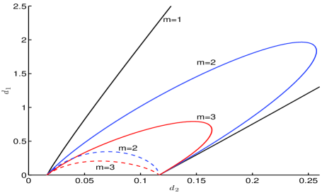
Figure 2: Hopf bifurcation boundaries for the synchronous (solid curve) and asynchronous (dashed curve) modes for the Sel’kov model for different numbers $m$ of cells in the $d_{1}$ versus $d_{2}$ parameter plane. The synchronous mode for $m=1$ is unstable between the two black lines. For $m=2$ and $m=3$ the synchronous mode is unstable in the horseshoe-shaped region bounded by the blue and red solid curves, respectively. Inside the dotted regions for $m=2$ and $m=3$ the asynchronous mode is unstable. For the asynchronous mode, the boundary of these regions is given parametrically by (4.20). The parameters used are $\mu=2$, $\alpha=0.9$, $\epsilon_{0}=0.15$, $\tau=1$, $D_{0}=1$, and $|\Omega|=10$.

We now discuss qualitative aspects of the Hopf bifurcation boundaries for both synchronous and asynchronous modes for various choices of $m$ as seen in Fig. 2. For $m=1$, we need only consider the synchronous instability. The Hopf bifurcation boundary is given by the two black lines, and the region with unstable oscillatory dynamics is located between these two lines. For $m=2$, inside the region bounded by the blue solid curve, the synchronous mode is unstable and under the blue dashed curve, the asynchronous mode is unstable. Similar notation applies to the case with $m=3$, where the Hopf bifurcation boundaries for synchronous/asynchronous mode are denoted by red solid/dashed curves.

One key qualitative feature we can observe from Fig. 2, for the parameter set used, is that the oscillatory region for a larger value of $m$ lies completely within the unstable region for smaller $m$ for both the synchronous and asynchronous modes. This suggests that if a coupled system with $m_{1}$ cells is unstable to synchronous perturbations, then a system with $m_{2}<m_{1}$ cells will also be unstable to such perturbations. However, if a two-cell system is unstable, it is possible that a system with three cells, with the same parameter set, can be stable. Finally, we observe qualitatively that the Hopf bifurcation boundary of the asynchronous mode always lies between that of the synchronous mode. This suggests that as we vary $d_{1}$ and $d_{2}$ from a stable parameter region into an unstable parameter region, we will always first trigger a synchronous oscillatory instability rather than an asynchronous instability. It is an open problem to show that these qualitative observations still hold for a wide range of other parameter sets.

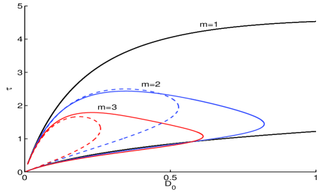
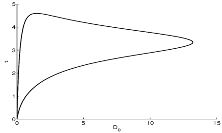
Figure 3: Left panel: Hopf bifurcation boundaries for the synchronous (solid curves) and asynchronous (dashed curves) modes for the Sel’kov model with different numbers $m$ of cells in the $\tau$ versus $D_{0}$ plane. The synchronous mode for $m=1$ is unstable only inside the region bounded by the two black solid curves. Similarly, in the lobe formed by the blue solid and red solid curves the synchronous mode is unstable for $m=2$ (blue) and $m=3$ (red), respectively. In the region enclosed by the blue (red) dashed curve, the asynchronous mode is unstable for $m=2$ ($m=3$). Right panel: Hopf bifurcation boundaries for the synchronous mode with $m=1$ shown in a larger region of the $\tau$ versus $D_{0}$ plane, showing that the instability lobe is a bounded region. Parameters used are $\mu=2$, $\alpha=0.9$, $\epsilon_{0}=0.15$, $d_{1}=0.5$, $d_{2}=0.2$ and $|\Omega|=10$.

Next, we show the region where oscillatory instabilities can occur in the $\tau$ versus $D_{0}$ parameter plane for the synchronous and asynchronous modes. We fix the Sel’kov parameter values as $\mu=2$, $\alpha=0.9$, and $\epsilon_{0}=0.15$, so that the uncoupled intracelluar kinetics has a stable steady-state. We then take $d_{1}=0.5$, $d_{2}=0.2$, and $|\Omega|=10$. For this parameter set, we solve the Hopf bifurcation conditions (4.10) by a root finder. In this way, in the left panel of Fig. 3 we plot the Hopf bifurcation boundaries for the synchronous mode in the $\tau$ versus $D_{0}$ plane for $m=1,2,3$. Similarly, upon using (4.14), in the left panel of Fig. 3 we also plot the Hopf bifurcation boundaries for the asynchronous mode. In the right panel of Fig. 3, where we plot in a larger region of the $\tau$ versus $D$ plane, we show that the instability lobe for the $m=1$ case is indeed closed. We observe for $m=2$ and $m=3$ that, for this parameter set, the lobes of instability for the asynchronous mode are almost entirely contained within the lobes of instability for the synchronous mode.

Finally, we consider the effect of changing $d_{1}$ and $d_{2}$ to $d_{1}=0.1$ and $d_{2}=0.2$, while fixing the Sel’kov parameters as $\mu=2$, $\alpha=0.9$, and $\epsilon_{0}=0.15$, and keeping $|\Omega|=10$. In Fig. 4 we plot the Hopf bifurcation curve for the synchronous mode when $m=1$, computed using (4.10), in the $\tau$ versus $D_{0}$ plane. We observe that there is no longer any closed lobe of instability. In this figure we also show the two Hopf bifurcation values that correspond to taking the limit $D_{0}\gg 1$. These latter values are Hopf bifurcation points for the linearization of the ODE system (5.16) around its steady-state value. This ODE system (5.16), derived in §5, describes large-scale cell-bulk dynamics in the regime $D\gg{\mathcal{O}}(\nu^{-1})$.

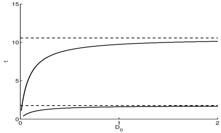
Figure 4: Hopf bifurcation boundaries for the synchronous mode for the Sel’kov model with $m=1$ in the $\tau$ versus $D_{0}$ plane when $d_{1}=0.1$ and $d_{2}=0.2$. The other parameters are the same as in Fig. 3. Inside the region bounded by the two black solid curves, which were computed using (4.10), the synchronous mode is unstable. The instability region is no longer a closed lobe as in Fig. 3. The dashed lines represent the two Hopf bifurcation points that are obtained by using the bifurcation software [5] on the steady-state problem for the ODE system (5.16). As $D_{0}$ increases, the Hopf bifurcation thresholds in $\tau$ gradually approach those obtained from the large $D$ approximation.

4.2.2 Local Kinetics Described by a Fitzhugh-Nagumo Type System

Next, for the cell kinetics we take the Fitzhugh-Nagumo (FN) nonlinearities, taken from [7], given by

$$F(v,w)=\epsilon_{0}(wz-v)\,,\qquad G(v,w)=w-q(w-2)^{3}+4-v\,,$$ (4.21)

where the parameters satisfy $\epsilon_{0}>0$, $q>0$, and $z>1$.

Upon substituting (4.21) into (4.6) we calculate that the steady-state solution $w_{e}>0$ is given by the unique real positive root of the cubic ${\mathcal{C}}(w)=0$ given by

$${\mathcal{C}}(w)\equiv qw^{3}-6qw^{2}+w\left(12q-1+\Lambda\right)-(8q+4)\,,\qquad\mbox{where}\qquad\Lambda\equiv\frac{\epsilon_{0}z}{\left[\epsilon_{0}+{2\pi D_{0}\beta/\tau}\right]}\,,$$ (4.22)

where $\beta$ is defined in (4.16). The uniqueness of the positive root of this cubic for any $\Lambda>0$ was proved previously in §2 of [9]. In terms of the solution $w_{e}>0$ to the cubic equation, we calculate $v_{e}=\Lambda w_{e}$ and $S_{0c}=-\beta\Lambda w_{e}$.

As needed below, we first calculate the partial derivatives of $F$ and $G$ at the steady-state solution as

$$F_{v}^{e}=-\epsilon_{0}\,,\qquad F_{w}^{e}=\epsilon_{0}z\,,\qquad G_{v}^{e}=-1\,,\qquad G_{w}^{e}=1-3q(w_{e}-2)^{2}\,,$$ (4.23a)

which yields

$$\mbox{det}(J)=\epsilon_{0}\left[z-1+3q(w_{e}-2)^{2}\right]>0\,,\qquad\mbox{tr}(J)=-\epsilon_{0}+1-3q(w_{e}-2)^{2}\,.$$ (4.23b)

To determine conditions for which the synchronous mode has a Hopf bifurcation we first substitute (4.23a) into (4.8b). The Hopf bifurcation boundary is then found by numerically computing the roots of (4.10). Similarly, to study instabilities associated with the asynchronous oscillatory mode we substitute (4.23a) into (4.12) to obtain that

$$\gamma=\tau\left[-\epsilon_{0}+1-3q(w_{e}-2)^{2}\right]\,,$$ (4.24a)

which yields the Hopf bifurcation boundary, provided that

$$\det(J)-\frac{\gamma}{\tau}G_{w}^{e}=-G_{v}^{e}F_{w}^{e}-(G_{w}^{e})^{2}=-G_{v}^{e}F_{w}^{e}-(G_{w}^{e})^{2}=\epsilon_{0}z-\left[1-3q(w_{e}-2)^{2}\right]^{2}>0\,,$$ (4.24b)

where $w_{e}$ is the positive root of the cubic (4.22). As was done for the Sel’kov model in §4.2.1, the Hopf bifurcation boundary for the asynchronous mode in the $d_{1}$ versus $d_{2}$ parameter plane can be parametrized as in (4.20a) where $a_{11}$, $a_{12}$, $a_{22}$, and $a_{21}$, are now defined in terms of the parameter $w_{e}>0$ by

$$a_{11}\equiv 1+\frac{2\pi mD_{0}}{|\Omega|}\,,\qquad a_{12}\equiv-\frac{1}{\beta(w_{e})}\,,\qquad a_{21}\equiv 1\,,\qquad a_{22}\equiv-\frac{2\pi D_{0}}{\gamma(w_{e})}\,,$$ (4.25a)

where

$$\beta(w_{e})\equiv\frac{\epsilon_{0}\tau}{2\pi D_{0}}\left(\frac{z}{\Lambda(w_{e})}-1\right)\,,\quad\mbox{with}\quad\Lambda(w_{e})\equiv-\frac{q(w_{e}-2)^{3}}{w_{e}}+1+\frac{4}{w_{e}}\,;\quad\gamma(w_{e})\equiv\tau\left[-\epsilon_{0}+1-3q(w_{e}-2)^{2}\right]\,.$$ (4.25b)

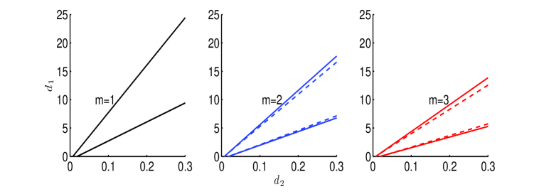
Figure 5: Hopf bifurcation boundaries for the synchronous (solid curve) and asynchronous (dashed curve) modes for the FN system (4.21) with various number $m$ of cells in the $d_{1}$ versus $d_{2}$ parameter plane. Between the solid lines the synchronous mode is unstable, whereas between the dashed lines the asynchronous mode is unstable. Notice that the region of instability for the asynchronous mode is contained within the instability region for the synchronous mode. Parameters used are $z=3.5$, $q=5$, $\epsilon_{0}=0.5$, $\tau=1$, $D_{0}=1$, and $|\Omega|=10$.

By varying $w_{e}>0$ and retaining only the portion of the curve for which $d_{1}>0$ and $d_{2}>0$, and ensuring that the constraint (4.24b) holds, we obtain a parametric form for the Hopf bifurcation boundary for the asynchronous mode in the $d_{1}$ versus $d_{2}$ parameter plane. For $m=2$ and $m=3$, these are the dashed curves shown in Fig. 5.

In this way, in Fig. 5 we plot the Hopf bifurcation boundaries for the synchronous mode (solid curves) and asynchronous mode (dashed curves) for various values of $m$ for the parameter set $z=3.5$, $q=5$, $\epsilon_{0}=0.5$, $\tau=1$, $D_{0}=1$, and $|\Omega|=10$. As compared to Fig. 2, we notice that the unstable regions for both modes are not only shrinking but also the boundaries shift as the number of cells increases. This feature does not appear in the previous Sel’kov model.

Next, in Fig. 6 we show the region where oscillatory instabilities occur for either synchronous or asynchronous modes for $m=1,2,3$ in the $\tau$ versus $D_{0}$ plane. These Hopf bifurcation boundaries are computed by finding roots of either (4.10) or (4.24) for various values of $D_{0}$. The other parameter values are the same as those used for Fig. 5 except $d_{1}=10$ and $d_{2}=0.2$. Inside the region bounded by the solid curves the synchronous mode is unstable, while inside the region bounded by the dashed curves, the asynchronous mode is unstable. Similar to that shown in Fig. 5, the regions of instability are shrinking, at the same time as the Hopf bifurcation boundaries shift, as $m$ increases. For these parameter values of $d_{1}$ and $d_{2}$, the Hopf bifurcation for the synchronous model still occurs for large values of $D_{0}$.

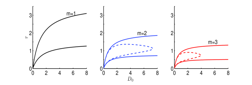
Figure 6: Hopf bifurcation boundaries for the synchronous (solid curves) and asynchronous (dashed curves) modes for the FN system (4.21) with various number $m$ of cells in the $\tau$ versus $D_{0}$ parameter plane. Between the solid lines the synchronous mode is unstable, whereas between the dashed lines the asynchronous mode is unstable. Parameters used are $z=3.5$, $q=5$, $\epsilon_{0}=0.5$, $d_{1}=10$, $d_{2}=0.2$, and $|\Omega|=10$.

5 Finite Domain: Reduction to ODEs for $D\gg{\mathcal{O}}(\nu^{-1})$

In this section we assume that there is one small dynamically active circular cell $\Omega_{\epsilon}$ in the bounded domain $\Omega$ under the assumption that $D\gg{\mathcal{O}}(\nu^{-1})$, with $\nu={-1/\log\epsilon}$. In this limit, in which the bulk region is effectively well-mixed, we now show that we can reduce the dynamics for the coupled cell-bulk model to a system of nonlinear ODEs.

For the case of one cell, the basic model is formulated as

$$\tau U_{t}=D\Delta U-U\,,\qquad\boldsymbol{x}\in\Omega\backslash\Omega_{\epsilon}\,;\qquad\partial_{n}U=0\,,\qquad\boldsymbol{x}\in\partial\Omega\,;\qquad\epsilon D\partial_{n}U=d_{1}U-d_{2}u^{1}\,,\;\;\quad\boldsymbol{x}\in\partial\Omega_{\epsilon}\,,$$ (5.1a)

which is coupled to the intracellular cell dynamics, with $$\boldsymbol{u}=(u_{1},\ldots,u_{n})^{T} \boldsymbol{F}(\boldsymbol{u})$$ and reaction kinetics , by

$$\frac{d\boldsymbol{u}}{dt}=\boldsymbol{F}(\boldsymbol{u})+\frac{\boldsymbol{e}_{1}}{\epsilon\tau}\int_{\partial\Omega_{\epsilon}}(d_{1}U-d_{2}u_{1})\,ds\,,\qquad\mbox{where}\qquad\boldsymbol{e}_{1}\equiv(1,0,\dots,0)^{T}\,.$$ (5.1b)

We will assume that $D\gg 1$, and so in the bulk region we expand

$$U=U_{0}+\frac{1}{D}U_{1}+\cdots\,.$$ (5.2)

Upon substituting this expansion into (5.1a), and noting that $\Omega_{\epsilon}\to\boldsymbol{x}_{0}$ as $\epsilon\to 0$, we obtain to leading order in ${1/D}$ that $\Delta U_{0}=0$ with $\partial_{n}U_{0}=0$ on $\partial\Omega$. As such, we have that $U_{0}=U_{0}(t)$. At next order, we have that $U_{1}$ satisfies

$$\Delta U_{1}=U_{0}+\tau U_{0t},\quad\boldsymbol{x}\in\Omega\backslash\{\boldsymbol{x}_{0}\}\,;\qquad\partial_{\boldsymbol{n}}U_{1}=0,\quad\boldsymbol{x}\in\partial\Omega\,.$$ (5.3)

The formulation of this problem is complete once we determine a matching condition for $U_{1}$ as $\boldsymbol{x}\rightarrow\boldsymbol{x}_{0}$.

To obtain this matching condition, we must consider the inner region defined at ${\mathcal{O}}(\epsilon)$ distances outside the cell. In this inner region we introduce the new variables $\boldsymbol{y}=\epsilon^{-1}(\boldsymbol{x}-\boldsymbol{x}_{0})$ and $\hat{U}(\boldsymbol{y},t)=U(\boldsymbol{x}_{0}+\epsilon\boldsymbol{y},t)$. From (5.1a), we obtain that

$$\tau\hat{U_{t}}=\frac{D}{\epsilon^{2}}\Delta_{\boldsymbol{y}}\hat{U}-\hat{U},\quad\rho=|\boldsymbol{y}|\geq 1\,;\qquad D\frac{\partial\hat{U}}{\partial\rho}=d_{1}\hat{U}-d_{2}u_{1}\,,\quad\mbox{on}\quad\rho=1\,.$$

For $D\gg 1$, we then seek a radially symmetric solution to this inner problem in the form

$$\hat{U}(\rho,t)=\hat{U}_{0}(\rho,t)+\frac{1}{D}\hat{U}_{1}(\rho,t)+\cdots\,.$$ (5.4)

To leading order we obtain $\Delta_{\rho}\hat{U}_{0}=0$ in $\rho\geq 1$, with $\hat{U}_{0\rho}=0$ on $\rho=1$, subject to the matching condition to the bulk that $\hat{U}_{0}\to U_{0}$ as $\rho\to\infty$. We conclude that $\hat{U}_{0}=U_{0}$. At next order, the problem for $\hat{U}_{1}$ is

$$\Delta_{\rho}\hat{U}_{1}=0\,,\qquad\rho\geq 1\,;\qquad\frac{\partial\hat{U}_{1}}{\partial\rho}=d_{1}U_{0}-d_{2}u_{1}\,,\qquad\rho=1\,.$$ (5.5)

Allowing for logarithmic growth at infinity, the solution to this problem is

$$\hat{U}_{1}=(d_{1}U_{0}-d_{2}u_{1})\log\rho+C\,,$$ (5.6)

where $C$ is a constant to be found. Then, by writing (5.6) in outer variables, and recalling (5.4), we obtain that the far-field behavior of the inner expansion is

$$\hat{U}\sim U_{0}+\frac{1}{D}\left[\left(d_{1}U_{0}-d_{2}u_{1}\right)\log|\boldsymbol{x}-\boldsymbol{x}_{0}|+\frac{1}{\nu}\left(d_{1}U_{0}-d_{2}u_{1}\right)+C\right]+\cdots\,.$$ (5.7)

From (5.7) we observe that the term proportional to ${1/D}$ is smaller than the first term provided that $D\gg O(\nu^{-1})$. This specifies the asymptotic range of $D$ for which our analysis will hold. From asymptotic matching of the bulk and inner solutions, the far-field behavior of the inner solution (5.7) provides the required singular behavior as $\boldsymbol{x}\to\boldsymbol{x}_{0}$ for the outer bulk solution. In this way, we find from (5.7) and (5.2) that $U_{1}$ satisfies (5.3) subject to the singular behavior

$$U_{1}\sim\left(d_{1}U_{0}-d_{2}u_{1}\right)\log|\boldsymbol{x}-\boldsymbol{x}_{0}|\,,\quad\mbox{as}\quad\boldsymbol{x}\to\boldsymbol{x}_{0}\,.$$ (5.8)

Then, (5.3) together with (5.8) determines $U_{1}$ uniquely. Finally, in terms of this solution, we identify that the constant $C$ in (5.7) and (5.6) is obtained from

$$\lim_{\boldsymbol{x}\to\boldsymbol{x}_{0}}\left[U_{1}-\left(d_{1}U_{0}-d_{2}u_{1}\right)\log|\boldsymbol{x}-\boldsymbol{x}_{0}|\right]=\nu^{-1}\left(d_{1}U_{0}-d_{2}u_{1}\right)+C\,.$$ (5.9)

We now carry out the details of the analysis. We can write the problem (5.3) and (5.8) for $U_{1}$ as

$$\Delta U_{1}=U_{0}+\tau U_{0t}+2\pi\left(d_{1}U_{0}-d_{2}u_{1}\right)\delta(\boldsymbol{x}-\boldsymbol{x}_{0})\,,\qquad\boldsymbol{x}\in\Omega\,;\qquad\partial_{n}U_{1}=0,\quad\boldsymbol{x}\in\partial\Omega\,.$$ (5.10)

By the divergence theorem, this problem has a solution only if $\left(U_{0}+\tau U_{0t}\right)|\Omega|=-2\pi(d_{1}U_{0}-d_{2}u_{1})$. This leads to the following ODE for the leading-order bulk solution $U_{0}(t)$:

$$U_{0}^{\prime}=-\frac{1}{\tau}\left(1+\frac{2\pi d_{1}}{|\Omega|}\right)U_{0}+\frac{2\pi d_{2}}{\tau|\Omega|}u_{1}\,.$$ (5.11)

Without loss of generality we impose $\int_{\Omega}U_{1}\,d\boldsymbol{x}=0$ so that $U_{0}$ is the spatial average of $U$. Then, the solution to (5.10) is

$$U_{1}=-2\pi\left(d_{1}U_{0}-d_{2}u_{1}\right)G_{0}(\boldsymbol{x};\boldsymbol{x}_{0})\,,$$ (5.12)

where $G_{0}(\boldsymbol{x};\boldsymbol{x}_{0})$ is the Neumann Green’s function defined by (3.5). We then expand (5.12) as $\boldsymbol{x}\to\boldsymbol{x}_{0}$, and use (5.9) to identify $C$ in terms of the regular part $R_{0}$ of the Neumann Green’s function, defined in (3.5), as

$$C=-\left(d_{1}U_{0}-d_{2}u_{1}\right)\left(\nu^{-1}+2\pi R_{0}\right)\,.$$ (5.13)

In summary, by using (5.4), (5.6), and (5.13), the two-term inner expansion near the cell is given by

$$\hat{U}\sim U_{0}+\frac{1}{D}\left(d_{1}U_{0}-d_{2}u_{1}\right)\left(\log\rho-\frac{1}{\nu}-2\pi R_{0}\right)+\cdots\,.$$ (5.14)

From (5.2) and (5.12), the two-term expansion for the outer bulk solution, in terms of $U_{0}(t)$ satisfying the ODE (5.11), is

$$U\sim U_{0}-\frac{2\pi}{D}\left(d_{1}U_{0}-d_{2}u_{1}\right)G_{0}(\boldsymbol{x};\boldsymbol{x}_{0})\,.$$ (5.15)

The final step in the analysis is to use (5.1b) to derive the dynamics inside the cell. We readily calculate that

$$\frac{1}{\epsilon\tau}\int_{\partial\Omega_{\epsilon}}\left(d_{1}U-d_{2}u_{1}\right)\,ds\sim\frac{2\pi}{\tau}\left(d_{1}U_{0}-d_{2}u_{1}\right)\,,$$

which determines the dynamics inside the cell from (5.1b).

This leads to our main result that, for $D\gg{\mathcal{O}}(\nu^{-1})$, the coupled PDE model (5.1) reduces to the study of the coupled (n+1) dimensional ODE system for the leading-order average bulk concentration $U_{0}(t)$ and cell dynamics $\boldsymbol{u}$ given by

$$U_{0}^{\prime}=-\frac{1}{\tau}\left(1+\frac{2\pi d_{1}}{|\Omega|}\right)U_{0}+\frac{2\pi d_{2}}{\tau|\Omega|}u_{1}\,,\qquad\boldsymbol{u}^{\prime}=\boldsymbol{F}(\boldsymbol{u})+\frac{2\pi}{\tau}\left[d_{1}U_{0}-d_{2}u_{1}\right]\boldsymbol{e}_{1}\,.$$ (5.16)

Before studying (5.16) for some specific reaction kinetics, we first examine conditions for the existence of steady-state solutions for (5.16) and we derive the spectral problem characterizing the linear stability of these steady-states.

A steady-state solution $U_{0e}$ and $\boldsymbol{u}_{e}$ of (5.16), if it exists, is a solution to the nonlinear algebraic system

$$\boldsymbol{F}(\boldsymbol{u}_{e})+\frac{2\pi}{\tau}\left(d_{1}U_{0e}-d_{2}\boldsymbol{u}_{1e}\right)\boldsymbol{e}_{1}=0\,,\qquad rU_{0e}=su_{1e}\,,\qquad\mbox{where}\qquad r\equiv 1+\frac{2\pi d_{1}}{|\Omega|}\,,\qquad s\equiv\frac{2\pi d_{2}}{|\Omega|}\,.$$ (5.17)

To examine the linearized stability of such a steady-state, we substitute $U_{0}=U_{0e}+e^{\lambda t}\eta$ and $\boldsymbol{u}=\boldsymbol{u}_{e}+e^{\lambda t}\boldsymbol{\phi}$ into (5.16) and linearize. This yields that $\eta$ and $\boldsymbol{\phi}$ satisfy

$$\lambda\boldsymbol{\phi}=J\boldsymbol{\phi}+\frac{2\pi}{\tau}\left(d_{1}\eta-d_{2}\phi_{1}\right)\boldsymbol{e}_{1}\,,\qquad\tau\lambda\eta=-r\eta+s\phi_{1}\,,$$

where $J$ is the Jacobian of $\boldsymbol{F}$ evaluated at the steady-state $\boldsymbol{u}=\boldsymbol{u}_{e}$. Upon solving the second equation for $\eta$, and substituting the resulting expression into the first equation, we readily derive the homogeneous linear system

$$\left[(\lambda I-J)-\mu{\mathcal{E}}_{1}\right]\boldsymbol{\phi}=0\,,\qquad\mbox{where}\qquad\mu\equiv\frac{2\pi}{\tau}\left(\frac{d_{1}s}{\tau\lambda+r}-d_{2}\right)\,,\qquad{\mathcal{E}}_{1}\equiv\boldsymbol{e}_{1}\boldsymbol{e}_{1}^{T}\,.$$ (5.18)

By using the matrix determinant lemma we conclude that $\lambda$ is an eigenvalue of the linearization if and only if $\lambda$ satisfies $\boldsymbol{e}_{1}^{T}\left(\lambda I-J\right)^{-1}\boldsymbol{e}_{1}={1/\mu}$, where $\mu$ is defined in (5.18). From this expression, and by using $d_{1}s-d_{2}r=-d_{2}$ as obtained from (5.17), we conclude that $\lambda$ must be a root of ${\mathcal{Q}}(\lambda)=0$, defined by

$${\mathcal{Q}}(\lambda)\equiv\frac{{\tau}(r+\tau\lambda)}{2\pi d_{2}\left(1+\tau\lambda\right)}+\frac{M_{11}}{\det(\lambda I-J)}\,,$$ (5.19)

where $r$ is defined in (5.17). Here $M_{11}$ is the cofactor of the element in the first row and first column of $\lambda I-J$.

Next, we show that (5.19), which characterizes the stability of a steady-state solution of the ODE dynamics (5.16), can also be derived by taking the limit $D_{0}\gg 1$ in the stability results obtained in (3.16) of §3 for the $D={\mathcal{O}}(\nu^{-1})$ regime where we set $D={D_{0}/\nu}$. Recall from the analysis in §3 for $D={D_{0}/\nu}$, that when $m=1$ only the synchronous mode can occur, and that the linearized eigenvalue satisfies (3.17). By formally letting $D_{0}\to\infty$ in (3.17) we readily recover (5.19).

5.1 Large D Theory: Analysis of Reduced Dynamics

We now give some examples of our stability theory. We first consider the case where there is exactly one dynamical species in the cell so that $n=1$. From (5.17) with $n=1$ we obtain that the steady-state $u_{e}$ is any solution of

$$F(u_{e})-\frac{2\pi d_{2}}{\tau}\left[1+\frac{2\pi d_{1}}{|\Omega|}\right]^{-1}u_{e}=0\,,\qquad U_{0e}=\frac{2\pi d_{2}}{|\Omega|}\left[1+\frac{2\pi d_{1}}{|\Omega|}\right]^{-1}u_{e}\,.$$ (5.20)

In the stability criterion (5.19) we set $M_{11}=1$ and $\det(\lambda I-J)=\lambda-F_{u}^{e}$, where $F_{u}^{e}\equiv{dF/du}|_{u=u_{e}}$, to conclude that the stability of this steady-state is determined by the roots of the quadratic

$$\lambda^{2}-\lambda p_{1}+p_{2}=0\,,$$ (5.21a)

where $$p_{1} p_{2}$$ and are defined by

$$p_{1}=-\frac{1}{\tau}\left(1+\frac{2\pi d_{1}}{|\Omega|}\right)+F_{u}^{e}-\frac{2\pi d_{2}}{\tau}\,,\qquad p_{2}=-\frac{F_{u}^{e}}{\tau}\left(1+\frac{2\pi d_{1}}{|\Omega|}\right)+\frac{2\pi d_{2}}{\tau^{2}}\,.$$ (5.21b)

We now establish the following result based on (5.21).

Principal Result 5.1

Let $n=1$. Then, no steady-state solution of (5.16) can undergo a Hopf bifurcation. Moreover, if

$$\qquad F_{u}^{e}<F_{\textrm{th}}\equiv\frac{2\pi d_{2}}{\tau}\left[1+\frac{2\pi d_{1}}{|\Omega|}\right]^{-1}\,,$$ (5.22)

then $\mbox{Re}(\lambda)<0$, and so the steady-state is linearly stable. If $F_{u}^{e}>F_{\textrm{th}}$, the linearization has exactly one positive eigenvalue.

Proof 5.1.

We first prove that no Hopf bifurcations are possible for the steady-state. From (5.21a) it is clear that there exists a Hopf bifurcation if and only if $p_{1}=0$ and $p_{2}>0$ in (5.21b). Upon setting $p_{1}=0$, we get $F_{u}^{e}=2\pi d_{2}{\tau^{-1}}+\tau^{-1}\left(1+{2\pi d_{1}/|\Omega|}\right)$. Upon substituting this expression into (5.21b) for $p_{2}$, we get that

$$p_{2}=-\frac{1}{\tau}\left[\frac{4\pi^{2}d_{2}^{2}}{{\tau}|\Omega|}+\frac{1}{\tau}\left(1+\frac{2\pi d_{1}}{|\Omega|}\right)\left(1+\frac{2\pi d_{2}}{|\Omega|}\right)\right]<0\,.$$

Since $p_{2}<0$ whenever $p_{1}=0$, we conclude that no Hopf bifurcations for the steady-state are possible.

The second result follows by showing that $p_{1}<0$ and $p_{2}>0$ when $F_{u}^{e}<F_{\textrm{th}}$. From (5.21b), $p_{1}<0$ and $p_{2}>0$ when

$$\frac{2\pi d_{2}}{\tau}-F_{u}^{e}+\frac{1}{\tau}\left(1+\frac{2\pi d_{1}}{|\Omega|}\right)>0\,,\qquad\frac{2\pi d_{2}}{\tau}-F_{u}^{e}-\frac{2\pi d_{1}}{|\Omega|}F_{u}^{e}>0\,.$$ (5.23)

These two inequalities hold simultaneously only when the second relation is satisfied. This yields that when (5.22) holds, we have $\mbox{Re}(\lambda)<0$. Finally, when $F_{u}^{e}>F_{\textrm{th}}$, we have $p_{2}<0$, and so there is a unique positive eigenvalue.

This result shows that with cell-bulk coupling the steady-state of the ODE (5.16) can be linearly stable even when the reaction kinetics is self-activating in the sense that $F_{u}^{e}>0$. Moreover, we observe that as $\tau$ increases, corresponding to when the intracellular kinetics has increasingly faster dynamics than the time scale for bulk decay, then the stability threshold $F_{\textrm{th}}$ decreases. Therefore, for fast cell dynamics there is a smaller parameter range where self-activation of the intracelluar dynamics can occur while still maintaining stability of the steady-state to the coupled system.

Next, we let $n=2$ where $\boldsymbol{F}(\boldsymbol{u})=(F(u_{1},u_{2}),G(u_{1},u_{2}))^{T}$. Then, the steady-state of the ODEs (5.16) satisfies

$$F(u_{1e},u_{2e})-\frac{2\pi d_{2}}{r\tau}u_{1e}=0\,,\qquad G(u_{1e},u_{2e})=0\,,\qquad U_{0e}=\frac{s}{r}u_{1e}\,,$$ (5.24)

where $r$ and $s$ are defined in (5.17). We then observe that the roots of ${\mathcal{Q}}(\lambda)=0$ in (5.19) are roots to a cubic polynomial in $\lambda$. Since $M_{11}=\lambda-G_{u_{2}}^{e}$, $\det(\lambda I-J)=\lambda^{2}-\mbox{tr}(J)\lambda+\det J$, where

$$\mbox{tr}(J)=F_{u_{1}}^{e}+G_{u_{2}}^{e}\,,\qquad\det J=F_{u_{1}}^{e}G_{u_{2}}^{e}-F_{u_{2}}^{e}G_{u_{1}}^{e}\,,$$ (5.25)

and $F_{v}^{e}$, $G_{v}^{e}$ are partial derivatives of $F$ or $G$ with respect to $v\in(u_{1},u_{2})$ evaluated at the steady-state, we conclude that the linear stability of the steady-state is characterized by the roots of the cubic

$$\lambda^{3}+p_{1}\lambda^{2}+p_{2}\lambda+p_{3}=0\,,$$ (5.26a)

where $$p_{1} p_{2} p_{3}$$, and are defined as

$$\begin{split}p_{1}&\equiv\frac{2\pi d_{2}}{\tau}+\frac{1}{\tau}\left(1+\frac{2\pi d_{1}}{|\Omega|}\right)-\mbox{tr}(J)\,,\qquad p_{3}\equiv\frac{1}{\tau}\left(\left(1+\frac{2\pi d_{1}}{|\Omega|}\right)\det J-\frac{2\pi d_{2}}{\tau}G_{u2}^{e}\right)\,,\\ p_{2}&\equiv\det J-\frac{2\pi d_{2}}{\tau}G_{u_{2}}^{e}+\frac{1}{\tau}\left(\frac{2\pi d_{2}}{\tau}-\left(1+\frac{2\pi d_{1}}{|\Omega|}\right)\mbox{tr}(J)\right)\,.\end{split}$$ (5.26b)

By taking $m=1$ and letting $D_{0}\rightarrow\infty$ in (4.8b), it is readily verified that the expressions above for $p_{i}$, for $i=1,2,3$, agree exactly with those in (4.8b). Then, by satisfying the Routh-Hurwitz conditions (4.10), we can plot the Hopf bifurcation boundaries in different parameter planes.

5.1.1 Example: One Cell with Sel’kov Dynamics

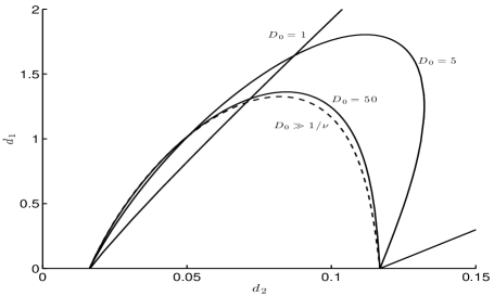
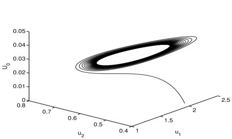
Figure 7: Left panel: Comparison of the Hopf bifurcation boundaries for the synchronous mode for the Sel’kov model (4.15) in the $d_{1}$ versus $d_{2}$ plane with $D_{0}=1,\ 5,\ 50$ (solid), as obtained from (4.8), and the large $D$ approximation (dashed), as obtained from (5.26). Between the outer two black curves, the synchronous mode is unstable for $D_{0}=1$. In the region bounded by the solid or dashed curve this mode is unstable. As $D_{0}$ increases, the Hopf boundaries from (4.8) gradually approach the one given in from the large $D$ approximation. Right panel: Numerical results for the ODE system (5.16) showing sustained oscillations. In the left and right panels we fixed $\mu=2$, $\alpha=0.9$, $\epsilon_{0}=0.15$, $\tau=1$, and $|\Omega|=10$. In the right panel we took $d_{1}=0.8$ and $d_{2}=0.05$ for which the steady-state solution of the ODEs (5.16) is unstable.

When the intracellular kinetics is described by the Sel’kov model, where $F$ and $G$ are given in (4.15), we obtain from (5.24) that the steady-state solution of the ODE dynamics is

$$u_{1}^{e}=\frac{r\mu}{\left[r+{2\pi d_{2}/\tau}\right]}\,,\qquad u_{2}^{e}=\frac{\mu}{\alpha+(u_{1}^{e})^{2}}\,,\qquad U_{0e}=\frac{s\mu}{r+{2\pi d_{2}/\tau}}\,,$$ (5.27)

where $r$ and $s$ are defined in (5.17). The partial derivatives of $F$ and $G$ can be calculated as in (4.17a).

In the left panel of Fig. 7 we plot the Hopf bifurcation boundary in the $d_{1}$ versus $d_{2}$ plane associated with linearizing the ODEs (5.16) about this steady-state solution. This curve was obtained by setting $p_{1}p_{2}=p_{3}$ with $p_{1}>0$ and $p_{3}>0$ in (5.26). In this figure we also plot the Hopf bifurcation boundary for different values of $D_{0}$, with ${D=D_{0}/\nu}$, as obtained from our stability formulation (4.8) of §4 for the $D={\mathcal{O}}(\nu^{-1})$ regime. We observe from this figure that the stability boundary with $D_{0}=50$ closely approximates that obtained from (5.26), which corresponds to the $D_{0}\to\infty$ limit of (4.8).

We emphasize that since in the distinguished limit $D\gg{\mathcal{O}}(\nu^{-1})$ we can approximate the original coupled PDE system (5.1) by the system (5.16) of ODEs, the study of large-scale time dynamics far from the steady-state becomes tractable. In the right panel of Fig. 7, we plot the numerical solution to (5.16) with Sel’kov dynamics (4.15), where the initial condition is $u_{1}(0)=0.01$, $u_{2}(0)=0.2$, and $U_{0}(0)=0.5$. We observe that by choosing $d_{1}$ and $d_{2}$ inside the region bounded by the dashed curve in the left panel of Fig. 7, where the steady-state is unstable, the full ODE system (5.16) exhibits a stable periodic orbit, indicating a limit cycle behavior.

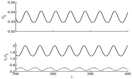
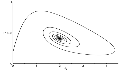
Figure 8: Left panel: $u_{1}$, $u_{2}$ and $U_{0}$ versus $t$ showing sustained oscillatory dynamics. Parameters are $\mu=2$, $\alpha=0.9$, $\epsilon_{0}=0.15$, $\tau=1$, $|\Omega|=10$, $d_{1}=0.8$ and $d_{2}=0.05$. Right panel: $u_{2}$ versus $u_{1}$ when the local kinetics is decoupled from the bulk, showing decaying oscillations towards the stable steady-state solution $u_{1}=\mu$ and $u_{2}=\mu/(\alpha+u_{1}^{2})$. Initial values are $u_{1}(0)=0.01$ and $u_{2}(0)=0.2$. The parameter values of $\mu$, $\epsilon_{0}$ and $\alpha$ are the same as in the left panel.

In addition, in the left panel of Fig. 8 we plot the time evolution of $u_{1}$, $u_{2}$ and $U_{0}$, showing clearly the sustained periodic oscillations. For comparison, fixing the same parameter set for the Sel’kov kinetics (4.15), in the right panel of Fig. 8 we plot the phase plane of $u_{2}$ versus $u_{1}$ when there is no coupling between the local kinetics and the bulk. We now observe that without this cell-bulk coupling the Sel’kov model (4.15) exhibits transient decaying oscillatory dynamics, with a spiral behavior in the phase-plane towards the linearly stable steady-state.

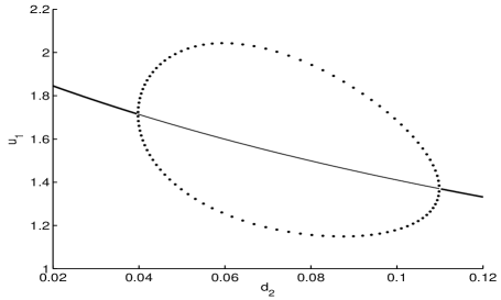
Figure 9: Global bifurcation diagram of $u_{1}$ with respect to $d_{2}$ at a fixed $d_{1}=0.8$ as computed using XPPAUT [5] from the ODE system (5.16) for the Sel’kov kinetics (4.15). The thick/thin solid line represents stable/unstable steady-state solutions of $u_{1}$, while the solid dots indicate a stable periodic solution branch. The parameters used are $\mu=2$, $\alpha=0.9$, $\epsilon_{0}=0.15$, $\tau=1$, and $|\Omega|=10$.

Finally, we use the numerical bifurcation software XPPAUT [5] to confirm the existence of a stable large amplitude periodic solution to (5.16) with Sel’kov kinetics when $d_{1}$ and $d_{2}$ are in the unstable region of the left panel of Fig. 7. In Fig. 9 we plot a global bifurcation diagram of $u_{1}$ versus $d_{2}$ for $d_{1}=0.8$, corresponding to taking a horizontal slice at fixed $d_{2}=0.8$ through the stability boundaries in the $d_{2}$ versus $d_{1}$ plane shown in Fig. 7. The two computed Hopf bifurcation points at $d_{2}\approx 0.0398$ and $d_{1}=0.1098$ agree with the theoretically predicted values in Fig. 7.

5.1.2 Example: One Cell with Fitzhugh-Nagumo Dynamics

Finally, we apply our large $D$ theory to the case where the intracellular dynamics is governed by the FN kinetics (4.21). From (5.24) we obtain that the steady-state solution of the ODEs (5.16) with the kinetics (4.21) is

$$u_{1}^{e}=\Lambda u_{2}^{e}\,,\qquad U_{0e}=\frac{su_{1}^{e}}{r}\,,\qquad\mbox{where}\qquad\Lambda\equiv\frac{\epsilon_{0}zr}{\left[\epsilon_{0}r+{2\pi d_{2}/{\tau}}\right]}\,.$$ (5.28)

Here $r$ and $s$ are defined in (5.17), and $u_{2e}>0$ is the unique root of the cubic (4.22) where $\Lambda$ in (4.22) is now defined in (5.28). The partial derivatives of $F$ and $G$ can be calculated as in (4.23).

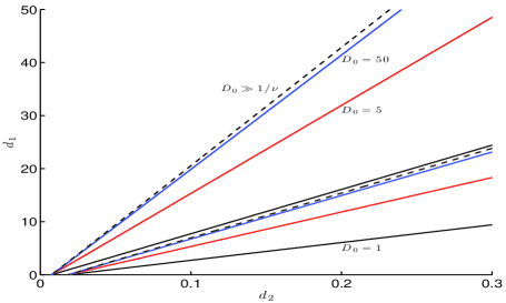
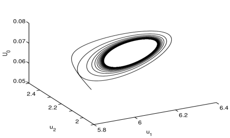
Figure 10: Left panel: Comparison of the Hopf bifurcation boundaries for the synchronous mode with FN kinetics (4.21) in the $d_{1}$ versus $d_{2}$ parameter plane with $D_{0}=1,\ 5,\ 50$ (solid), as obtained from (4.8), and the large $D$ approximation (dashed), as obtained from (5.26). In the wedge-shaped regions bounded by the solid curves the synchronous mode is unstable for the finite values of $D_{0}$. As $D_{0}$ increases, the Hopf boundaries obtained from (4.8) becomes rather close to the dashed one obtained from (5.26) from the large $D$ approximation. Right panel: Numerical simulation for the ODE system (5.16), showing sustained oscillations, with initial conditions $u_{1}(0)=6.0$, $u_{2}(0)=2.3$, and $U_{0}(0)=0.05$. In the left and right panels we fixed $z=3.5$, $q=5$, $\epsilon_{0}=0.5$, $\tau=1$, and $|\Omega|=10$, and in the right panel we took $d_{1}=15.6$ and $d_{2}=0.2$ corresponding to a point where the steady-state solution of the ODEs (5.16) is unstable.

In the left panel of Fig. 10 the dashed curve is the Hopf bifurcation boundary in the $d_{1}$ versus $d_{2}$ plane associated with linearizing the ODEs (5.16) about this steady-state solution. In this figure the Hopf bifurcation boundaries for different values of $D_{0}$, with ${D=D_{0}/\nu}$, are also shown. These latter curves were obtained from our stability formulation (4.8) of §4. Similar to what we found for the Sel’kov model, the stability boundary for $D_{0}=50$ is very close to that for the infinite $D$ result obtained from (5.26). In the right panel of Fig. 10 we plot the numerical solution to (5.16) with FN dynamics (4.21) for the parameter set $d_{1}=15.6$ and $d_{2}=0.2$, which is inside the unstable region bounded by the dashed curves in the left panel of Fig. 10. With the initial condition $u_{1}(0)=6.0$, $u_{2}(0)=2.3$, and $U_{0}(0)=0.05$, the numerical computations of the full ODE system (5.16) again reveal a sustained and stable periodic solution.

Finally, we use XPPAUT [5] on (5.16) to compute a global bifurcation of $u_{1}$ versus $d_{1}$ for fixed $d_{2}=0.2$ for FN kinetics. This plot corresponds to taking a vertical slice at fixed $d_{2}=0.2$ through the stability boundaries in the $d_{1}$ versus $d_{2}$ plane shown in Fig. 10. The two computed Hopf bifurcation points at $d_{1}\approx 15.389$ and $d_{1}=42.842$ agree with the predicted values in Fig. 10. These results confirm the existence of a stable periodic solution branch induced by the cell-bulk coupling.

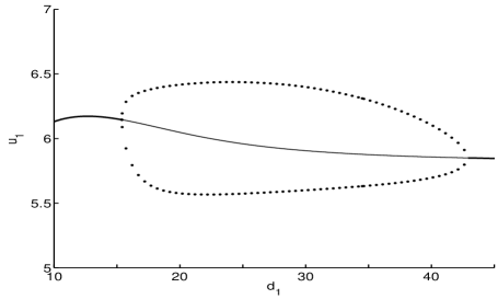
Figure 11: Global bifurcation diagram of $u_{1}$ versus $d_{1}$ when $d_{2}=0.2$, as computed using XPPAUT [5] from the ODE system (5.16) for the FN kinetics (4.21). The thick/thin solid line represents stable/unstable steady-state solutions, while the solid dots indicate a stable periodic solution. The other parameters are $z=3.5$, $q=5$, $\epsilon_{0}=0.5$, $\tau=1$, and $|\Omega|=10$.

6 The Effect of the Spatial Configuration of the Small Cells: The $D={\mathcal{O}}(1)$ Regime

In this section we construct steady-state solutions and study their linear stability properties in the $D={\mathcal{O}}(1)$ regime, where both the number of cells and their spatial distribution in the domain are important factors. For simplicity, we consider a special spatial configuration of the cells inside the unit disk $\Omega$ for which the Green’s matrix ${\mathcal{G}}$ has a cyclic structure. More specifically, on a ring of radius $r_{0}$, with $0<r_{0}<1$, we place $m$ equally-spaced cells whose centers are at

$$\boldsymbol{x}_{j}=r_{0}\left(\cos\left(\frac{2\pi j}{m}\right)\,,\sin\left(\frac{2\pi j}{m}\right)\right)^{T}\,,\qquad\qquad j=1,\ldots,m\,.$$ (6.1)

This ring of cells is concentric with respect to the unit disk $\Omega\equiv\{{\boldsymbol{x}\,|\,|\boldsymbol{x}|\leq 1\,\}}$. We also assume that the intracellular kinetics is the same within each cell, so that $\boldsymbol{F}_{j}=\boldsymbol{F}$ for $j=1,\ldots,m$. A related type of analysis characterizing the stability of localized spot solutions for the Gray-Scott RD model, where localized spots are equally-spaced on a ring concentric with the unit disk, was performed in [3].

For the unit disk, the Green’s function $G(\boldsymbol{x};\boldsymbol{\xi})$ satisfying (2.8) can be written as an infinite sum involving the modified Bessel functions of the first and second kind $I_{n}(z)$ and $K_{n}(z)$, respectively, in the form (see Appendix A.1 of [3])

$$G(\boldsymbol{x};\boldsymbol{\xi})=\frac{\,1}{\,2\pi}K_{0}\left(\theta_{0}|\boldsymbol{x}-\boldsymbol{\xi}|\right)-\frac{\,1}{\,2\pi}\sum^{\infty}_{n=0}\sigma_{n}\cos\left(n(\psi-\psi_{0})\right)\frac{K^{\prime}_{n}(\theta_{0})}{I^{\prime}_{n}(\theta_{0})}I_{n}\left(\theta_{0}r\right)I_{n}\left(\theta_{0}r_{0}\right)\,;\quad\sigma_{0}=1\,,\quad\sigma_{n}=2\,,\,\,\,n\geq 1\,.$$ (6.2)

Here $\theta_{0}\equiv D^{-1/2}$, $\boldsymbol{x}=re^{i\psi}$, $\boldsymbol{\xi}=r_{0}e^{i\psi_{0}}$, and $|\boldsymbol{x}-\boldsymbol{\xi}|=\sqrt{r^{2}+r_{0}^{2}-2rr_{0}\cos(\psi-\psi_{0})}$. By using the local behavior $K_{0}(z)\sim-\log{z}+\log{2}-\gamma_{e}+o(1)$ as $z\to 0^{+}$, where $\gamma_{e}$ is Euler’s constant, we can extract the regular part $R$ of $G(\boldsymbol{x};\boldsymbol{\xi})$ as $\boldsymbol{x}\to\boldsymbol{\xi}$, as identified in (2.8b), as

$$R=\frac{1}{2\pi}\left(\log{2}-\gamma_{e}+\frac{1}{2}\log{D}\right)-\frac{\,1}{\,2\pi}\sum^{\infty}_{n=0}\sigma_{n}\frac{K^{\prime}_{n}(\theta_{0})}{I^{\prime}_{n}(\theta_{0})}\left[I_{n}\left(\theta_{0}r_{0}\right)\right]^{2}\,.$$ (6.3)

For this spatial configuration of cells, the Green’s matrix ${\mathcal{G}}$ is obtained by a cyclic permutation of its first row vector $\boldsymbol{a}\equiv(a_{1},\ldots,a_{m})^{T}$, which is defined term-wise by

$$a_{1}\equiv R\,;\qquad a_{j}=G_{j1}\equiv G(\boldsymbol{x}_{j};\boldsymbol{x}_{1})\,,\quad j=2,\ldots,m\,.$$ (6.4)

We can numerically evaluate $G_{j1}$ for $j=2,\ldots,m$ and $R$ by using (6.2) and (6.3), respectively. Since ${\mathcal{G}}$ is a cyclic matrix, it has an eigenpair, corresponding to a synchronous perturbation, given by

$${\mathcal{G}}\boldsymbol{e}=\omega_{1}\boldsymbol{e}\,;\qquad\boldsymbol{e}\equiv(1,\ldots,1)^{T}\,,\qquad\omega_{1}\equiv\sum_{j=1}^{m}a_{j}=R+\sum_{j=1}^{m}G_{ji}\,.$$ (6.5)

When $D={\mathcal{O}}(1)$, the steady-state solution is determined by the solution to the nonlinear algebraic system (2.5) and (2.10). Since $\boldsymbol{F}_{j}=\boldsymbol{F}$ for $j=1,\ldots,m$, and $\boldsymbol{e}$ is an eigenvector of ${\mathcal{G}}$ with eigenvalue $\omega_{1}$, we can look for a solution to (2.5) and (2.10) having a common source strength, so that $\boldsymbol{S}=S_{c}\boldsymbol{e}$, $\boldsymbol{u}_{j}=\boldsymbol{u}$ for all $j=1,\ldots,m$, and $\boldsymbol{u}^{1}=u_{1}\boldsymbol{e}$. In this way, we obtain from (2.5) and (2.10), that the steady-state problem is to solve the $n+1$ dimensional nonlinear algebraic system for $S_{c}$ and $\boldsymbol{u}=(u_{1},u_{2},\ldots,u_{n})^{T}$ given by

$$\boldsymbol{F}(\boldsymbol{u})+\frac{2\pi D}{\tau}S_{c}\boldsymbol{e}=\boldsymbol{0}\,;\qquad S_{c}=-\beta u_{1}\,,\qquad\beta\equiv\frac{d_{2}\nu}{d_{1}+2\pi\nu d_{1}\omega_{1}+D\nu}\,,$$ (6.6)

where $\nu\equiv{-1/\log\epsilon}$ and $\omega_{1}$ is defined in (6.5). We remark that $\omega_{1}$ depends on $D$, $r_{0}$, and $m$.

To study the linear stability of this steady-state solution, we write the GCEP, given in (2.24), in the form

$${\mathcal{G}}_{\lambda}\boldsymbol{c}=-\frac{1}{2\pi\nu}\left[1+\frac{D\nu}{d_{1}}+\frac{2\pi\nu d_{2}D}{d_{1}\tau}\frac{M_{11}}{\det(\lambda I-J)}\right]\boldsymbol{c}\,,$$ (6.7)

where $J$ is the Jacobian of $\boldsymbol{F}$ evaluated at the steady-state. In terms of the matrix spectrum of ${\mathcal{G}}_{\lambda}$, written as

$${\mathcal{G}}_{\lambda}\boldsymbol{v}_{j}=\omega_{\lambda,j}\boldsymbol{v}_{j}\,,\qquad j=1,\ldots,m\,,$$ (6.8)

we conclude from (6.7) that the set of discrete eigenvalues $\lambda$ of the linearization of the steady-state are the union of the roots of the $m$ transcendental equations, written as ${\mathcal{F}}_{j}(\lambda)=0$, where

$${\mathcal{F}}_{j}(\lambda)\equiv\omega_{\lambda,j}+\frac{1}{2\pi\nu}\left(1+\frac{D\nu}{d_{1}}\right)+\left(\frac{d_{2}D}{d_{1}\tau}\right)\frac{M_{11}}{\det(\lambda I-J)}\,,\qquad j=1,\ldots,m\,.$$ (6.9)

Any such root of ${\mathcal{F}}_{j}(\lambda)=0$ with $\mbox{Re}(\lambda)>0$ leads to an instability of the steady-state solution on an ${\mathcal{O}}(1)$ time-scale. If all such roots satisfy $\mbox{Re}(\lambda)<0$, then the steady-state is linearly stable on an ${\mathcal{O}}(1)$ time-scale.

To study the stability properties of the steady-state using (6.9), and identify any possible Hopf bifurcation values, we must first calculate the spectrum (6.8) of the cyclic and symmetric matrix ${\mathcal{G}}_{\lambda}$, whose entries are determined by the $\lambda$-dependent reduced-wave Green’s function $G_{\lambda}(\boldsymbol{x};\boldsymbol{\xi})$, with regular part $R_{\lambda}(\boldsymbol{\xi})$, as defined by (2.16). Since ${\mathcal{G}}_{\lambda}$ is not a Hermitian matrix when $\lambda$ is complex, its eigenvalues $\omega_{\lambda,j}$ are in general complex-valued when $\lambda$ is complex. Then, by replacing $\theta_{0}$ in (6.2) and (6.3) with $\theta_{\lambda}\equiv\sqrt{(1+\tau\lambda)/D}$, we readily obtain that

$$G_{\lambda}(\boldsymbol{x};\boldsymbol{\xi})=\frac{\,1}{\,2\pi}K_{0}\left(\theta_{\lambda}|\boldsymbol{x}-\boldsymbol{\xi}|\right)-\frac{\,1}{\,2\pi}\sum^{\infty}_{n=0}\sigma_{n}\cos\left(n(\psi-\psi_{0})\right)\frac{K^{\prime}_{n}(\theta_{\lambda})}{I^{\prime}_{n}(\theta_{\lambda})}I_{n}\left(\theta_{\lambda}r\right)I_{n}\left(\theta_{\lambda}r_{0}\right)\,;\quad\sigma_{0}=1\,,\quad\sigma_{n}=2\,,\,\,\,n\geq 1\,,$$ (6.10)

with regular part

$$R_{\lambda}=\frac{1}{2\pi}\left[\log{2}-\gamma_{e}+\frac{1}{2}\log{D}-\frac{1}{2}\log(1+\tau\lambda)\right]-\frac{\,1}{\,2\pi}\sum^{\infty}_{n=0}\sigma_{n}\frac{K^{\prime}_{n}(\theta_{\lambda})}{I^{\prime}_{n}(\theta_{\lambda})}\left[I_{n}\left(\theta_{\lambda}r_{0}\right)\right]^{2}\,,$$ (6.11)

where we have specified the principal branch for $\theta_{\lambda}$. The Green’s matrix ${\mathcal{G}}_{\lambda}$ is obtained by a cyclic permutation of its first row $\boldsymbol{a}_{\lambda}\equiv(a_{\lambda,1},\ldots,a_{\lambda,m})^{T}$, which is defined term-wise by

$$a_{\lambda,1}\equiv R_{\lambda}\,;\qquad a_{\lambda,j}=G_{\lambda,j1}\equiv G_{\lambda}(\boldsymbol{x}_{j};\boldsymbol{x}_{1})\,,\quad j=2,\ldots,m\,.$$ (6.12)

Again we can numerically evaluate $G_{\lambda,j1}$ for $j=2,\ldots,m$ and $R_{\lambda}$ by using (6.10) and (6.11), respectively.

Next, we must determine the full spectrum (6.8) of the cyclic and symmetric matrix ${\mathcal{G}}_{\lambda}$. For the $m\times m$ cyclic matrix ${\mathcal{G}}_{\lambda}$, generated by permutations of the row vector $\boldsymbol{a}_{\lambda}$, it is well-known that its eigenvectors $\boldsymbol{v}_{j}$ and eigenvalues $\omega_{\lambda,j}$ are

$$\omega_{\lambda,j}=\sum_{n=0}^{m-1}a_{\lambda,n+1}e^{2\pi i(j-1)n/m}\,,\qquad\boldsymbol{v}_{j}=(1,e^{2\pi i(j-1)/m}\,,\ldots,e^{2\pi i(j-1)(m-1)/m})^{T}\,,\qquad j=1,\ldots,m\,.$$ (6.13)

Since ${\mathcal{G}}$ is also necessarily a symmetric matrix it follows that

$$a_{\lambda,j}=a_{\lambda,m+2-j}\,,\qquad j=2,\ldots,\lceil{m/2}\rceil\,,$$ (6.14)

where the ceiling function $\lceil x\rceil$ is defined as the smallest integer not less than $x$. This relation can be used to simplify the expression (6.13) for $\omega_{\lambda,j}$, into the form as written below in (6.16). Moreover, as a result of (6.14), it readily follows that

$$\omega_{\lambda,j}=\omega_{\lambda,m+2-j}\,,\qquad\mbox{for}\quad j=2,\ldots,\lceil{m/2}\rceil\,,$$ (6.15)

so that there are $\lceil{m/2}\rceil-1$ eigenvalues of multiplicity two. For these multiple eigenvalues the two independent real-valued eigenfunctions are readily seen to be $\mbox{Re}(\boldsymbol{v}_{j})={(\boldsymbol{v}_{j}+\boldsymbol{v}_{m+2-j})/2}$ and $\mbox{Im}(\boldsymbol{v}_{j})={(\boldsymbol{v}_{j}-\boldsymbol{v}_{m+2-j})/(2i)}$. In addition to $\omega_{1}$, we also observe that there is an additional eigenvalue of multiplicity one when $m$ is even.

In this way, our result for the matrix spectrum of ${\mathcal{G}}_{\lambda}$ is as follows: The synchronous eigenpair of ${\mathcal{G}}_{\lambda}$ is

$$\omega_{\lambda,1}=\sum_{n=1}^{m}a_{\lambda,n}\,,\qquad v_{1}=(1,\ldots,1)^{T}\,,$$ (6.16a)

while the other eigenvalues, corresponding to the asynchronous modes, are

$$\omega_{\lambda,j}=\sum_{n=0}^{m-1}\cos\left(\frac{2\pi(j-1)\,n}{m}\right)a_{\lambda,n+1}\,,\qquad j=2,\ldots,m\,,$$ (6.16b)

where $$\omega_{\lambda,j}=\omega_{\lambda,m+2-j} j=2,\ldots,\lceil{m/2}\rceil m \omega_{\lambda,\frac{m}{2}+1}=\sum_{n=0}^{m-1}(-1)^{n}a_{n+1} j=2,\ldots,\lceil{m/2}\rceil$$ for . When is even, we notice that there is an eigenvalue of multiplicity one given by . The corresponding eigenvectors for can be written as

$$\boldsymbol{v}_{j} =\left(1,\cos\left(\frac{2\pi(j-1)}{m}\right),\ldots,\cos\left(\frac{2\pi(j-1)(m-1)}{m}\right)\,\right)^{T}\,,$$ (6.16c)

$$\boldsymbol{v}_{m+2-j} =\left(0,\sin\left(\frac{2\pi(j-1)}{m}\right),\ldots,\sin\left(\frac{2\pi(j-1)(m-1)}{m}\right)\,\right)^{T}\,.$$

Finally, when $m$ is even, there is an additional eigenvector given by $\boldsymbol{v}_{\frac{m}{2}+1}=(1,-1,\ldots,-1)^{T}$.

With the eigenvalues $\omega_{\lambda,j}$, for $j=1,\ldots,m$, determined in this way, any Hopf bifurcation boundary in parameter space is obtained by substituting $\lambda=i\lambda_{I}$ with $\lambda_{I}>0$ into (6.9), and requiring that the real and imaginary parts of the resulting expression vanish. This yields, for each $j=1,\ldots,m$, that

$$\mbox{Re}\left(\omega_{\lambda,j}\right)+\frac{1}{2\pi\nu}\left(1+\frac{D\nu}{d_{1}}\right)+\frac{d_{2}D}{d_{1}\tau}\mbox{Re}\left(\frac{M_{11}}{\det(\lambda I-J)}\right)=0\,,\qquad\mbox{Im}\left(\omega_{\lambda,j}\right)+\frac{d_{2}D}{d_{1}\tau}\mbox{Im}\left(\frac{M_{11}}{\det(\lambda I-J)}\right)=0\,.$$ (6.17)

Finally, we can use the winding number criterion of complex analysis on (6.9) to count the number of eigenvalues of the linearization when the parameters are off any Hopf bifurcation boundary. This criterion is formulated below in §6.1.

We remark that in the limit $D\gg 1$, we can use $K_{0}(z)\sim-\log{z}$ together with $I_{0}(z)\sim 1+{z^{2}/4}$ as $z\to 0$, to estimate from the $n=0$ term in (6.10) and (6.11) that $-(2\pi)^{-1}{K_{0}^{\prime}(\theta_{\lambda})/I_{0}^{\prime}(\theta_{\lambda})}\sim{D/\left[\pi(1+\tau\lambda)\right]}$ as $D\to\infty$. Therefore, for $D\to\infty$, the Green’s matrix ${\cal G}_{\lambda}$ satisfies ${\mathcal{G}}_{\lambda}\to{Dm{\mathcal{E}}/{\left[\pi(1+\tau\lambda)\right]}}$, where ${\mathcal{E}}={{\boldsymbol{e}}{\boldsymbol{e}}^{T}/m}$ and $\boldsymbol{e}\equiv(1,\ldots,1)^{T}$. This yields for $D\gg 1$ that $\omega_{1}={Dm/{\left[\pi(1+\tau\lambda)\right]}}$ and $\omega_{j}={\mathcal{O}}(1)$ for $j=2,\dots,n$. By substituting these expressions into (6.17), we can readily recover the spectral problems (3.17) and (3.18), considered in §3, associated with the regime $D={\mathcal{O}}(\nu^{-1})$. Therefore, (6.17) provides a smooth transition to the leading-order spectral problems considered in §3 for $D={\mathcal{O}}(\nu^{-1})$.

6.1 Example: The Sel’kov Model

We now use (6.17) to compute phase diagrams in the $\tau$ versus $D$ parameter space associated with $m$ equally-spaced cells of radius $\epsilon$ on a ring of radius $r_{0}$, with $0<r_{0}<1$, concentric within the unit disk. For the intracellular dynamics we let $n=2$, so that $\boldsymbol{u}=(u_{1},u_{2})^{T}$, and we consider the Sel’kov dynamics $\boldsymbol{F}=(F(u_{1},u_{2}),G(u_{1},u_{2}))^{T}$ as given in (4.15). For this choice, (6.6) yields the steady-state solution $(u_{1e},u_{2e})^{T}$ for the coupled cell-bulk system given by

$$u_{1e}=\frac{\mu}{1+{2\pi D\beta/\tau}}\,,\qquad u_{2e}=\frac{\mu}{\alpha+u_{1e}^{2}}\,,$$ (6.18a)

where $$\beta$$ is defined in (6.6). Upon using (4.17) we calculate that

$$\mbox{det}(J)=\epsilon_{0}\left(\alpha+u_{1e}^{2}\right)>0\,,\qquad\mbox{tr}(J)=\frac{1}{\alpha+u_{1e}^{2}}\left[2u_{1e}\mu-(\alpha+u_{1e}^{2})-\epsilon_{0}(\alpha+u_{1e}^{2})^{2}\right]\,.$$ (6.18b)

In this subsection we fix the Sel’kov parameters $\mu$, $\alpha$, and $\epsilon_{0}$, the permeabilities $d_{1}$ and $d_{2}$, and the cell radius $\epsilon$ as

$$\mu=2\,,\qquad\alpha=0.9\,,\qquad\epsilon_{0}=0.15,\qquad d_{1}=0.8\,,\qquad d_{2}=0.2\,,\qquad\epsilon=0.05\,.$$ (6.19)

With these values for $\mu$, $\alpha$, and $\epsilon_{0}$, the intracellular dynamics has a stable steady-state when uncoupled from the bulk.

Then, to determine the Hopf bifurcation boundary for the coupled cell-bulk model we set $M_{11}=\lambda-G_{u_{2}}^{e}$ in (6.17), and use $G_{u_{2}}^{e}=-\mbox{det}(J)$ as obtained from (4.17). By letting $\lambda=i\lambda_{I}$ in the resulting expression, we conclude that any Hopf bifurcation boundary, for each mode $j=1,\ldots,m$, must satisfy

$$\begin{split}\mbox{Re}\left(\omega_{\lambda,j}\right)+\frac{1}{2\pi\nu}\left(1+\frac{D\nu}{d_{1}}\right)-\left(\frac{d_{2}D}{d_{1}\tau}\right)\frac{\left[\lambda_{I}^{2}\mbox{tr}(J)+\mbox{det}(J)\left(\lambda_{I}^{2}-\mbox{det}(J)\right)\right]}{\left[\left(\mbox{det}(J)-\lambda_{I}^{2}\right)^{2}+\left(\lambda_{I}\mbox{tr}(J)\right)^{2}\right]}=0\,,\\ \mbox{Im}\left(\omega_{\lambda,j}\right)+\left(\frac{d_{2}D}{d_{1}\tau}\right)\frac{\left[\lambda_{I}\left(\mbox{det}(J)-\lambda_{I}^{2}\right)+\mbox{det}(J)\mbox{tr}(J)\lambda_{I}\right]}{\left[\left(\mbox{det}(J)-\lambda_{I}^{2}\right)^{2}+\left(\lambda_{I}\mbox{tr}(J)\right)^{2}\right]}=0\,.\end{split}$$ (6.20)

For a specified value of $D$, we view (6.20) as a coupled system for the Hopf bifurcation value of $\tau$ and the corresponding eigenvalue $\lambda_{I}$, which we solve by Newton’s method.

For parameter values off of any Hopf bifurcation boundary, we can use the winding number criterion on ${\mathcal{F}}_{j}(\lambda)$ in (6.9) to count the number of unstable eigenvalues $N_{j}$ of the linearization for the $j$-th mode. By using the argument principle, we obtain that the number $N_{j}$ of roots of ${\mathcal{F}}_{j}(\lambda)=0$ in $\mbox{Re}(\lambda)>0$ is

$$N_{j}=\frac{1}{2\pi}[\mbox{arg}{\mathcal{F}}_{j}]_{\Gamma}+P\,,$$ (6.21)

where $P$ is the number of poles of ${\mathcal{F}}_{j}(\lambda)$ in $\mbox{Re}(\lambda)>0$, and the square bracket denotes the change in the argument of ${\mathcal{F}}_{j}$ over the contour $\Gamma$. Here the closed contour $\Gamma$ is the limit as ${\mathcal{R}}\to\infty$ of the union of the imaginary axis, which can be decomposed as $\Gamma_{I+}=i\lambda_{I}$ and $\Gamma_{I-}=-i\lambda_{I}$, for $0<\lambda_{I}<{\mathcal{R}}$, and the semi-circle $\Gamma_{\mathcal{R}}$ defined by $|\lambda|={\mathcal{R}}$ with $|\mbox{arg}(\lambda)|\leq\pi/2$. Since $\omega_{\lambda j}$ is analytic in $\mbox{Re}(\lambda)>0$, it follows that $P$ is determined by the number of roots of $\det(\lambda I-J)=0$ in $\mbox{Re}(\lambda)>0$. Since $\mbox{det}(J)>0$, as shown in (6.18b), we have that $P=2$ if $\mbox{tr}(J)>0$ and $P=0$ if $\mbox{tr}(J)<0$. Next, we let ${\mathcal{R}}\to\infty$ on $\Gamma_{\mathcal{R}}$ and calculate $[\mbox{arg}\mathcal{F}_{j}]_{\Gamma_{\mathcal{R}}}$. It is readily seen that the Green’s matrix ${\mathcal{G}}_{\lambda}$ tends to a multiple of a diagonal matrix on $\Gamma_{\mathcal{R}}$ as ${\mathcal{R}}\gg 1$, of the form ${\mathcal{G}}_{\lambda}\to R_{\lambda,\infty}I$, where $R_{\lambda,\infty}$ is the regular part of the free-space Green’s function $G_{f}(\boldsymbol{x};\boldsymbol{x}_{0})=(2\pi)^{-1}K_{0}\left(\theta_{\lambda}|\boldsymbol{x}-\boldsymbol{x}_{0}|\right)$ at $\boldsymbol{x}=\boldsymbol{x}_{0}$, given explicitly by the first term in the expression (6.11) for $R_{\lambda}$. Since $\omega_{\lambda,j}\to R_{\lambda,\infty}$ for $j=1,\ldots,m$, we estimate on $\Gamma_{\mathcal{R}}$ as ${\mathcal{R}}\gg 1$ that

$${\mathcal{F}}_{j}(\lambda)\sim-\frac{1}{2\pi}\log\sqrt{1+\tau\lambda}+c_{0}+{\mathcal{O}}\left({1/\lambda}\right)\,,$$

for some constant $c_{0}$. It follows that $\mathcal{F}_{j}(\lambda)\sim O(\ln{\mathcal{R}})-{i/8}$ as ${\mathcal{R}}\to\infty$, so that $\lim_{{\mathcal{R}}\to\infty}[\mbox{arg}\mathcal{F}_{j}]_{\Gamma_{\mathcal{R}}}=0$. Finally, since $[\mbox{arg}\mathcal{F}_{j}]_{\Gamma_{I+}}=[\mbox{arg}\mathcal{F}_{j}]_{\Gamma_{I-}}$, as a consequence of ${\mathcal{F}}_{j}$ being real-valued when $\lambda$ is real, we conclude from (6.21) that

$$N_{j}=\frac{1}{2\pi}[\mbox{arg}{\mathcal{F}}_{j}]_{\Gamma_{I+}}+P\,,\qquad P=\left\{\begin{array}[]{c}2\quad\mbox{if}\quad\mbox{tr}J>0\\ 0\quad\mbox{if}\quad\mbox{tr}J<0\end{array}\right.\,.$$ (6.22)

By using (6.20) for the real and imaginary parts of ${\mathcal{F}}_{j}$, $[\mbox{arg}{\mathcal{F}}_{j}]_{\Gamma_{I+}}$ is easily calculated numerically by a line sweep over $0<\lambda_{I}<{\mathcal{R}}$. Then, by using (6.18b) to calculate $\mbox{tr}(J)$, $P$ is readily determined. In this way, (6.22) leads to a highly tractable numerical procedure to calculate $N_{j}$. This criterion was used for all the results below to identify regions in parameter space where instabilities occur away from any Hopf bifurcation boundary.

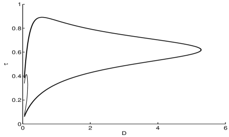
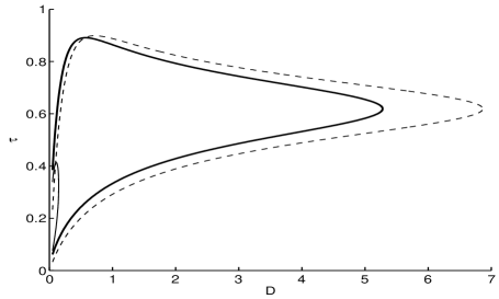
Figure 12: Hopf bifurcation boundaries in the $\tau$ versus $D$ plane for $m=2$, $r_{0}=0.25$, and with parameters as in (6.19), computed from (6.20). Left panel: the heavy solid curve and the solid curve are the Hopf bifurcation boundaries for the synchronous and asynchronous modes, respectively. Inside the respective lobes the corresponding mode is linearly unstable, as verified by the winding number criterion (6.22). Right panel: same plot except that we include the Hopf bifurcation boundary for the synchronous mode from the leading-order $D={D_{0}/\nu}\gg 1$ theory, computed from (3.17).

In Fig. 12 we plot the Hopf bifurcation boundaries when $m=2$ and $r_{0}=0.25$. From the left panel of this figure, the synchronous mode is unstable in the larger lobe shaped region, whereas the asynchronous mode is unstable only in the small lobe for small $D$, which is contained within the instability lobe for the synchronous mode. In the right panel of Fig. 12 we show the Hopf bifurcation boundary for the synchronous mode, as obtained from (3.17), corresponding to the leading-order $D={D_{0}/\nu}\gg 1$ theory. Since the instability lobe occurs for only moderate values of $D$, and $\epsilon=0.05$ is only moderately small, the leading-order theory from the $D={D_{0}/\nu}$ regime is, as expected, not particularly accurate in determining the Hopf bifurcation boundary. The fact that we have stability at a fixed $D$ for $\tau\gg 1$, which corresponds to very fast intracellular dynamics, is expected since in this limit the intracellular dynamics becomes decoupled from the bulk diffusion. Alternatively, if $\tau\ll 1$, then for a fixed $D$, the intracellular reactions proceed too slowly to create any instability. Moreover, in contrast to the large region of instability for the synchronous mode as seen in Fig. 12, we observe that the lobe of instability for the asynchronous mode only occurs for small values of $D$, where the diffusive coupling, and communication, between the two cells is rather weak. Somewhat more paradoxically, we also observe that the synchronous lobe of instability is bounded in $D$. This issue is discussed in more detail below.

In Fig. 13 we show the effect of changing the ring radius $r_{0}$ on the Hopf bifurcation boundaries. By varying $r_{0}$, we effectively are modulating the distance between the two cells. From this figure we observe that as $r_{0}$ is decreased, the lobe of instability for the asynchronous mode decreases, implying, rather intuitively, that at closer distances the two cells are better able to synchronize their oscillations than when they are farther apart. We remark that results from the leading-order theory of §3 for the $D={\mathcal{O}}(\nu^{-1})$ regime would be independent of $r_{0}$. We further observe from this figure that a synchronous instability can be triggered from a more clustered spatial arrangement of the cells inside the domain. In particular, for $D=5$ and $\tau=0.6$, we observe from Fig. 13 that we are outside the lobe of instability for $r_{0}=0.5$, but inside the lobe of instability for $r_{0}=0.25$ and $r_{0}=0.75$. We remark that due to the Neumann boundary conditions the cells on the ring with $r_{0}=0.75$ are close to two image cells outside the unit disk, which leads to a qualitatively similar clustering effect of these near-boundary cells as when they are on the small ring of radius $r_{0}=0.25$.

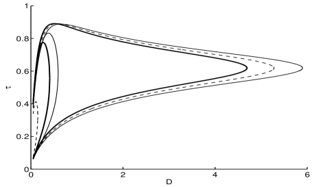
Figure 13: Hopf bifurcation boundaries for the synchronous mode (larger lobes) and the asynchronous mode (smaller lobes) in the $\tau$ versus $D$ plane for $m=2$ and for three values of $r_{0}$, with $r_{0}=0.5$ (heavy solid curves), $r_{0}=0.75$ (solid curves), and $r_{0}=0.25$ (dashed curves). The other parameters are given in (6.19). We observe that as $r_{0}$ decreases, where the two cells become more closely spaced, the lobe of instability for the asynchronous mode decreases.

In Fig. 14 we plot the Hopf bifurcation boundaries when $m=3$ and $r_{0}=0.5$. For $m=3$, we now observe that the region where the synchronous mode is unstable is unbounded in $D$. The lobe of instability for the asynchronous mode still exists only for small $D$, as shown in the right panel of Fig. 14. In this case, we observe that the Hopf bifurcation boundary for the synchronous mode, corresponding to the leading-order $D={D_{0}/\nu}\gg 1$ theory and computed from (3.17), now agrees rather well with results computed from (6.20).

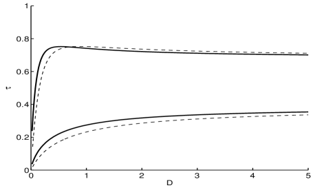
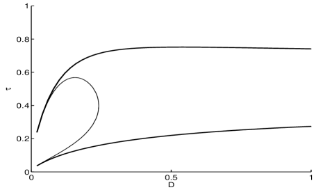
Figure 14: Left panel: Hopf bifurcation boundaries in the $\tau$ versus $D$ plane for the synchronous mode for $m=3$ equally-spaced cells on a ring of radius $r_{0}=0.50$ (heavy solid curves), as computed from (6.20), with parameters as in (6.19). The dashed curve is the Hopf bifurcation boundary from the leading-order $D={D_{0}/\nu}$ theory computed from (3.17). Right panel: The Hopf bifurcation boundaries for the asynchronous mode (solid curve) and the synchronous mode (heavy solid curve) shown in a magnified region of $D$. The asynchronous mode is linearly unstable only inside this small lobe, which lies within the unstable region for the synchronous mode.

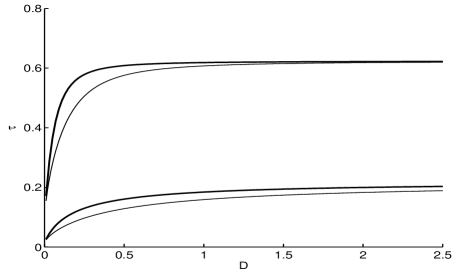
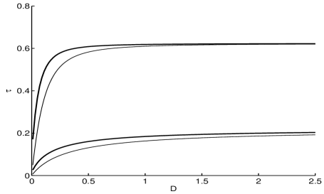
Figure 15: Left panel: Hopf bifurcation boundaries in the $\tau$ versus $D$ plane for the synchronous mode for $m=5$ equally-spaced cells on a ring of radius $r_{0}=0.25$ (solid curves) and radius $r_{0}=0.5$ (heavy solid curves) concentric with the unit disk, as computed from (6.20), with parameters (6.19). Right panel: Comparison of the Hopf bifurcation boundaries for the synchronous mode with $r_{0}=0.5$ (heavy solid curves), as computed from (6.20), with that obtained from (3.17) for the leading-order $D={D_{0}/\nu}$ theory (solid curves). These curves agree well when $D$ is large.

In the left panel of Fig. 15 we plot the Hopf bifurcation boundaries for the synchronous mode for $m=5$ when $r_{0}=0.5$ (heavy solid curves) and for $r_{0}=0.25$ (solid curves). We observe that for moderate values of $D$, the Hopf bifurcation values do depend significantly on the radius of the ring. The synchronous mode is unstable only in the infinite strip-like domain between these Hopf bifurcation boundaries. Therefore, only in some intermediate range of $\tau$, representing the ratio of the rates of the intracellular reaction and bulk decay, is the synchronous mode unstable. As expected, the two curves for different values of $r_{0}$ coalesce as $D$ increases, owing to the fact that the leading-order stability theory for $D={D_{0}/\nu}\gg 1$, as obtained from (3.17), is independent of $r_{0}$. In the right panel of Fig. 15 we compare the Hopf bifurcation boundaries for the synchronous mode with $r_{0}=0.5$ with that obtained from (3.17), corresponding to the leading-order theory in the $D={D_{0}/\nu\gg 1}$ regime. Rather curiously, we observe upon comparing the solid curves in the left and right panels in Fig. 15 that the Hopf bifurcation boundaries from the $D={\mathcal{O}}(1)$ theory when $r_{0}=0.25$, where the five cells are rather clustered near the origin, agree very closely with the leading order theory from the $D={D_{0}/\nu}\gg 1$ regime. Since the clustering of cells is effectively equivalent to a system with a large diffusion coefficient, this result above indicates, rather intuitively, that stability thresholds for a clustered spatial arrangement of cells will be more closely approximated by results obtained from a large $D$ approximation than for a non-clustered spatial arrangement of cells. In Fig. 16 we plot the Hopf bifurcation boundaries for the distinct asynchronous modes when $m=5$ for $r_{0}=0.5$ (left panel) and $r_{0}=0.75$ (right panel), as computed from (6.20) with $j=2,5$ (larger lobe) and with $j=3,4$ (smaller lobe). The asynchronous modes are only linearly unstable within these small lobes.

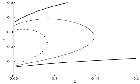
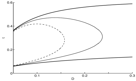
Figure 16: Hopf bifurcation boundaries for the two distinct asynchronous modes when $m=5$ for $r_{0}=0.5$ (left panel) and $r_{0}=0.75$ (right panel), as computed from (6.20) with $j=2,5$ (larger solid curve lobe) and with $j=3,4$ (smaller dashed curve lobe). The heavy solid curves are the Hopf bifurcation boundaries for the synchronous mode. The parameters are as in (6.19). The asynchronous mode for $j=2,5$ and $j=3,4$ is linearly unstable only inside the larger and smaller lobe, respectively.

To theoretically explain the observation that the instability region in the $\tau$ versus $D$ plane for the synchronous mode is bounded for $m=2$, but unbounded for $m\geq 3$, we must first extend the large $D$ analysis of §5 to the case of $m$ small cells. We readily derive, assuming identical behavior in each of the $m$ cells, that the reduced cell-bulk dynamics (5.16) for one cell must be replaced by

$$U_{0}^{\prime}=-\frac{1}{\tau}\left(1+\frac{2\pi md_{1}}{|\Omega|}\right)U_{0}+\frac{2\pi d_{2}m}{\tau|\Omega|}u_{1}\,,\qquad\boldsymbol{u}^{\prime}=\boldsymbol{F}(\boldsymbol{u})+\frac{2\pi}{\tau}\left[d_{1}U_{0}-d_{2}u_{1}\right]\boldsymbol{e}_{1}\,,$$ (6.23)

when there are $m$ cells. This indicates that the effective domain area is ${|\Omega|/m}={\pi/m}$ when there are $m$ cells. Therefore, to examine the stability of the steady-state solution of (6.23) for the Sel’kov model, we need only replace $|\Omega|$ with ${|\Omega|/m}$ in the Routh-Hurwitz criteria for the cubic (5.26).

With this approach, in Fig. 17 we show that there are two Hopf bifurcation values of $\tau$ for the steady-state solution of (6.23) when $m=3$ and $m=5$. These values correspond to the horizontal asymptotes as $D\to\infty$ in Fig. 14 for $m=3$ and in Fig. 15 for $m=5$. The numerical results from XPPAUT [5] in Fig. 17 then reveal the existence of a stable periodic solution branch connecting these Hopf bifurcation points for $m=3$ and $m=5$. A qualitatively similar picture holds for any $m\geq 3$. In contrast, for $m=2$, we can verify numerically using (5.26), where we replace $|\Omega|$ with ${|\Omega|/2}$, that the Routh-Hurwitz stability criteria $p_{1}>0$, $p_{3}>0$, and $p_{1}p_{2}>p_{3}$ hold for all $\tau>0$ when $m=2$ (and also $m=1$). Therefore, for $m=2$, there are no Hopf bifurcation points in $\tau$ for the steady-state solution of (6.23). This analysis suggests why there is a bounded lobe of instability for the synchronous mode when $m=2$, as was shown in Fig. 12.

We now suggest a qualitative reason for our observation that the lobe of instability for the synchronous mode is bounded in $D$ only when $m<m_{c}$, where $m_{c}$ is some threshold. We first observe that the diffusivity $D$ serves a dual role. Although larger values of $D$ allows for better communication between spatially segregated cells, suggesting that synchronization of their dynamics should be facilitated, it also has the competing effect of spatially homogenizing any perturbation in the diffusive signal. We suggest that only if the number of cells exceeds some threshold $m_{c}$, i.e. if some quorum is achieved, will the enhanced communication between the cells, resulting from a decrease in the effective domain area by ${|\Omega|/m}$, be sufficient to overcome the increased homogenizing effect of the diffusive signal at large values of $D$, and thereby lead to a synchronized time-periodic response.

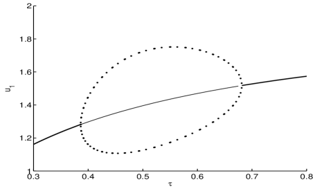
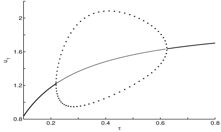
Figure 17: Global bifurcation diagram of $u_{1e}$ versus $\tau$ for the Sel’kov model (4.15) as computed using XPPAUT [5] from the ODE system (6.23) characterizing the limiting problem as $D\to\infty$ with $m$ small cells in the unit disk $\Omega$. Left panel: $m=3$. Right panel: $m=5$. The Sel’kov parameters are $\mu=2$, $\alpha=0.9$, and $\epsilon_{0}=0.15$, while $d_{1}=0.8$, and $d_{2}=0.2$. The thick/thin solid line represents stable/unstable steady-state solutions, while the solid dots indicate a stable synchronous periodic solution in the cells. For $m=5$ (right panel), there are two Hopf bifurcation points at $\tau=0.2187$ and $\tau=0.6238$. For $m=3$ (right panel), the two Hopf bifurcation points are at $\tau=0.3863$ and $\tau=0.6815$. These points correspond to the horizontal asymptotes as $D\to\infty$ in Fig. 15 for $m=5$ and in Fig. 14 for $m=3$.

7 Discussion and Outlook

We have formulated and studied a general class of coupled cell-bulk problems in 2-D with the primary goal of establishing whether such a class of problems can lead to the initiation of oscillatory instabilities due to the coupling between the cell and bulk. Our analysis relies on the assumption that the signaling compartments have a radius that is asymptotically small as compared to the length-scale of the domain. In this limit $\epsilon\to 0$ of small cell radius we have used a singular perturbation approach to determine the steady-state solution and to formulate the eigenvalue problem associated with linearizing around the steady-state. In the limit for which the bulk diffusivity $D$ is asymptotically large of order $D={\mathcal{O}}(\nu^{-1})$, we have derived eigenvalue problems characterizing the possibility of either synchronous and asynchronous instabilities triggered by the cell-bulk coupling. Phase diagrams in parameter space, showing where oscillatory instabilities can be triggered, were calculated for two specific choices of the intracellular kinetics. Our analysis shows that triggered oscillations are not possible when the intracellular dynamics has only one species. For the regime $D\gg{\mathcal{O}}(\nu^{-1})$, where the bulk can be effectively treated as a well-mixed system, and for the simple case of one cell, we have reduced the cell-bulk PDE system to a finite-dimensional ODE system for the spatially constant bulk concentration field coupled to the intracellular dynamics. This ODE system was shown to have triggered oscillations due to cell-bulk coupling, and global bifurcation diagrams were calculated for some specific reaction kinetics, showing that the branch of oscillatory solutions is globally stable. Finally, for the regime $D={\mathcal{O}}(1)$, where the spatial configuration of cells is an important factor, we have determined phase-diagrams for the initiation of synchronous temporal instabilities associated with a ring pattern of cells inside the unit disk, showing that such instabilities can be triggered from a more clustered spatial arrangement of the cells inside the domain.

We now discuss a few possible extensions of this study, and additional directions that warrant further investigation. For our choices of the intracellular kinetics used to illustrate the theory, the coupling between the bulk and cells leads to a unique steady-state solution. In contrast, it would be interesting to study more elaborate biologically relevant models, such as those in [21] and [17], where bistable and hysteric behavior of the steady-states is possible. In this way, the cell-bulk coupling and the spatial arrangement of the cells can possibly trigger transitions between different steady-state solutions. With regards to our basic model (2.1), it would be interesting to combine fast methods of potential theory (cf. [12]) to compute the eigenvalue-dependent Green’s function in (2.16) so as to obtain a hybrid analytical-numerical method to predict triggered cell-bulk oscillations from the GCEP (2.24). This would then allow us to readily consider random spatial configurations of $m$ cells in an arbitrary domain, rather than the simple ring patterns of cells studied in §6. In addition, it would be interesting to derive amplitude equations characterizing the weakly nonlinear development of any oscillatory linear instability for the coupled cell-bulk model. A weakly nonlinear analysis with an eigenvalue-dependent boundary condition was performed in [10] for the simpler, but related, problem of a coupled membrane-bulk model in 1-D. It would also be worthwhile to analyze large-scale oscillatory dynamics for the $D={\mathcal{O}}(1)$ regime in the limit $\epsilon\to 0$ in terms of the time-dependent Green’s function for the bulk diffusion process. From a numerical viewpoint, we further remark that for fixed $\epsilon$ a full numerical study of (2.1) does not appear to be possible with off-the-shelf PDE software owing to the rather atypical coupling between the bulk and the cells.

We now suggest two extensions of the model (2.1) that warrant further study. We first remark that for the well-mixed regime, where $D\gg{\mathcal{O}}(\nu^{-1})$, we can readily allow for a nonlinear bulk degradation, with possibly a Michaelis-Menton saturation, modeled by $\tau U_{t}=D\Delta U-\sigma_{B}(U)$, where $\sigma_{B}(U)={U/(1+cU)}$. With this modification, we can readily show, in place of (5.16), that the solution to the one cell-bulk model can be approximated by the finite-dimensional dynamics

$$U_{0}^{\prime}=-\frac{1}{\tau}\left(\sigma_{B}(U_{0})+\frac{2\pi d_{1}}{|\Omega|}U_{0}\right)+\frac{2\pi d_{2}}{\tau|\Omega|}u_{1}\,,\qquad\boldsymbol{u}^{\prime}=\boldsymbol{F}(\boldsymbol{u})+\frac{2\pi}{\tau}\left[d_{1}U_{0}-d_{2}u_{1}\right]\boldsymbol{e}_{1}\,.$$ (7.1)

It would be interesting to explore the effect of this nonlinear bulk decay on the possibility of Hopf bifurcations. Finally, as a second worthwhile direction, it would be interesting to study the stability of steady-state solutions to the coupled cell-bulk model when the intracellular dynamics $\boldsymbol{F}$ has a time-delay. Time-delays in reaction kinetics often occur in many biophysical systems, such as those involved with gene production (see [1], [2], [15], and the references therein). With such a delay, we expect that Hopf bifurcations can now occur with only one intracellular species in the regime $D={\mathcal{O}}(\nu^{-1})$.

Appendix A Non-Dimensionalization of the Coupled Cell-Bulk System

In this appendix we non-dimensionalize (1.1) into the dimensionless form (1.2). If we let $\left[\gamma\right]$ denote the dimensions of the variable $\gamma$, then the dimensions of the various quantities in (1.1) are as follows:

$$\left[{\mathcal{U}}\right] =\frac{\mbox{moles}}{\mbox{(length)}^{2}}\,,\qquad\left[\boldsymbol{\mu}\right]=\mbox{moles}\,,\qquad\left[\mu_{c}\right]=\mbox{moles}\,,\qquad\left[D_{B}\right]=\frac{\mbox{(length)}^{2}}{\mbox{time}}\,,\qquad$$ (A.1)

$$\left[k_{B}\right] =\left[k_{R}\right]=\frac{1}{\mbox{time}}\,,\qquad\left[\beta_{1}\right]=\frac{\mbox{length}}{\mbox{time}}\,,\qquad\ \left[\beta_{2}\right]=\frac{1}{\mbox{length}\times\mbox{time}}\,.$$

We now non-dimensionalize (1.1) by introducing the dimensionless variables $t$, $\boldsymbol{x}$, $U$, $\boldsymbol{u}$, and $D$, defined by

$$t=k_{R}T\,,\qquad\boldsymbol{x}={\boldsymbol{X}/L}\,,\qquad U=\frac{L^{2}}{\mu_{c}}{\mathcal{U}}\,,\qquad\boldsymbol{u}=\frac{\boldsymbol{\mu}}{\mu_{c}}\,,\qquad D\equiv\frac{D_{B}}{k_{B}L^{2}}\,,$$ (A.2)

where $L$ is a typical radius of $\Omega$. In terms of these variables, (1.1) becomes

$$\frac{k_{R}}{k_{B}}{U}_{t} =D\Delta_{\boldsymbol{x}}{U}-{U}\,,\qquad\boldsymbol{x}\in\tilde{\Omega}\backslash\tilde{\Omega}_{0}\,;\qquad\partial_{n_{\boldsymbol{x}}}{U}=0\,,\qquad\boldsymbol{x}\in\partial\tilde{\Omega}\,,$$ (A.3a)

$$D\partial_{n_{\boldsymbol{x}}}{U} =\frac{\beta_{1}}{k_{B}L}{U}-\frac{\beta_{2}L}{k_{B}}u^{1}\,,\;\;\quad\boldsymbol{x}\in\partial\tilde{\Omega}_{0}\,,$$

which is coupled to the intracellular dynamics

$$\frac{d\boldsymbol{u}}{dt}=\boldsymbol{F}\left(\boldsymbol{u}\right)+\frac{k_{B}\boldsymbol{e}_{1}}{k_{R}}\int_{\partial\tilde{\Omega}_{0}}\left(\frac{\beta_{1}}{k_{B}L}{U}-\frac{\beta_{2}L}{k_{B}}u^{1}\right)\,dS_{\boldsymbol{x}}\,.$$ (A.3b)

Here $\tilde{\Omega}_{0}$ is a disk centered at some $\boldsymbol{x}_{0}$ of radius ${\sigma/L}$. In our non-dimensionalization the time-scale is chosen based on the time-scale of the reaction kinetics, and $D$ is an effective dimensionless diffusivity $D$. In this way, and upon dropping the tilde variables, we obtain the dimensionless problem (1.2) with dimensionless parameters as in (1.3). We remark that upon using the divergence theorem, we can readily establish from (A.3) that

$$\frac{d}{dt}\left(\int_{\tilde{\Omega}\backslash{\tilde{\Omega}_{0}}}U\,d\boldsymbol{x}+\boldsymbol{e}^{T}\boldsymbol{u}\right)=-\frac{k_{B}}{k_{R}}\int_{\tilde{\Omega}\backslash{\tilde{\Omega}_{0}}}U\,d\boldsymbol{x}+\boldsymbol{e}^{T}\boldsymbol{F}(\boldsymbol{u})\,,$$ (A.4)

where $\boldsymbol{e}\equiv(1,\ldots,1)^{T}$. The left-hand side of this expression is the total amount of material inside the cells and in the bulk, while the right-hand side characterizes the bulk degradation and production within the cell.

References

- [1] S. N. Busenberg, J. M. Mahaffy, A compartmental reaction-diffusion cell cycle model, Computer Math. Applic. 18(10-11), (1989), pp. 883-892.
- [2] S. N. Busenberg, J. M. Mahaffy, The effects of dimension and size for a compartmental model of repression, SIAM J. Appl. Math., 48(4), (1988), pp. 882–903.
- [3] W. Chen, M. J. Ward, The stability and dynamics of localized spot patterns in the two-dimensional Gray-Scott model, SIAM J. Appl. Dyn. Sys., 10(2), (2011), pp. 582–666.
- [4] W. Y. Chiang, Y. X. Li, P. Y. Lai, Simple models for quorum sensing: Nonlinear dynamical analysis, Phys. Rev. E., 84, (2011), 041921.
- [5] G. B. Ermentrout, Simulating, analyzing, and animating dynamical systems: a guide to XPPAUT for researchers and students, SIAM 2002, Philadelphia, USA.
- [6] A. Goldbeter, Biochemical oscillations and cellular rhythms: The molecular bases of periodic and chaotic behaviour, Cambridge U. Press, Cambridge, U.K. (1990), 632 pp.
- [7] A. Gomez-Marin, J. Garcia-Ojalvo, J. M. Sancho, Self-sustained spatiotemporal oscillations induced by membrane-bulk coupling, Phys. Rev. Lett., 98(16), (2007), 168303.
- [8] J. Gou, Y. X. Li, W. Nagata, Interactions of in-phase and anti-phase synchronies in two cells coupled by a spatially diffusing chemical: double-hopf bifurcations, submitted, IMA J. Appl. Math., (July 2015), (23 pages).
- [9] J. Gou, M. J. Ward, Oscillatory dynamics for a coupled membrane-bulk diffusion model with Fitzhugh-Nagumo kinetics, under revision, SIAM J. Appl. Math., (2015), (23 pages).
- [10] J. Gou, Y. X. Li, W. Nagata, M. J. Ward Synchronized Oscillatory Dynamics for a 1-D Model of Membrane Kinetics Coupled by Linear Bulk Diffusion, to appear, SIAM J. Appl. Dyn. Sys., (2015), (37 pages).
- [11] L. Z. Krsmanovic, N. Mores, C. E. Navarro, K. K. Arora, K. J. Catt, An agonist-induced switch in g protein coupling of the gonadotropin-releasing hormone receptor regulates pulsatile neuropeptide secretion, Proc. Natl. Acad. Sci. USA, 100(5), (2003), pp. 2969–2974.
- [12] M. C. Kropinski, B. D. Quaife, Fast integral equation methods for the modified Helmholtz equation, J. Comp. Physics, 230(2), (2011), pp. 425–434.
- [13] V. Kurella, J. Tzou, D. Coombs, M. J. Ward, Asymptotic analysis of first passage time problems inspired by ecology, Bull. of Math Biology, 77(1), (2015), pp. 83–125.
- [14] C. Levy, D. Iron, Dynamics and stability of a three-dimensional model of cell signal transduction, J. Math. Bio., 67(6), (2014), pp. 1691–1728.
- [15] C. Levy, D. Iron, Dynamics and stability of a three-dimensional model of cell signal transduction with delay, Nonlinearity, 28(7), (2015), pp. 2515–2553.
- [16] Y. X. Li, A. Khadra, Robust Synchrony and Rhythmogenesis in Endocrine Neurons via Autocrine Regulations in Vitro and in Vivo, Bull. Math. Biology, 70(8), (2008), pp. 2103–2125.
- [17] J. Müller, C. Kuttler, B. A. Hense, M. Rothballer, A. Hartmann, Cell-cell communication by quorum sensing and dimension-reduction, J. Math. Biol., 53, (2006), pp. 672–702.
- [18] J. Müller, H. Uecker, Approximating the dynamics of communicating cells in a diffusive medium by ODEs - homogenization with localization, J. Math. Biol., 67, (2013), pp. 1023–1065.
- [19] F. Naqib, T. Quail, L. Musa, H. Vulpe, J. Nadeau, J. Lei, L. Glass, Tunable oscillations and chaotic dynamics in systems with localized synthesis, Phys. Rev. E., 85, (2012), 046210.
- [20] J. Noorbakhsh, D. Schwab, A. Sgro, T. Gregor, P. Mehta, Modeling oscillations and spiral waves in Dictyostelium populations, Phys. Rev. E. 91, 062711, (2015).
- [21] B. Novak, J. J. Tyson. Design principles of biochemical oscillators, Nat. Rev. Mol. Cell Biol., 9(12), (2008), pp. 981-991.
- [22] A. P. Peirce, H. Rabitz, Effect of defect structures on chemically active surfaces: a continuum approach, Phys. Rev. B., 38(3), (1998), pp. 1734–1753.
- [23] S. Pillay, M. J. Ward, A. Pierce, T. Kolokolnikov, An asymptotic analysis of the mean first passage time for narrow escape problems: Part I: Two-dimensional domains, SIAM Multiscale Model. Sim., 8(3), (2010), pp. 803–835.
- [24] H. Riecke, L. Kramer, Surface-induced chemical oscillations and their influence on space- and time- periodic patterns, J. Chem. Physics., 83, (1985), 3941.
- [25] I. Rozada, S. Ruuth, M. J. Ward, The stability of localized spot patterns for the Brusselator on the sphere, SIAM J. Appl. Dyn. Sys., 13(1), (2014), pp. 564–627.
- [26] M. J. Ward, Asymptotics for strong localized perturbations: Theory and applications, Online lecture notes for Fourth Winter School on Applied Mathematics, CityU of Hong Kong, (2010), (100 pages).
- [27] J. Wei, M. Winter, Spikes for the two-dimensional Gierer-Meinhardt system: the weak coupling case, J. Nonlinear Sci., 11(6), (2001), pp. 415–458.
- [28] J. Wei, M. Winter, Stationary multiple spots for reaction-diffusion systems, J. Math. Biol., 57(1), (2008), pp. 53–89.