From hard sphere dynamics to the Stokes-Fourier equations: an $L^{2}$ analysis of the Boltzmann-Grad limit

Abstract.

We derive the linear acoustic and Stokes-Fourier equations as the limiting dynamics of a system of $N$ hard spheres of diameter ${\varepsilon}$ in two space dimensions, when $N\to\infty$, ${\varepsilon}\to 0$, $N{\varepsilon}=\alpha\to\infty$, using the linearized Boltzmann equation as an intermediate step. Our proof is based on Lanford’s strategy [18], and on the pruning procedure developed in [5] to improve the convergence time to all kinetic times with a quantitative control which allows us to reach also hydrodynamic time scales. The main novelty here is that uniform $L^{2}$ a priori estimates combined with a subtle symmetry argument provide a weak version of chaos, in the form of a cumulant expansion describing the asymptotic decorrelation between the particles. A refined geometric analysis of recollisions is also required in order to discard the possibility of multiple recollisions.

1. Introduction to the Boltzmann-Grad limit and statement of the result

The sixth problem raised by Hilbert in 1900 on the occasion of the International Congress of Mathematicians addresses the question of the axiomatization of mechanics, and more precisely of describing the transition between atomistic and continuous models for gas dynamics by rigorous mathematical convergence results. Even though it is quite restrictive (since only perfect gases can be considered by this process), Hilbert further suggested using Boltzmann’s kinetic equation as an intermediate step to understand the appearance of irreversibility and dissipative mechanisms [15]. The derivation of the Boltzmann equation was then formalized in the pioneering work of Grad [12].

A huge amount of literature has been devoted to these asymptotic problems, but up to now they remain still largely open. Important breakthroughs [8, 3] have allowed for a complete study of some hydrodynamic limits of the Boltzmann equation, especially in incompressible viscous regimes leading to the Navier-Stokes equations (see [11] for instance). Note that other regimes such as the compressible Euler limit (which is the most immediate from a formal point of view) are still far from being understood [6, 20].

But, at this stage, the main obstacle seems actually to come from the other step, namely the derivation of the Boltzmann equation from a system of interacting particles: the best result to this day concerning this low density limit which is due to Lanford in the case of hard-spheres [18] (see also [7, 29, 9, 22, 23] for a complete proof) is indeed valid only for short times, i.e. breaks down before any relaxation can be observed.

Theorem 1.1.

Consider a system of $N$ hard-spheres of diameter ${\varepsilon}$ on $\mathbb{T}^{d}=[0,1]^{d}$ (with $d\geq 2$), initially “independent” and identically distributed with density $f_{0}$ such that

$$\big{\|}f_{0}\exp(\mu+\frac{\beta}{2}|v|^{2})\big{\|}_{L^{\infty}(\mathbb{T}^{d}_{x}\times\mathbb{R}^{d}_{v})}\leq 1\,,$$

for some $\beta>0,\mu\in\mathbb{R}$.

Fix $\alpha>0$, then, in the Boltzmann-Grad limit $N\to\infty$ with $N{\varepsilon}^{d-1}=\alpha$, the first marginal density converges almost everywhere to the solution of the Boltzmann equation

(1.1) $${\partial}_{t}f+v\cdot\nabla_{x}f=\alpha\,Q(f,f),$$

$$Q(f,f)(v):=\iint_{{\mathbb{S}}^{d-1}\times\mathbb{R}^{d}}[f(v^{\prime})f(v^{\prime}_{1})-f(v)f(v_{1})]\,\big{(}(v-v_{1})\cdot\nu\big{)}_{+}\,dv_{1}d\nu\,,$$

$$v^{\prime}=v+\nu\cdot(v_{1}-v)\,\nu\,,\quad v^{\prime}_{1}=v_{1}-\nu\cdot(v_{1}-v)\,\nu\,,$$

on a time interval $[0,C(\beta,\mu)/\alpha]$. As the propagation of chaos holds, the empirical measure converges in law to a density given by the solution of the Boltzmann equation.

By independent we mean here that the correlations, which are only due to the non overlapping condition, vanish asymptotically as ${\varepsilon}\to 0$.

The main reason why the convergence is not known to hold for longer time intervals is that the nonlinearity in the Boltzmann equation (1.1) is treated as if the equation was of the type $\partial_{t}f=\alpha f^{2}$: the cancellations between gain and loss terms in $Q(f,f)$ are yet to be understood. The only information we are able to get on these compensations comes from the stationarity of the canonical equilibrium measure. In this work, we consider very small fluctuations around such equilibria and show that the convergence is valid for all kinetic times with a quantitative control which allows us to reach also hydrodynamic time scales.

1.1. Setting of the problem

1.1.1. The model

In the following, we consider only the case of dimension $d=2$ (we refer the reader to Section 8.2 for a discussion of the difficulties to generalize our proof in higher dimensions). We are interested in describing the macroscopic behavior of a gas consisting of $N$ hard spheres of diameter ${\varepsilon}$ in a periodic domain ${\mathbb{T}^{2}}=[0,1]^{2}$ of $\mathbb{R}^{2}$, with positions and velocities $(x_{i},v_{i})_{1\leq i\leq N}$ in $({\mathbb{T}^{2}}\times\mathbb{R}^{2})^{N}$, the dynamics of which is given by

(1.2) $${dx_{i}\over dt}=v_{i}\,,\quad{dv_{i}\over dt}=0\quad\hbox{ as long as \ }|x_{i}(t)-x_{j}(t)|>{\varepsilon}\quad\hbox{for \ }1\leq i\neq j\leq N\,,$$

with specular reflection at a collision

(1.3) $$\left.\begin{aligned} v_{i}^{\prime}&:=v_{i}-\frac{1}{{\varepsilon}^{2}}(v_{i}-v_{j})\cdot(x_{i}-x_{j})\,(x_{i}-x_{j})\\ v_{j}^{\prime}&:=v_{j}+\frac{1}{{\varepsilon}^{2}}(v_{i}-v_{j})\cdot(x_{i}-x_{j})\,(x_{i}-x_{j})\end{aligned}\right\}\quad\hbox{ if }|x_{i}(t)-x_{j}(t)|={\varepsilon}\,.$$

By macroscopic behavior, we mean that we look for a statistical description both taking the limit $N\to\infty$ and averaging on the initial configurations.

Denote $X_{N}:=(x_{1},\dots,x_{N})\in\mathbb{T}^{2N}$, $V_{N}:=(v_{1},\dots,v_{N})\in\mathbb{R}^{2N}$ and $Z_{N}:=(X_{N},V_{N})\in\mathbb{D}^{N}$ where $\mathbb{D}^{N}:=\mathbb{T}^{2N}\times\mathbb{R}^{2N}$. Defining the Hamiltonian

$$H_{N}(V_{N}):=\frac{1}{2}\sum_{i=1}^{N}|v_{i}|^{2}\,,$$

we consider the Liouville equation in the $4N$-dimensional phase space

(1.4) $${\mathcal{D}}_{{\varepsilon}}^{N}:=\big{\{}Z_{N}\in\mathbb{D}^{N}\,/\,\forall i\neq j\,,\quad|x_{i}-x_{j}|>{\varepsilon}\big{\}}\,.$$

The Liouville equation is the following

$${\partial}_{t}f_{N}+\{H_{N},f_{N}\}=0\,,$$

or in other words

(1.5) $${\partial}_{t}f_{N}+V_{N}\cdot\nabla_{X_{N}}f_{N}=0\,,$$

with specular reflection on the boundary, meaning that if $Z_{N}$ belongs to ${\partial}{\mathcal{D}}_{{\varepsilon}}^{N+}(i,j)$ then we impose that

(1.6) $$f_{N}(t,Z_{N})=f_{N}(t,Z_{N}^{\prime})\,,$$

where $X_{N}^{\prime}=X_{N}$ and $v_{k}^{\prime}=v_{k}$ if $k\neq i,j$ while $(v_{i}^{\prime},v_{j}^{\prime})$ are given by (1.3). We have also defined

(1.7) $${\partial}{\mathcal{D}}_{{\varepsilon}}^{N\pm}(i,j):=\Big{\{}Z_{N}\in\mathbb{D}^{N}\,/\, |x_{i}-x_{j}|={\varepsilon}\,,\quad\pm(v_{i}-v_{j})\cdot(x_{i}-x_{j})>0$$

$$\mbox{and}\quad\forall(k,\ell)\in[1,N]^{2}\setminus\{(i,j)\}\,,k\neq\ell\,,|x_{k}-x_{\ell}|>{\varepsilon}\Big{\}}\,.$$

In the following we assume that $f_{N}$ is symmetric under permutations of the $N$ particles, meaning that the particles are exchangeable, and we define $f_{N}$ on the whole phase space $\mathbb{D}^{N}$ by setting $f_{N}\equiv 0$ on $\mathbb{D}^{N}\setminus{\mathcal{D}}_{{\varepsilon}}^{N}$.

We recall, as shown in [1] for instance, that the set of initial configurations leading to ill-defined characteristics (due to clustering of collision times, or collisions involving more than two particles) is of measure zero in ${\mathcal{D}}_{\varepsilon}^{N}$.

In the following we shall denote by ${\bf\Psi}_{N}$ the solution operator to the ODE (1.2-1.3) and by ${\bf S}_{N}$ the group associated with free transport in $\mathcal{D}_{\varepsilon}^{N}$ with specular reflection on the boundary. In other words, for a function $\varphi_{N}$ defined on $\mathcal{D}_{\varepsilon}^{N}$, we write

$${\bf S}_{N}(\tau)\varphi_{N}(Z_{N})=\varphi_{N}\big{(}{\bf\Psi}_{N}(-\tau)Z_{N}\big{)}\,.$$

1.1.2. The BBGKY and Boltzmann hierarchies

We are interested in the limiting behaviour of the previous system when $N\to\infty$ and ${\varepsilon}\to 0$ under the Boltzmann-Grad scaling $N{\varepsilon}=\alpha$, with $\alpha=O(1)$ or diverging slowly to infinity. The quantities which are expected to have finite limits in the Boltzmann-Grad limit are the marginals

$$f_{N}^{(s)}(t,Z_{s}):=\int_{\mathbb{D}^{N-s}}f_{N}(t,Z_{N})dz_{s+1}\dots dz_{N}$$

for every $s$ fixed ($s<N$).

A formal computation based on Green’s formula (see [7, 25, 9] for instance) leads to the following BBGKY hierarchy for $s<N$

(1.8) $$({\partial}_{t}+\sum_{i=1}^{s}v_{i}\cdot\nabla_{x_{i}})f_{N}^{(s)}(t,Z_{s})=\alpha\big{(}C_{s,s+1}f_{N}^{(s+1)}\big{)}(t,Z_{s})$$

on $\mathcal{D}_{\varepsilon}^{s}$, with the boundary condition as in (1.6)

$$f_{N}^{(s)}(t,Z_{s})=f_{N}^{(s)}(t,Z_{s}^{\prime})\hbox{ on }{\partial}D_{\varepsilon}^{s+}(i,j)\,.$$

The collision term is defined by

(1.9) $$\big{(}C_{s,s+1}f_{N}^{(s+1)}\big{)}(Z_{s}):=(N-s){\varepsilon}\alpha^{-1}$$

$$\times\Big{(}\sum_{i=1}^{s}\int_{{\mathbb{S}}\times\mathbb{R}^{2}}f_{N}^{(s+1)}(\dots,x_{i},v_{i}^{\prime},\dots,x_{i}+{\varepsilon}\nu,v^{\prime}_{s+1})\big{(}(v_{s+1}-v_{i})\cdot\nu\big{)}_{+}d\nu dv_{s+1}$$

$$\quad-\sum_{i=1}^{s}\int_{{\mathbb{S}}\times\mathbb{R}^{2}}f_{N}^{(s+1)}(\dots,x_{i},v_{i},\dots,x_{i}+{\varepsilon}\nu,v_{s+1})\big{(}(v_{s+1}-v_{i})\cdot\nu\big{)}_{-}d\nu dv_{s+1}\Big{)}$$

$$\mbox{with}\quad v_{i}^{\prime}:=v_{i}-(v_{i}-v_{s+1})\cdot\nu\,\nu\,,\quad v_{s+1}^{\prime}:=v_{s+1}+(v_{i}-v_{s+1})\cdot\nu\,\nu\,,$$

where ${\mathbb{S}}$ denotes the unit sphere in $\mathbb{R}^{2}$. Note that the collision integral is split into two terms according to the sign of $(v_{i}-v_{s+1})\cdot\nu$ and we used the trace condition on ${\partial}{\mathcal{D}}_{\varepsilon}^{N+}(i,s+1)$ to express all quantities in terms of pre-collisional configurations: in the following we shall also use the notation

$$C_{s,s+1}^{i,+}f_{s+1}(Z_{s}):=(N-s){\varepsilon}\alpha^{-1}\int f_{s+1}(\dots,x_{i},v_{i}^{\prime},\dots,x_{i}+{\varepsilon}\nu,v^{\prime}_{s+1})\Big{(}(v_{s+1}-v_{i})\cdot\nu\Big{)}_{+}d\nu dv_{s+1}\,,$$

$$C_{s,s+1}^{i,-}f_{s+1}(Z_{s}):=(N-s){\varepsilon}\alpha^{-1}\int f_{s+1}(\dots,x_{i},v_{i},\dots,x_{i}-{\varepsilon}\nu,v_{s+1})\Big{(}(v_{s+1}-v_{i})\cdot\nu\Big{)}_{+}d\nu dv_{s+1}\,,$$

so that

(1.10) $$C_{s,s+1}=\sum_{i=1}^{s}(C_{s,s+1}^{i,+}-C_{s,s+1}^{i,-})\,.$$

The closure for $s=N$ is given by the Liouville equation (1.5).

To obtain the Boltzmann hierarchy, we compute the formal limit of the transport and collision operators when ${\varepsilon}$ goes to $0$. Recalling that $(N-s){\varepsilon}\sim\alpha$, the limit hierarchy is given by

(1.11) $$({\partial}_{t}+\sum_{i=1}^{s}v_{i}\cdot\nabla_{x_{i}})f^{(s)}(t,Z_{s})=\alpha\big{(}\bar{C}_{s,s+1}f^{(s+1)}\big{)}(t,Z_{s})\,,$$

in $\mathbb{D}^{s}$, where $\bar{C}_{s,s+1}$ are the limit collision operators defined by

$$\big{(}\bar{C}_{s,s+1}f^{(s+1)}\big{)}(Z_{s}) :=\sum_{i=1}^{s}\int f^{(s+1)}(\dots,x_{i},v_{i}^{\prime},\dots,x_{i},v^{\prime}_{s+1})\Big{(}(v_{s+1}-v_{i})\cdot\nu\Big{)}_{+}d\nu dv_{s+1}$$

$$\quad-\sum_{i=1}^{s}\int f^{(s+1)}(\dots,x_{i},v_{i},\dots,x_{i},v_{s+1})\Big{(}(v_{s+1}-v_{i})\cdot\nu\Big{)}_{+}d\nu dv_{s+1}\,.$$

1.1.3. Initial data and closures for the Boltzmann hierarchy

Consider chaotic initial data of the form $(f_{0}^{\otimes s})_{s\in\mathbb{N}^{*}}$, with

$$f_{0}^{\otimes s}(Z_{s}):=\prod_{i=1}^{s}f_{0}(z_{i})\quad\text{with}\quad\int_{\mathbb{D}}f_{0}(z)dz=1\,,$$

and denote by $f(t)$ the solution of the nonlinear Boltzmann equation (1.1) which can be rewritten as

$$({\partial}_{t}+v\cdot\nabla_{x})f=\alpha\bar{C}_{1,2}f^{\otimes 2}\,,\qquad f_{|t=0}=f_{0}\,.$$

Then an easy computation shows that $(f(t)^{\otimes s})_{s\in\mathbb{N}^{*}}$ is a chaotic solution to the Boltzmann hierarchy, whose first marginal is nothing else than $f(t)$. Note that, even though it may look like a very particular case, it is somehow generic as any symmetric initial datum may in fact be decomposed as a superposition of chaotic distributions (this is known as the Hewitt-Savage theorem, see [14]). This means that the Boltzmann hierarchy, even though consisting of linear equations, encodes nonlinear phenomena. In the absence of suitable uniform a priori estimates, we therefore may expect the solution to blow up after a finite time. This is actually the main obstacle to get a rigorous derivation of the Boltzmann equation over time intervals larger than the mean free time $O(1/\alpha)$.

A different structure of initial datum can lead to other types of equations. Recall that the Maxwellian

$$M_{\beta}(v):={\beta\over 2\pi}\exp\left(-\beta{|v|^{2}\over 2}\right)$$

is an equilibrium for the Boltzmann dynamics, so that $(M_{\beta}^{\otimes s})_{s\geq 1}$ is a stationary solution to the Boltzmann hierarchy. Consider an initial datum which is a perturbation of this stationary solution

(1.12) $$f^{(s)}_{0}(Z_{s})=M_{\beta}^{\otimes s}(V_{s})\sum_{i=1}^{s}g_{\alpha,0}(z_{i})\,,$$

where we added a dependency of $g_{\alpha,0}$ on $\alpha$ for later purposes. This form is stable under the limit dynamics [4] so that a solution to the Boltzmann hierarchy (1.11) is

(1.13) $$f^{(s)}(t,Z_{s})=M_{\beta}^{\otimes s}(V_{s})\sum_{i=1}^{s}g_{\alpha}(t,z_{i})$$

where $g_{\alpha}$ is a solution of the linearized Boltzmann equation

(1.14) $$({\partial}_{t}+v\cdot\nabla_{x})g_{\alpha}=-\alpha\mathcal{L}_{\beta}g_{\alpha}\,,$$

$$\mathcal{L}_{\beta}\,g_{\alpha}(v):=-{1\over M_{\beta}}\bar{C}_{1,2}(M_{\beta}\otimes M_{\beta}g_{\alpha}+M_{\beta}g_{\alpha}\otimes M_{\beta})(v)$$

$$\qquad\qquad=\int M_{\beta}(v_{1})\Big{(}g_{\alpha}(v)+g_{\alpha}(v_{1})-g_{\alpha}(v^{\prime})-g_{\alpha}(v_{1}^{\prime})\Big{)}\Big{(}(v_{1}-v)\cdot\nu\Big{)}_{+}d\nu dv_{1}\,,$$

with initial datum $g_{\alpha,0}$. The functional space $L^{2}(dxM_{\beta}dv)$ is natural to study the linearized Boltzmann equation, because the associate norm is a Lyapunov functional for (1.14) (see Appendix A). As we will heavily use it later on, we introduce the following notation, for $p=1,2$: for any function $g_{s}$ defined on $\mathbb{D}^{s}$,

(1.15) $$\|g_{s}\|_{L^{p}_{\beta}(\mathbb{D}^{s})}:=\Big{(}\int M^{\otimes s}_{\beta}(V_{s})|g_{s}|^{p}(Z_{s})\,dZ_{s}\Big{)}^{\frac{1}{p}}\,.$$

We now turn to the particle dynamics and discuss the counterpart of the initial datum (1.12). The Gibbs measure

(1.16) $$M_{N,\beta}(Z_{N}):=\frac{1}{\mathcal{Z}_{N}}{\bf 1}_{\mathcal{D}_{\varepsilon}^{N}}(X_{N})\,M_{\beta}^{\otimes N}(V_{N})\,,\qquad\mathcal{Z}_{N}:=\int_{\mathbb{T}^{2N}}\prod_{1\leq i\neq j\leq N}{\bf 1}_{|x_{i}-x_{j}|>{\varepsilon}}\,dX_{N}$$

is invariant for the dynamics. An idea to get such linear asymptotics as (1.13) is to consider small fluctuations around an equilibrium of the form

$$f_{N,0}(Z_{N})=M_{N,\beta}(Z_{N})\prod_{i=1}^{N}\big{(}1+\delta g_{\alpha,0}(z_{i})\big{)}\,.$$

However whatever the smallness of $\delta$, such a sequence of initial data is never a small correction to $M_{N,\beta}$. Thus, we shall tune the size of the perturbation with $N$

$$f_{N,0}(Z_{N}) =M_{N,\beta}(Z_{N})\prod_{i=1}^{N}\big{(}1+\frac{\delta}{N}g_{\alpha,0}(z_{i})\big{)}$$

(1.17) $$=M_{N,\beta}(Z_{N})+\frac{\delta}{N}M_{N,\beta}(Z_{N})\sum_{i=1}^{N}g_{\alpha,0}(z_{i})+O(\delta^{2})\,.$$

At the first order in ${\delta}{}$, we recover an initial datum for the BBGKY hierarchy of the form (1.12)

(1.18) $$f_{N,0}(Z_{N})=M_{N,\beta}(Z_{N})\sum_{i=1}^{N}g_{\alpha,0}(z_{i})\quad\hbox{ with }\quad\int M_{\beta}g_{\alpha,0}(z)dz=0\,.$$

This initial datum records only the perturbation and it is no longer a probability measure. In particular

$$\int f_{N,0}(Z_{N})dZ_{N}=0\,,$$

and this property is preserved by the Liouville equation (1.5). The question is then to know if the solution of the BBGKY hierarchy obeys a form similar to (1.13), at least approximately, and if one can obtain good enough bounds in $L^{2}$ spaces to prove long-time convergence of the marginals to $f^{(s)}$ defined in (1.13).

Remark 1.1.

Note that another type of (non symmetric) perturbation was dealt with in [5], namely an initial datum of the form

(1.19) $$f_{N,0}(Z_{N})=M_{N,\beta}(Z_{N})g_{0}(z_{1})\,.$$

This describes the motion of a tagged particle in a background close to equilibrium, and we have shown that it satisfies asymptotically the linear Boltzmann equation, and the tagged particle dynamics converges to the Brownian motion in the diffusive limit. However the proof is less complicated since all quantities of interest are uniformly controlled in $L^{\infty}$, which will not be the case with the initial datum (1.18).

1.2. Statement of the results

1.2.1. Low density limit

Our main result is the following.

Theorem 1.2.

Consider $N$ hard spheres on the space $\mathbb{D}=\mathbb{T}^{2}\times\mathbb{R}^{2}$, initially distributed according to $f_{N,0}$ defined as in (1.18) where $g_{\alpha,0}$ is a bounded, Lipschitz function on $\mathbb{D}$ with zero average, and satisfying the following bound for some constant $C_{1}$

(1.20) $$\|g_{\alpha,0}\|_{W^{1,\infty}}\leq C_{1}\exp(C_{1}\alpha^{2})\,.$$

Then the one-particle distribution $f_{N}^{(1)}(t,z)$ is close to $M_{\beta}(v)g_{\alpha}(t,z)$, where $g_{\alpha}(t,z)$ is the solution of the linearized Boltzmann equation (1.14) with initial datum $g_{\alpha,0}(z)$.

More precisely, there exists a non negative constant $C$ such that for all $T>1$ and all $\alpha>1$, in the limit $N\to\infty$, $N\varepsilon\alpha^{-1}=1$,

(1.21) $$\sup_{t\in[0,T]}\big{\|}f_{N}^{(1)}(t)-M_{\beta}g_{\alpha}(t)\big{\|}_{L^{2}(\mathbb{D})}\leq\frac{T^{2}e^{C\alpha^{2}}}{\sqrt{\log\log N}}\,\cdotp$$

Note that the $L^{\infty}$-convergence to the solution of the linearized equation was established in [4] following Lanford’s strategy. This convergence was derived for short times, but in any dimension $d\geq 3$. The generalization out of equilibrium was then established in [28].

Following [4], Theorem 1.2 can also be interpreted as the limit of time correlations in the fluctuation field at equilibrium. Let $h$ be a smooth function in $\mathbb{T}^{2}\times\mathbb{R}^{2}$ such that $\int M_{\beta}h(z)dz=0$, then the fluctuation field $\zeta^{N}$ can be tested against $h$ at time $t$

$$\zeta^{N}(h,Z_{N}(t)):=\frac{1}{\sqrt{N}}\sum_{i=1}^{N}h(z_{i}(t))\,,$$

where $Z_{N}(t)$ stands for the particle configuration at time $t$. The equilibrium covariance of the fluctuation field at different times, say 0 and $t$, is given by

$${\mathbb{E}}_{M_{N,\beta}}\left(\zeta^{N}(h,Z_{N}(0))\zeta^{N}(\tilde{h},Z_{N}(t))\right)=\int_{\mathbb{T}^{2N}\times\mathbb{R}^{2N}}M_{N,\beta}(Z_{N})\,\zeta^{N}(h,Z_{N}(0))\zeta^{N}(\tilde{h},Z_{N}(t))\,,$$

for all smooth functions $h,\tilde{h}$ in $\mathbb{T}^{2}\times\mathbb{R}^{2}$ with mean 0. Using an initial datum of the form (1.18)

$$f_{N,0}(Z_{N})=M_{N,\beta}(Z_{N})\sum_{i=1}^{N}h(z_{i})\quad\hbox{ with }\quad\int M_{\beta}h(z)dz=0\,,$$

the covariance can be rewritten, thanks to the exchangeability of the particles, as

$${\mathbb{E}}_{M_{N,\beta}}\left(\zeta^{N}(h,Z_{N}(0))\zeta^{N}(\tilde{h},Z_{N}(t))\right) =\int_{\mathbb{T}^{2N}\times\mathbb{R}^{2N}}dZ_{N}\,f_{N,0}(Z_{N})\,\frac{\sum_{i=1}^{N}\tilde{h}(z_{i}(t))}{N}$$

$$=\int_{\mathbb{D}}dz_{1}f_{N}^{(1)}(t,z_{1})\tilde{h}(z_{1})\,.$$

Thus the limiting time covariance is related to the convergence of the first marginal $f_{N}^{(1)}$ and the following corollary is an immediate consequence of Theorem 1.2.

Corollary 1.2.

Fix $\alpha>0$ and let $h,\tilde{h}$ be two functions in $L^{2}_{\beta}(\mathbb{D})$ with mean 0 with respect to $M_{\beta}dvdx$. Then for any $t\geq 0$, the time covariance converges in the Boltzmann-Grad limit $N\to\infty$, $N\varepsilon\alpha^{-1}=1$

$$\lim_{N\to\infty} {\mathbb{E}}_{M_{N,\beta}}\left(\zeta^{N}(h,Z_{N}(0))\zeta^{N}(\tilde{h},Z_{N}(t))\right)$$

$$=\int_{\mathbb{T}^{2}\times\mathbb{R}^{2}}dz\,M_{\beta}(v)\exp\big{(}-t(v\cdot\nabla_{x}+\alpha\mathcal{L}_{\beta})\big{)}h(z)\;\tilde{h}(z),$$

where $v\cdot\nabla_{x}+\alpha\mathcal{L}_{\beta}$ is the operator associated with the linearized Boltzmann equation (1.14).

Correlation functions are cornerstones of statistical mechanics and besides the case of mean field models, mathematical results on these correlations are sparse in the context of classical interacting $n$-body systems (see nevertheless [19] for an explicit computation in the case of one dimensional hard rods). The convergence of the fluctuation field (for arbitrary time) to a stationary Ornstein-Uhlenbeck process was derived in [24] for a related microscopic dynamics with random collisions. A similar convergence of the fluctuation field for the Hamiltonian dynamics is conjectured in [27], but its derivation would require a better understanding of the emergence of the noise arising from the deterministic evolution.

1.2.2. Hydrodynamic limits

Once Theorem 1.2 is known, it is possible to take the limit $\alpha\to\infty$ while conserving a small error on the right-hand side of (1.21). Using the classical convergence of the linearized Boltzmann equation to the acoustic equation (see Appendix A), one infers the following result.

Corollary 1.3.

Consider $N$ hard spheres on the space $\mathbb{D}=\mathbb{T}^{2}\times\mathbb{R}^{2}$, initially distributed according to $f_{N,0}$ defined as in (1.18) with a sequence $(g_{\alpha,0})$ of functions satisfying the assumptions of Theorem 1.2 and converging in $L^{2}_{\beta}(\mathbb{D})$ as $\alpha$ diverges to

$$g_{0}(x,v):=\rho_{0}(x)+\sqrt{\beta}\,u_{0}(x)\cdot v+\frac{\beta|v|^{2}-2}{2}\,\theta_{0}(x)\quad\text{with}\quad\int_{\mathbb{T}^{2}}\rho_{0}(x)dx=0\,.$$

Then as $N\to\infty$, $N\varepsilon=\alpha\to\infty$ much slower than $\sqrt{\log\log\log N}$, the distribution $f_{N}^{(1)}(t)$ converges in $L^{2}(\mathbb{D})$-norm to $M_{\beta}g(t)$ with

$$g(t,x,v):=\rho(t,x)+\sqrt{\beta}\,u(t,x)\cdot v+\frac{\beta|v|^{2}-2}{2}\theta(t,x)\,,$$

where $(\rho,u,\theta)$ satisfies the acoustic equations

$$\left\{\begin{aligned} &{\partial}_{t}\rho+\frac{1}{\sqrt{\beta}}\,\nabla_{x}\cdot u=0\\ &{\partial}_{t}u+\frac{1}{\sqrt{\beta}}\,\nabla_{x}(\rho+\theta)=0\\ &{\partial}_{t}\theta+\frac{1}{\sqrt{\beta}}\,\nabla_{x}\cdot u=0\\ \end{aligned}\right.$$

with initial datum $(\rho_{0},u_{0},\theta_{0})$.

It is even possible to rescale time as $t=\alpha\tau$ and to take the limit $\alpha\to\infty$. For well-prepared initial data, we then obtain the following diffusive approximation by the Stokes-Fourier dynamics.

Corollary 1.4.

Consider $N$ hard spheres on the space $\mathbb{D}=\mathbb{T}^{2}\times\mathbb{R}^{2}$, initially distributed according to $f_{N,0}$ defined in (1.18) with a sequence $(g_{\alpha,0})$ of functions satisfying the assumptions of Theorem 1.2 and converging in $L^{2}_{\beta}$ as $\alpha\to\infty$ to

$$g_{0}(x,v):=\sqrt{\beta}\,u_{0}(x)\cdot v+\frac{\beta|v|^{2}-4}{2}\,\theta_{0}(x)\,,\quad\nabla_{x}\cdot u_{0}=0\,.$$

Then as $N\to\infty$, $N\varepsilon=\alpha\to\infty$ much slower than $\sqrt{\log\log\log N}$, the distribution $f_{N}^{(1)}(\alpha\tau)$ converges in $L^{2}(\mathbb{D})$ norm to $M_{\beta}g(\tau)$ with

$$g(\tau,x,v):=\sqrt{\beta}\,u(\tau,x)\cdot v+\frac{\beta|v|^{2}-4}{2}\theta(\tau,x)\,,$$

where $(u,\theta)$ satisfies the Stokes-Fourier equations

(1.22) $$\left\{\begin{aligned} &\partial_{\tau}u-\frac{1}{\sqrt{\beta}}\,\mu_{\beta}\Delta_{x}u=0\\ &\nabla_{x}\cdot u=0\\ &\partial_{\tau}\theta-\frac{1}{\sqrt{\beta}}\,\kappa_{\beta}\Delta_{x}\theta=0\\ \end{aligned}\right.$$

with initial datum $(u_{0},\theta_{0})$, and

$$\mu_{\beta}:=\frac{1}{4}\int\Phi_{\beta}\mathcal{L}_{\beta}^{-1}\Phi_{\beta}M_{\beta}(v)dv\quad\hbox{ with }\quad\Phi_{\beta}(v):=\beta^{2}(v\otimes v-{|v|^{2}\over 2}{\rm{Id}})\,,$$

$$\kappa_{\beta}:=\frac{1}{4}\int\Psi_{\beta}\mathcal{L}_{\beta}^{-1}\Psi_{\beta}M_{\beta}(v)dv\quad\hbox{ with }\quad\Psi_{\beta}(v):=\sqrt{\beta}\,v\left(\beta{|v|^{2}\over 4}-1\right)\,,$$

where the operator $\mathcal{L}_{\beta}$ was introduced in (1.14).

Remark 1.5.

In the case of general, ill-prepared initial data, the asymptotics is also well known [10]. Details are provided in Appendix A.

Acknowledgements. We would like to thank Herbert Spohn and Sergio Simonella for their careful reading of our paper and very useful suggestions.

2. Strategy of the proof

In what follows, we focus on the proof of Theorem 1.2, as it is the new contribution of this work. Even though it follows some ideas introduced in [5], it represents a real improvement of what has been done up to now:

• First of all, we are able to capture a fluctuation of order $O(1/N)$ around an equilibrium (1.17), and in particular there is no more positivity.

• Second, we deal with a much weaker functional setting than the $L^{\infty}$ framework of Lanford’s strategy [18], which leads to major difficulties to give sense to the collision operator (defined as an integral over a singular set).

• The strategy developed here to bypass this obstacle uses crucially the exchangeability to get a weak version of chaos independently of the precise structure of the initial datum. This seems to be an important conceptual progress.

Let us recall that, up to now, all the results regarding the low density limit of deterministic systems of particles have been established following Lanford’s strategy [18]. In this section, we describe the main objects involved in the proof, and the pruning procedure introduced in [5]. We then show the main differences between our setting and that of [5] and finally explain how to adapt the pruning procedure to our setting.

2.1. The series expansion

The starting point is the series expansion obtained by iterating Duhamel’s formula for the BBGKY hierarchy (1.8)

(2.1) $$f^{(s)}_{N}(t)=\sum_{n=0}^{N-s}\alpha^{n}\int_{0}^{t}\int_{0}^{t_{s+1}}\dots\int_{0}^{t_{s+n-1}}{\bf S}_{s}(t-t_{s+1})C_{s,s+1}{\bf S}_{s+1}(t_{s+1}-t_{s+2})C_{s+1,s+2}$$

$$\dots\bf S_{s+n}(t_{s+n})f^{(s+n)}_{N,0}\>dt_{s+n}\dots dt_{s+1}\,,$$

where ${\bf S}_{s}$ denotes the group associated with free transport in $\mathcal{D}_{\varepsilon}^{s}$ with specular reflection on the boundary. By abuse of notation, the term $n=0$ in (2.1) should be interpreted as ${\bf S}_{s}(t)f^{(s)}_{N,0}$ as $n$ records the number of collision operators up to time 0. Denoting by ${\bf S}_{s}^{0}$ the free flow, one can derive formally the limiting Boltzmann hierarchy

(2.2) $$f^{(s)}(t)=\sum_{n\geq 0}\alpha^{n}\int_{0}^{t}\int_{0}^{t_{s+1}}\dots\int_{0}^{t_{s+n-1}}{\bf S}^{0}_{s}(t-t_{s+1})\bar{C}_{s,s+1}{\bf S}^{0}_{s+1}(t_{s+1}-t_{s+2})\bar{C}_{s+1,s+2}$$

$$\dots\bf S^{0}_{s+n}(t_{s+n})f^{(s+n)}_{0}\>dt_{s+n}\dots dt_{s+1}\,,$$

and one aims at proving the convergence of one hierarchy to the other.

These series expansions have graphical representations which play a key role in the analysis as explained first in [18, 7, 25, 9, 22, 23]. This interpretation in terms of collision trees is described below.

Let us extract combinatorial information from the iterated Duhamel formula (2.1). We describe the adjunction of new particles (in the backward dynamics) by ordered trees.

Definition 2.1 (Collision trees).

Let $s>1$ be fixed. An (ordered) collision tree $a\in\mathcal{A}_{s}$ is defined by a family $(a(i))_{2\leq i\leq s}$ with $a(i)\in\{1,\dots,i-1\}$.

Note that  $|\mathcal{A}_{s}|\leq(s-1)!$.

Once we have fixed a collision tree $a\in\mathcal{A}_{s}$, we can reconstruct pseudo-dynamics starting from any point in the one-particle phase space $z_{1}=(x_{1},v_{1})\in\mathbb{T}^{2}\times\mathbb{R}^{2}$ at time $t$.

Definition 2.2 (Pseudo-trajectory).

Given $z_{1}\in\mathbb{T}^{2}\times\mathbb{R}^{2}$, $t>0$ and a collision tree $a\in\mathcal{A}_{s}$, consider a collection of times, angles and velocities $(T_{2,s},\Omega_{2,s},V_{2,s})=(t_{i},\nu_{i},v_{i})_{2\leq i\leq s}$ with $0\leq t_{s}\leq\dots\leq t_{2}\leq t$. We then define recursively the pseudo-trajectories in terms of the backward BBGKY dynamics as follows

• in between the collision times $t_{i}$ and $t_{i+1}$ the particles follow the $i$-particle backward flow with specular reflection;

• at time $t_{i}^{+}$, particle $i$ is adjoined to particle $a(i)$ at position $x_{a(i)}(t_{i}^{+})+{\varepsilon}\nu_{i}$ and with velocity $v_{i}$, provided $|x_{i}-x_{j}(t_{i}^{+})|>{\varepsilon}$ for all $j<i$ with $j\neq a(i)$. If $(v_{i}-v_{a(i)}(t_{i}^{+}))\cdot\nu_{i}>0$, velocities at time $t_{i}^{-}$ are given by the scattering laws

  (2.3) $$v_{a(i)}(t^{-}_{i}) =v_{a(i)}(t_{i}^{+})-(v_{a(i)}(t_{i}^{+})-v_{i})\cdot\nu_{i}\,\nu_{i}\,,$$

  $$v_{i}(t^{-}_{i}) =v_{i}+(v_{a(i)}(t_{i}^{+})-v_{i})\cdot\nu_{i}\,\nu_{i}\,.$$

We denote by $z_{i}(a,T_{2,s},\Omega_{2,s},V_{2,s},\tau)$ the position and velocity of the particle labeled $i$, at time $\tau$ (provided $\tau<t_{i}$). The configuration obtained at the end of the tree, i.e. at time 0, is $Z_{s}(a,T_{2,s},\Omega_{2,s},V_{2,s},0)$.

Similarly, we define the pseudo-trajectories associated with the Boltzmann hierarchy. These pseudo-trajectories evolve according to the backward Boltzmann dynamics as follows

• in between the collision times $t_{i}$ and $t_{i+1}$ the particles follow the $i$-particle backward free flow;

• at time $t_{i}^{+}$, particle $i$ is adjoined to particle $a(i)$ at exactly the same position $x_{a(i)}(t_{i}^{+})$. Velocities are given by the laws (2.3).

We denote $\bar{Z}_{s}(a,T_{2,s},\Omega_{2,s},V_{2,s},0)$ the initial configuration.

The definition of a pseudo-trajectory in the BBGKY dynamics is subject to the fact that particles cannot overlap. This is recorded in the next definition.

Definition 2.3 (Non overlapping sets).

Given $z_{1}\in\mathbb{T}^{2}\times\mathbb{R}^{2}$ and a collision tree $a\in\mathcal{A}_{s}$, the non-overlapping set is defined by

$$G_{s}(a):=\Big{\{}(T_{2,s},\Omega_{2,s},V_{2,s}) \in\mathcal{T}_{2,s}\times{\mathbb{S}}^{s-1}\times\mathbb{R}^{2(s-1)}\,\Big{|}$$

$$\text{there exists \ }Z_{s}(a,T_{2,s},\Omega_{2,s},V_{2,s},0)\,\text{ a pseudo-trajectory}\Big{\}}\,,$$

denoting

$$\mathcal{T}_{2,s}:=\big{\{}(t_{i})_{2\leq i\leq s}\in[0,t]^{s-1}\,/\,0\leq t_{s}\leq\dots\leq t_{2}\leq t\big{\}}\,.$$

The following semantic distinction will be important later on.

Definition 2.4 (Collisions/Recollisions).

In the BBGKY hierarchy, the term collision will be used only for the creation of a new particle, i.e. for a branching in the collision trees. A shock between two particles in the backward BBGKY dynamics will be called a recollision.

Note that no recollision occurs in the Boltzmann hierarchy as the particles have zero diameter.

With these notations, the iterated Duhamel formula (2.1) for the first marginal ($s=1$) can be rewritten

(2.4) $$f^{(1)}_{N}(t)=\sum_{s=1}^{N}(N-1)\dots\big{(}N-(s-1)\big{)}{\varepsilon}^{s-1}\sum_{a\in\mathcal{A}_{s}}\int_{G_{s}(a)} dT_{2,s}d\Omega_{2,s}dV_{2,s}\Big{(}\prod_{i=2}^{s}\big{(}(v_{i}-v_{a(i)}(t_{i}))\cdot\nu_{i}\Big{)}$$

$$\quad\times f_{N,0}^{(s)}\big{(}Z_{s}(a,T_{2,s},\Omega_{2,s},V_{2,s},0)\big{)}\,,$$

while in the limit

(2.5) $$f^{(1)}(t)=\sum_{s=1}^{\infty}\alpha^{s-1}\sum_{a\in\mathcal{A}_{s}}\int_{\mathcal{T}_{2,s}\times{\mathbb{S}}^{s-1}\times\mathbb{R}^{2(s-1)}} dT_{2,s}d\Omega_{2,s}dV_{2,s}\Big{(}\prod_{i=2}^{s}(v_{i}-v_{a(i)}(t_{i}))\cdot\nu_{i}\Big{)}$$

$$\quad\times f_{0}^{(s)}\big{(}\bar{Z}_{s}(a,T_{2,s},\Omega_{2,s},V_{2,s},0)\big{)}\,.$$

2.2. Lanford’s strategy

Lanford’s proof relies then on two steps :

• proving a short time bound for the series (2.4) expressing the correlations of the system of $N$ particles and a similar bound for the corresponding quantities associated with the Boltzmann hierarchy;

• proving the convergence of each term of the series, i.e. proving that the BBGKY and Boltzmann pseudo-trajectories $Z_{s}(a,T_{2,s},\Omega_{2,s},V_{2,s},0)$ and $\bar{Z}_{s}(a,T_{2,s},\Omega_{2,s},V_{2,s},0)$ stay close to each other, outside a set of parameters $(t_{i},\nu_{i},v_{i})_{2\leq i\leq s}$ of vanishing measure.

Note that step (i) alone is responsible for the fact that the low density limit is only known to hold for short times (of the order of $1/\alpha$). This is due to the fact that the uniform bound is essentially obtained by replacing the hierarchy by the one related to an equation of the type $\partial_{t}f=\alpha f^{2}$, neglecting all cancellations present in the collision term.

More precisely, defining the operator associated with the series (2.1)

(2.6) $$Q_{s,s+n}(t):=\alpha^{n}\int_{0}^{t}\int_{0}^{t_{s+1}}\!\!\!\!\!\dots\!\!\int_{0}^{t_{s+n-1}}{\bf S}_{s}(t-t_{s+1})C_{s,s+1}{\bf S}_{s+1}(t_{s+1}-t_{s+2})C_{s+1,s+2}\dots{\\ }\dots\bf S_{s+n}(t_{s+n})\>dt_{{s+n}}\dots dt_{s+1}$$

we overestimate all contributions by considering rather the operators $|Q_{s,s+n}|$ defined by

(2.7) $$|Q_{s,s+n}|(t):=\alpha^{n}\int_{0}^{t}\int_{0}^{t_{s+1}}\!\!\!\!\!\dots\!\!\int_{0}^{t_{s+n-1}}{\bf S}_{s}(t-t_{s+1})|C_{s,s+1}|{\bf S}_{s+1}(t_{s+1}-t_{s+2})|C_{s+1,s+2}|\dots{\\ }\dots\bf S_{s+n}(t_{s+n})\>dt_{{s+n}}\dots dt_{s+1}$$

where $C_{s,s+1}$ in (1.10) is replaced by

$$|C_{s,s+1}|f_{s+1}:=\sum_{i=1}^{s}(C_{s,s+1}^{i,+}+C_{s,s+1}^{i,-})|f_{s+1}|\,.$$

In the same way for the Boltzmann hierarchy, the iterated collision operator is denoted by

(2.8) $$\bar{Q}_{s,s+n}(t):=\alpha^{n}\int_{0}^{t}\int_{0}^{t_{s+1}}\!\!\!\!\!\dots\!\!\int_{0}^{t_{s+n-1}}{\bf S}^{0}_{s}(t-t_{s+1})\bar{C}_{s,s+1}{\bf S}^{0}_{s+1}(t_{s+1}-t_{s+2})\bar{C}_{s+1,s+2}\dots{\\ }\dots\bf S^{0}_{s+n}(t_{s+n})\>dt_{{s+n}}\dots dt_{s+1}$$

which is bounded from above by

$$|\bar{Q}_{s,s+n}|(t):=\alpha^{n}\int_{0}^{t}\int_{0}^{t_{s+1}}\!\!\!\!\!\dots\!\!\int_{0}^{t_{s+n-1}}{\bf S}^{0}_{s}(t-t_{s+1})|\bar{C}_{s,s+1}|{\bf S}^{0}_{s+1}(t_{s+1}-t_{s+2})|\bar{C}_{s+1,s+2}|\dots$$

$$\dots\bf S_{s+n}(t_{s+n})\>dt_{{s+n}}\dots dt_{s+1}\,,$$

where $|\bar{C}_{s,s+1}|$ is defined as $|C_{s,s+1}|$ above.

Notation. From now on, we shall denote by $C$ a constant which may change from line to line, and which may depend on $\beta$, but not on $N$ and $\alpha$. We will also write $A\ll B$ for $A\leq CB$ if the constant $C$ is small enough, and similarly $A\gg B$ if $A\geq CB$ and the constant $C$ is large enough (uniformly in all the relevant parameters). Finally we write $B_{R}^{s}$ for the ball of $\mathbb{R}^{2s}$ of radius $R$, and $B_{R}=B_{R}^{1}$.

We have the following continuity estimates (see [7, 9, 5]).

Proposition 2.5.

There is a constant $C$ such that for all $s,n\in\mathbb{N}^{*}$ and all $h,t\geq 0$, the operator $|Q|$ satisfies the following continuity estimates: if $g_{s},g_{s+n}$ belong to $L^{\infty}(\mathbb{D}^{s})$ and $L^{\infty}(\mathbb{D}^{s+n})$ respectively, then

$$\forall z_{1}\in\mathbb{D}\,,\,\begin{aligned} &\big{(}|Q_{1,s}|(t)M_{s,\beta}g_{s}\big{)}(z_{1})\leq(C\alpha t)^{s-1}M_{3\beta/4}(z_{1})\|g_{s}\|_{L^{\infty}(\mathbb{D}^{s})}\\ &\big{(}|Q_{1,s}|(t)\,|Q_{s,s+n}|(h)M_{s+n,\beta}g_{s+n}\big{)}(z_{1})\!\leq\!(C\alpha)^{s+n-1}t^{s-1}h^{n}M_{3\beta/4}(z_{1})\|g_{s+n}\|_{L^{\infty}(\mathbb{D}^{s+n})}\,.\end{aligned}$$

Similar estimates hold for $|\bar{Q}|$.

Sketch of proof.

The estimate is simply obtained from the fact that the transport operators preserve the Gibbs measures, along with the continuity of the elementary collision operators :

• the transport operators satisfy the identities

  $${\mathbf{S}}_{k}(t)M_{k,\beta}=M_{k,\beta}$$

• the collision operators satisfy the following bounds in the Boltzmann-Grad scaling $N{\varepsilon}=\alpha$ (see [9])

  $$|{C}_{k,k+1}|M_{k+1,\beta}(Z_{k})\leq C\Big{(}k\beta^{-\frac{1}{2}}+\sum_{1\leq i\leq k}|v_{i}|\Big{)}M_{k,\beta}(Z_{k})\,,$$

  almost everywhere on $\mathcal{D}_{\varepsilon}^{k}$.

Estimating the operator $|Q_{s,s+n}|(h)$ follows from piling together those inequalities (distributing the exponential weight evenly on each occurence of a collision term). We notice indeed that by the Cauchy-Schwarz inequality

(2.9) $$\sum_{1\leq i\leq k}|v_{i}|\exp\Big{(}-\frac{\beta}{8n}|V_{k}|^{2}\Big{)} \leq\left(k\frac{4n}{\beta}\right)^{\frac{1}{2}}\left(\sum_{1\leq i\leq k}\frac{\beta}{4n}|v_{i}|^{2}\exp\Big{(}-\frac{\beta}{4n}|V_{k}|^{2}\Big{)}\right)^{1/2}$$

$$\leq\Big{(}\frac{4nk}{e\beta}\Big{)}^{1/2}\leq\frac{2}{\sqrt{e\beta}}(s+n)\,,$$

where the last inequality comes from the fact that $k\leq s+n$. Each collision operator gives therefore a loss of $C\beta^{-1/2}(s+n)$ together with a loss on the exponential weight, while the integration with respect to time provides a factor $h^{n}/n!$. By Stirling’s formula, we have

$${(s+n)^{n}\over n!}\leq\exp\left(n\log{n+s\over n}+n\right)\leq\exp(s+n)\,.$$

As a consequence

$$|Q_{s,s+n}|(h)M_{s+n,\beta}(Z_{s})\leq C^{s+n}\,(\alpha h)^{n}M_{s,3\beta/4}(Z_{s})\,.$$

The proof of Proposition 2.5 follows from this upper bound. ∎

The iteration of the first estimate in Proposition 2.5 is the key to the local wellposedness of the hierarchy (see [7, 9]) : we indeed prove that, if the initial datum satisfies

$$|f_{N,0}^{(s)}|\leq\exp(\mu s)M_{s,\beta}$$

the series expansion (2.1) converges (uniformly in $N$) on a time such that $t\alpha\ll 1$.

2.3. The pruning procedure introduced in [5]

We recall now a strategy devised in [5] in order to control the growth of collision trees. The idea is to introduce some sampling in time with a (small) parameter $h>0$. Let $\{n_{k}\}_{k\geq 1}$ be a sequence of integers, typically $n_{k}=2^{k}$. We then study the dynamics up to time $t:=Kh$ for some large integer $K$, by splitting the time interval $[0,t]$ into $K$ intervals of size $h$, and controlling the number of collisions on each interval. In order to discard trajectories with a large number of collisions in the iterated Duhamel formula, we define collision trees “of controlled size” by the condition that they have strictly less than $n_{k}$ branch points on the interval $[t-kh,t-(k-1)h]$. Note that by construction, the trees are actually followed “backwards”, from time $t$ (large) to time $0$. So we decompose the iterated Duhamel formula (2.1), in the case $s=1$, by writing

(2.10) $$f_{N}^{(1)}(t):=\sum_{j_{1}=0}^{n_{1}-1}\!\!\dots\!\!\sum_{j_{K}=0}^{n_{K}-1}Q_{1,J_{1}}(h)Q_{J_{1},J_{2}}(h)\dots Q_{J_{K-1},J_{K}}(h)f^{(J_{K})}_{N,0}$$

$$\qquad+\sum_{k=1}^{K}\;\sum_{j_{1}=0}^{n_{1}-1}\!\!\dots\!\!\sum_{j_{k-1}=0}^{n_{k-1}-1}\sum_{j_{k}\geq n_{k}}\;Q_{1,J_{1}}(h)\dots Q_{J_{k-2},J_{k-1}}(h)\,Q_{J_{k-1},J_{k}}(h)f^{(J_{k})}_{N}(t-kh)\,,$$

with $J_{0}:=1$, $J_{k}:=1+j_{1}+\dots+j_{k}$. The first term on the right-hand side corresponds to the smallest trees, and the second term is the remainder: it represents trees with super exponential branching, i.e. having at least $n_{k}$ collisions during the last time lapse, of size $h$. One proceeds in a similar way for the Boltzmann hierarchy (2.2).

The main argument of [5] consists in proving that the remainder is small, even for large $t$ (but small $h$). This was achieved in [5] to derive the linear Boltzmann equation with initial datum of the form (1.19). In that case, the maximum principle ensures that the $L^{\infty}$ norm of the marginals are bounded at all times

(2.11) $$\big{|}f_{N}^{(s)}(t,Z_{s})\big{|}\leq C^{s}M_{N,\beta}^{(s)}(Z_{s})\,.$$

Combining this uniform bound with the $L^{\infty}$ estimate on the collision operator given in Proposition 2.5, one can gain smallness thanks to the factor $h^{j_{k}}$ which controls the occurence of $j_{k}$ collisions in the last time interval.

The conclusion of the proof in the linear case (see [5]) then comes from a comparison of the BBGKY and the Boltzmann pseudo-trajectories, through a geometric argument showing that recollisions are events with small probability (compared to the $O(1)$ norm of the datum in $L^{\infty}$), once $K$ is fixed.

2.4. A priori estimates

One of the main differences here with [5] is that the initial datum is no longer $O(1)$ in $L^{\infty}$. We summarize below the estimates at our disposal for the initial datum $f_{N,0}$ defined in (1.18) and the associate solution $f_{N}$ to the Liouville equation (1.5), compared with [5].

$L^{\infty}$-estimates. First, one has clearly

(2.12) $$\big{|}f_{N,0}(Z_{N})\big{|}\leq N\|g_{\alpha,0}\|_{L^{\infty}(\mathbb{D})}\,M_{N,\beta}(Z_{N})\,.$$

From the maximum principle, we deduce from (2.12) that for all $t\in\mathbb{R}$,

(2.13) $$\big{|}f_{N}(t,Z_{N})\big{|}\leq N\|g_{\alpha,0}\|_{L^{\infty}(\mathbb{D})}\,M_{N,\beta}(Z_{N})\,.$$

A classical result on the exclusion (see Lemma 6.1.2 in [9]) shows the following control on the partition function introduced in (1.16)

(2.14) $$\forall 1\leq s\leq N,\qquad{\mathcal{Z}}_{N}^{-1}{\mathcal{Z}}_{N-s}\leq C(1-C\alpha{\varepsilon})^{-s}\leq C\exp(Cs\alpha{\varepsilon})\,,$$

so from (2.13), the marginals satisfy

(2.15) $$\big{|}f_{N}^{(s)}(t,Z_{s})\big{|}\leq NM_{N,\beta}^{(s)}(Z_{s})\;\|g_{\alpha,0}\|_{L^{\infty}(\mathbb{D})}\leq NC^{s}\exp(Cs\alpha{\varepsilon})M_{\beta}^{\otimes s}(Z_{s})\;\|g_{\alpha,0}\|_{L^{\infty}(\mathbb{D})}\,.$$

This should be compared with the counterpart in the linear case, given in (2.11) : there is a factor $N$ difference between the two estimates.

Much better estimates can be obtained at initial time by using the explicit structure of the measure $f_{N,0}$ defined by (1.18). In particular the discrepancy between the marginals $f_{N,0}^{(s)}$ and $f^{(s)}_{0}$ defined in (1.12) can be evaluated.

Proposition 2.6.

There exists $C>1$ such that as $N\to\infty$ in the scaling $N{\varepsilon}=\alpha\ll 1/{\varepsilon}$

$$\forall s\leq N,\qquad\Big{|}\Big{(}f_{N,0}^{(s)}-f^{(s)}_{0}\Big{)}(Z_{s}){\bf 1}_{{\mathcal{D}}_{{\varepsilon}}^{s}}(X_{s})\Big{|}\leq C^{s}\alpha^{3}{\varepsilon}M_{\beta}^{\otimes s}(V_{s})\|g_{\alpha,0}\|_{L^{\infty}}\,.$$

As a consequence, if $\alpha^{3}{\varepsilon}\ll 1$ then the initial data are bounded by

(2.16) $$\forall s\leq N,\qquad\big{|}f_{N,0}^{(s)}(Z_{s})\big{|}\leq C^{s}M_{\beta}^{\otimes s}(V_{s})\|g_{\alpha,0}\|_{L^{\infty}}\,.$$

The proof of this Proposition can be found in Appendix D. A similar statement was derived in [4]. Note that contrary to estimate (2.11) in the linear case, we are unable to propagate the initial estimate (2.16) in time and to improve (2.15).

$L^{2}$-estimates. In our setting the $L^{2}_{\beta}$-norm (defined in (1.15)) is better behaved than the $L^{\infty}$ norm. One of the specificities of dimension 2 is the fact that the normalizing factor ${\mathcal{Z}}_{N}^{-1}$ is uniformly bounded in $N$. From (2.14), we indeed deduce that under the Boltzmann-Grad scaling $N{\varepsilon}=\alpha$, one has

(2.17) $${\mathcal{Z}}_{N}^{-1}\leq C\exp(C\alpha^{2})\,.$$

This upper bound and the definition of $f_{N,0}$ in (1.18) lead to

(2.18) $$\int{f_{N,0}^{2}\over M_{N,\beta}}(Z_{N})dZ_{N} \leq C\exp(C\alpha^{2})\int M_{\beta}^{\otimes N}(Z_{N})\left(\sum_{i=1}^{N}g_{\alpha,0}(z_{i})\right)^{2}dZ_{N}$$

$$\leq CN\exp(C\alpha^{2})\|g_{\alpha,0}\|_{L^{2}_{\beta}(\mathbb{D})}^{2}\,,$$

where we used in the last inequality that $g_{\alpha,0}$ is mean free with respect to the measure $M_{\beta}dz$ due to (1.18). The weighted $L^{2}$ norm is therefore $O(\sqrt{N})$. Since the Liouville equation is conservative, we obtain from (2.18) that

(2.19) $$\int{f_{N}^{2}\over M_{N,\beta}}(t,Z_{N})dZ_{N}\leq CN\exp(C\alpha^{2})\|g_{\alpha,0}\|_{L^{2}_{\beta}(\mathbb{D})}^{2}\,.$$

The $L^{2}$ bound (2.19) is in some sense more accurate than (2.13) since it comes from the orthogonality at time 0 inherited from the structure of the initial datum. In particular, if the function $f_{N}(t,Z_{N})$ was of the same form as the initial datum for all times, meaning if

(2.20) $$f_{N}(t,Z_{N})=M_{N,\beta}(Z_{N})\sum_{i=1}^{N}g_{\alpha}(t,z_{i})\hbox{ with }\int M_{\beta}g_{\alpha}(t,z)dz=0\,,$$

we would deduce a uniform $L^{2}$ estimate on $f_{N}^{(s)}(t)$. Unfortunately this structure is not preserved by the flow. However one inherits a trace of this structure, as will be shown in Proposition 4.2.

2.5. Estimate of the collision operators in $L^{2}$

Proving an analogue of Proposition 2.5 in an $L^{2}$ setting is not an easy task, since one cannot compute the trace of an $L^{2}$ function on a hypersurface. However (and that is actually the way to get around a similar difficulty in $L^{\infty}$, see [25, 9]) composing the collision integral with free transport and integrating over time is a way of replacing the integral over the unit sphere by an integral over a volume using a change of variables of the type

(2.21) $$(Z_{s},\nu_{s+1},v_{s+1},t)\mapsto Z_{s+1}=(Z_{s}-V_{s}t,x_{s}+{\varepsilon}\nu_{s+1}-v_{s+1}t,v_{s+1})$$

(with scattering if need be). Using this idea one can hope to prove some kind of continuity estimate of $Q_{s,s+n}$ in $L^{2}$, but two additional difficulties arise:

1. the transport operators appearing in $Q_{s,s+n}$ are not free transport operators since recollisions are possible, so the change of variables (2.21) cannot be used directly. If there is a fixed number of recollisions then one can still use a similar argument but if there is no control on the number of collisions then this method fails.

2. Computing an $L^{\infty}$ bound on the collision operator $C_{s,s+1}$ gives rise to the size of the circular boundary, hence ${\varepsilon}$, which compensates exactly (up to a factor $\alpha$) the factor $(N-s)$; but in $L^{2}$ one only can recover ${\varepsilon}^{\frac{1}{2}}$, so there remains a factor $N^{\frac{1}{2}}$. Typically one can expect in general an estimate of the type

   $$\big{\|}|Q_{1,s}|(t)g_{s}\big{\|}_{L^{2}_{\beta}}\leq(C\alpha t)^{s-1}\|g_{s}\|_{L^{2}_{\beta}}N^{\frac{s-1}{2}}$$

   so this power of $N$ will need to be compensated (see Section 4).

2.6. Decomposition of the BBGKY solution

Starting from decomposition (2.10), we need to analyze differently the trajectories with more or less than 1 recollision in order to control the remainder. This is due to the fact that as explained in Paragraph 2.5 (Point (1)), the estimates in $L^{2}_{\beta}$ of the collision operators $Q_{s,s+n}$ require a precise control on the number of recollisions.

Our strategy consists in adapting (2.10) in two ways: first we truncate energies by defining

(2.22) $$\forall s\geq 1,\qquad{\mathcal{V}}_{s}:=\big{\{}V_{s}\in\mathbb{R}^{2s}\;\big{|}\;\;|V_{s}|^{2}\leq C_{0}|\log{\varepsilon}|\big{\}},$$

for some constant $C_{0}$ to be specified later in Proposition 7.1. Second we decompose

(2.23) $$f_{N}^{(1)}(t)=f^{(1,K)}_{N}(t)+R_{N}^{K}(t)$$

with the leading contribution

$$f^{(1,K)}_{N}(t):=\sum_{j_{1}=0}^{n_{1}-1}\!\!\dots\!\!\sum_{j_{K}=0}^{n_{K}-1}Q_{1,J_{1}}(h)Q_{J_{1},J_{2}}(h)\dots Q_{J_{K-1},J_{K}}(h)\,\big{(}f^{(J_{K})}_{N,0}{\bf 1}_{{\mathcal{V}}_{J_{K}}}\big{)},$$

with $n_{k}=2^{k}n_{0}$ for some $n_{0}$ to be specified, and where $J_{0}:=1$, $J_{k}:=1+j_{1}+\dots+j_{k}$. The decomposition above is reminiscent of (2.10), except that the velocities have been truncated in the dominant term $f^{(1,K)}_{N}$.

We then split the remainder into three parts according to the number of recollisions in the pseudo-trajectories (see Definition 2.4) and a fourth part to take into account large velocities

(2.24) $$R_{N}^{K}(t)=R_{N}^{K,0}(t)+R_{N}^{K,1}(t)+R_{N}^{K,>}(t)+R_{N}^{K,vel}(t)\,.$$

$\bullet$ We first introduce a truncated transport operator up to the first collision. Let us rewrite Liouville’s equation (1.5) for $s$ particles with a different boundary condition

$${\partial}_{t}\varphi_{s}+V_{s}\cdot\nabla_{X_{s}}\varphi_{s}=0\qquad\text{with}\quad\varphi_{s}(t,Z_{s})=0\quad\text{for}\quad Z_{s}\in\bigcup_{i,j\leq s}{\partial}{\mathcal{D}}_{{\varepsilon}}^{s+}(i,j)\,.$$

The corresponding semi-group is denoted by $\widehat{\mathbf{S}}_{s}^{0}$ and it coincides with the free flow ${\mathbf{S}}^{0}_{s}$ up to the first recollision

$$\left(\widehat{\mathbf{S}}_{s}^{0}(\tau)\varphi_{s}\right)(Z_{s})=\begin{cases}\left({\mathbf{S}}^{0}_{s}(\tau)\varphi_{s}\right)(Z_{s})\qquad&\text{if no recollision occurs in $[0,\tau]$}\,,\\ 0&\text{otherwise}\,.\end{cases}$$

We define the operator $Q^{0}_{s,s+n}(t)$ by replacing ${\mathbf{S}}_{s}$ by $\widehat{\mathbf{S}}_{s}^{0}$ in the iterated collision operator $Q_{s,s+n}(t)$ given in (2.6)

(2.25) $$Q^{0}_{s,s+n}(t):=\alpha^{n}\int_{0}^{t}\int_{0}^{t_{s+1}}\dots\int_{0}^{t_{s+n-1}}\widehat{\mathbf{S}}_{s}^{0}(t-t_{s+1})C_{s,s+1}\widehat{\mathbf{S}}_{s+1}^{0}(t_{s+1}-t_{s+2})C_{s+1,s+2}\dots{\\ }\dots\widehat{\mathbf{S}}_{s+n}^{0}(t_{s+n})\>dt_{{s+n}}\dots dt_{s+1}\,.$$

With this definition, we set

(2.26) $$R_{N}^{K,0}(t):=\sum_{k=1}^{K}\;\sum_{j_{1}=0}^{n_{1}-1}\!\!\dots\!\!\sum_{j_{k-1}=0}^{n_{k-1}-1}\sum_{j_{k}\geq n_{k}}\;Q^{0}_{1,J_{1}}(h)\dots Q^{0}_{J_{k-1},J_{k}}(h)\big{(}f_{N}^{(J_{k})}(t-kh){\bf 1}_{{\mathcal{V}}_{J_{k}}}\big{)}\,.$$

$\bullet$ In a similar way, we define pseudo-dynamics involving exactly one recollision.

$$\left(\widehat{\mathbf{S}}_{s}^{1}(\tau)\varphi_{s}\right)(Z_{s})=\begin{cases}\left({\mathbf{S}}_{s}(\tau)\varphi_{s}\right)(Z_{s})\qquad&\text{if exactly one recollision occurs in $[0,\tau]$}\,,\\ 0&\text{otherwise}\,.\end{cases}$$

Note that, contrary to $\widehat{\mathbf{S}}_{s}^{0}(\tau)$, the operator $\widehat{\mathbf{S}}_{s}^{1}(\tau)$ is not a semi-group, as the dynamics keeps memory of past events. In particular, there is no infinitesimal generator.

We then define the operator $Q^{1}_{s,s+n}(t)$ by replacing ${\mathbf{S}}_{s}$ by $\widehat{\mathbf{S}}_{s}^{0}$ in the iterated collision operator $Q_{s,s+n}(t)$, except for one iteration

$$Q^{1}_{s,s+n}(t):=\alpha^{n}\sum_{j=0}^{n}\int_{0}^{t}\int_{0}^{t_{s+1}}\dots\int_{0}^{t_{s+n-1}}\widehat{\mathbf{S}}_{s}^{0}(t-t_{s+1})C_{s,s+1}\widehat{\mathbf{S}}_{s+1}^{0}(t_{s+1}-t_{s+2})C_{s+1,s+2}\dots$$

$$\dots C_{s+j-1,s+j}\widehat{\mathbf{S}}_{s+j}^{1}(t_{s+j}-t_{s+j-1})\dots\widehat{\mathbf{S}}_{s+n}^{0}(t_{s+n})\>dt_{{s+n}}\dots dt_{s+1}\,.$$

With this definition, we set

(2.27) $$R_{N}^{K,1}(t):=\sum_{k=1}^{K}\sum_{\ell=1}^{k}\;\sum_{j_{1}=0}^{n_{1}-1}\!\!\dots\!\!\sum_{j_{k-1}=0}^{n_{k-1}-1}\sum_{j_{k}\geq n_{k}}\;Q^{0}_{1,J_{1}}(h)\dots Q^{1}_{J_{\ell-1},J_{\ell}}(h)$$

$$\dots Q^{0}_{J_{k-1},J_{k}}(h)\big{(}f_{N}^{(J_{k})}(t-kh){\bf 1}_{{\mathcal{V}}_{J_{k}}}\big{)}\,.$$

$\bullet$ The contribution of large velocities, i.e. those which are not in ${\mathcal{V}}_{J_{K}}$, is

$$R_{N}^{K,vel}(t) :=\sum_{j_{1}=0}^{n_{1}-1}\!\!\dots\!\!\sum_{j_{K}=0}^{n_{K}-1}Q_{1,J_{1}}(h)Q_{J_{1},J_{2}}(h)\dots Q_{J_{K-1},J_{K}}(h)\,\left(f^{(J_{K})}_{N,0}{\bf 1}_{{\mathcal{V}}_{J_{K}}^{c}}\right)$$

(2.28) $$+ \sum_{k=1}^{K}\;\sum_{j_{1}=0}^{n_{1}-1}\!\!\dots\!\!\sum_{j_{k-1}=0}^{n_{k-1}-1}\sum_{j_{k}\geq n_{k}}\;Q_{1,J_{1}}(h)\dots Q_{J_{k-1},J_{k}}(h)\left(f_{N}^{(J_{k})}(t-kh){\bf 1}_{{\mathcal{V}}_{J_{k}}^{c}}\right).$$

$\bullet$ We finally define

(2.29) $$R_{N}^{K,>}(t):=R_{N}^{K}(t)-R_{N}^{K,0}(t)-R_{N}^{K,1}(t)-R_{N}^{K,vel}(t)\,,$$

which by definition corresponds to pseudo-dynamics involving at least two recollisions, with truncated velocities.

Using the notation (2.8), the counterpart of $f^{(1,K)}_{N}(t)$ for the Boltzmann hierarchy is

$$\bar{f}^{(1,K)}(t):=\sum_{j_{1}=0}^{n_{1}-1}\!\!\dots\!\!\sum_{j_{K}=0}^{n_{K}-1}\bar{Q}_{1,J_{1}}(h)\bar{Q}_{J_{1},J_{2}}(h)\dots\bar{Q}_{J_{K-1},J_{K}}(h)\,\big{(}f^{(J_{K})}_{0}{\bf 1}_{{\mathcal{V}}_{J_{K}}}\big{)}\,,$$

and we define also

$$\bar{R}^{K}(t)=\sum_{k=1}^{K}\;\sum_{j_{1}=0}^{n_{1}-1}\!\!\dots\!\!\sum_{j_{k-1}=0}^{n_{k-1}-1}\sum_{j_{k}\geq n_{k}}\;\bar{Q}_{1,J_{1}}(h)\dots\bar{Q}_{J_{k-1},J_{k}}(h)\big{(}f^{(J_{k})}(t-kh){\bf 1}_{{\mathcal{V}}_{J_{k}}}\big{)}$$

and

$$\bar{R}^{K,vel}(t):=\sum_{j_{1}=0}^{n_{1}-1}\!\!\dots\!\!\sum_{j_{K}=0}^{n_{K}-1}\bar{Q}_{1,J_{1}}(h)\,\bar{Q}_{J_{1},J_{2}}(h)\dots\bar{Q}_{J_{K-1},J_{K}}(h)\,\left(f^{(J_{K})}_{0}{\bf 1}_{{\mathcal{V}}_{J_{K}}^{c}}\right)$$

$$+\sum_{k=1}^{K}\;\sum_{j_{1}=0}^{n_{1}-1}\!\!\dots\!\!\sum_{j_{k-1}=0}^{n_{k-1}-1}\sum_{j_{k}\geq n_{k}}\;\bar{Q}_{1,J_{1}}(h)\dots\bar{Q}_{J_{k-1},J_{k}}(h)\left(f^{(J_{k})}(t-kh){\bf 1}_{{\mathcal{V}}_{J_{k}}^{c}}\right).$$

Section 3 deals with the convergence of the main part $f^{(1,K)}_{N}(t)$ defined in (2.10). Since the initial datum is well behaved (see Proposition 2.6), the proof of this convergence essentially follows the same lines as in [5]. In the proof of Proposition 3.1, we shall however improve the estimates of [5] on the measure of trajectories having at least one recollision, as they will be the first step to control multiple recollisions.

Section 4 is the main breakthrough of this paper, as it shows how exchangeability combined with the $L^{2}$ estimate provides a very weak chaos property (see Proposition 4.2). We then explain, in Proposition 4.4, how to use this structure to compensate the expected loss explained in Paragraph 2.5 (Point (2)), and to obtain an estimate on $R_{N}^{K,0}$, corresponding to pseudo-trajectories with super exponential branching but without recollision. This $L^{2}$ continuity estimate uses crucially the integration with respect to time of the free transport (see Paragraph 2.5, Point (1)). Section 5 is a refinement of this argument to estimate the remainder $R_{N}^{K,1}$ when there is one recollision. In fact, the same argument holds with any finite number of recollisions.

Section 6 deals with $R_{N}^{K>}$, which corresponds to multiple recollisions (Proposition 6.1). In this case, the extra smallness coming from the geometric control of multiple recollisions compensates exactly the $O(N)$ divergence of the $L^{\infty}$-bound (2.13). The proof relies on delicate geometric estimates which are detailed in Appendix B. This allows one to control the remainder $R_{N}^{K>}$ by using $L^{\infty}$ estimates from Proposition 2.5. Note that the critical number of recollisions depends on the dimension, it is 1 only in the simple case of dimension $d=2$. The $L^{\infty}$-bound (2.13) is also used in Section 7 to control $R_{N}^{K,vel}$, i.e. the large velocities.

Finally, we conclude the proof in Section 8 and state some open problems.

The parameters $\alpha$ and $K$ will be tuned at the very end of the proof (see Section 8) but one may keep in mind that

$$K={T\over h}\ll\log|\log{\varepsilon}|\quad\mbox{and}\quad\alpha\ll\sqrt{\log|\log{\varepsilon}|}\,.$$

3. Convergence of the principal parts

We recall that the principal part of the iterated Duhamel formula (2.1) for the first marginal is given by (2.10)

$$f^{(1,K)}_{N}(t):=\sum_{j_{1}=0}^{n_{1}-1}\!\!\dots\!\!\sum_{j_{K}=0}^{n_{K}-1}Q_{1,J_{1}}(h)Q_{J_{1},J_{2}}(h)\dots Q_{J_{K-1},J_{K}}(h)\,\big{(}f^{(J_{K})}_{N,0}{\bf 1}_{{\mathcal{V}}_{J_{K}}}\big{)}\,,$$

and its counterpart for the Boltzmann hierarchy is

$$\bar{f}^{(1,K)}(t):=\sum_{j_{1}=0}^{n_{1}-1}\!\!\dots\!\!\sum_{j_{K}=0}^{n_{K}-1}\bar{Q}_{1,J_{1}}(h)\bar{Q}_{J_{1},J_{2}}(h)\dots\bar{Q}_{J_{K-1},J_{K}}(h)\,\big{(}f^{(J_{K})}_{0}{\bf 1}_{{\mathcal{V}}_{J_{K}}}\big{)}\,.$$

From now on, the exponential growth of the collision trees will be controlled by the sequence

$$n_{k}:=2^{k}n_{0}\,,$$

for some large integer $n_{0}$ to be tuned later (see Section 6.3).

The error $f^{(1,K)}_{N}-\bar{f}^{(1,K)}$ can be estimated as follows.

Proposition 3.1.

Assume that $g_{\alpha,0}$ satisfies the Lipschitz bound (1.20) then, under the Boltzmann-Grad scaling $N{\varepsilon}=\alpha\gg 1$, we have for all $T>1$ and $t\in[0,T]$,

(3.1) $$\Big{\|}f^{(1,K)}_{N}(t)-\bar{f}^{(1,K)}(t)\Big{\|}_{L^{2}(\mathbb{D})}\leq\exp(C\alpha^{2})(C\alpha T)^{2^{K+1}n_{0}}\left({\varepsilon}|\log{\varepsilon}|^{10}+{{\varepsilon}\over\alpha}\right)\,.$$

The key step of the proof is Proposition 3.2 where the contribution of recollisions in the pseudo-trajectories associated with $f^{(1,K)}_{N}$ is shown to be negligible. Once the recollisions have been neglected and overlaps have been removed, the pseudo-trajectories in both hierarchies are comparable and the rest of the proof is rather straightforward (see Section 3.2).

In the rest of this section, we assume that $g_{\alpha,0}$ satisfies the Lipschitz bound (1.20).

3.1. Geometric control of recollisions

We are going to prove that pseudo-trajectories involving recollisions contribute very little to $f^{(1,K)}_{N}$ so that ${\bf S}_{s}$ can be replaced by the free transport $\widehat{\bf S}^{0}_{s}$, up to a small error. With the notation (2.25), $f^{(1,K)}_{N}$ can be decomposed as follows:

$$f^{(1,K)}_{N}=f^{(1,K),0}_{N}+f^{(1,K),\geq}_{N}$$

with

(3.2) $$f^{(1,K),0}_{N}(t):=\sum_{j_{1}=0}^{n_{1}-1}\!\!\dots\!\!\sum_{j_{K}=0}^{n_{K}-1}Q^{0}_{1,J_{1}}(h)Q^{0}_{J_{1},J_{2}}(h)\dots Q^{0}_{J_{K-1},J_{K}}(h)\,\big{(}f^{(J_{K})}_{N,0}{\bf 1}_{{\mathcal{V}}_{J_{K}}}\big{)}$$

and the remainder encodes the occurence of at least one recollision

(3.3) $$f^{(1,K),\geq}_{N}:=f^{(1,K)}_{N}-f^{(1,K),0}_{N}\,.$$

Proposition 3.2.

The contribution of pseudo-dynamics involving (at least) a recollision is bounded by

$$\forall t\in[0,T]\,,\quad|f^{(1,K),\geq}_{N}(t,z_{1})|\leq\exp(C\alpha^{2})\big{(}CT\alpha\big{)}^{2^{K+1}n_{0}}{\varepsilon}\big{|}\log{\varepsilon}\big{|}^{10}M_{\beta/2}(v_{1})\,.$$

The core of the proof is based on a careful analysis of recollisions detailed in Section 3.1.1 below. The proof of Proposition 3.2 is completed in Section 3.1.2. Thanks to the energy cut-off ${\mathcal{V}}_{J_{K}}$, we assume, in the rest of this section, that all energies are bounded by $C_{0}|\log{\varepsilon}|$.

3.1.1. A local condition for a recollision

We start by writing a geometric condition for a recollision which involves only two collision integrals: this corresponds to writing a local condition, which will then be incorporated to the other collision integral estimates in Section 3.1.2. The following notions of pseudo-particles and parents will be useful. These notions are depicted in Figures 1 and 2.

Definition 3.3 (Pseudo-particles).

Given a tree $a\in\mathcal{A}_{s}$ and $i\leq s$, we define recursively, moving towards the root, the pseudo-particle $\bar{\imath}$ associated with the particle $i$ to be

• $\bar{\imath}=i$ as long as $i$ exists,

• $\bar{\imath}=a(i)$ when $i$ disappears, and as long $a(i)$ exists,

• $\bar{\imath}=a\big{(}a(i)\big{)}$ when $a(i)$ disappears, and as long as this latter exists,

• …

When there is no possible confusion, we shall denote abusively by $i$ the pseudo-particle.

Contrary to the case of a particle in a collision tree, whose trajectory stops at its creation time, the trajectory of a pseudo-particle exists for all times. At each collision time the pseudo-particle is liable to be deviated through a scattering operator, and may jump of a distance ${\varepsilon}$ in space (see Figure 1).

Figure 1. A collision tree is depicted with the trajectory of the pseudo-particle $\bar{\imath}$ thickened. The pseudo-particle $\bar{\imath}$ coincides with $i$ up to the creation time of $i$, moving up to the root, it then coincides with $a(i)$ and so on. Each change of label induces a shift by ${\varepsilon}$ of the pseudo-particle $\bar{\imath}$.

Each collision leading to the deviation of a pseudo-particle brings a new degree of freedom which will be essential to control the trajectories later on. This degree of freedom is associated with a new particle which we call parent.

Figure 2. The set ${\mathcal{I}}$ consists in $\{i_{1},i_{2},i_{3}\}$. The parents are $1^{*},\dots,5^{*}\dots$ Note that between times $t_{4^{*}}$ and $t_{5^{*}}$ a particle has been created but with no scattering so it is not a parent.

Definition 3.4 (Parent).

Given a collision tree $a\in\mathcal{A}_{s}$ and a height in this tree, we consider a subset ${\mathcal{I}}$ of particles at that height. We define $({n^{*}})_{n\in\mathbb{N}}$ the sequence of branching points in $a$ at which one of the pseudo-particles associated with the particles in ${\mathcal{I}}$ is deviated. The family $1^{*},2^{*},\dots$ of particles created in these collisions are the parents of the set ${\mathcal{I}}$. Note that the particles $1^{*},2^{*},\dots$ may coincide with the pseudo-particles (see Figure 2).

Note that we disregard times $t_{k}$ at which the pseudo-particles encounter a new particle $k$ with no scattering (see Figure 2).

A recollision between two particles $i$ and $j$ imposes strong constraints on the history of these particles, especially on the last two collisions at times $t_{1^{*}}$ and $t_{2^{*}}$ with the particles $1^{*}$ and $2^{*}$ which are the first parents of $i,j$ (see Figure 4(i)). These constraints can be expressed by different equations according to the recollision scenario (each scenario will be indexed by a number $p$). We can then prove the smallness of the collision integral associated with particle $1^{*}$ (with the measure $|(v_{1^{*}}-v_{a(1^{*})}(t_{{1^{*}}}))\cdot\nu_{{1^{*}}}|dt_{{1^{*}}}d\nu_{{1^{*}}}dv_{{1^{*}}}$), with a singularity at small relative velocities which can be integrated out using the collision integral with respect to particle $2^{*}$. The final result is the following.

Proposition 3.5.

Fix a final configuration of bounded energy $z_{1}\in\mathbb{T}^{2}\times B_{R}$ with $1\leq R^{2}\leq C_{0}|\log{\varepsilon}|$, a time $1\leq t\leq C_{0}|\log{\varepsilon}|$ and a collision tree $a\in\mathcal{A}_{s}$ with $s\geq 2$.

For all types of recollisions $p=0,1,2$, and all sets of parents $\sigma\subset\{2,\dots,s\}$ with $|\sigma|=1$ if $p=0$ and $|\sigma|=2$ if $p=1,2$, there exist sets of bad parameters $\mathcal{P}_{1}(a,p,\sigma)\subset\mathcal{T}_{2,s}\times{\mathbb{S}}^{s-1}\times\mathbb{R}^{2(s-1)}$ such that

• $\mathcal{P}_{1}(a,p,\sigma)$ is parametrized only in terms of $(t_{m},v_{m},\nu_{m})$ for $m\in\sigma$ and $m<\min\sigma$;

• its measure is small in $(t_{m},v_{m},\nu_{m})_{m\in\sigma}$ uniformly with respect to the other parameters

  (3.4) $$\int{\bf 1}_{\mathcal{P}_{1}(a,p,\sigma)}\displaystyle\prod_{m\in\sigma}\,\big{|}\big{(}v_{m}-v_{a(m)}(t_{{m}}))\cdot\nu_{{m}}\big{|}dt_{{m}}d\nu_{{m}}dv_{{m}}\leq CR^{7}st^{3}{\varepsilon}\,|\log{\varepsilon}|^{3}\,;$$

• any pseudo-trajectory starting from $z_{1}$ at $t$, with total energy bounded by $R^{2}$ and involving at least one recollision is parametrized by

  $$(t_{n},\nu_{n},v_{n})_{2\leq n\leq s}\in\bigcup_{p=0}^{2}\bigcup_{\sigma}\mathcal{P}_{1}(a,p,\sigma)\,.$$

Proof.

Consider a pseudo-trajectory starting from $z_{1}$ at $t$, with total energy bounded by  $R^{2}$ and involving at least one recollision. Let $i$ and $j$ be the particles involved in the first recollision. Denote by $\theta$ the label of the time interval $]t_{\theta+1},t_{\theta}[$ where this recollision occurs, and by $1^{*},2^{*}$ the indices in $\{2,\dots,s\}$ of the first two parents of the set $\{i,j\}$ starting at height $\theta$.

Remark 3.6.

Notice that if the recollision takes place between the two first particles at play before any other collision, then there is actually no such parameter $2^{*}$, but in this case only the first scenario (involving just one parent) will be possible. From now on we shall always assume that there are enough degrees of freedom as needed for the computations, since if that is not the case the result will follow simply by integrating over less variables.

Self-recollision (case $p=0$). If the collision at time $t_{1^{*}}$ involves $i$ and $j$, a recollision may occur due to the periodicity (see Figure 3). In this case, the parent $1^{*}$ is $i$ or $j$.

Figure 3. A self-recollision between $i,j$ ($p=0$) is due to periodicity; on the left the collision at time $t_{1^{*}}$ is without scattering, on the right it is with scattering.

This has a very small cost, we indeed have for some recollision time $t_{rec}\geq 0$ and $\nu_{rec}$ in ${\mathbb{S}}$

(3.5) $${\varepsilon}\nu_{1^{*}}+(v^{\prime}_{i}-v^{\prime}_{j})(t_{rec}-t_{1^{*}})={\varepsilon}\nu_{rec}+q\hbox{ for some }q\in\mathbb{Z}^{2}\setminus\{0\}$$

assuming for instance that particle $j$ has been created at time $t_{1^{*}}$ with velocity $v_{1^{*}}$, and denoting by $v^{\prime}_{i},v^{\prime}_{j}$ the velocities after the collision.

$\bullet$ In the absence of scattering at time $t_{1^{*}}$, we have $v^{\prime}_{i}=v_{i}$ and $v^{\prime}_{j}=v_{1^{*}}$, and the equation (3.5) for self recollision implies that $v_{1^{*}}-v_{i}$ has to belong to a cone $C(q,2{\varepsilon})$ of opening ${\varepsilon}$. Because of the assumption that the total energy is bounded by $R^{2}$,

$$\int{\bf 1}_{\{v_{1^{*}}-v_{i}\in C(q,2{\varepsilon})\cap B_{2R}\}}\,\,\big{|}\big{(}v_{1^{*}}-v_{a(1^{*})}(t_{{1^{*}}}))\cdot\nu_{{1^{*}}}\big{|}dt_{1^{*}}d\nu_{{1^{*}}}dv_{{1^{*}}}\leq C{\varepsilon}R^{3}t\,,$$

where $a(1^{*})=i$.

$\bullet$ In the case with scattering, recall that

$$v^{\prime}_{i}-v^{\prime}_{j}=(v_{i}-v_{1^{*}})-2(v_{i}-v_{1^{*}})\cdot\nu_{1^{*}}\nu_{1^{*}}.$$

Equation (3.5) for the self recollision implies that $v^{\prime}_{i}-v^{\prime}_{j}$ has to belong to $C(q,2{\varepsilon})$. For each fixed $\nu_{1^{*}}$, we conclude that $v_{i}-v_{1^{*}}$ is in the cone $S_{\nu_{1^{*}}}C(q,2{\varepsilon})$ (obtained from $C(q,2{\varepsilon})$ by symmetry with respect to $\nu_{1^{*}}$). Because of the assumption that the total energy is bounded by $R^{2}$, we have as in the previous case

$$\int{\bf 1}_{\{v_{1^{*}}-v_{i}\in S_{\nu_{1}^{*}}C(q,2{\varepsilon})\cap B_{2R}\}}\big{|}\big{(}v_{1^{*}}-v_{a(1^{*})}(t_{{1^{*}}}))\cdot\nu_{{1^{*}}}\big{|}dt_{1^{*}}d\nu_{{1^{*}}}dv_{{1^{*}}}\leq C{\varepsilon}R^{3}t\,.$$

Note that, since the total energy is assumed to be bounded by $R^{2}$ and we consider a finite time interval $[0,t]$ with $t\geq 1$, the number of $q$’s for which the set is not empty is at most $O\big{(}R^{2}t^{2}\big{)}$.

In order to obtain a bad set which depends only on the upper structure of the tree $(a(i))_{i<1^{*}}$ and of the parameters $(t_{i},v_{i},\nu_{i})_{i<1^{*}}$, we define $\mathcal{P}_{1}(a,0,\{1^{*}\})$ as the union of the previous sets over all possible $|q|\leq Rt+1$ and all possible $a(1^{*})<1^{*}$. Summing over all these contributions, we end up with an upper bound for the scenario $p=0$

(3.6) $$\int{\bf 1}_{\mathcal{P}_{1}(a,0,\{1^{*}\})}\,\,\big{|}\big{(}v_{1^{*}}-v_{a(1^{*})}(t_{{1^{*}}}))\cdot\nu_{{1^{*}}}\big{|}dt_{1^{*}}d\nu_{{1^{*}}}dv_{{1^{*}}}\leq C{\varepsilon}sR^{5}t^{3}\,.$$

Geometry of the first recollision. Without loss of generality, we may now assume that time $t_{1^{*}}$ corresponds to the deviation/creation of the pseudo-particle $i$ and that at $t_{1^{*}}$ the collision does not involve both $i$ and $j$. From now on, we denote by $i$ and $j$ the pseudo-particles, even if the actual particles may have disappeared through a collision (see Definition 3.3).

Denote by $z_{i}$ and $z_{j}$ the (pre-collisional) configuration of pseudo-particles $i$ and  $j$ at time $t_{2^{*}}$.

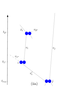
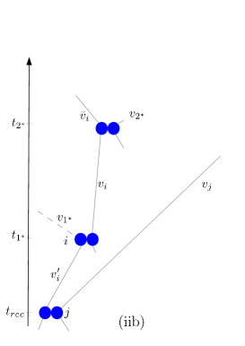
Figure 4. The two collisions at times $t_{1^{*}}$ and $t_{2^{*}}$ leading to the recollision between the pseudo particles $i$ and $j$ are depicted. Three different cases can occur if the first collision involves $i$ : the particle $i$ can be deflected (i), or created without scattering (iia) or with scattering (iib). These three cases can also occur for the recollision at $2^{*}$ but only one is depicted each time.

The condition for the recollision to hold in the backward dynamics at a time $t_{rec}\geq 0$ then states

(3.7) $$(x_{i}-x_{j})+(t_{1^{*}}-t_{2^{*}})(v_{i}-v_{j})+(t_{rec}-t_{1^{*}})(v^{\prime}_{i}-v_{j})={\varepsilon}\nu_{rec}+q\,,$$

for some $\nu_{rec}\in{\mathbb{S}}$, and $q\in\mathbb{Z}^{2}$. As noticed previously, since the total energy is assumed to be bounded by $R^{2}$ and we consider a finite time interval $[0,t]$ with $t\geq 1$, the number of $q$’s for which the set is not empty is at most $O\big{(}R^{2}t^{2}\big{)}$. Let us now fix $q$ and prove that the condition implies that $(t_{1^{*}},v_{1^{*}},\nu_{1^{*}})$ is in a small domain depending only on $x_{i}-x_{j}$, $v_{i}$, $v_{j}$ and $q$.

As previously we consider separately

• the case when the particle $i$ already exists before $t_{1^{*}}$ (as depicted in Figure 4(i)) : the velocity of particle $i$ after $t_{1^{*}}$ (in the backward dynamics) is then

  $(\mathrm{i})$ $$v^{\prime}_{i}=v_{i}-\big{(}(v_{i}-v_{1^{*}})\cdot\nu_{1^{*}}\big{)}\,\nu_{1^{*}}\,.$$

• the case when the particle $i$ was created at $t_{1^{*}}$ : we then get

  $(\mathrm{iia})$ $$v^{\prime}_{i}=v_{1^{*}},$$

  if $(v_{1^{*}},\nu_{1^{*}},v_{i})$ is a precollisional configuration as on Figure 4(iia), and

  $(\mathrm{iib})$ $$v^{\prime}_{i}=v_{1^{*}}+\big{(}(v_{i}-v_{1^{*}})\cdot\nu_{1^{*}}\big{)}\,\nu_{1^{*}}\,,$$

  if $(v_{1^{*}},\nu_{1^{*}},v_{i})$ is a post-collisional configuration as on Figure 4(iib).

We denote

$$\delta x:=\frac{1}{{\varepsilon}}(x_{i}-x_{j}-q)\quad\hbox{ in case (i), and}\quad\delta x:=\frac{1}{{\varepsilon}}(x_{i}-x_{j}-q)+\nu_{1^{*}}\quad\hbox{ in case (ii)}\,.$$

Next we decompose $\delta x$ into a component along $v_{i}-v_{j}$ and an orthogonal component, by writing

$$\delta x={\lambda\over{\varepsilon}}(v_{i}-v_{j})+\delta x_{\perp}\quad\hbox{ with }\quad\delta x_{\perp}\cdot(v_{i}-v_{j})=0\,,$$

and we further rescale time as

(3.8) $$\tau_{1}:=-\frac{1}{{\varepsilon}}(t_{1^{*}}-t_{2^{*}}+\lambda)\,,\qquad\tau_{rec}:=-\frac{1}{{\varepsilon}}(t_{rec}-t_{1^{*}})\,.$$

Note that we have used the hyperbolic scaling invariance (by scaling the space and time variables by ${\varepsilon}$), and that only the bounds on $\tau_{1}$ depend now on ${\varepsilon}$

$$|v_{i}-v_{j}|\,|\tau_{1}|\leq\frac{1}{{\varepsilon}}|v_{i}-v_{j}|t+|\delta x|\leq{CRt\over{\varepsilon}}\,\cdotp$$

We shall gain a factor ${\varepsilon}$ on the integral in time, thanks to the change of variable $t_{1^{*}}\mapsto\tau_{1}$.

In these new variables, the equation for the recollision can be restated as follows

(3.9) $$v^{\prime}_{i}-v_{j}=\frac{1}{\tau_{rec}}\delta x_{\perp}-\frac{\tau_{1}}{\tau_{rec}}(v_{i}-v_{j})-\frac{1}{\tau_{rec}}\nu_{rec}\,.$$

By using (B.4) with $M=R$, we can restrict to the case $|\tau_{1}|\,|v_{i}-v_{j}|\geq R$ so that

$$\big{|}\delta x_{\perp}-\tau_{1}(v_{i}-v_{j})\big{|}\gg 1,$$

as $\delta x_{\perp}\perp(v_{i}-v_{j})$. Since the total energy is bounded by $R^{2}$, the left-hand side of (3.9) is bounded by $2R$, and we get that

(3.10) $$\frac{1}{|\tau_{rec}|}\leq{4R\over|\tau_{1}||v_{i}-v_{j}|}\,\cdotp$$

Given $\delta x_{\perp}$ and $\tau_{1}(v_{i}-v_{j})$, the relation (3.9) forces $v^{\prime}_{i}-v_{j}$ to belong to a rectangle ${\mathcal{R}}(\delta x_{\perp},v_{i}-v_{j},\tau_{1},q)$ of main axis $\delta x_{\perp}-\tau_{1}(v_{i}-v_{j})$ and of size $2R\times\left(2R\min\left(\frac{4}{|\tau_{1}||v_{i}-v_{j}|},1\right)\right)$. The length $2R$ is a consequence of the cut-off on the velocities. The following lemma provides an upper bound on this constraint.

Lemma 3.7.

Fix $t\geq 1$, $\delta x_{\perp}\in\mathbb{R}^{2}$, $v_{i},v_{j}\in B_{R}$ with $1\leq R^{2}\leq C_{0}|\log{\varepsilon}|$, and $1\leq t\leq C_{0}|\log{\varepsilon}|$. Then

$$\int_{B_{R}\times{\mathbb{S}}\times[-Ct/{\varepsilon},Ct/{\varepsilon}]}{\bf 1}_{\{v^{\prime}_{i}-v_{j}\in{\mathcal{R}}(\delta x_{\perp},v_{i}-v_{j},\tau_{1},q)\}}\;\big{|}(v_{1^{*}}-v_{i})\cdot\nu_{{1^{*}}}\big{|}d\tau_{1}d\nu_{1^{*}}dv_{1^{*}}\leq\frac{CR^{3}(\log{\varepsilon})^{2}}{|v_{i}-v_{j}|}\,\cdotp$$

Proof of Lemma 3.7.

Applying (C.10) of Lemma C.4 page C.4, we deduce that

$$\int\!\!{\bf 1}_{\{v^{\prime}_{i}-v_{j}\in{\mathcal{R}}(\delta x_{\perp},v_{i}-v_{j},\tau_{1},q)\}} \big{|}(v_{1^{*}}-v_{i})\cdot\nu_{{1^{*}}}\big{|}\,dv_{1^{*}}d\nu_{1^{*}}$$

$$\leq CR^{3}\min\left(\frac{4}{|\tau_{1}||v_{i}-v_{j}|},1\right)\Big{(}|\log(|\tau_{1}||v_{i}-v_{j}|)|+\log R\Big{)}$$

$$\leq CR^{3}|\log{\varepsilon}|\min\left(\frac{4}{|\tau_{1}||v_{i}-v_{j}|},1\right),$$

recalling that $R^{2}+t\ll|\log{\varepsilon}|$. Integrating with respect to $|v_{i}-v_{j}|\,|\tau_{1}|$ up to $Rt/{\varepsilon}$, we obtain that

$$\int{\bf 1}_{\{v^{\prime}_{i}-v_{j}\in{\mathcal{R}}(\delta x_{\perp},v_{i}-v_{j},\tau_{1},q)\}}\;\,\,\big{|}(v_{1^{*}}-v_{i})\cdot\nu_{{1^{*}}}\big{|}|v_{i}-v_{j}|d\tau_{1}dv_{1^{*}}d\nu_{1^{*}}\leq CR^{3}(\log{\varepsilon})^{2}.$$

This completes Lemma 3.7. ∎

In Lemma 3.7, the measure of the set leading to a recollision is evaluated in terms of the variable $\tau_{1}$. Going back to the variables $(v_{1^{*}},\nu_{1^{*}},t_{1^{*}})$ and summing over all possible $q$, we therefore obtain

(3.11) $$\int{\bf 1}_{\{v^{\prime}_{i}-v_{j}\in\cup_{q}{\mathcal{R}}(\delta x_{\perp},v_{i}-v_{j},\tau_{1},q)\}}\,\,\big{|}(v_{1^{*}}-v_{i})\cdot\nu_{{1^{*}}}\big{|}dt_{1^{*}}dv_{1^{*}}d\nu_{1^{*}}\leq CR^{5}t^{2}{{\varepsilon}|\log{\varepsilon}|^{2}\over|v_{i}-v_{j}|}\,\cdotp$$

On the other hand, a direct computation shows that

$$\int\,\big{|}(v_{1^{*}}-v_{i})\cdot\nu_{{1^{*}}}\big{|}dt_{1^{*}}dv_{1^{*}}d\nu_{1^{*}}\leq CR^{3}t\,,$$

so using the fact that $R\geq 1$, $t\geq 1$, we find

(3.12) $$\int{\bf 1}_{\{v^{\prime}_{i}-v_{j}\in\cup_{q}{\mathcal{R}}(\delta x_{\perp},v_{i}-v_{j},\tau_{1},q)\}}\,\,\big{|}(v_{1^{*}}-v_{i})\cdot\nu_{{1^{*}}}\big{|}dt_{1^{*}}dv_{1^{*}}d\nu_{1^{*}}$$

$$\leq CR^{5}t^{2}\min\Big{(}{{\varepsilon}|\log{\varepsilon}|^{2}\over|v_{i}-v_{j}|}\,,1\Big{)}\,\cdotp$$

Integration of the singularity.

Now we need to integrate out the singularity $1/|v_{i}-v_{j}|$, when the parameters of the preceding collision $(t_{2^{*}},v_{2^{*}},\nu_{2^{*}})$ range over $[0,t]\times B_{R}\times{\mathbb{S}}$. Denote by $\bar{v}_{i}$ the velocity of particle $i$ before the collision with $2^{*}$ (see Figure 4). From (C.1) in Lemma C.1 page C.1, we know that the singularity $1/|v_{i}-v_{j}|$ is integrable if particles $i,j$ are related through the same collision. Otherwise Inequality (C.4), from Lemma C.2, implies that

$$\int\min\Big{(}\frac{{\varepsilon}|\log{\varepsilon}|^{2}}{|v_{j}-v_{i}|},1\Big{)}\,\,\big{|}(v_{2^{*}}-\bar{v}_{i})\cdot\nu_{{2^{*}}}\big{|}dt_{2^{*}}dv_{2^{*}}d\nu_{2^{*}}\leq CtR^{2}{\varepsilon}|\log{\varepsilon}|^{3}\,,$$

and together with (3.12) this implies that

$$\int{\bf 1}_{\{v^{\prime}_{i}-v_{j}\in\cup_{q}{\mathcal{R}}(\delta x_{\perp},v_{i}-v_{j},\tau_{1},q)\}}\prod_{m=1^{*},2^{*}}\,\big{|}\big{(}v_{m}-v_{a(m)}(t_{{m}}))\cdot\nu_{{m}}\big{|}dt_{{m}}d\nu_{{m}}dv_{{m}}\leq CR^{7}t^{3}{\varepsilon}\,|\log{\varepsilon}|^{3}\,.$$

Now we would like to define bad sets which are parametrized only by $(t_{m},v_{m},\nu_{m})$ for $m=1^{*}$ or $m\leq 2^{*}$.

- Suppose that $2^{*}$ is not the parent of $1^{*}$ (which we will refer to as scenario $p=1$). Then by construction $1^{*}$ will branch on one of the labels less than $2^{*}$. There are exactly two particles  $a(1^{*})$ and $a(2^{*})$ associated with the parents of $1^{*},2^{*}$ and the recollision will take place among these four particles. By construction, the choice of parameters for $1^{*},2^{*}$ leading to a recollision of type $p=1$ can be determined only from the configurations of the particles $a(1^{*}),a(2^{*})$ at height $2^{*}-1$.

The bad set associated with the previous scenario (labelled $p=1$) is denoted $\mathcal{P}_{1}(a,1,\{1^{*},2^{*}\})$ and defined as the union of the previous sets. We end up with the estimate

(3.13) $$\int{\bf 1}_{\mathcal{P}_{1}(a,1,\{1^{*},2^{*}\})}\,\,\prod_{m=1^{*},2^{*}}\,\big{|}\big{(}v_{m}-v_{a(m)}(t_{{m}}))\cdot\nu_{{m}}\big{|}dt_{{m}}d\nu_{{m}}dv_{{m}}\leq CR^{7}t^{3}{\varepsilon}\,|\log{\varepsilon}|^{3}\,.$$

- If $2^{*}$ is the parent of $1^{*}$, we have – by definition – a recollision of type $p=2$. Only one particle involved in the recollision is fixed (it can be either $1^{*}$ or $a(1^{*})$) and the second recolliding particle $j$ is just an obstacle which has to be chosen among the particles with label less than $2^{*}$. Note that this obstacle is just transported freely between time $t_{2^{*}}$ and the time of the recollision.

We then define $\mathcal{P}_{1}(a,2,\{1^{*},2^{*}\})$ as the union over all possible choices of $j<2^{*}$ of the previous sets. This leads to the estimate

(3.14) $$\int{\bf 1}_{\mathcal{P}_{1}(a,2,\{1^{*},2^{*}\})}\,\,\prod_{m=1^{*},2^{*}}\,\big{|}\big{(}v_{m}-v_{a(m)}(t_{{m}}))\cdot\nu_{{m}}\big{|}dt_{{m}}d\nu_{{m}}dv_{{m}}\leq CR^{7}st^{3}{\varepsilon}\,|\log{\varepsilon}|^{3}\,.$$

Note that $\mathcal{P}_{1}(a,p,\{1^{*},2^{*}\})$ is empty if the parent of $1^{*}$ has a label greater than $2^{*}$. This ends the proof of the proposition.∎

Remark 3.8.

Estimate (3.4) involves a loss with respect to ${\varepsilon}$ of the order $|\log{\varepsilon}|^{3}$. The above proof shows that the integration in time over the first parent produces a first loss in $|\log{\varepsilon}|^{2}$ (one of which is linked to the scattering operator), while the other power is due to a possible singularity in relative velocities, which needs to be integrated out thanks to the second parent, and the scattering operator again induces a  $|\log{\varepsilon}|$ loss.

3.1.2. Global estimate

To estimate the global error due to recollisions, we have to incorporate the estimate provided in Proposition 3.5 with all the other collision integrals. We use the fact that we have now a tree with $s-2$ or $s-3$ branching points, neglecting the constraints that $(t_{j})_{j\in\sigma}$ have to be properly chosen in between other collision times, and also the constraint on the distribution of collision times on the different time intervals $[t-kh,t-(k-1)h]$.

Proposition 3.9.

We fix $z_{1}\in\mathbb{T}^{2}\times\mathbb{R}^{2}$,  $p\in\{0,1,2\}$ and a set $\sigma\subset\{1,\dots,s\}$ of at most 2 indices. We consider the sets $\mathcal{P}_{1}(a,p,\sigma)$ introduced in Proposition 3.5 and we denote by $\eta:=CsR^{7}t^{3}{\varepsilon}|\log{\varepsilon}|^{3}$ the right-hand side of (3.4). Then for $t\geq 1$, one has

(3.15) $$\sum_{a\in\mathcal{A}_{s}}\int{\bf 1}_{\mathcal{T}_{2,s}}{\bf 1}_{\mathcal{P}_{1}(a,p,\sigma)}\,\Big{(}\prod_{i=2}^{s}\,\big{|}(v_{i}-v_{a(i)}(t_{i}))\cdot\nu_{i}\big{|}\Big{)} M_{\beta}^{\otimes s}\,dT_{2,s}d\Omega_{2,s}dV_{2,s}$$

$$\leq(Ct)^{s-3}s^{2}\eta M_{\beta/2}(v_{1})\,.$$

If we further specify that the last $n$ collision times have to be in an interval of length $h\leq 1$ (this constraint is denoted by $\mathcal{T}_{s-n+1,s}^{h}$)

(3.16) $$\sum_{a\in\mathcal{A}_{s}}\int{\bf 1}_{\mathcal{T}_{2,s}}{\bf 1}_{\mathcal{T}_{s-n+1,s}^{h}}{\bf 1}_{\mathcal{P}_{1}(a,p,\sigma)}\;\Big{(}\prod_{i=2}^{s}\,\big{|}(v_{i}-v_{a(i)}(t_{i}))\cdot\nu_{i}\big{|}\Big{)}M_{\beta}^{\otimes s}\,dT_{2,s}d\Omega_{2,s}dV_{2,s}$$

$$\leq(Ct)^{s-n-1}(Ch)^{n-2}s^{2}\eta M_{\beta/2}(v_{1})\,.$$

Proof.

We only consider the cases $p=1,2$ which are the most delicate. Proposition 3.9 is a consequence of the estimates on the collision operators (see Proposition 2.5) for the particles which are not in $\sigma$ and the smallness estimate (3.4) for the particles in $\sigma$. These estimates can be decoupled by using Fubini’s theorem and the fact that the sets $\mathcal{P}_{1}(a,z_{1},\sigma)$ do not depend on the whole trajectory but only on the parameters with labels less than $2^{*}$ as well as on the parameters associated with $1^{*}$.

In order to evaluate (3.15), we first perform the integration with respect to all the velocities and angles with labels larger than $2^{*}$ except those of the particle $1^{*}$. Recall that $\mathcal{P}_{1}(a,z_{1},\sigma)$ is independent of these parameters. We can use the same estimates as in the proof of Proposition 2.5

$$\sum_{(a(j))_{j>2^{*}\atop j\not\in 1^{*}}}\left(\prod_{i>2^{*},\atop i\not=1^{*}}\,\big{|}(v_{i}-v_{a(i)}(t_{i}))\cdot\nu_{i}\big{|}\right)M_{\beta/4}^{\otimes s}(V_{s})\leq(Cs)^{s-2^{*}-2}\,.$$

and integrate over each label in $\tilde{\sigma}=\{i>2^{*},\quad i\not=1^{*}\}$

(3.17) $$\sum_{(a(j))_{j\in\tilde{\sigma}}}\int\left(\prod_{i\in\tilde{\sigma}}\,\big{|}(v_{i}-v_{a(i)}(t_{i}))\cdot\nu_{i}\big{|}\right)M_{\beta}^{\otimes s}(V_{s})dV_{\tilde{\sigma}}d\Omega_{\tilde{\sigma}}\leq(Cs)^{s-2^{*}-2}M_{3\beta/4}^{\otimes{2^{*}}}(V_{2^{*}})\,.$$

This bound takes into account the combinatorics of the trees up to $2^{*}$. Note that the upper bound (3.17) overestimates (3.15) as we are also counting trees for which the branchings in between $2^{*}$ and $1^{*}$ may not be compatible with the conditions imposed by a recollision. This does not matter as the constraint on the recollision has already been encoded in $\mathcal{P}_{1}(a,z_{1},\sigma)$ which we will use next.

The previous step removed all the dependency on the collision trees below the level $2^{*}$ and we can now use estimate (3.4) and integrate over $1^{*},2^{*}$ (keeping frozen the parameters of the labels before $2^{*}$)

$$\sum_{a(1^{*}),a(2^{*})}\int{\bf 1}_{\mathcal{P}_{1}(a,p,\sigma)}\left(\prod_{i\in\sigma}\,\big{|}(v_{i}-v_{a(i)}(t_{i}))\cdot\nu_{i}\big{|}\right)dT_{\sigma}dV_{\sigma}d\Omega_{\sigma}\leq s^{2}\eta\,,$$

uniformly with respect to all parameters $(t_{i},v_{i},\nu_{i})_{i<2^{*}}$. The factor $s^{2}$ in the inequality comes from the choices of $a(1^{*}),a(2^{*})$.

Once the constraint on the recollision has been taken into account, the remaining part of the tree before $2^{*}$ can be estimated by using the estimates from Proposition 2.5. This leads to an extra factor $(Cs)^{2^{*}-1}$.

It remains to integrate over the times $(t_{i})_{i\not\in\sigma}$ and we can simply remove the constraint on the times labelled by $\sigma$. We distinguish two cases :

• In (3.15), the time constraint $\mathcal{T}_{2,s}$ boils down to integrating over a simplex of dimension $(s-1)-2$, the volume of which is

  $${t^{s-3}\over(s-3)!}\leq C^{s}{t^{s-3}\over s^{s-3}}$$

  by Stirling’s formula.

• In (3.16), we have to add the condition that the last $n$ times are in an interval of length $h\leq 1$. For $t\geq 1$, the worst situation is when all times $(t_{i})_{i\in\sigma}$ are in this small time interval, as we loose the corresponding smallness. More precisely, we get

  $${t^{s-1-n}\over(s-1-n)!}{h^{n-2}\over(n-2)!}\leq C^{s}{t^{s-1-n}h^{n-2}\over s^{s-1-2}}\,\cdotp$$

This completes the proof of Proposition 3.9. ∎

Proof of Proposition 3.2.

Given $z_{1}\in\mathbb{T}^{2}\times B_{R}$, the set of parameters leading to pseudo-trajectories with at least one recollision is partitioned into subsets $\mathcal{P}_{1}(a,p,{\sigma})$ (see Proposition 3.5). We therefore have

(3.18) $$\Big{|} f^{(1,K),\geq}_{N}(t,z_{1})\Big{|}\leq\sum_{j_{1}=0}^{n_{1}-1}\!\!\dots\!\!\sum_{j_{K}=0}^{n_{K}-1}\alpha^{J_{K}-1}\sum_{a\in\mathcal{A}_{J_{K}}}\sum_{p,\sigma}\int{\bf 1}_{\mathcal{T}_{2,J_{k}}}{\bf 1}_{\mathcal{P}_{1}(a,p,\sigma)}$$

$$\quad\times\left(\prod_{i=2}^{J_{K}}\,\big{|}(v_{i}-v_{a(i)}(t_{i}))\cdot\nu_{i}\big{|}\right)\big{(}f^{(J_{K})}_{N,0}{\bf 1}_{{\mathcal{V}}_{J_{K}}}\big{)}\,dT_{2,J_{K}}d\Omega_{2,J_{K}}dV_{2,J_{K}}\,.$$

We have seen in (2.16) that the marginals of the initial datum are dominated by a Maxwellian

$$\big{|}f_{N,0}^{(J_{K})}(Z_{J_{K}})\big{|}\leq C^{J_{K}}M_{\beta}^{\otimes J_{K}}(V_{J_{K}})\|g_{\alpha,0}\|_{L^{\infty}}\,.$$

Thus (3.15) can be applied to estimate $f^{(1,K),\geq}_{N}$

$$\Big{|}f^{(1,K),\geq}_{N}(t,z_{1})\Big{|}\leq\|g_{\alpha,0}\|_{L^{\infty}}\sum_{j_{1}=0}^{n_{1}-1}\!\!\dots\!\!\sum_{j_{K}=0}^{n_{K}-1}C^{J_{K}}\alpha^{J_{K}-1}J_{K}^{5}t^{J_{K}}{\varepsilon}\big{|}\log{\varepsilon}\big{|}^{\frac{19}{2}}M_{\beta/2}(v_{1})\,,$$

where the parameter $\eta$ in (3.15) has been estimated by using that $1\leq R^{2}\leq C_{0}|\log{\varepsilon}|$ and $1\leq t\leq C_{0}|\log{\varepsilon}|$. Note that compared to (3.15), an extra factor $J_{K}^{2}$ was added to take into account the sum over the possible choices for $\sigma$.

Now recalling that $n_{k}=2^{k}n_{0}$ we have

(3.19) $$J_{K}\leq 2^{K+1}n_{0}\quad\text{and}\quad\sum_{j_{1}=0}^{n_{1}-1}\!\!\dots\!\!\sum_{j_{K}=0}^{n_{K}-1}\leq\prod_{i=1}^{K}n_{i}\leq n_{0}^{K}2^{K^{2}}\,,$$

so thanks to Assumption (1.20) on the initial datum $g_{\alpha,0}$, we conclude

$$\Big{|}f^{(1,K),\geq}_{N}(t,z_{1})\Big{|}\leq\exp(C\alpha^{2})2^{4K^{2}}n_{0}^{5+K}\big{(}CT\alpha\big{)}^{2^{K+1}n_{0}}{\varepsilon}\big{|}\log{\varepsilon}\big{|}^{\frac{19}{2}}M_{\beta/2}(v_{1})\,.$$

Since $2^{K^{2}}n_{0}^{5+K}\ll C^{2^{K}}$, this completes the proof of Proposition 3.2 (bounding $\big{|}\log{\varepsilon}\big{|}^{\frac{19}{2}}$ by $\big{|}\log{\varepsilon}\big{|}^{10}$ to simplify). ∎

3.2. Proof of Proposition 3.1

Each term in the decomposition (3.3)

$$f^{(1,K)}_{N}(t)=f^{(1,K),0}_{N}(t)+f^{(1,K),\geq}_{N}(t)$$

can be interpreted as a restriction of the domain of integration of the times, velocities and deflection angles. For $f^{(1,K),\geq}_{N}$, the pseudo-trajectories associated with a tree $a$ are integrated over the sets $\mathcal{P}_{1}(a,p,\sigma)$ as in (3.18), instead they are integrated outside these sets in $f^{(1,K),0}_{N}$. As a consequence the pseudo-trajectories in $f^{(1,K),0}_{N}$ have no recollision.

A similar decomposition holds for the Boltzmann hierarchy: we distinguish whether the pseudo-trajectories lie on the non-overlapping sets $G_{s}(a)$ or not (see Definition 2.3), and whether they lie on the pathological sets $\mathcal{P}_{1}(a,p,\sigma)$ or not (this splitting is artificial as there are no recollisions in the Boltzmann hierarchy, however it will be useful to compare the different contributions). Recalling

$$\bar{f}^{(1,K)}(t):=\sum_{j_{1}=0}^{n_{1}-1}\!\!\dots\!\!\sum_{j_{K}=0}^{n_{K}-1}\bar{Q}_{1,J_{1}}(h)\bar{Q}_{J_{1},J_{2}}(h)\dots\bar{Q}_{J_{K-1},J_{K}}(h)\,\big{(}f^{(J_{K})}_{0}{\bf 1}_{{\mathcal{V}}_{J_{K}}}\big{)}\,,$$

let us write

$$\bar{f}^{(1,K)}=\bar{f}^{(1,K),0}+\bar{f}^{(1,K),\geq}+\bar{f}^{(1,K),\rm{overlap}}\,,$$

where $\bar{f}^{(1,K),0}(t)$ corresponds to restricting the pseudo-trajectories to the sets of parameters ${}^{c}{}\mathcal{P}_{1}(a,p,\sigma)\cap G_{s}(a)$, while $\bar{f}^{(1,K),\geq}(t)$ corresponds to the restriction to $\mathcal{P}_{1}(a,p,\sigma)\cap G_{s}(a)$, and finally $\bar{f}^{(1,K),\rm{overlap}}(t)$ corresponds to the restriction to ${}^{c}{}G_{s}(a)$. As a consequence of Proposition 3.2, the term $\bar{f}^{(1,K),\geq}$ is negligible

(3.20) $$\Big{|}\bar{f}^{(1,K),\geq}(t,z_{1})\Big{|}\leq\exp(C\alpha^{2})\big{(}CT\alpha\big{)}^{2^{K+1}n_{0}}{\varepsilon}\big{|}\log{\varepsilon}\big{|}^{10}M_{\beta/2}(v_{1})\,.$$

Similarly we claim that

(3.21) $$\Big{|}\bar{f}^{(1,K),\rm{overlap}}(t,z_{1})\Big{|}\leq\exp(C\alpha^{2})\big{(}CT\alpha\big{)}^{2^{K+1}n_{0}}{\varepsilon}\big{|}\log{\varepsilon}\big{|}^{10}M_{\beta/2}(v_{1})\,.$$

Indeed we notice that by definition

$${}^{c}{}G_{s}\subset\widetilde{{}^{c}{}G_{s}}:=\Big{\{}(T_{2,s},\Omega_{2,s},V_{2,s})\in\mathcal{T}_{2,s}\times{\mathbb{S}}^{s-1}\times\mathbb{R}^{2(s-1)}\,/\,\exists i\,,\,\exists k,\ell<i\,/\,|x_{k}(t_{i})-x_{\ell}(t_{i})|\leq 2{\varepsilon}\Big{\}}\,.$$

If $(T_{2,s},\Omega_{2,s},V_{2,s})$ belongs to $\widetilde{{}^{c}{}G_{s}}$ and if $i$ is the smallest integer such that

(3.22) $$\exists k,\ell<i\,/\,|x_{k}(t_{i})-x_{\ell}(t_{i})|\leq 2{\varepsilon}\,,$$

then either the corresponding pseudotrajectory before time $t_{i}$ (which exists by definition of $i$) has suffered at least one recollision, and the result is a consequence of the proof of Proposition  3.2; or the condition (3.22) can itself be interpreted as a “recollision” (with ${\varepsilon}$ replaced by $2{\varepsilon}$) and the computations leading to Proposition 3.2 may again be reproduced exactly. So (3.21) follows.

The last step to conclude Proposition 3.1 is to evaluate the difference $f^{(1,K),0}_{N}(t)-\bar{f}^{(1,K),0}(t)$. Once recollisions and overlaps have been excluded, the only discrepancies between the BBGKY and the Boltzmann pseudo-trajectories come from the micro-translations due to the diameter ${\varepsilon}$ of the colliding particles (see Definition 2.2). At the initial time, the error between the two configurations is at most $O(s{\varepsilon})$ after $s$ collisions (see [9, 5])

(3.23) $$\big{|}\bar{X}_{s}(a,T_{2,s},\Omega_{2,s},V_{2,s},0)-X_{s}(a,T_{2,s},\Omega_{2,s},V_{2,s},0)\big{|}\leq Cs{\varepsilon}\,.$$

The discrepancies are only for positions, as velocities remain equal in both hierarchies. These configurations are then evaluated either on the marginals of the initial datum $f_{N,0}^{(s)}$ or of $f^{(s)}_{0}$ which are close to each other thanks to Proposition 2.6.

The main discrepancy between $f^{(1,K),0}_{N}$ and $\bar{f}^{(1,K),0}$ depends on

$$\Big{|}f_{0}^{(s)}\Big{(}\bar{Z}_{s}(a,T_{2,s},\Omega_{2,s},V_{2,s},0)\Big{)}-f_{N,0}^{(s)}\Big{(}Z_{s}(a,T_{2,s},\Omega_{2,s},V_{2,s},0)\Big{)}\Big{|}$$

$$\qquad\leq\Big{|}f_{0}^{(s)}\Big{(}\bar{Z}_{s}(a,T_{2,s},\Omega_{2,s},V_{2,s},0)\Big{)}-f_{0}^{(s)}\Big{(}Z_{s}(a,T_{2,s},\Omega_{2,s},V_{2,s},0)\Big{)}\Big{|}$$

$$\qquad\qquad+\Big{|}f_{0}^{(s)}\Big{(}Z_{s}(a,T_{2,s},\Omega_{2,s},V_{2,s},0)\Big{)}-f_{N,0}^{(s)}\Big{(}Z_{s}(a,T_{2,s},\Omega_{2,s},V_{2,s},0)\Big{)}\Big{|}\,.$$

By the assumption (1.20), $g_{\alpha,0}$ has a Lipschitz bound $\exp(C\alpha^{2})$, thus combining (3.23) and the estimate of Proposition 2.6, we get

$$\Big{|}f_{0}^{(s)}\Big{(}\bar{Z}_{s}(a,T_{2,s},\Omega_{2,s},V_{2,s},0)\Big{)}-f_{N,0}^{(s)}\Big{(}Z_{s}(a,T_{2,s},\Omega_{2,s},V_{2,s},0)\Big{)}\Big{|}\leq C^{s}\exp(C\alpha^{2})s{\varepsilon}M_{\beta}^{\otimes s}(V_{s})\,.$$

The last source of discrepancy between the formulas defining $f^{(1,K),0}_{N}$ and $\bar{f}_{N}^{(1,K),0}$ comes from the prefactor $(N-1)\dots(N-s+1){\varepsilon}^{s-1}$ which has been replaced by $\alpha^{s-1}$. For fixed $s$, the corresponding error is

$$\Big{(}1-{(N-1)\dots(N-s+1)\over N^{s-1}}\Big{)}\leq C{s^{2}\over N}\leq Cs^{2}{{\varepsilon}\over\alpha}$$

which, combined with the bound on the collision operators, leads to an error of the form

(3.24) $$(C\alpha t)^{s-1}s^{2}{{\varepsilon}\over\alpha}\,\cdotp$$

Summing the previous bounds gives

(3.25) $$\Big{|}f^{(1,K),0}_{N}(t,z_{1})-\bar{f}^{(1,K),0}(t,z_{1})\Big{|} \leq\exp(C\alpha^{2})M_{\beta}(v_{1})\sum_{j_{1}=0}^{n_{1}-1}\!\!\dots\!\!\sum_{j_{K}=0}^{n_{K}-1}(C\alpha t)^{J_{K}-1}\left(J_{K}^{2}\,{{\varepsilon}\over\alpha}+J_{K}{\varepsilon}\right)$$

$$\leq\exp(C\alpha^{2})M_{\beta}(v_{1})\big{(}CT\alpha\big{)}^{2^{K+1}n_{0}}\left(2^{2(K+1)}\,{{\varepsilon}\over\alpha}+2^{K+1}{\varepsilon}\right),$$

where we used the bounds (3.19) for the sequence $n_{k}=2^{k}n_{0}$ .

Finally Proposition 3.1 follows by combining

• Proposition 3.2 and (3.20) to control the recollisions,

• (3.21) to control overlaps in the pseudo-trajectories,

• (3.25) to control the difference in the parts without recollisions.

The result is proved. ∎

4. Symmetry and $L^{2}$ bounds

In this section, we prove an upper bound on the contribution of super exponential collision trees without recollisions introduced in (2.26)

$$R_{N}^{K,0}(t):=\sum_{k=1}^{K}\sum_{j_{i}<n_{i}\atop i\leq k-1}\sum_{j_{k}\geq n_{k}}Q^{0}_{1,J_{1}}(h)\dots Q^{0}_{J_{k-1},J_{k}}(h)\big{(}f^{(J_{K})}_{N}(t-kh){\bf 1}_{{\mathcal{V}}_{J_{K}}}\big{)}\,.$$

Proposition 4.1.

Given $T>1$, $\gamma\ll 1$ and $C$ a large enough constant (independent of $\gamma$ and $T$), the parameters are tuned as follows

(4.1) $$h\leq{\gamma^{2}\over\exp(C\alpha^{2})T^{3}}\,,\qquad n_{k}=2^{k}n_{0}\,.$$

Then, under the Boltzmann-Grad scaling $N{\varepsilon}=\alpha\gg 1$, we have for $t\in[0,T]$

(4.2) $$\Big{\|}R_{N}^{K,0}(t)\Big{\|}_{L^{2}(\mathbb{D})}\leq\gamma\,.$$

The main step to derive Proposition 4.1 is to replace the $L^{\infty}$ estimates on the collision kernel (Proposition 2.5) by $L^{2}$ estimates. To do this, we first establish an $L^{2}_{\beta}$ decomposition of the marginals $f_{N}^{(s)}(t)$ (Proposition 4.2 in Section 4.1) and then an $L^{2}$ counterpart of Proposition 2.5 (Proposition 4.4 in Section 4.2).

4.1. Structure of symmetric functions in $L^{2}$

We prove in Proposition 4.2 that a structure similar to (2.20) is intrinsic to symmetric functions with suitable $L^{2}$ bounds (the argument does not involve dynamics). As the density $f_{N}(t)$ of the particle system is symmetric and admits $L^{2}$ bounds uniform in time, we can then deduce that the higher order correlations of the marginals $f_{N}^{(s)}(t,Z_{s})$ are small in $L^{2}$ for any time. This is a key ingredient in the proof of the main theorem.

The following proposition states a general decomposition of symmetric functions in $L^{2}_{\beta}$.

Proposition 4.2.

Let $f_{N}$ be a mean free, symmetric function such that $f_{N}/M_{\beta}^{\otimes N}\in L^{2}_{\beta}(\mathbb{D}^{N})$. There exist symmetric functions $g_{N}^{m}$ on $\mathbb{D}^{m}$ for $1\leq m\leq N$ such that for all $s\leq N$, the marginal of order $s$ satisfies

(4.3) $$f_{N}^{(s)}(Z_{s})=M_{\beta}^{\otimes s}(V_{s})\sum_{m=1}^{s}\sum_{\sigma\in{\mathfrak{S}}^{m}_{s}}g_{N}^{{m}}(Z_{\sigma})\,,$$

where ${\mathfrak{S}}^{m}_{s}$ denotes the set of all parts of $\{1,\dots,s\}$ with $m$ elements, and $\binom{N}{m}$ is its cardinal. Moreover

$$\|g_{N}^{m}\|^{2}_{L^{2}_{\beta}(\mathbb{D}^{m})}\leq{{1\over\binom{N}{m}}}\|f_{N}/M_{\beta}^{\otimes N}\|^{2}_{L^{2}_{\beta}(\mathbb{D}^{N})}\,.$$

Combining (2.17) and (2.19), we see that at any time $t\geq 0$

(4.4) $$\int{f_{N}^{2}\over M_{\beta}^{\otimes N}}(t,Z_{N})dZ_{N}\leq\frac{1}{{\mathcal{Z}}_{N}}\int{f_{N}^{2}\over M_{N,\beta}}(t,Z_{N})dZ_{N}\leq CN\exp(C\alpha^{2})\|g_{\alpha,0}\|_{L^{2}_{\beta}(\mathbb{D})}^{2}\,.$$

Thus Proposition 4.2 applies to the solution $f_{N}(t)$ of the Liouville equation and for all $s\leq N$, the marginal of order $s$ satisfies

(4.5) $$f_{N}^{(s)}(t,Z_{s})=M_{\beta}^{\otimes s}(V_{s})\sum_{m=1}^{s}\sum_{\sigma\in{\mathfrak{S}}^{m}_{s}}g_{N}^{{m}}(t,Z_{\sigma})\,,$$

with

(4.6) $$\forall t\geq 0,\qquad\|g_{N}^{m}(t)\|^{2}_{L^{2}_{\beta}(\mathbb{D}^{m})}\leq{CN\exp(C\alpha^{2})\over\binom{N}{m}}\|g_{\alpha,0}\|_{L^{2}_{\beta}(\mathbb{D})}^{2}\,.$$

Although the definition is not exactly the usual one (due to the linear setting), we will call cumulant of order $m$ the function $g_{N}^{m}$ as it encodes the correlations of order $m$. It is indeed defined by some exhaustion procedure (which is somehow comparable to the Calderón-Zygmund decomposition), which ensures that the average of $g_{N}^{m}$ with respect to any of its coordinate is zero. In other words, all correlations of order less than $m-1$ have been removed.

Note that the size of the correlations between several particles has been quantified by Pulvirenti, Simonella [23] for chaotic initial data. As in (4.6), the bounds obtained in [23] decrease with the degree of the correlations, however these estimates hold only for short times and moderate $m$ as they are valid even far from equilibrium.

The decomposition (4.5) can be understood as a projection of $f_{N}$ onto the reference measure $M_{\beta}^{\otimes N}$ and the terms in (4.6) are small because $f_{N}$ is close to $M_{\beta}^{\otimes N}$ in the $L^{2}$ sense (4.4). In $d\geq 3$, the estimate (4.4) no longer holds (even for $f_{N}=M_{N,\beta}$) as the corrections induced by the exclusion are too large. Thus to generalize the previous decomposition in $d\geq 3$, one would need to replace the reference measure $M_{\beta}^{\otimes N}$ by a more suitable one.

Proof of Proposition 4.2.

Define

$$g_{N}^{m}(Z_{m}):=\sum_{k=1}^{m}(-1)^{m-k}\sum_{{\sigma}\in{\mathfrak{S}}_{m}^{k}}{f_{N}^{(k)}\over M_{\beta}^{\otimes k}}(Z_{\sigma})\,.$$

Step 1. The identity

(4.7) $${f_{N}\over M_{\beta}^{\otimes N}}(Z_{N})=\sum_{m=1}^{N}\sum_{{\sigma}\in{\mathfrak{S}}_{N}^{m}}g_{N}^{m}(Z_{\sigma})$$

comes from a simple application of Fubini’s theorem. We indeed have

$$\sum_{m=1}^{N}\sum_{{\sigma}\in{\mathfrak{S}}_{N}^{m}}g_{N}^{m}(Z_{\sigma}) =\sum_{m=1}^{N}\sum_{{\sigma}\in{\mathfrak{S}}_{N}^{m}}\sum_{k=1}^{m}(-1)^{m-k}\sum_{{\tilde{\sigma}}\in{\mathfrak{S}}_{m}^{k}}{f_{N}^{(k)}\over M_{\beta}^{\otimes k}}(Z_{\tilde{\sigma}})$$

$$=\sum_{k=1}^{N}\sum_{{\tilde{\sigma}}\in{\mathfrak{S}}_{N}^{k}}{f_{N}^{(k)}\over M_{\beta}^{\otimes k}}(Z_{\tilde{\sigma}})\sum_{m=k}^{N}(-1)^{m-k}\binom{N-k}{m-k},$$

since the number of possible $\sigma$ with $m$ elements having $\tilde{\sigma}$ as a subset is $\binom{N-k}{m-k}$.

For $k<N$, we have

$$\sum_{m=k}^{N}(-1)^{m-k}\binom{N-k}{m-k}=\sum_{m=0}^{N-k}(-1)^{m}\binom{N-k}{m}=0^{N-k}=0\,,$$

while for $k=N$ we just obtain 1. We therefore get (4.7).

Step 2. We prove now that

(4.8) $$\int g_{N}^{m}(Z_{m})M_{\beta}(v_{\ell})\,dz_{\ell}=0\,,\quad 1\leq\ell\leq m\,.$$

Given $1\leq\ell\leq m$, one can split the sum over ${\sigma}\in{\mathfrak{S}}_{m}^{k}$ into two pieces, depending on whether $\ell$ belongs to ${\sigma}$ or not

$$\int g_{N}^{m}(Z_{m})M_{\beta}(v_{\ell})\,dz_{\ell}$$

$$\quad=\sum_{k=1}^{m}(-1)^{m-k}\sum_{\scriptstyle{{\sigma}\in{\mathfrak{S}}_{m}^{k}}\atop\scriptstyle{\ell\in{\sigma}}}\int{f_{N}^{(k)}\over M_{\beta}^{\otimes k}}(Z_{\sigma})M_{\beta}(v_{\ell})dz_{\ell}+\sum_{k=1}^{m-1}(-1)^{m-k}\sum_{\scriptstyle{{\sigma}\in{\mathfrak{S}}_{m}^{k}}\atop\scriptstyle{\ell\notin{\sigma}}}\int{f_{N}^{(k)}\over M_{\beta}^{\otimes k}}(Z_{\sigma})M_{\beta}(v_{\ell})dz_{\ell}$$

$$\quad=\sum_{k^{\prime}=0}^{m-1}(-1)^{m-k^{\prime}+1}\sum_{{\sigma}\in{\mathfrak{S}}_{m-1}^{k^{\prime}}\atop\ell\notin{\sigma}}{f_{N}^{(k^{\prime})}\over M_{\beta}^{\otimes k^{\prime}}}(Z_{\sigma})+\sum_{k=1}^{m-1}(-1)^{m-k}\sum_{\scriptstyle{{\sigma}\in{\mathfrak{S}}_{m}^{k}}\atop\scriptstyle{\ell\notin{\sigma}}}{f_{N}^{(k)}\over M_{\beta}^{\otimes k}}(Z_{\sigma})\,.$$

The conclusion follows from the fact that the case $k^{\prime}=0$ corresponds to

$$\int{f_{N}^{(1)}\over M_{\beta}}(z_{\ell})M_{\beta}(v_{\ell})dz_{\ell}=\int f_{N}(Z_{N})dZ_{N}=0\,.$$

Hence we obtain

$$\int g_{N}^{m}(Z_{m})M_{\beta}(v_{\ell})\,dz_{\ell}=0\,.$$

The identity (4.3) follows by integrating (4.7) with respect to $M_{\beta}^{\otimes(N-s)}dz_{s+1}\dots dz_{N}$

$$f_{N}^{(s)}(Z_{s})=M_{\beta}^{\otimes s}\sum_{m=1}^{s}\sum_{\sigma\in{\mathfrak{S}}^{m}_{s}}g_{N}^{m}(Z_{\sigma})\,.$$

Step 3. It remains to establish estimate (4.6). From (4.7) and the orthogonality condition (4.8), we also deduce that

$$\int{f_{N}^{2}\over M^{\otimes N}_{\beta}}dZ_{N} =\int M_{\beta}^{\otimes N}\left(\sum_{m=1}^{N}\sum_{{\sigma}\in{\mathfrak{S}}_{N}^{m}}g_{N}^{m}(Z_{\sigma})\right)^{2}dZ_{N}=\sum_{m=1}^{N}\sum_{{\sigma}\in{\mathfrak{S}}_{N}^{m}}\int M_{\beta}^{\otimes N}\left(g_{N}^{m}(Z_{\sigma})\right)^{2}dZ_{N}$$

$$=\sum_{m=1}^{N}\binom{N}{m}\|g_{N}^{m}\|^{2}_{L^{2}_{\beta}(\mathbb{D}^{m})}\,.$$

This ends the proof of Proposition 4.2. ∎

Remark 4.3.

The decomposition (4.3) shows that the higher order correlations decrease in $L^{2}$-norm according to the number of particles. This is a step towards proving local equilibrium, but these estimates are not strong enough to deduce directly that the equation on the first marginal can be closed because the collision operator is too singular.

4.2. $L^{2}$ continuity estimates for the iterated collision operators

We will now establish an $L^{2}$ estimate for $Q^{0}_{1,J}(t)$ (see Proposition 4.4). As explained in the introduction (see Paragraph 2.5), it involves a loss in ${\varepsilon}$, which will be exactly compensated by the decay of the $L^{2}_{\beta}$-norm (4.6) in the expansion (4.3). This shows that the structure (2.20) is partly preserved by the collision-transport operators, as long as there is no recollision.

4.2.1. Statement of the result and strategy of the proof

Let us first introduce some notation. As in (2.7) for $|Q_{s,s+n}|(t)$, the operator $|Q^{0}_{s,s+n}|(t)$ is obtained by considering the sum $C^{+}_{s,s+1}+C^{-}_{s,s+1}$ instead of the difference. Let $g_{m}\in L^{2}_{\beta}(\mathbb{D}^{m})$, we set for ${\sigma}\in{\mathfrak{S}}_{s}^{m}$

(4.9) $$g_{m,\sigma}(Z_{s})=g_{m}(Z_{\sigma})\,.$$

The key estimate is given by the following proposition. Note that the bound provided in (4.10) is not the best one can prove (in terms of the way the powers of $t$ and $h$ are divided) but suffices for our purposes.

Proposition 4.4.

There is a constant $C$ (depending only on $\beta$) such that for all $J,n\in\mathbb{N}^{*}$ and all $t\geq 1,h\in[0,t]$, the operator $|Q^{0}|$ satisfies the following continuity estimate

(4.10) $$\Big{\|}|Q_{1,J}^{0}|(t)\,|Q^{0}_{J,J+n}|(h)\,\sum_{\sigma\in{\mathfrak{S}}^{m}_{J+n}}{{\bf 1}_{{\mathcal{V}}_{J+n}}}M_{\beta}^{\otimes(J+n)}\big{|}g_{m,\sigma}\big{|}\Big{\|}_{L^{2}(\mathbb{D})}$$

$$\qquad\qquad\qquad\qquad\qquad\leq(C\alpha)^{J+n-1}t^{J+n/2-1}h^{n/2}{\|g_{m}\|_{L^{2}_{\beta}(\mathbb{D}^{m})}\over\sqrt{{\varepsilon}^{m-1}m!}}\,\cdotp$$

Proof.

To simplify the analysis, especially the treatment of large velocities, we define modified collision operators

(4.11) $$\big{(}C^{b,\pm}_{s,s+1}h^{s+1}\big{)}(Z_{s}):=\frac{(N-s){\varepsilon}}{\alpha}\sum_{i=1}^{s} \int_{{\mathbb{S}}\times\mathbb{R}^{2}}h^{s+1}(Z_{s+1}^{\pm,i,s+1}){\big{(}(v_{i}-v_{s+1})\cdot\nu\big{)}_{+}\over 1+|v_{i}-v_{s+1}|}\,d\nu dv_{s+1}\,,$$

$$\big{(}C^{q,\pm}_{s,s+1}h^{s+1}\big{)}(Z_{s}):=\frac{(N-s){\varepsilon}}{\alpha}\sum_{i=1}^{s} \int_{{\mathbb{S}}\times\mathbb{R}^{2}}h^{s+1}(Z_{s+1}^{\pm,i,s+1})$$

$$\qquad\times(1+|v_{i}-v_{s+1}|){\big{(}(v_{i}-v_{s+1})\cdot\nu\big{)}_{+}}\,d\nu dv_{s+1},$$

where $Z_{s+1}^{\pm,i,s+1}$ denotes the configuration after the collision between $i$ and $s+1$ as in (1.9)

$$Z_{s+1}^{-,i,s+1} :=(x_{1},v_{1},\dots,x_{i},v_{i},\dots,x_{i}-{\varepsilon}\nu,v_{s+1})\,,$$

$$Z_{s+1}^{+,i,s+1} :=(x_{1},v_{1},\dots,x_{i},v_{i}^{\prime},\dots,x_{i}+{\varepsilon}\nu,v_{s+1}^{\prime})\,.$$

By construction, $C^{b,\pm}_{s,s+1}$ has a bounded collision cross-section and $C^{q,\pm}_{s,s+1}$ has a collision cross-section with quadratic growth in $v$. Defining accordingly $|Q^{b,0}_{1,J}|$ and $|Q^{q,0}_{1,J}|$, we have by the Cauchy-Schwarz inequality

$$\Big{|}\,|Q_{1,J}^{0}|(t)\,|Q^{0}_{J,J+n}|(h) \sum_{\sigma\in{\mathfrak{S}}^{m}_{J+n}}M_{\beta}^{\otimes(J+n)}{{\bf 1}_{{\mathcal{V}}_{J+n}}}\big{|}g_{m,\sigma}\big{|}\Big{|}$$

$$\leq\Big{(}\sum_{\sigma\in{\mathfrak{S}}^{m}_{J+n}}|Q_{1,J}^{q,0}|(t)\,|Q^{q,0}_{J,J+n}|(h)\,M_{\beta}^{\otimes(J+n)}\Big{)}^{1/2}$$

$$\qquad\times\Big{(}|Q_{1,J}^{b,0}|(t)\,|Q^{b,0}_{J,J+n}|(h)\sum_{\sigma\in{\mathfrak{S}}^{m}_{J+n}}M_{\beta}^{\otimes(J+n)}g_{m,\sigma}^{2}\Big{)}^{1/2},$$

where the velocity cut-off ${\mathcal{V}}_{J+n}$ has been dropped. Thus we find directly

(4.12) $$\Big{|}\,|Q_{1,J}^{0}|(t)\,|Q^{0}_{J,J+n}|(h) \sum_{\sigma\in{\mathfrak{S}}^{m}_{J+n}}M_{\beta}^{\otimes(J+n)}\big{|}g_{m,\sigma}\big{|}\Big{|}$$

$$\leq 2^{\frac{J+n}{2}}\Big{(}|Q_{1,J}^{q,0}|(t)\,|Q^{q,0}_{J,J+n}|(h)\,M_{\beta}^{\otimes(J+n)}\Big{)}^{1/2}$$

$$\qquad\times\Big{(}|Q_{1,J}^{b,0}|(t)\,|Q^{b,0}_{J,J+n}|(h)\,\sum_{\sigma\in{\mathfrak{S}}^{m}_{J+n}}M_{\beta}^{\otimes(J+n)}g_{m,\sigma}^{2}\Big{)}^{1/2}\,.$$

$\bullet$ The first factor can be bounded in $L^{\infty}$ as in Proposition 2.5.

Proposition 4.5.

There is a constant $C$ (depending only on $\beta$) such that for all $J,n\in\mathbb{N}^{*}$ and all $h,t\geq 0$, the operator $|Q^{q,0}|$ satisfies the following continuity estimates

(4.13) $$\forall z_{1}\in\mathbb{D}\,,\qquad|Q_{1,J}^{q,0}|(t)\,|Q_{J,J+n}^{q,0}|(h)M_{\beta}^{\otimes(J+n)}(z_{1})\leq(C\alpha t)^{J-1}(C\alpha h)^{n}M_{3\beta/4}(z_{1})\,.$$

The proof is omitted as it is similar to the one of Proposition 2.5 (we just have to skip the Cauchy-Schwarz estimate in (2.9)). Note that the quadratic growth in the collision cross-section is critical in the sense that it is the highest possible power giving an admissible loss estimate.

Thus (4.12) can be bounded as follows

(4.14) $$\int_{\mathbb{D}}\Big{(}\,|Q_{1,J}^{0}|(t)\,|Q^{0}_{J,J+n}|(h)\,\sum_{\sigma\in{\mathfrak{S}}^{m}_{J+n}}M_{\beta}^{\otimes(J+n)}{{\bf 1}_{{\mathcal{V}}_{J+n}}}\big{|}g_{m,\sigma}\big{|}\Big{)}^{2}\,dz_{1}$$

$$\quad\leq(C\alpha t)^{J-1}(C\alpha h)^{n}\int_{\mathbb{D}}|Q_{1,J}^{b,0}|(t)\,|Q^{b,0}_{J,J+n}|(h)\sum_{\sigma\in{\mathfrak{S}}^{m}_{J+n}}M_{\beta}^{\otimes(J+n)}g_{m,\sigma}^{2}\,dz_{1}\,.$$

$\bullet$ The second factor can be bounded from above by relaxing the conditions on the distribution of times to retain only that the collision times have to satisfy

$$0\leq t_{J+n-1}\leq\dots\leq t_{J}\leq\dots\leq t_{2}\leq t+h\leq 2t\,.$$

In other words, we have

$$|Q^{b,0}_{1,J}|(t)\,|Q^{b,0}_{J,J+n}|(h)\leq|Q^{b,0}_{1,J+n}|(2t)\,.$$

This is suboptimal in the sense that it implies that powers of $h$ will be traded for powers of $t$ but the smallness thanks to $h$ already present on the right-hand side of (LABEL:nosmeilleursamis_bis) will be enough for our purposes. To establish Proposition 4.4, it is then enough to prove the following proposition which will be applied to $g_{m}^{2}$.

Proposition 4.6.

Let $\varphi_{m}(Z_{m})$ be a nonnegative symmetric function in  $L^{1}_{\beta}(\mathbb{D}^{m})$. For $J\geq m$, we have for any time $t\geq 1$

(4.15) $$\int_{\mathbb{D}}dz\,|Q_{1,J}^{b,0}|(t)\,\sum_{\sigma\in{\mathfrak{S}}^{m}_{J}}M_{\beta}^{\otimes J}\varphi_{m,\sigma}\leq{(C\alpha t)^{J-1}\over m!{\varepsilon}^{m-1}}\|\varphi_{m}\|_{L^{1}_{\beta}(\mathbb{D}^{m})}\,.$$

Thus this completes the derivation of Proposition 4.4. ∎

The idea of the proof of Proposition 4.6 is to proceed by iteration: Lemma 4.7 in Paragraph 4.2.2 shows that the structure is preserved through an integrated in time transport-collision operator, the proof of Proposition 4.6 is then completed in Paragraph 4.2.3.

4.2.2. Evolution of the structure (4.3) under the BBGKY dynamics

In order to prove Proposition 4.6, we first state and prove a key lemma on the collision kernel which will be used recursively in Section 4.2.3 to prove Proposition 4.6. In order to decouple the time integrals, we introduce an exponential weight (which will play essentially the same role as the Laplace transform).

Lemma 4.7.

Fix $t>0$ and $1\leq m\leq s+1\leq J$, and let $\varphi_{m}$ be a nonnegative symmetric function in $L^{1}_{\beta}(\mathbb{D}^{m})$. Then there are two symmetric functions $\Phi^{(m)}_{m}$ and $\Phi^{(m)}_{m-1}$ defined on $\mathbb{D}^{m}$ and $\mathbb{D}^{m-1}$ such that with notation (4.9)

$$\int_{0}^{+\infty}d\tau e^{-{J\tau\over t}}|C^{b,\pm}_{s,s+1}|\widehat{\mathbf{S}}_{s+1}^{0}(\tau)\,\Big{(}M_{\beta}^{\otimes(s+1)}\sum_{\sigma\in{\mathfrak{S}}^{m}_{s+1}}\varphi_{m,\sigma}\Big{)}$$

$$\qquad\leq M_{\beta}^{\otimes s}(V_{s})\Big{(}\sum_{\sigma\in{\mathfrak{S}}^{m}_{s}}\Phi^{(m)}_{m,\sigma}+\sum_{\sigma\in{\mathfrak{S}}^{m-1}_{s}}\Phi^{(m)}_{m-1,\sigma}\Big{)}\,.$$

Furthermore, they satisfy

(4.16) $$\|\Phi^{(m)}_{m}\|_{L^{1}_{\beta}(\mathbb{D}^{m})} \leq Ct\|\varphi_{m}\|_{L^{1}_{\beta}(\mathbb{D}^{m})}$$

(4.17) $$\|\Phi^{(m)}_{m-1}\|_{L^{1}_{\beta}(\mathbb{D}^{m-1})} \leq{C\over{\varepsilon}(m-1)}\|\varphi_{m}\|_{L^{1}_{\beta}(\mathbb{D}^{m})}$$

and $\Phi_{s+1}^{(s+1)}=\Phi_{0}^{(1)}=0$.

Proof.

To simplify the notation, we drop the superscript $(m)$ throughout the proof.

Let $\sigma:=(i_{1},\dots,i_{m})$ be a collection of ordered indices in $\{1,\dots,s+1\}$. We first analyze the term involving $\varphi_{m,\sigma}$ and then conclude by summing over all possible $\sigma$’s.

In the following, we shall use the notation $Z_{s}^{<i>}$ for the configuration in $\mathbb{D}^{s-1}$ defined by

$$Z_{s}^{<i>}:=(z_{1},\dots,z_{i-1},z_{i+1},\dots,z_{s})\,.$$

When applying the collision operator $|C^{b,\pm}_{s,s+1}|$ to $\widehat{\mathbf{S}}_{s+1}^{0}(\tau)M_{\beta}^{\otimes(s+1)}\varphi_{m,\sigma}$, four different situations occur depending on whether the colliding particles $s+1$ and $i$ belong to $\sigma$ or not. Indeed recall that the collision operator consists mainly in integrating one of the variables, namely $x_{s+1}$, on a hypersurface $|x_{i}-x_{s+1}|={\varepsilon}$ for some $1\leq i\leq s$. Thus the collision may add some dependency in the arguments of $g_{m,\sigma}$.

• If $z_{s+1}$ does not belong to $\sigma$, i.e. the variables of $\varphi_{m,\sigma}$:

  • either $z_{i}$ does not belong to $\sigma$ and in that case essentially nothing happens as the collision does not affect the variables in $\sigma$ and the transport operator is an isometry in $L^{1}$.

  • or $z_{i}$ does belong to $\sigma$ and in that case $v_{i}$ is modified by the scattering operator but that will be shown to be harmless thanks to the energy conservation and a change of variables by the scattering operator.

• If $z_{s+1}$ does belong to $\sigma$:

  • either $z_{i}$ does not belong to $\sigma$ then this is quite similar to the second case above,

  • or $z_{i}$ belongs to $\sigma$ then by integration on the hypersurface a variable is lost (and that case alone accounts for the term $\Phi^{(m)}_{m-1}$ in the lemma).

We turn now to a detailed analysis of these cases.

Case 1. $s+1\notin\sigma$:

This case corresponds to $\sigma\in{\mathfrak{S}}^{m}_{s}$ ($m\leq s$) and will contribute partly to the function $\Phi_{m}$. Recall that $\varphi_{m,\sigma}$ depends only on the coordinates $Z_{\sigma}$ indexed by $\sigma$.

$\bullet$ Define the contribution $\Phi_{\sigma}^{1,\pm}$ corresponding to collisions between two particles of the background :

$$\Phi_{\sigma}^{1,\pm}(Z_{s}) :=\int_{0}^{+\infty}d\tau\,e^{-{J\tau\over t}}\widehat{\mathbf{S}}_{s}^{0}(\tau)\Big{(}\sum_{\scriptstyle{i=1}\atop\scriptstyle{i\notin\sigma}}^{s}M_{\beta}^{\otimes(s-1)}\,\varphi_{m,\sigma}\Big{)}(V_{s}^{<i>},X_{\sigma})$$

$$\quad\times\int_{{\mathbb{S}}\times\mathbb{R}^{2}}M_{\beta}^{\otimes 2}(v_{i}^{\pm,i,s+1},v_{s+1}^{\pm,i,s+1}){\big{(}(v_{i}-v_{s+1})\cdot\nu\big{)}_{+}\over 1+|v_{i}-v_{s+1}|}\,d\nu dv_{s+1}\,.$$

Notice that by energy conservation

(4.18) $$M_{\beta}^{\otimes 2}(v_{i}^{\pm,i,s+1},v_{s+1}^{\pm,i,s+1})=M_{\beta}^{\otimes 2}(v_{i},v_{s+1})\,.$$

As the collision kernel is bounded, we deduce that

$$\Phi_{\sigma}^{1,+}(Z_{s})+\Phi_{\sigma}^{1,-}(Z_{s})\leq CM_{\beta}^{\otimes s}(V_{s})\Phi_{m}^{1}(Z_{\sigma})\,,$$

where $\Phi_{m}^{1}$ is the first contribution to $\Phi_{m}$

$$\Phi_{m}^{1}(Z_{m}):=2(s-m)\int_{0}^{+\infty}d\tau e^{-{J\tau\over t}}\;\widehat{\mathbf{S}}_{m}^{0}(\tau)\varphi_{m}(Z_{m})\,.$$

Let us compute the $L^{1}_{\beta}$ norm of $\Phi_{m}^{1}$. Note that $\widehat{\mathbf{S}}_{m}^{0}$ assigns the value 0 if a configuration has a recollision in the time interval $[0,\tau]$, so

(4.19) $$\widehat{\mathbf{S}}_{m}^{0}(\tau)\leq{\mathbf{S}}_{m}(\tau).$$

Since $\varphi_{m}\geq 0$ and ${\mathbf{S}}_{m}$ assigns the value 0 to configurations which initially overlap, we find for $\tau\geq 0$

$$\int M_{\beta}^{\otimes m}(V_{m})\widehat{\mathbf{S}}_{m}^{0}(\tau)\varphi_{m}(Z_{m})dZ_{m} \leq\int M_{\beta}^{\otimes m}(V_{m}){\mathbf{S}}_{m}(\tau)\varphi_{m}(Z_{m})dZ_{m}$$

$$\leq\int M_{\beta}^{\otimes m}(V_{m})\varphi_{m}(Z_{m})dZ_{m}\,,$$

where we used that the transport preserves the Lebesgue measure. Finally, we deduce that

$$\|\Phi_{m}^{1}\|_{L^{1}_{\beta}(\mathbb{D}^{m})} =2(s-m)\int_{0}^{+\infty}d\tau e^{-{J\tau\over t}}\,\int M_{\beta}^{\otimes m}(V_{m})\widehat{\mathbf{S}}_{m}^{0}(\tau)\varphi_{m}(Z_{m})dZ_{m}$$

(4.20) $$\leq C{(s-m)\over J}t\|\varphi_{m}\|_{L^{1}_{\beta}(\mathbb{D}^{m})}\leq Ct\|\varphi_{m}\|_{L^{1}_{\beta}(\mathbb{D}^{m})}\,,$$

where we used that $s\leq J$.

$\bullet$ It remains to understand what happens when the collision involves one of the particles in $\sigma$, i.e. $i\in(i_{1},\dots,i_{m})$. From the energy conservation (4.18) and the fact that the collision kernel is bounded, we have

(4.21) $$M_{\beta}^{\otimes s}(V_{s}) \sum_{\ell=1}^{m}\int_{0}^{+\infty}d\tau e^{-{J\tau\over t}}\,\int_{{\mathbb{S}}\times\mathbb{R}^{2}}d\nu dv_{s+1}\,M_{\beta}(v_{s+1})$$

$$\times\Big{(}\widehat{\mathbf{S}}_{m}^{0}(\tau)\varphi_{m}\Big{)}(Z_{\sigma}^{<i_{\ell}>},x_{i_{\ell}},v_{i_{\ell}}^{\pm,i_{\ell},s+1}){\big{(}(v_{i_{\ell}}-v_{s+1})\cdot\nu\big{)}_{+}\over 1+|v_{i_{\ell}}-v_{s+1}|}\leq M_{\beta}^{\otimes s}(V_{s})\Phi_{m}^{2,\pm}(Z_{\sigma})\,,$$

where

$$\Phi_{m}^{2,\pm}(Z_{m}):=\int_{0}^{+\infty}d\tau e^{-{J\tau\over t}}\,\tilde{\Phi}^{2,\pm}_{m}(\tau,Z_{m})\,,$$

with

$$\tilde{\Phi}^{2,\pm}_{m}(\tau,Z_{m}):=\sum_{\ell=1}^{m}\int_{{\mathbb{S}}\times\mathbb{R}^{2}}dv_{s+1}d\nu M_{\beta}(v_{s+1})\,\Big{(}\widehat{\mathbf{S}}_{m}^{0}(\tau)\varphi_{m}\Big{)}(Z_{m}^{<\ell>},x_{\ell},v_{\ell}^{\pm,\ell,s+1})\,.$$

The function $\tilde{\Phi}^{2,\pm}_{m}$ is symmetric with respect to the coordinates $Z_{m}$. Using again the conservation of energy, we have

$$\int M_{\beta}^{\otimes m}(V_{m})\tilde{\Phi}^{2,\pm}_{m}(\tau,Z_{m})dZ_{m} =\sum_{\ell=1}^{m}\int dZ_{m}M_{\beta}^{\otimes m}(V_{m})\int_{{\mathbb{S}}\times\mathbb{R}^{2}}dv_{s+1}d\nu M_{\beta}(v_{s+1})$$

$$\qquad\qquad\qquad\qquad\qquad\qquad\Big{(}\widehat{\mathbf{S}}_{m}^{0}(\tau)\varphi_{m}\Big{)}(Z_{m}^{<\ell>},x_{\ell},v_{\ell}^{\pm,\ell,s+1})$$

$$=\sum_{\ell=1}^{m}\int\int_{{\mathbb{S}}\times\mathbb{R}^{2}}dZ_{m}dv_{s+1}d\nu M_{\beta}^{\otimes(m-1)}(V_{m}^{<\ell>})M_{\beta}^{\otimes 2}(v_{\ell}^{\pm,\ell,s+1},v_{s+1}^{\pm,\ell,s+1})$$

$$\qquad\qquad\qquad\qquad\qquad\qquad\Big{(}\widehat{\mathbf{S}}_{m}^{0}(\tau)\varphi_{m}\Big{)}(Z_{m}^{<\ell>},x_{\ell},v_{\ell}^{\pm,\ell,s+1})\,.$$

Since the change of variables

(4.22) $$(\nu,v_{\ell},v_{s+1})\mapsto(\nu,v_{\ell}^{\pm,\ell,s+1},v_{s+1}^{\pm,\ell,s+1})$$

is an isometry and using (4.19), we deduce that for any $\tau\geq 0$,

(4.23) $$\int M_{\beta}^{\otimes m}(V_{m})\tilde{\Phi}^{2,\pm}_{m}(\tau,Z_{m})dZ_{m}\leq Cm\int M_{\beta}^{\otimes m}(V_{m})\,\varphi_{m}(Z_{m})dZ_{m}\,.$$

Then, integrating with respect to time and using that $m\leq J$, we get

(4.24) $$\|\Phi_{m}^{2,\pm}\|_{L^{1}_{\beta}(\mathbb{D}^{m})} =\int_{0}^{+\infty}d\tau e^{-{J\tau\over t}}\int M_{\beta}^{\otimes m}(V_{m})\tilde{\Phi}_{m}^{2,\pm}(\tau,Z_{m})dZ_{m}$$

$$\leq C{mt\over J}\|\varphi_{m}\|_{L^{1}_{\beta}(\mathbb{D}^{m})}\leq Ct\|\varphi_{m}\|_{L^{1}_{\beta}(\mathbb{D}^{m})}\,.$$

From (4.21), this gives a second contribution to $\Phi_{m}$ for any $\sigma\in{\mathfrak{S}}^{m}_{s}$.

Case 2. $s+1\in\sigma$ :

As previously, we have to distinguish if the collision with $s+1$ involves a particle $i\notin\sigma$ or $i\in\sigma$. The first case will lead to a third contribution to $\Phi_{m}$ and the second case to the term $\Phi_{m-1}$.

$\bullet$ We define the contribution of the collisions with particles outside $\sigma$ as

(4.25) $$\Psi_{\sigma}^{1,\pm}(Z_{s}) :=\sum_{\scriptstyle{i=1}\atop\scriptstyle{i\notin\sigma}}^{s}M_{\beta}^{\otimes(s-1)}(V_{s}^{<i>})\,\int_{0}^{+\infty}e^{-{J\tau\over t}}d\tau\,\int_{{\mathbb{S}}\times\mathbb{R}^{2}}M_{\beta}^{\otimes 2}(v_{i}^{\pm,i,s+1},v_{s+1}^{\pm,i,s+1})$$

$$\qquad\times\widehat{\mathbf{S}}_{m}^{0}(\tau)\varphi_{m}(Z_{\sigma}^{<s+1>},x_{i}\pm{\varepsilon}\nu,v_{s+1}^{\pm,i,s+1}){\big{(}(v_{i}-v_{s+1})\cdot\nu\big{)}_{+}\over 1+|v_{i}-v_{s+1}|}\,d\nu dv_{s+1}\,.$$

As the collision kernel is bounded and using the energy conservation (4.18), we get

$$\Psi_{\sigma}^{1,\pm}(Z_{s})\leq M_{\beta}^{\otimes s}(V_{s})\,\sum_{\scriptstyle{i=1}\atop\scriptstyle{i\notin\sigma}}^{s}\psi_{m}^{\pm}(Z_{\sigma}^{<s+1>},z_{i})\,,$$

with

$$\psi_{m}^{\pm}(Z_{m-1},z_{i}):=\int_{0}^{+\infty}e^{-{J\tau\over t}}d\tau\,\int_{{\mathbb{S}}\times\mathbb{R}^{2}}\widehat{\mathbf{S}}_{m}^{0}(\tau)\varphi_{m}(Z_{m-1},x_{i}\pm{\varepsilon}\nu,v_{i}^{\pm,i,s+1})M_{\beta}(v_{s+1})dv_{s+1}d\nu\,.$$

We follow now the same arguments as in (4.23) to compute the $L^{1}_{\beta}$ norm of $\psi_{m}^{\pm}$. Using first the space translation invariance, then the isometry (4.22) and finally (4.19) and the fact that the transport preserves the Lebesgue measure, we get

$$\int dZ_{m}\,M_{\beta}^{\otimes m}(V_{m})\int_{{\mathbb{S}}\times\mathbb{R}^{2}}\Big{(}\widehat{\mathbf{S}}_{m}^{0}(\tau)\varphi_{m}\Big{)}(Z_{m-1},x_{m}\pm{\varepsilon}\nu,v_{s+1}^{\pm,m,s+1})M_{\beta}(v_{s+1})dv_{s+1}d\nu$$

$$\qquad=\int dZ_{m}\,M_{\beta}^{\otimes m}(V_{m})\int_{{\mathbb{S}}\times\mathbb{R}^{2}}\Big{(}\widehat{\mathbf{S}}_{m}^{0}(\tau)\varphi_{m}\Big{)}(Z_{m-1},x_{m},v_{s+1}^{\pm,m,s+1})M_{\beta}(v_{s+1})dv_{s+1}d\nu$$

$$\qquad=\int dZ_{m}\,M_{\beta}^{\otimes m}(V_{m})\int_{{\mathbb{S}}\times\mathbb{R}^{2}}\Big{(}\widehat{\mathbf{S}}_{m}^{0}(\tau)\varphi_{m}\Big{)}(Z_{m-1},x_{m},v_{s+1})M_{\beta}(v_{s+1})dv_{s+1}d\nu$$

$$\qquad\leq\int dZ_{m}\,M_{\beta}^{\otimes m}(V_{m})\int\varphi_{m}(Z_{m-1},x_{m},v_{s+1})M_{\beta}(v_{s+1})dv_{s+1}d\nu\leq C\|\varphi_{m}\|_{L^{1}_{\beta}(\mathbb{D}^{m})}\,.$$

Finally the time integral leads to

$$\|\psi_{m}^{\pm}\|_{L^{1}_{\beta}(\mathbb{D}^{m})}\leq C\frac{t}{J}\|\varphi_{m}\|_{L^{1}_{\beta}(\mathbb{D}^{m})}\,.$$

Note that $\psi_{m}^{\pm}(Z_{m-1},z_{i})$ is only symmetric over the variables $Z_{m-1}$ and not as a function on $\mathbb{D}^{m}$. However the function

$$Z_{s}\to\sum_{\sigma^{\prime}\in{\mathfrak{S}}_{s}^{m-1}}\sum_{i\notin\sigma^{\prime}}\psi_{m}^{\pm}(Z_{\sigma^{\prime}},z_{i})$$

is symmetric. Thus one can check that

$$\sum_{\sigma^{\prime}\in{\mathfrak{S}}_{s}^{m-1}}\sum_{i\notin\sigma^{\prime}}\psi_{m}^{\pm}(Z_{\sigma^{\prime}},z_{i})\leq m\sum_{\sigma\in{\mathfrak{S}}_{s}^{m}}\widehat{\psi}_{m}^{\pm}(Z_{\sigma})\,,$$

where $\widehat{\psi}_{m}^{\pm}$ is the symmetric version of $\psi_{m}^{\pm}$ :

$$\widehat{\psi}_{m}^{\pm}(Z_{m})=\frac{1}{m}\sum_{i=1}^{m}\psi_{m}^{\pm}(Z_{m}^{<i>},z_{i})\,.$$

Finally, the function $\Phi_{m}^{3,\pm}(Z_{m}):=m\widehat{\psi}_{m}^{\pm}(Z_{m})$ provides an upper bound for (4.25)

$$\sum_{\scriptstyle{\sigma\in{\mathfrak{S}}^{m}_{s+1}}\atop\scriptstyle{s+1\in\sigma}}\Psi_{\sigma}^{1,\pm}(Z_{s})\leq\sum_{\sigma\in{\mathfrak{S}}^{m}_{s}}\Phi_{m}^{3,\pm}(Z_{\sigma})$$

with

(4.26) $$\|\Phi_{m}^{3,\pm}\|_{L^{1}_{\beta}(\mathbb{D}^{m})}\leq C\frac{m}{J}t\|\varphi_{m}\|_{L^{1}_{\beta}(\mathbb{D}^{m})}\leq Ct\|\varphi_{m}\|_{L^{1}_{\beta}(\mathbb{D}^{m})}\,.$$

This defines the third contribution to $\Phi_{m}:=\Phi_{m}^{1}+\Phi_{m}^{2,\pm}+\Phi_{m}^{3,\pm}$. Thus the upper bound (4.16) on the $L^{1}_{\beta}$-norm of $\Phi_{m}$ follows from the estimates (4.20), (4.24) and (4.26).

$\bullet$ It remains to understand what happens when the collision involves two particles in $\sigma$, i.e. when $i,s+1\in\sigma$. This is a more delicate situation, as we need to take a trace on the function $\varphi_{m}$. The transport operator will be the key to using nevertheless an $L^{1}$ bound on $\varphi_{m}$. We set

$$\Psi_{\sigma}^{2,\pm}(Z_{\sigma}^{<s+1>}) :=\sum_{i\in I_{m-1}}M_{\beta}^{\otimes(s-1)}(V_{s}^{<i>})\,\int_{0}^{+\infty}d\tau e^{-{J\tau\over t}}\,\int_{{\mathbb{S}}\times\mathbb{R}^{2}}M_{\beta}^{\otimes 2}(v_{i}^{\pm,i,s+1},v_{s+1}^{\pm,i,s+1})$$

$$\qquad\times\Big{(}\widehat{\mathbf{S}}_{m}^{0}(\tau)\varphi_{m}\Big{)}(Z_{\sigma}^{<i,s+1>},x_{i},v_{i}^{\pm,i,s+1},x_{i}\pm{\varepsilon}\nu,v_{s+1}^{\pm,i,s+1}){\big{(}(v_{i}-v_{s+1})\cdot\nu\big{)}_{+}\over 1+|v_{i}-v_{s+1}|}\,d\nu dv_{s+1}$$

(4.27) $$\leq M_{\beta}^{\otimes s}(V_{s})\Phi_{m-1}(Z_{\sigma}^{<s+1>})\,,$$

where

$$\Phi_{m-1}(Z_{m-1}):=\sum_{i=1}^{m-1}\psi^{i,\pm}_{m-1}(Z_{m-1})\,,$$

with

$$\psi^{i,\pm}_{m-1}(Z_{m-1}):=\int_{0}^{+\infty}d\tau \int_{{\mathbb{S}}\times\mathbb{R}^{2}}d\nu dv_{m}\,M_{\beta}(v_{m}){\big{(}(v_{i}-v_{m})\cdot\nu\big{)}_{+}}$$

$$\qquad\times\Big{(}\widehat{\mathbf{S}}_{m}^{0}(\tau)\varphi_{m}\Big{)}(Z_{m-1}^{<i>},x_{i},v_{i}^{\pm,i,m},x_{i}\pm{\varepsilon}\nu,v_{m}^{\pm,i,m})\,.$$

The function $\Phi_{m-1}$ is symmetric but not the functions $\psi^{i,\pm}_{m-1}$. The inequality (4.27) comes from the fact that the denominator $(1+|v_{i}-v_{m}|)$ has been removed and the exponential factor $e^{-{J\tau\over t}}$ bounded by 1. As we shall see, the time integral is still converging thanks to the cut-off on the transport operator $\widehat{\mathbf{S}}_{m}^{0}$.

We compute now the $L^{1}_{\beta}$-norm of $\Phi_{m-1}$. Since the scattering transform

$$(v_{i},v_{m},\nu)\mapsto(v^{\prime}_{i},v^{\prime}_{m},\nu)$$

is bijective and has unit Jacobian, it is enough to study the simple case

(4.28) $$\psi^{i,+}_{m-1}(Z_{m-1})=\int_{0}^{+\infty}d\tau \int_{{\mathbb{S}}\times\mathbb{R}^{2}}d\nu dv_{m}\,M_{\beta}(v_{m}){\big{(}(v_{i}-v_{m})\cdot\nu\big{)}_{+}}$$

$$\qquad\times\Big{(}\widehat{\mathbf{S}}_{m}^{0}(\tau)\varphi_{m}\Big{)}(Z_{m-1}^{<i>},x_{i},v_{i},x_{i}\pm{\varepsilon}\nu,v_{m})\,,$$

where we have used again the conservation of energy. Define the maximal subset $\mathcal{S}^{i,m}$ of the space $\mathbb{D}^{m-1}\times{\mathbb{S}}\times\mathbb{R}^{2}\times\mathbb{R}$ such that for any initial datum $(Z_{m-1},x_{i}+{\varepsilon}\nu,v_{m})$ in $\mathcal{S}^{i,m}$ no recollision takes place in the time interval $[0,\tau]$. On the domain $\mathcal{S}^{i,m}$, the map

(4.29) $$\Gamma^{i,m}:\qquad\qquad\mathcal{S}^{i,m}\qquad \mapsto \qquad\mathbb{D}^{m}$$

$$(Z_{m-1},\nu,v_{m},\tau) \mapsto {\bf\Psi}(-\tau)(Z_{m-1},x_{i}+{\varepsilon}\nu,v_{m})$$

is injective. This would not be true for the transport map without the restriction to $\mathcal{S}^{i,m}$ due to the periodic structure of $\mathbb{D}^{m}$. However, for any $Z_{m}$ in the range $\mathcal{R}^{i,m}$ of the map $\Gamma^{i,m}$, the time $\tau$ is uniquely determined as the first collision time in the flow starting from $Z_{m}$. This collision will take place between $i$ and $m$ because the possibility of any other collision has been excluded. All the other parameters can be determined from ${\bf\Psi}(\tau)(Z_{m})$.

Given $j\in\{1,\dots,m\}\setminus\{i\}$, we denote by $\omega^{j,m}$ the permutation which swaps the coordinates $z_{j},z_{m}$ of $Z_{m}$. Then $\Gamma^{i,j}=\omega^{j,m}\circ\Gamma^{i,m}$. These maps are of the same nature, however the ranges $\mathcal{R}^{i,j}$, $\mathcal{R}^{i^{\prime},j^{\prime}}$ are disjoint as soon as $\{i,j\}\neq\{i^{\prime},j^{\prime}\}$. Indeed for any configuration $Z_{m}$ in $\bigcup_{j\not=i}\mathcal{R}^{i,j}$, one can recover the associated map, as the first collision in the flow starting from $Z_{m}$ will take place between $i$ and $j$. Once again this is possible because we considered the truncated transport dynamics associated with the flow $\widehat{\mathbf{S}}^{0}$. The last important feature is that the change of variables $\Gamma^{i,m}$ maps the measure $\big{(}(v_{i}-v_{m})\cdot\nu\big{)}_{+}\,{\varepsilon}d\nu dv_{m}d\tau dZ_{m-1}$ to $dZ_{m}$. Thus we can rewrite (4.28) as

$$\|\Phi_{m-1}\|_{L^{1}_{\beta}(\mathbb{D}^{m-1})} =\sum_{i=1}^{m-1}\|\psi^{i,\pm}_{m-1}\|_{L^{1}_{\beta}(\mathbb{D}^{m-1})}$$

$$=\sum_{i=1}^{m-1}\int_{\mathcal{S}^{i,m}}dZ_{m-1}d\tau d\nu dv_{m}\,M_{\beta}^{\otimes(m)}(V_{m}){\big{(}(v_{i}-v_{m})\cdot\nu\big{)}_{+}}$$

$$\qquad\qquad\times\varphi_{m}\Big{(}\Gamma^{i,m}(Z_{m-1}^{<i>},x_{i},v_{i},\nu,v_{m},\tau)\Big{)}$$

$$=\frac{1}{{\varepsilon}}\sum_{i=1}^{m-1}\int_{\mathcal{R}^{i,m}}dZ_{m}M_{\beta}^{\otimes m}(V_{m})\varphi_{m}\big{(}Z_{m}\big{)}$$

$$=\frac{1}{{\varepsilon}}\sum_{i=1}^{m-1}\frac{1}{m-1}\sum_{j\not=i}\int_{\mathcal{R}^{i,j}}dZ_{m}M_{\beta}^{\otimes m}(V_{m})\varphi_{m}\big{(}Z_{m}\big{)}$$

$$\leq\frac{1}{{\varepsilon}}\frac{2}{m-1}\|\varphi_{m}\|_{L^{1}_{\beta}(\mathbb{D}^{m})}\,,$$

where we used that the sets $(\mathcal{R}^{i,j})_{i\neq j}$ cover at most twice $\mathbb{D}^{m}$.

Finally we notice that $\Phi_{m}^{m}=0$ because there is no loss in the number of particles only if one of the particles $z_{i}$ and $z_{m}$ corresponding to the collision integral is not part of the variables of $\Phi_{m}$, which is impossible since it is defined on $\mathbb{D}^{m}$. Similarly $\Phi_{0}^{1}=0$ because there is a loss in the number of variables only if the two variables of the collision kernel are part of the variables of the function considered, which is impossible if the function only depends on one variable.

This completes the bound (4.17) and ends the proof of Lemma 4.7. ∎

4.2.3. Iterated $L^{1}$ continuity estimates

To evaluate the norm of $|Q^{b,0}_{1,J}|(t)$ and prove Proposition 4.6, we use recursively Lemma 4.7.

End of the proof of Proposition 4.6.

The quantity to be controlled is of the form

$$\int_{\mathbb{D}}dz\,|Q_{1,J}^{b,0}|(t)M_{\beta}^{\otimes J}\varphi_{m,\sigma}(z)$$

$$=\alpha^{J-1}\int_{\mathbb{D}}dz\!\int_{0}^{t}\int_{0}^{t_{2}}\!\dots\!\int_{0}^{t_{J-1}}\!\!\!dt_{{J}}\dots dt_{2}\widehat{\mathbf{S}}^{0}_{1}(t-t_{2})|C^{b}_{1,2}|\widehat{\mathbf{S}}^{0}_{2}(t_{2}-t_{3})|C^{b}_{2,3}|\dots\widehat{\mathbf{S}}^{0}_{J}(t_{J})M_{\beta}^{\otimes J}\varphi_{m,\sigma}(z)$$

$$=\alpha^{J-1}\int_{\mathbb{D}}dz\!\int_{0}^{t}\int_{0}^{t_{2}}\!\dots\!\int_{0}^{t_{J-1}}\!\!\!dt_{{J}}\dots dt_{2}|C^{b}_{1,2}|\widehat{\mathbf{S}}^{0}_{2}(t_{2}-t_{3})|C^{b}_{2,3}|\dots\widehat{\mathbf{S}}^{0}_{J}(t_{J})M_{\beta}^{\otimes J}\varphi_{m,\sigma}(z)\,.$$

Rewriting the time integrals in terms of the time increments $\tau_{i}=t_{i}-t_{i+1}$ with the constraint $\tau_{2}+\dots+\tau_{J}\leq t$, we get

$$\int_{\mathbb{D}}dz\,|Q_{1,J}^{b,0}|(t)M_{\beta}^{\otimes J}\varphi_{m,\sigma}(z)$$

$$=\alpha^{J-1}\int_{\mathbb{D}}dz\!\int_{0}^{\infty}\int_{0}^{\infty}\!\dots\!\int_{0}^{\infty}\!\!\!d\tau_{{J}}\dots d\tau_{2}{\bf 1}_{\{\tau_{2}+\dots+\tau_{J}\leq t\}}|C^{b}_{1,2}|\widehat{\mathbf{S}}^{0}_{2}(\tau_{2})|C^{b}_{2,3}|\dots\widehat{\mathbf{S}}^{0}_{J}(\tau_{J})M_{\beta}^{\otimes J}\varphi_{m,\sigma}(z)\,.$$

This constraint can be removed by using the inequality

$${\bf 1}_{\{\tau_{2}+\dots+\tau_{J}\leq t\}}\leq\exp\Big{(}J\big{(}1-{\tau_{2}+\dots+\tau_{J}\over t}\big{)}\Big{)}$$

which allows one to decouple the time integrals and to deal with the elementary operators

$$\int_{0}^{+\infty}e^{-J{\tau_{s+1}\over t}}|C^{b}_{s,s+1}|S_{s+1}(\tau_{s+1})d\tau_{s+1}$$

separately. A factor $e^{J}$ is lost in this decoupling procedure.

We proceed now by applying $J-1$ times the estimates of Lemma 4.7. One iteration transforms a symmetric sum of functions $\varphi_{\ell}$ depending on $\ell$ variables into similar sum of functions $\Phi^{(\ell)}_{\ell},\Phi^{(\ell)}_{\ell-1}$ depending on $\ell$ or $\ell-1$ variables with the following exceptions

• $\Phi^{(\ell)}_{\ell}=0$ if $\ell=s+1$,

• $\Phi^{(\ell)}_{\ell-1}=0$ if $\ell=1$.

We recall the bounds (4.16) and (4.17)

$$\|\Phi^{(\ell)}_{\ell}\|_{L^{1}_{\beta}(\mathbb{D}^{\ell})} \leq Ct\|\varphi_{\ell}\|_{L^{1}_{\beta}(\mathbb{D}^{\ell})}\,,\qquad\|\Phi^{(\ell)}_{\ell-1}\|_{L^{1}_{\beta}(\mathbb{D}^{\ell-1})}\leq{C\over{\varepsilon}(\ell-1)}\|\varphi_{\ell}\|_{L^{1}_{\beta}(\mathbb{D}^{\ell})}\,.$$

As the number of variables has to be dropped exactly by $m-1$, the $J-1$ iterations will lead to a sum of at most $\binom{J-1}{m-1}\leq 2^{J}$ terms. We therefore end up with

$$\int_{\mathbb{D}}dz\,|Q_{1,J}^{b,0}|(t)\,\Big{(}\sum_{\sigma\in{\mathfrak{S}}^{m}_{J}}M_{\beta}^{\otimes J}\varphi_{m,\sigma}\Big{)}(z) \leq(C\alpha)^{J-1}\,t^{J-m}\frac{1}{{\varepsilon}^{m-1}(m-1)!}\|\varphi_{m}\|_{L^{1}_{\beta}(\mathbb{D}^{m})}\,,$$

which is the expected estimate (bounding $t^{J-m}$ by $t^{J-1}$ and changing the constant $C$). ∎

4.3. Proof of Proposition 4.1

This Proposition is a straightforward consequence of Propositions 4.2 and 4.4. We have only to sum over all elementary contributions.

$\bullet$ Fix $k$, $j_{i}<n_{i}$ for each $i\leq k-1$ and $j_{k}\geq n_{k}$.

By relaxing the conditions on the distribution of times to retain only the constraint on the time increments

$$\tau_{2}+\dots+\tau_{J_{k-1}}\leq(k-1)h\leq t\,,$$

$$\tau_{J_{k-1}+1}+\dots+\tau_{J_{k}}\leq h\,,$$

it is enough to consider the upper bound

$$|Q^{0}_{1,J_{1}}|(h)\dots|Q^{0}_{J_{k-1},J_{k}}|(h)\leq|Q^{0}_{1,J_{k-1}}|(t)\,|Q^{0}_{J_{k-1},J_{k}}|(h)\,.$$

From the uniform $L^{2}$ estimates (4.6) following from Proposition 4.2 and Stirling’s formula, we deduce that

$$\|g_{N}^{m}(t-kh)\|_{L^{2}_{\beta}(\mathbb{D}^{m})}^{2}\leq{CN\exp(C\alpha^{2})\over\binom{N}{m}}\leq{C^{m}\,m!\exp(C\alpha^{2})\over N^{m-1}}\,\cdotp$$

Then, by Proposition 4.4, we conclude that

$$\Big{(}\int\Big{(}|Q^{0}_{1,J_{1}}|(h)\dots|Q^{0}_{J_{k-1},J_{k}}|(h)\sum_{\sigma\in{\mathfrak{S}}^{m}_{J_{k}}}M_{\beta}^{\otimes J_{k}}{{\bf 1}_{{\mathcal{V}}_{J_{K}}}}\big{|}g_{N,\sigma}^{m}(t-kh)\big{|}\Big{)}^{2}dz_{1}\Big{)}^{\frac{1}{2}}$$

$$\leq(C\alpha)^{J_{k}}\exp(C\alpha^{2})t^{J_{k-1}+j_{k}/2}h^{j_{k}/2}\,,$$

with the notation $g_{N,\sigma}^{m}(t^{\prime},Z_{J_{k}})=g_{N}^{m}(t^{\prime},Z_{\sigma})$. We then sum over all $m\in\{1,\dots,J_{k}\}$ to get

$$\Big{(}\int\Big{(}|Q^{0}_{1,J_{1}}|(h)\dots|Q^{0}_{J_{k-1},J_{k}}|(h)\,|f^{(J_{K})}_{N}(t-kh)|{{\bf 1}_{{\mathcal{V}}_{J_{K}}}}\Big{)}^{2}dz_{1}\Big{)}^{\frac{1}{2}}\leq(C\alpha)^{J_{k}}\exp(C\alpha^{2})t^{J_{k-1}+\frac{j_{k}}{2}}h^{\frac{j_{k}}{2}}\,.$$

$\bullet$ For $\gamma$ small, the scaling assumption (4.1) implies in particular that $\alpha^{2}th\ll 1$ and that $\alpha^{2}t^{3/2}h^{1/2}\ll 1$, recalling that $t\geq 1$. Thus summing over all $j_{k}\geq n_{k}$ leads to

(4.30) $$\sum_{j_{k}\geq n_{k}}\Big{(}\int\big{(}|Q^{0}_{1,J_{1}}|(h) \dots|Q^{0}_{J_{k-1},J_{k}}|(h)\;|f^{(J_{K})}_{N}(t-kh)|{{{\bf 1}_{{\mathcal{V}}_{J_{K}}}}}\big{)}^{2}dz_{1}\Big{)}^{\frac{1}{2}}$$

$$\,\leq\exp(C\alpha^{2})(C\alpha)^{J_{k-1}+n_{k}}t^{J_{k-1}+n_{k}/2}h^{n_{k}/2}$$

$$\leq\exp(C\alpha^{2})(C\alpha)^{2n_{k}}t^{{3\over 2}n_{k}}h^{\frac{1}{2}n_{k}},$$

where we used that $J_{k-1}\leq n_{k}$ as $j_{\ell}\leq n_{\ell}=2^{\ell}n_{0}$.

Taking the sum over all possible $j_{i}$ as in (3.19), we get at most $C^{k}2^{k^{2}}$ such terms. From the scaling assumption (4.1) and the fact that $\alpha\geq 1$, one can choose $h\leq{\gamma^{2}}/{8C\exp(C\alpha^{2})\alpha^{4}T^{3}}$. This implies that

(4.31) $$\Big{(}\int_{\mathbb{D}}dz_{1}\big{|}R_{N}^{K,0}(t,z_{1})\big{|}^{2}\Big{)}^{\frac{1}{2}}\leq e^{C\alpha^{2}}\sum_{k=1}^{K}2^{k^{2}}\big{(}C\alpha^{4}t^{3}h)^{\frac{1}{2}n_{k}}\leq\gamma\,,$$

and Proposition 4.1 follows. ∎

4.4. Super exponential branching for the Boltzmann pseudo-dynamics

It remains then to estimate similarly the contribution of the super-exponential branching collision trees in the Boltzmann pseudo-dynamics

$$\bar{R}^{K}(t):=\sum_{k=1}^{K}\;\sum_{j_{1}=0}^{n_{1}-1}\!\!\dots\!\!\sum_{j_{k-1}=0}^{n_{k-1}-1}\sum_{j_{k}\geq n_{k}}\;\bar{Q}_{1,J_{1}}(h)\dots\bar{Q}_{J_{k-1},J_{k}}(h)\big{(}f^{(J_{K})}(t-kh){{\bf 1}_{{\mathcal{V}}_{J_{K}}}}\big{)}\,.$$

We can state a result analogous to Proposition 4.1

Proposition 4.8.

Given $T>1$, $\gamma\ll 1$ and $C$ a large enough constant (independent of $\gamma$ and $T$), the parameters are tuned as follows

(4.32) $$h\leq\frac{\gamma^{2}}{C\alpha^{4}T^{3}}\,,\qquad n_{k}=2^{k}n_{0}\,.$$

Then, we have for $t\in[0,T]$

(4.33) $$\Big{\|}\bar{R}^{K}(t)\Big{\|}_{L^{2}(\mathbb{D})}\leq\gamma\,.$$

Proof.

At this stage, the constraint ${\mathcal{V}}_{J_{K}}$ is purely cosmetic and it can be removed. We use the fact that the solution (1.13) of the Boltzmann hierarchy is explicit

$$f^{(s)}(t,Z_{s})=M_{\beta}^{\otimes s}(V_{s})\sum_{i=1}^{s}g_{\alpha}(t,z_{i})\,,$$

where $g_{\alpha}$ solves the linear Boltzmann equation (1.14) and is smooth. In particular, the weighted $L^{2}$ norm is a Lyapunov functional for the linearized Boltzmann equation, so

(4.34) $$\forall t\geq 0,\quad\int M_{\beta}g_{\alpha}^{2}(t,z)dz\leq\int M_{\beta}g_{\alpha,0}^{2}(z)dz\,.$$

The collision operators are decomposed into $\bar{C}_{s,s+1}^{b,\pm}$ and $\bar{C}_{s,s+1}^{q,\pm}$ as in (4.11). Then, following the same arguments as in the proof of Lemma 4.7 (case 1), we get for any continuous nonnegative function $\varphi$ in $L^{1}_{\beta}(\mathbb{D})$

$$\bar{C}_{s,s+1}^{b,\pm}M_{\beta}^{\otimes(s+1)}\sum_{i=1}^{s+1}\varphi(z_{i})=sM_{\beta}^{\otimes s}\sum_{i=1}^{s}\tilde{\varphi}(z_{i})$$

where

$$\int M_{\beta}\tilde{\varphi}(z)dz\leq C\int M_{\beta}\varphi(z)dz\,.$$

By iteration and integration with respect to time which leads to a factor $\displaystyle{t^{J-1}}/{(J-1)!}$, we deduce that

$$\int dz_{1}|\bar{Q}^{b}_{1,J}|(t)\Big{(}M_{\beta}^{\otimes J}\sum_{i=1}^{J}\varphi(z_{i})\Big{)}\leq(C\alpha t)^{J-1}\int M_{\beta}\varphi(z)dz\,.$$

The previous estimate can be applied to the explicit form of the Boltzmann hierarchy. Combining this upper bound with Lanford’s estimate for $|\bar{Q}^{q}_{1,J}|(t)\,|\bar{Q}^{q}_{J,J+n}|(h)M_{\beta}^{\otimes(J+n)}$, we get by the Cauchy-Schwarz inequality as in (4.12)

$$\Big{\|}\bar{Q}_{1,J_{1}}(h)\dots\bar{Q}_{J_{k-1},J_{k}}(h){{\bf 1}_{{\mathcal{V}}_{J_{K}}}}f^{(J_{K})}(t-(k-1)h)\Big{\|}_{L^{2}(\mathbb{D})}$$

$$\qquad\qquad\leq(C\alpha t)^{J_{k}-1}(C\alpha h)^{j_{k}/2}\left(\int M_{\beta}g_{\alpha}^{2}(t-(k-1)h,z)dz\right)^{1/2}$$

$$\qquad\qquad\leq(C\alpha t)^{J_{k-1}+j_{k}-1}(C\alpha h)^{j_{k}/2}\|g_{\alpha,0}\|_{L^{2}_{\beta}(\mathbb{D})}\,,$$

where we used (4.34) in the last inequality.

We proceed as in (4.30), (4.31) and sum over $j_{k}\geq n_{k}$, $j_{i}<n_{i}$ for $i\leq k-1$,

$$\Big{\|}\bar{R}^{K}(t)\Big{\|}_{{L^{2}(\mathbb{D})}}\leq\sum_{k=1}^{K}2^{k^{2}}\big{(}C\alpha^{4}t^{3}h)^{\frac{1}{2}n_{k}}\|g_{\alpha,0}\|_{L^{2}_{\beta}(\mathbb{D})}\leq\gamma\,,$$

where the last inequality follows from the condition $h\leq{\gamma^{2}}/(8C\alpha^{4}T^{3})$. This completes the proof of Proposition 4.8. ∎

5. Control of super exponential trees with one recollision

In this section, we show how to modify the proof of Proposition 4.1 to take into account a finite number of recollisions (actually one here, but the argument could easily be extended to an arbitrary, finite number), and prove the following estimate for $R_{N}^{K,1}$.

Proposition 5.1.

Under the Boltzmann-Grad scaling $N{\varepsilon}=\alpha\gg 1$ and with the previous notation, we have for $T>1$ and all $t\in[0,T]$, assuming

$$h\leq\frac{\gamma^{2}}{C\alpha^{4}T^{3}}$$

that

$$\Big{\|}R_{N}^{K,1}(t)\Big{\|}_{L^{2}(\mathbb{D})}\leq\gamma{{\varepsilon}^{1/2}|\log{\varepsilon}|^{6}\over h}\,\cdotp$$

Given a function $g_{N}^{m}$, let us call distinguished the particles which are in the argument of $g_{N}^{m}$ and the others are the background particles. Proposition 4.6 cannot be applied as a black box: indeed, the structure (4.3) is not exactly preserved by the transport operator at the time of recollision if there is scattering between one distinguished particle and one particle of the background. We have therefore to extend Lemma 4.7 to incorporate the case of one recollision. The point is to modify locally the decomposition (4.3) to ensure that the recollision will always involve either two particles of the background or two distinguished particles, in which case it is easy to adapt the proof of Proposition 4.6 .

5.1. Extension of Lemma 4.7 to the case of one recollision

Note that in the pseudo dynamics describing the operator

$$|C^{b,\pm}_{s,s+1}|\widehat{\mathbf{S}}_{s+1}^{1}(\tau)$$

there is exactly one collision occurring at the initial time and the particles evolve in straight lines with the exception of the two recolliding particles.

Lemma 5.2.

Fix $t>0$, $1\leq m\leq s+1$ and let $\varphi_{m}$ be a nonnegative symmetric function in  $L^{1}_{\beta}(\mathbb{D}^{m})$. Then there are three symmetric functions $\Phi_{m}^{(m)}$, $\Phi_{m-1}^{(m)}$ and $\Phi_{m+1}^{(m)}$ defined respectively on $\mathbb{D}^{m}$, $\mathbb{D}^{m-1}$ and $\mathbb{D}^{m+1}$ such that

$$\int_{0}^{t} d\tau\,e^{-{J\tau\over t}}|C^{b,\pm}_{s,s+1}|\widehat{\mathbf{S}}_{s+1}^{1}(\tau)\,\Big{(}M_{\beta}^{\otimes(s+1)}\,{{\bf 1}_{{\mathcal{V}}_{s+1}}}\,\sum_{\sigma\in{\mathfrak{S}}^{m}_{s+1}}\varphi_{m,\sigma}\Big{)}$$

$$\qquad\leq M_{\beta}^{\otimes s}(V_{s})\Big{(}\sum_{\sigma\in{\mathfrak{S}}^{m}_{s}}\Phi_{m,\sigma}^{(m)}+\sum_{\sigma\in{\mathfrak{S}}^{m-1}_{s}}\Phi_{m-1,\sigma}^{(m)}+\sum_{\sigma\in{\mathfrak{S}}^{m+1}_{s}}\Phi_{m+1,\sigma}^{(m)}\Big{)}\,,$$

where ${\mathcal{V}}_{s+1}$ was introduced in (2.22). Furthermore, they satisfy

(5.1) $$\|\Phi_{m}^{(m)}\|_{L^{1}_{\beta}(\mathbb{D}^{m})} \leq Cs^{2}t\,\big{|}\log{\varepsilon}\big{|}\|\varphi_{m}\|_{L^{1}_{\beta}(\mathbb{D}^{m})}$$

(5.2) $$\|\Phi_{m-1}^{(m)}\|_{L^{1}_{\beta}(\mathbb{D}^{m-1})} \leq{C\over{\varepsilon}(m-1)}\|\varphi_{m}\|_{L^{1}_{\beta}(\mathbb{D}^{m})}$$

(5.3) $$\|\Phi_{m+1}^{(m)}\|_{L^{1}_{\beta}(\mathbb{D}^{m+1})} \leq{Cs^{3}t}{\varepsilon}\,\big{|}\log{\varepsilon}\big{|}\|\varphi_{m}\|_{L^{1}_{\beta}(\mathbb{D}^{m})}$$

with $\Phi_{0}^{(1)}=\Phi_{s+1}^{(s)}=\Phi_{s+1}^{(s+1)}=\Phi_{s+2}^{(s+1)}=0$.

Unlike Lemma 4.7 which is iterated, the previous lemma will be used only once, thus there is no need to establish sharp bounds.

Proof.

To simplify notation we drop the superscript $(m)$ in the proof. We follow the main steps of the proof of Lemma 4.7.

Step 1. Localization of the transport operators.

Let us first fix $(i,j)$ the pair of recolliding particles and denote by $\widehat{\mathbf{S}}_{s+1}^{1,(i,j)}(\tau)$ the corresponding transport operator. For a given $\sigma\in{\mathfrak{S}}^{m}_{s+1}$, we have to distinguish two cases.

Case 1. $(i,j)$ belongs to $\sigma$ or $\sigma^{c}$.

If $i,j\notin\sigma$, we have

(5.4) $$\widehat{\bf S}_{s+1}^{1,(i,j)}(\tau)\,{\bf 1}_{{\mathcal{V}}_{s+1}}\,M_{\beta}^{\otimes(s+1)}\varphi_{m}(Z_{\sigma})\leq M_{\beta}^{\otimes(s+1)}\widehat{\bf S}^{0}_{m}(\tau)\varphi_{m}(Z_{\sigma})\,,$$

where the transport $\widehat{\bf S}^{0}_{m}$ acts only on the $m$ particles in $\sigma$. The distribution is therefore unchanged.

If $i,j\in\sigma$, we have

(5.5) $$\widehat{\bf S}_{s+1}^{1,(i,j)}(\tau)M_{\beta}^{\otimes(s+1)}\,{\bf 1}_{{\mathcal{V}}_{s+1}}\,\varphi_{m}(Z_{\sigma})\leq M_{\beta}^{\otimes(s+1)}\widehat{\bf S}^{1}_{m}(\tau)\varphi_{m}(Z_{\sigma})\,.$$

In this case then the recollision involves two distinguished particles, so the distribution is modified by the scattering. However since the scattering preserves the measure $dvdv_{1}d\nu$, both the $L^{\infty}$ and $L^{1}$ norms will be unchanged. Note that in both cases the velocity cut-off has been neglected.

Compared to the previous section, there is however one issue: if there is no recollision, then a point of the phase space cannot be in the image ${\bf S}^{0}_{m}(\tau)({\partial}{\mathcal{D}}_{\varepsilon}^{m,\pm})(i,j)$ for two different pairs $(i,j)$, and that fact was the key argument to get the suitable $L^{1}$ estimate for $\Phi_{m}^{(m-1)}$ previously (without loosing a factor $m^{2}$). In the current situation as there is exactly one recollision, for any point in $\mathcal{D}_{\varepsilon}^{s}$ there exists a unique parametrization by one point of the boundary $\mathcal{D}_{\varepsilon}^{s}$ and one time. It is obtained by using the backward flow, going through the first collision (which is the recollision) and reaching another point of the boundary with a different (longer) time.

So in the end in both cases the analysis is exactly like the one performed in the previous section.

Case 2. $i$ belongs to $\sigma^{c}$ and $j$ to $\sigma$ (or the symmetric situation).

Note first that this situation can only occur when $m<s+1$.

The recollision in the transport $\widehat{\bf S}_{s+1}^{1,(i,j)}(\tau)$ induces a correlation between the particles $z_{i},z_{j}$ so the structure with $m$ distinguished particles and $s+1-m$ particles at equilibrium is not stable anymore. The idea is then to add particle $i$ to the set of distinguished particles. But in order to keep some of the structure, we then need to gain additional smallness (since $\|\varphi_{m}\|_{L^{1}_{\beta}}$ is expected to decay roughly as ${\varepsilon}^{m-1}$, adding a variable requires gaining a power of ${\varepsilon}$).

For any $\tau\leq t$, a configuration $Z_{s+1}$ obtained by backward transport $\widehat{\bf S}_{s+1}^{1,(i,j)}(\tau)$ will necessarily belong to the set

(5.6) $$\mathcal{P}_{(i,j)}:=\big{\{}Z_{s+1}\in\mathbb{D}^{s+1}\;\Big{|}\;\;\exists\,u\leq t,\;\;d(x_{i}+uv_{i},x_{j}+uv_{j})\leq{\varepsilon}\big{\}}\,,$$

where $d$ denotes the distance on the torus. Note that this set does not depend on $\tau\leq t$. We then define a new function with $m+1$ variables which will encompass the constraint on the recollision

(5.7) $$\psi_{m+1,\sigma^{{<j>}}}^{i,j}(Z_{\sigma},z_{i}):=\varphi_{m}(Z_{\sigma}){\bf 1}_{\mathcal{P}_{(i,j)}}(z_{j},z_{i})\,{\bf 1}_{{\mathcal{V}}_{m+1}}(Z_{\sigma},z_{i})\,,$$

with a velocity cut-off acting on the $m+1$ variables.

We are going to check that

(5.8) $$\|\psi_{m+1,\sigma^{{<j>}}}^{i,j}\|_{L^{1}_{\beta}(\mathbb{D}^{m+1})}\leq Ct{\varepsilon}\,\big{|}\log{\varepsilon}\big{|}\|\varphi_{m}\|_{L^{1}_{\beta}(\mathbb{D}^{m})}\,.$$

Thus the extra factor ${\varepsilon}\big{|}\log{\varepsilon}\big{|}$ will compensate partly the factor $1/{\varepsilon}$ corresponding to the shift from $m$ to $m+1$. To prove (5.8), we first freeze the coordinates $Z_{\sigma}$. Integrating first over $z_{i}$, we recover the factor $Ct{\varepsilon}\,\big{|}\log{\varepsilon}\big{|}$ from the constraint $\mathcal{P}_{(i,j)}$ (as all energies are bounded by $C_{0}|\log{\varepsilon}|$), and then (5.8) after integrating over the other coordinates.

The transport operator can be localized on $m+1$ variables

$$\widehat{\bf S}_{s+1}^{1,(i,j)}(\tau)\,{\bf 1}_{{\mathcal{V}}_{s+1}}\,M_{\beta}^{\otimes(s+1)}\varphi_{m}(Z_{\sigma}) \leq\widehat{\bf S}_{s+1}^{1,(i,j)}(\tau)\,M_{\beta}^{\otimes(s+1)}\varphi_{m}(Z_{\sigma}){\bf 1}_{\mathcal{P}_{(i,j)}}(z_{j},z_{i})\,{\bf 1}_{{\mathcal{V}}_{m+1}}$$

$$\leq M_{\beta}^{\otimes(s+1)}\widehat{\bf S}^{1}_{m+1}(\tau)\psi_{m+1,\sigma^{{<j>}}}^{i,j}(Z_{\sigma},z_{i})\,,$$

where we used that $\varphi_{m}\geq 0$.

The function (5.7) is not symmetric with respect to the $i$ and $j$ variables. Thus to recover the symmetry, we bound it from above by

$$\psi_{m+1}(Z_{m+1}):=\sum_{k,\ell\leq m+1\atop k\neq\ell}\varphi_{m}(Z_{m+1}^{<k>})\,{\bf 1}_{\mathcal{P}_{(k,\ell)}}(z_{k},z_{\ell}){\bf 1}_{{\mathcal{V}}_{m+1}}\,.$$

In this way, a factor $m^{2}\leq s^{2}$ has been lost compared to (5.8)

(5.9) $$\|\psi_{m+1}\|_{L^{1}_{\beta}(\mathbb{D}^{m+1})}\leq Cts^{2}{\varepsilon}\,\big{|}\log{\varepsilon}\big{|}\|\varphi_{m}\|_{L^{1}_{\beta}(\mathbb{D}^{m})}\,.$$

Finally, we can write

(5.10) $$\widehat{\bf S}_{s+1}^{1,(i,j)}(\tau)\,{\bf 1}_{{\mathcal{V}}_{s+1}}\,M_{\beta}^{\otimes(s+1)}\varphi_{m}(Z_{\sigma})\leq M_{\beta}^{\otimes(s+1)}\widehat{\bf S}^{1}_{m+1}(\tau)\,\psi_{m+1}(Z_{\sigma},z_{i}).$$

Step 2. Reduction to the estimates of Lemma 4.7.

Using the estimates (5.4), (5.5) and (5.10), we get

$$|C^{b,\pm}_{s,s+1}| \widehat{\mathbf{S}}_{s+1}^{1}(\tau)\,\Big{(}M_{\beta}^{\otimes(s+1)}\,{\bf 1}_{{\mathcal{V}}_{s+1}}\,\sum_{\sigma\in{\mathfrak{S}}^{m}_{s+1}}\varphi_{m,\sigma}\Big{)}$$

$$\leq|C^{b,\pm}_{s,s+1}|\Big{(}M_{\beta}^{\otimes(s+1)}\sum_{\sigma\in{\mathfrak{S}}^{m}_{s+1}}(\widehat{\mathbf{S}}_{m}^{0}(\tau)+\widehat{\mathbf{S}}_{m}^{1}(\tau))\varphi_{m,\sigma}\Big{)}$$

$$\qquad+|C^{b,\pm}_{s,s+1}|\Big{(}M_{\beta}^{\otimes(s+1)}\sum_{\tilde{\sigma}\in{\mathfrak{S}}^{m+1}_{s+1}}\widehat{\mathbf{S}}_{m+1}^{1}(\tau)\psi_{m+1,\tilde{\sigma}}\Big{)}\,.$$

The global cut-off on the velocities has been removed and the transport operator localized so that the proof of Lemma 4.7 can be applied. Note that the first term in the right-hand side will contribute to $\Phi_{m}$ and $\Phi_{m-1}$, while the second term will contribute to $\Phi_{m+1}$ and $\Phi_{m}$. In the latter case, an argument of the function $\psi_{m+1}$ is dropped and the factor $1/{\varepsilon}$ is compensated (up to a logarithmic loss in ${\varepsilon}$) thanks to the estimate (5.9). We therefore end up with

$$\int_{0}^{t} d\tau\,e^{-{J\tau\over t}}|C^{b,\pm}_{s,s+1}|\widehat{\mathbf{S}}_{s+1}^{1}(\tau)\,\Big{(}M_{\beta}^{\otimes(s+1)}\,{\bf 1}_{{\mathcal{V}}_{s+1}}\,\sum_{\sigma\in{\mathfrak{S}}^{m}_{s+1}}\varphi_{m,\sigma}\Big{)}$$

$$\qquad\leq M_{\beta}^{\otimes s}(V_{s})\Big{(}\sum_{\sigma\in{\mathfrak{S}}^{m}_{s}}\Phi_{m,\sigma}+\sum_{\sigma\in{\mathfrak{S}}^{m-1}_{s}}\Phi_{m-1,\sigma}+\sum_{\sigma\in{\mathfrak{S}}^{m+1}_{s}}\Phi_{m+1,\sigma}\Big{)}\,,$$

with

$$\|\Phi_{m-1}\|_{L^{1}_{\beta}(\mathbb{D}^{m-1})} \leq{C\over{\varepsilon}(m-1)}\|\varphi_{m}\|_{L^{1}_{\beta}(\mathbb{D}^{m})}$$

$$\|\Phi_{m}\|_{L^{1}_{\beta}(\mathbb{D}^{m})} \leq Cs^{2}t\,\big{|}\log{\varepsilon}\big{|}\|\varphi_{m}\|_{L^{1}_{\beta}(\mathbb{D}^{m})}$$

$$\|\Phi_{m+1}\|_{L^{1}_{\beta}(\mathbb{D}^{m-1})} \leq{Cs^{2}t}{\varepsilon}\,\big{|}\log{\varepsilon}\big{|}\|\varphi_{m}\|_{L^{1}_{\beta}(\mathbb{D}^{m})},$$

with $\Phi_{0}=0$ if $m=1$ and $\Phi_{s}=\Phi_{s+1}=0$ if $m=s$ or $m=s+1$. This is exactly the expected estimate. ∎

5.2. Estimate of $R_{N}^{K,1}$ (super exponential branching with exactly one recollision)

The proof of Proposition 5.1 follows the same lines as the proof of Proposition 4.1. With the notation (4.11), the iterated collision operators with quadratic and bounded collision kernels are denoted by $|Q^{q,1}_{1,J}|$, $|Q^{b,1}_{1,J}|$. The proof is split into three steps.

Step 1. Evaluating the norm of $|Q^{b,1}_{1,J}|(t)$ in $L^{1}_{\beta}$.

We use recursively Lemma 4.7, together with one iteration of Lemma 5.2. Using as previously the exponential to get rid of the constraint on the time increments, we have to control a quantity of the form

$$\int_{\mathbb{D}}dz\,|Q_{1,J}^{b,1}|(t)M_{\beta}^{\otimes J}\varphi_{m,\sigma}\,{\bf 1}_{{\mathcal{V}}_{J}}$$

$$\qquad\qquad\leq\alpha^{J-1}e^{J}\sum_{\ell=2}^{J}\int_{\mathbb{D}}dz\,\int_{0}^{\infty}\int_{0}^{\infty}\dots\int_{0}^{\infty}d\tau_{{J}}\dots d\tau_{2}e^{-J{\tau_{2}\over t}}|C^{b}_{1,2}|\widehat{\mathbf{S}}^{0}_{2}(\tau_{2})\dots$$

$$\qquad\qquad\qquad\qquad\dots e^{-J{\tau_{\ell}\over t}}{\bf 1}_{\tau_{\ell}\leq t}|C^{b}_{\ell-1,\ell}|\widehat{\mathbf{S}}^{1}_{\ell}(\tau_{\ell})\dots e^{-J{\tau_{J}\over t}}\widehat{\mathbf{S}}^{0}_{J}(\tau_{J})M_{\beta}^{\otimes J}\varphi_{m,\sigma}\,{\bf 1}_{{\mathcal{V}}_{J}}$$

$$\qquad\qquad\leq\alpha^{J-1}e^{J}\sum_{\ell=2}^{J}\int_{\mathbb{D}}dz\,\int_{0}^{\infty}\int_{0}^{\infty}\dots\int_{0}^{\infty}d\tau_{{J}}\dots d\tau_{2}e^{-J{\tau_{2}\over t}}|C^{b}_{1,2}|\widehat{\mathbf{S}}^{0}_{2}(\tau_{2})\dots$$

$$\qquad\qquad\qquad\qquad\dots e^{-J{\tau_{\ell}\over t}}{\bf 1}_{\tau_{\ell}\leq t}|C^{b}_{\ell-1,\ell}|\widehat{\mathbf{S}}^{1}_{\ell}(\tau_{\ell})\,{\bf 1}_{{\mathcal{V}}_{\ell}}\dots e^{-J{\tau_{J}\over t}}\widehat{\mathbf{S}}^{0}_{J}(\tau_{J})M_{\beta}^{\otimes J}\varphi_{m,\sigma},$$

where the cut-off on the velocities in the second inequality applies only to the operator with one recollision (by using the fact that the energy is preserved by the transport operators).

We proceed now by applying $J-2$ times the estimates of Lemma 4.7, and once the estimate of Lemma 5.2. When applying Lemma 5.2, the number of variables may shift from $m$ to $m+1$, but for all other iterations we either stay with the same number variables, or shift from $m$ to $m-1$. As the number of variables has to be dropped to 1, the total number of possible combinations is less than $2^{J}$. We therefore end up with

(5.11) $$\int_{\mathbb{D}}dz\,|Q_{1,J}^{b,1}(t)|\sum_{\sigma\in{\mathfrak{S}}^{m}_{J}}M_{\beta}^{\otimes J}\varphi_{m,\sigma}(Z_{\sigma})\,{\bf 1}_{{\mathcal{V}}_{J}}\leq(C\alpha)^{J-1}\,t^{J-m}\frac{J^{3}|\log{\varepsilon}|}{{\varepsilon}^{m-1}m!}\|\varphi_{m}\|_{L^{1}_{\beta}(\mathbb{D}^{m})}\,.$$

This estimate is similar to the one of Proposition 4.6 with an extra factor $J^{3}|\log{\varepsilon}|$. To compensate this logarithmic divergence, we are going to adapt the $L^{\infty}$ estimates of Proposition 4.5 in order to gain a factor ${\varepsilon}$ from the recollision.

Step 2. Evaluating the norm of $|Q^{q,1}|$ in $L^{\infty}$.

Noticing that the recollision takes place either in the last time interval or before, we get the decomposition

(5.12) $$|Q_{1,J}^{q,0}|(t)\,|Q_{J,J+n}^{q,1}|(h)\,M_{\beta}^{\otimes(J+n)}{{\bf 1}_{{\mathcal{V}}_{J+n}}} +|Q_{1,J}^{q,1}|(t)\,|Q_{J,J+n}^{q,0}|(h)\,M_{\beta}^{\otimes(J+n)}{{\bf 1}_{{\mathcal{V}}_{J+n}}}$$

$$\leq(C\alpha t)^{J-1}(C\alpha h)^{n-2}(J+n)^{3}{\varepsilon}|\log{\varepsilon}|^{10}M_{5\beta/8}(v_{1})\,,$$

where we used the refined estimate (3.16) and the geometric estimates of Section 3.1 in order to recover the factor ${\varepsilon}$ from the recollision. Combined with (5.11) and a Cauchy-Schwarz estimate as in (4.12), we get

(5.13) $$\big{\|}|Q_{1,J}^{1}|(t)\,|Q^{0}_{J,J+n}|(h)\,M_{J+n,\beta}\,{\bf 1}_{{\mathcal{V}}_{J+n}}\sum_{\sigma\in{\mathfrak{S}}^{m}_{J}}|g_{m,\sigma}|\big{\|}_{{L^{2}(\mathbb{D})}}$$

$$\quad+\big{\|}|Q_{1,J}^{0}|(t)\,|Q^{1}_{J,J+n}|(h)\,M_{J+n,\beta}\,{\bf 1}_{{\mathcal{V}}_{J+n}}\sum_{\sigma\in{\mathfrak{S}}^{m}_{J}}|g_{m,\sigma}|\big{\|}_{{L^{2}(\mathbb{D})}}$$

$$\qquad\qquad\leq(C\alpha t)^{J+n/2-1}(C\alpha h)^{n/2-1}(J+n)^{\frac{3}{2}}{\varepsilon}^{1/2}|\log{\varepsilon}|^{11/2}{\|g_{m}\|_{L^{2}_{\beta}}\over\sqrt{{\varepsilon}^{m-1}m!}}\,\cdotp$$

The logarithmic loss in ${\varepsilon}$ is compensated by the extra ${\varepsilon}^{1/2}$ factor from (5.12). Thus, we have obtained a counterpart of Proposition 4.4.

Step 3. Resummation.

The last step is then to sum over all possible contributions $k$, $j_{i}<n_{i}$ for $i\leq k-1$, $j_{k}\geq n_{k}$, and $m\leq J_{k}$. Recall from (4.6) that

$$\|g_{N}^{m}(t-kh)\|_{L^{2}_{\beta}}^{2}\leq{CN\exp(C\alpha^{2})\over\binom{N}{m}}\leq{C^{m}\,m!\exp(C\alpha^{2})\over N^{m-1}}\,\cdotp$$

Then, by (5.13), we have (rounding off the power of $\log{\varepsilon}$)

$$\big{\|}|Q^{0}_{1,J_{1}}|(h)\dots|Q^{0}_{J_{k-1},J_{k}}|(h)\sum_{\sigma\in{\mathfrak{S}}^{m}_{J_{k}}} M_{\beta}^{\otimes J_{k}}\,{\bf 1}_{{\mathcal{V}}_{J_{k}}}|g_{N}^{m}(Z_{\sigma})|\,\big{\|}_{{L^{2}(\mathbb{D})}}$$

$$\leq(C\alpha)^{J_{k}}\exp(C\alpha^{2})t^{J_{k-1}+j_{k}/2}h^{j_{k}/2-1}{\varepsilon}^{1/2}|\log{\varepsilon}|^{6}\,.$$

We then sum over all $m\in\{1,\dots,J_{k}\}$ to get

$$\big{\|}|Q^{0}_{1,J_{1}}|(h)\dots&|Q^{0}_{J_{k-1},J_{k}}|(h)\,|f^{(J_{K})}_{N}(t-kh)|\,{\bf 1}_{{\mathcal{V}}_{J_{k}}}\big{\|}_{{L^{2}(\mathbb{D})}}$$

$$\leq(C\alpha)^{J_{k}}\exp(C\alpha^{2})t^{J_{k-1}+j_{k}/2}h^{j_{k}/2-1}{\varepsilon}^{1/2}|\log{\varepsilon}|^{6}\,.$$

Provided that $\alpha^{2}t^{3/2}h^{1/2}\ll 1$, we can first sum over all $j_{k}\geq n_{k}$, which leads to

$$\sum_{j_{k}\geq n_{k}}\big{\|}|Q^{0}_{1,J_{1}}|(h)\dots|Q^{0}_{J_{k-1},J_{k}}|(h)\,|f^{(J_{K})}_{N}(t-kh)|\,{\bf 1}_{{\mathcal{V}}_{J_{k}}}\big{\|}_{{L^{2}(\mathbb{D})}}$$

$$\leq(C\alpha^{2}t^{3/2}h^{1/2})^{J_{k-1}}\exp(C\alpha^{2})\frac{{\varepsilon}^{1/2}}{h}|\log{\varepsilon}|^{6}\,.$$

Taking the sum over all possible $j_{i}<2^{i}n_{0}$ for $i\leq k-1$, we get $O(2^{k^{2}})$ such terms. We therefore end up with

$$\Big{\|}R_{N}^{K,1}(t)\Big{\|}_{L^{2}(\mathbb{D})}\leq\gamma\,{{\varepsilon}^{1/2}|\log{\varepsilon}|^{6}\over h}\,\cdotp$$

This concludes the proof of Proposition 5.1. ∎

6. Control of super-exponential trees with multiple recollisions

Recall that the remainder term $R_{N}^{K}$ is a series expansion (2.24) with elementary terms of the form

$$\alpha^{J_{k}-1}Q_{1,J_{1}}(h)\dots Q_{J_{k-2},J_{k-1}}(h)Q_{J_{k-1},J_{k}}(h)f^{(J_{k})}_{N}(t-kh)\,,$$

which corresponds exactly to collision trees having

• $j_{i}<n_{i}$ branching points on the first $k-1$ intervals ($i<k$);

• $j_{k}\geq n_{k}$ branching points on the $k$-th interval;

and that $R_{N}^{K,>}$ is the restriction of $R_{N}^{K}$ to pseudo-dynamics having more than one recollision, with energies bounded by $C_{0}|\log{\varepsilon}|$.

The main result of this section is the following.

Proposition 6.1.

Let $\gamma<1$ be given. Choose

$$n_{k}=n_{0}\times 2^{k},\qquad h\leq\frac{\gamma}{\exp(C\alpha^{2})T^{3}}\,\cdotp$$

Under the Boltzmann-Grad scaling $N{\varepsilon}=\alpha\gg 1$, there holds for all $t\in[0,T]$

$$\Big{\|}R_{N}^{K,>}(t)\Big{\|}_{{L^{2}(\mathbb{D})}}\leq\gamma\,.$$

The next two paragraphs are devoted to a quantitative estimate showing that dynamics with more than one recollision are unlikely: the statement is given in Paragraph 6.1, and its proof is in Paragraphs 6.2. Finally the proof of Proposition 6.1 appears in Paragraph 6.3, combining the geometric argument with the time sampling.

6.1. Geometric control of multiple recollisions: statement of the result

Unlike in Section 3, we need very sharp estimates to compensate the divergence of order $N$ of the $L^{\infty}$ norm given in (2.13). Thus we cannot afford to lose any power of $|\log{\varepsilon}|$. In order to improve the bound obtained in Proposition 3.5 we shall estimate the size of trajectories having at least two recollisions rather than one. Indeed we recall that the three powers of $|\log{\varepsilon}|$ in the analysis of one recollision are due to the integration in time of the constraint of having one recollision, as well as on the possibility of having small relative velocities (which are integrated out and create a loss of $|\log{\varepsilon}|$ through the scattering operator). Here we shall see that the presence of a second recollision leads to a finer geometric condition which produces in general a bound of the size ${\varepsilon}^{\gamma}$ with $\gamma>1$, hence any power of $|\log{\varepsilon}|$ can be absorbed. However in some degenerate situations this geometric condition is ineffective (for instance when some relative velocities are too small) and in that case some specific arguments must be used, which give just a power of ${\varepsilon}$ with no additional gain – nor loss.

The presence of multiple recollisions can be encoded in the domain of integration (collision times, impact parameter and velocity of the additional particles). The analysis relies heavily on the computations leading to Proposition 3.5, but the two recollisions may be intertwined so more cases have to be considered. In the next paragraph we start by introducing a classification of the different situations that can lead to the first two recollisions in the dynamics. The proof of the technical aspects regarding each geometric case is postponed to Appendix B.

As in the case of Proposition 3.5 we analyze all possible scenarios leading to the occurrence of at least two recollisions. Each scenario is labeled by an index $p$ and the total number of possible scenarios, whose exact value is irrelevant, is denoted in the following by $p_{0}$. The next statement is the counterpart of Proposition 3.5 in the case of two recollisions, and we use the notation of that proposition. For any finite set of integers $\sigma$ we denote by $\sigma_{-}$ the smallest integer in $\sigma$, and by $\sigma_{+}$ the largest one.

Proposition 6.2.

Fix a final configuration of bounded energy $z_{1}\in\mathbb{T}^{2}\times B_{R}$ with $1\leq R^{2}\leq C_{0}|\log{\varepsilon}|$, a time $1\leq t\leq C_{0}|\log{\varepsilon}|$ and a collision tree $a\in\mathcal{A}_{s}$ with $s\geq 2$.

For all types of recollisions $0\leq p\leq p_{0}$, and all sets of parents $\sigma\subset\{2,\dots,s\}$ (where the length $|\sigma|\leq 5$ depends only on $p$), there exist sets of bad parameters $\mathcal{P}_{2}(a,p,\sigma)\subset\mathcal{T}_{2,s}\times{\mathbb{S}}^{s-1}\times\mathbb{R}^{2(s-1)}$ satisfying

• for $0\leq p\leq 2$,

  $$\mathcal{P}_{2}(a,p,\sigma):=\Big{\{}(t_{m},v_{m},\nu_{m})\in\mathcal{P}_{1}(a,p,\sigma\setminus\{\sigma^{+}\})\,/\,(t_{\sigma^{+}},v_{\sigma^{+}},\nu_{\sigma^{+}})\in\mathcal{Q}(a,p,\sigma)\Big{\}}$$

  where $\mathcal{Q}(a,p,\sigma)$ is parametrized only in terms of $(t_{m},v_{m},\nu_{m})$ for $m<\sigma^{+}$ and satisfies

  $$\int{\bf 1}_{\mathcal{Q}(a,p,\sigma)}\displaystyle\big{|}\big{(}v_{\sigma^{+}}-v_{a(\sigma^{+})}(t_{{\sigma^{+}}}))\cdot\nu_{{\sigma^{+}}}\big{)}\big{|}dt_{{\sigma^{+}}}d\nu_{{\sigma^{+}}}dv_{{\sigma^{+}}}\leq CR^{5}st^{2}{\varepsilon}^{\frac{1}{4}}|\log{\varepsilon}|^{2}\,;$$

• for $2<p\leq p_{0}$, $\mathcal{P}_{2}(a,p,\sigma)$ is parametrized only in terms of $(t_{m},v_{m},\nu_{m})$ for $m\in\sigma$ and $m<\sigma_{-}$ and satisfies

  (6.1) $$\int{\bf 1}_{\mathcal{P}_{2}(a,p,\sigma)}\displaystyle\prod_{m\in\sigma}\,\big{|}\big{(}v_{m}-v_{a(m)}(t_{{m}}))\cdot\nu_{{m}}\big{)}\big{|}dt_{{m}}d\nu_{{m}}dv_{{m}}\leq C(Rt)^{r}s^{2}{\varepsilon}$$

  for some $r>0$;

such that any pseudo-trajectory starting from $z_{1}$ at $t$, with total energy bounded by $R^{2}$ and involving at least two recollisions, is parametrized by

$$(t_{n},\nu_{n},v_{n})_{2\leq n\leq s}\in\bigcup_{p=0}^{p_{0}}\bigcup_{\sigma}\mathcal{P}_{2}(a,p,\sigma)\,.$$

6.2. Classification of multiple recollisions

In the case of one recollision (recall Proposition 3.5), the key to the proof was to identify two collisions related to that recollision, i.e. two degrees of freedom, for which the constraints due to the recollision lead to a set of small measure. We proceed in the same way here: we consider a pseudotrajectory involving at least two recollisions and denote by $(i,j)$ and $(k,\ell)$ the particles involved in the first two recollisions in the backward dynamics and by $t_{rec}\in]t_{\theta+1},t_{\theta}[$ and $\tilde{t}_{rec}\in]t_{\tilde{\theta}+1},t_{\tilde{\theta}}[$ the corresponding recollision times; note that the labels are not necessarily distinct, and neither are the associate pseudo-particles, using the terminology introduced in Definition 3.3. We denote the first parent (starting at height $\theta$) of the recolliding particles $(i,j)$ by $1^{*}$, and by $\tilde{1}$ the first parent (starting at height $\tilde{\theta}$) of the recolliding particles $(k,\ell)$. We define similarly $2^{*},3^{*},\tilde{2},\tilde{3}$ the other parents moving up the tree to the root (they might not all be distinct).

Without loss of generality we may assume that $t_{\tilde{1}}\leq t_{1^{*}}$ and that $\tilde{1}$ is the parent of $\ell$. To classify the dynamics, we shall consider separately the cases $t_{\tilde{1}}<t_{1^{*}}$ and $t_{\tilde{1}}=t_{1^{*}}$.

6.2.1. Case 1: $t_{\tilde{1}}<t_{1^{*}}$

We denote by $(x_{k}(t_{\tilde{1}}),v_{k})$, $(x_{\ell}(t_{\tilde{1}}),\bar{v}_{\ell})$ the configurations of the pseudo-particles $k$ and $\ell$ at time $t_{\tilde{1}}^{-}$, and by $v_{\ell}$ the velocities of pseudo-particles $\ell$ at time $t_{\tilde{1}}^{+}$. With that notation, let us write the condition for the recollision $(k,\ell)$ to hold:

$$x_{k}(t_{\tilde{1}})-x_{\ell}(t_{\tilde{1}})+(v_{k}-v_{\ell})(\tilde{t}_{rec}-t_{\tilde{1}})={\varepsilon}\tilde{\nu}_{rec}+\tilde{q}\,,$$

So defining as previously

$$\delta\tilde{x}_{k\ell}(t_{\tilde{1}}):=\frac{1}{{\varepsilon}}(x_{k}(t_{\tilde{1}})-x_{\ell}(t_{\tilde{1}})-\tilde{q})$$

and

$$\tilde{\tau}_{rec}:=-\frac{1}{{\varepsilon}}(\tilde{t}_{rec}-t_{\tilde{1}})\,,$$

we find

(6.2) $$v_{k}-v_{\ell}=\frac{1}{\tilde{\tau}_{rec}}\delta\tilde{x}_{k\ell}(t_{\tilde{1}})-\frac{1}{\tilde{\tau}_{rec}}\tilde{\nu}_{rec}\,.$$

To compute the dependency of $\delta\tilde{x}_{k\ell}(t_{\tilde{1}})$ in $t_{\tilde{1}}$, we will not use a decomposition as precise as (3.9), as the trajectories of $k,\ell$ may be modified by the first recollision in the time interval $[t_{\tilde{1}},t_{\tilde{2}}]$. Since the trajectories of $k,\ell$ are piecewise linear, we retain only the information that

(6.3) $${d\over dt_{\tilde{1}}}\delta\tilde{x}_{k\ell}(t_{\tilde{1}})=\frac{1}{{\varepsilon}}(v_{k}-\bar{v}_{\ell})\,.$$

We therefore consider two situations according to the size of the relative velocity $|v_{k}-\bar{v}_{\ell}|$.

1.1 Relative velocities bounded from below. Suppose that $|v_{k}-\bar{v}_{\ell}|\geq{\varepsilon}^{\frac{3}{4}}$. The relation (6.2) imposes that at time $t_{\tilde{1}}$, the velocity $v_{\ell}$ has to belong to a cone $\mathcal{C}(\delta\tilde{x}_{k\ell}(t_{\tilde{1}}))$ of axis $\delta\tilde{x}_{k\ell}(t_{\tilde{1}})$ with volume at most

$$\min\left(\frac{R}{|\delta\tilde{x}_{k\ell}(t_{\tilde{1}})|},R^{2}\right),$$

as the velocities are bounded by $R$. Integrating first this constraint over $dv_{\tilde{1}}d\nu_{\tilde{1}}$ (as in the proof of Lemma 3.7) and then over $dt_{\tilde{1}}$ by using the derivative (6.3), we get

$$\int{\bf 1}_{\{v_{\ell}\in\mathcal{C}(\delta\tilde{x}_{k\ell}(t_{\tilde{1}}))\}}\big{|}\big{(}v_{\tilde{1}}-\bar{v}_{\ell})\cdot\nu_{\tilde{1}}\big{)}\big{|}dt_{\tilde{1}}dv_{\tilde{1}}d\nu_{\tilde{1}}$$

$$\qquad\qquad\leq R^{3}\,\int|\log|\delta\tilde{x}_{k\ell}(t_{\tilde{1}})||\,\min\left(\frac{1}{|\delta\tilde{x}_{k\ell}(t_{\tilde{1}})|},R\right)\;{\bf 1}_{\{|v_{k}-\bar{v}_{\ell}|\geq{\varepsilon}^{\frac{3}{4}}\}}dt_{\tilde{1}}$$

$$\qquad\qquad\leq R^{3}{\varepsilon}|\log{\varepsilon}|\int_{0}^{Rt/{\varepsilon}}\min\left(\frac{1}{u},R\right)\frac{1}{|v_{k}-\bar{v}_{\ell}|}\,{\bf 1}_{\{|v_{k}-\bar{v}_{\ell}|\geq{\varepsilon}^{\frac{3}{4}}\}}du\leq CR^{3}{\varepsilon}^{\frac{1}{4}}|\log{\varepsilon}|^{2}.$$

Summing over all possible $\tilde{q}$ gives a bound similar to (3.11)

$$\int{\bf 1}_{\{v_{\ell}\in\mathcal{C}(\delta\tilde{x}_{k\ell}(t_{\tilde{1}}))\}}\big{|}\big{(}v_{\tilde{1}}-\bar{v}_{\ell})\cdot\nu_{\tilde{1}}\big{)}\big{|}dt_{\tilde{1}}dv_{\tilde{1}}d\nu_{\tilde{1}}\leq CR^{5}t^{2}{\varepsilon}^{\frac{1}{4}}|\log{\varepsilon}|^{2}\,.$$

Then we apply Proposition 3.5 to recollision $(i,j)$ which involves parents $1^{*},2^{*}<\tilde{1}$ (if it is a self-recollision as depicted page 3.1.1 then only one parent is involved). Note that this condition (characterized by $\mathcal{P}_{1}(a,0,\{1^{*}\})$ or $\mathcal{P}_{1}(a,p,\{1^{*},2^{*}\})$ with $p=1,2$) is independent from the previous one. We are therefore in the situation (i) of Proposition 6.2.

1.2 Small relative velocities. In that case we forget about (6.2) and we consider instead the condition $|v_{k}-\bar{v}_{\ell}|\leq{\varepsilon}^{\frac{3}{4}}$. We then need to define to which degree the recollision between $i$ and $j$ affects the recollision between $k$ and $\ell$. There are four different possible situations:

• $t_{rec}\in(\tilde{t}_{rec},t_{\tilde{2}})$ and $k\in\{i,j\}$

• $t_{rec}\in(\tilde{t}_{rec},t_{\tilde{2}})$ and $\ell\in\{i,j\}$

• $t_{rec}\in(t_{\tilde{2}},t_{\tilde{3}})$ and $k\in\{i,j\}$ or $\ell\in\{i,j\}$

• $t_{rec}\notin(\tilde{t}_{rec},t_{\tilde{3}})$, or $k,\ell\notin\{i,j\}$

examples of which are depicted in Figure 5.

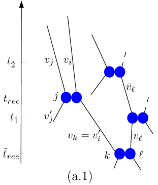
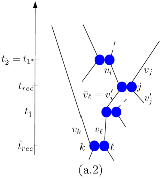
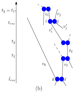
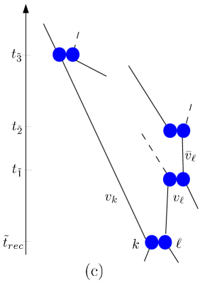
Figure 5. Case $t_{\tilde{1}}<t_{1^{*}}$, Degree of intertwinement between both recollisions

We therefore need to be more precise when describing the history of $(k,\ell)$. We denote by $(x_{k},x_{\ell})$ the positions of the pseudo-particles $k$ and $\ell$ at time $t_{\tilde{2}}$. We denote by $(v_{i},v_{j})$ (resp. $(v^{\prime}_{i},v^{\prime}_{j})$ ) the velocities of particles $i,j$ before the recollision (resp. after) the recollision $(i,j)$.

• We need a more precise geometric argument to ensure both that the first recollision occurs, and that it produces an outgoing velocity $v_{i}^{\prime}$ or $v_{j}^{\prime}$ in the ball $B(\bar{v}_{\ell},{\varepsilon}^{3/4})$. This is provided in Lemma B.1. Note that this case can be degenerate if $\tilde{2}=1^{*}$, which means that $\tilde{2}$ is also the parent of $\ell$.

• Again Lemma B.1 enables us to ensure both that the first recollision occurs, and that it produces an outgoing velocity $v_{i}^{\prime}$ or $v_{j}^{\prime}$ in the ball $B(v_{k},{\varepsilon}^{3/4})$. Note that this case can be degenerate if $\tilde{2}$ is also the parent of $k$.

• We know that $\tilde{2}>1^{*},2^{*}$. We then integrate over $dt_{\tilde{2}}dv_{\tilde{2}}d\nu_{\tilde{2}}$ the constraint of having small relative velocities $|v_{k}-\bar{v}_{\ell}|\leq{\varepsilon}^{3/4}$ and by (C.10) this gives a bound of the order of $O(R^{2}t{\varepsilon}^{3/4}|\log{\varepsilon}|)$. Then we apply Proposition 3.5 to recollision $(i,j)$ which involves parents $1^{*},2^{*}<\tilde{2}$. We are therefore in the situation (i).

• In that case combining (C.3) and (C.4), we deduce that

  $$\int{\bf 1}_{|v_{k}-\bar{v}_{\ell}|\leq{\varepsilon}^{\frac{3}{4}}}\displaystyle\prod_{m=\tilde{2},\tilde{3}}\,\big{|}\big{(}v_{m}-v_{a(m)}(t_{{m}}))\cdot\nu_{{m}}\big{)}\big{|}dt_{{m}}d\nu_{{m}}dv_{{m}}\leq CR^{5}t^{2}{\varepsilon}^{3/2}|\log{\varepsilon}|\,.$$

  For any fixed $\{\tilde{2},\tilde{3}\}$, this scenario will be labelled by $p=3$ hence

  $$\int{\bf 1}_{\mathcal{P}_{2}(a,3,\sigma)}\displaystyle\prod_{m\in\sigma}\,\big{|}\big{(}v_{m}-v_{a(m)}(t_{{m}}))\cdot\nu_{{m}}\big{)}\big{|}dt_{{m}}d\nu_{{m}}dv_{{m}}\leq CsR^{5}t^{2}{\varepsilon}^{3/2}|\log{\varepsilon}|\,.$$

Note the extra factor $s$, which appears for the same reasons as explained page 3.1.1.

6.2.2. Case 2: $t_{\tilde{1}}=t_{1^{*}}$

This is a very constrained case, as all the recolliding particles have the same first parent. We separate the analysis into two subcases.

2.1 Parallel recollisions. This case is depicted in Figure 6; the two recollisions take place with the same parent, but there is no direct link between the two couples of recolliding pseudo-particles $(i,j)$ and $(k,\ell)$, meaning as previously that the trajectory of $\ell$ and $k$ between time $t_{\tilde{1}}=t_{1^{*}}$ and $\tilde{t}_{rec}$ is unaffected by that of $i$ or $j$ on the same time interval.

Figure 6. $t_{\tilde{1}}=t_{1^{*}}$, parallel recollisions.

The analysis is postponed to Lemma B.2.

2.2 Recollisions in chain. In this case the two recollisions take place in chain (the trajectory of one of the recolliding particles $k$ or $\ell$ is affected by $i$ or $j$ between time $t_{\tilde{1}}=t_{1^{*}}$ and $\tilde{t}_{rec}$) (see Figure 7).

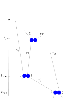
Figure 7. $t_{\tilde{1}}=t_{1^{*}}$, recollisions in chain.

This case is dealt with in Lemma B.3 and Lemma B.4 in Appendix B

6.2.3. Indexing with $\sigma$

So far the two recollisions have been described in terms of the recolliding particles $i,j,k,\ell$, however in Proposition 6.2 the sets $\mathcal{P}_{2}(a,p,\sigma)$ are not indexed by the recolliding particles but by the parents of these particles, i.e. by the degrees of freedom leading to these recollisions. Once the set $\sigma$ of parents is fixed, all the recolliding particles are not necessarily prescribed. Indeed for parallel recollisions or recollisions in chain, the set $\sigma$ could corresponds only to parents of $i$ in which case there is an extra combinatorial factor $s^{2}$ for choosing the other two recolliding particles $j,k$.

6.3. Estimate of $R_{N}^{K,>}$ (super exponential trees with multiple recollisions)

Proposition 6.1 comes from a careful summation of all elementary contributions. We therefore need the following refinement of Proposition 3.9.

Proposition 6.3.

We fix $z_{1}\in\mathbb{T}^{2}\times B_{R}$, a label $p\leq p_{0}$ and a set $\sigma\subset\{1,\dots,s\}$ of cardinal $|\sigma|\leq 5$. With the notation of Proposition 6.2, denoting $\eta=s^{2}t^{r}{\varepsilon}$, one has for $t\geq 1$

(6.4) $$\sum_{a\in\mathcal{A}_{s}}\int{\bf 1}_{\mathcal{T}_{2,s}}{\bf 1}_{\mathcal{P}_{2}(a,p,\sigma)}\,\Big{(}\prod_{i=2}^{s}\,\big{|}(v_{i}-v_{a(i)}(t_{i}))\cdot\nu_{i}\big{|}\Big{)} M_{\beta}^{\otimes s}\,dT_{2,s}d\Omega_{2,s}dV_{2,s}$$

$$\leq s^{5}(Ct)^{s-1}\eta M_{\beta/2}(v_{1})\,.$$

If we further specify that the last $n$ collision times have to be in an interval of length $h\leq 1$ (this constraint is denoted by $\mathcal{T}_{s-n+1,s}^{h}$) then

(6.5) $$\sum_{a\in\mathcal{A}_{s}}\int{\bf 1}_{\mathcal{T}_{2,s}}{\bf 1}_{\mathcal{T}_{s-n+1,s}^{h}}{\bf 1}_{\mathcal{P}_{2}(a,p,\sigma)}\;\Big{(}\prod_{i=2}^{s}\,\big{|}(v_{i}-v_{a(i)}(t_{i}))\cdot\nu_{i}\big{|}\Big{)}M_{\beta}^{\otimes s}\,dT_{2,s}d\Omega_{2,s}dV_{2,s}$$

$$\leq s^{5}(Ct)^{s-n-1}(Ch)^{n-5}\eta M_{\beta/2}(v_{1})\,.$$

Proof.

The proof of Proposition 6.3 follows the same lines as the one of Proposition 3.9. The additional difficulty is to control the divergence in $R^{r}$ in the estimate (6.1) on the recollisions. To do so, we decompose the total energy into blocks

$$\sum_{a\in\mathcal{A}_{s}}\int{\bf 1}_{\mathcal{T}_{2,s}}{\bf 1}_{\mathcal{P}_{2}(a,p,\sigma)}\left(\prod_{i=2}^{s}\,\big{|}(v_{a(i)}(t_{i})-v_{i})\cdot\nu_{i}\big{|}\right)M_{\beta}^{\otimes s}dT_{2,s}d\Omega_{2,s}dV_{2,s}$$

$$\qquad\qquad\leq\sum_{m=1}^{C|\log|\log{\varepsilon}||}\sum_{a\in\mathcal{A}_{s}}\int{\bf 1}_{\mathcal{T}_{2,s}}{\bf 1}_{\mathcal{P}_{2}(a,p,\sigma)}{\bf 1}_{\{2^{m-1}\leq|V_{s}|\leq 2^{m}\}}$$

$$\qquad\qquad\qquad\qquad\qquad\qquad\times\left(\prod_{i=2}^{s}\,\big{|}(v_{a(i)}(t_{i})-v_{i})\cdot\nu_{i}\big{|}\right)M_{\beta}^{\otimes s}dT_{2,s}d\Omega_{2,s}dV_{2,s}\,.$$

Situations $(i)$ and $(ii)$ in Proposition 6.2 will be dealt with separately. We start with $\mathcal{P}_{2}(a,p,\sigma)$ for $p>2$ which depends only on the configurations at time $t_{\sigma_{-}}$ and on the parameters labelled by $\sigma$. Using Proposition 2.5, the contribution of the trees after $\sigma_{-}$ (without the labels in $\sigma$) is estimated as in (3.17)

(6.6) $$\sum_{(a(j))_{j>\sigma_{-}}}\left(\prod_{i>\sigma_{-},\atop i\not\in\sigma}\,\big{|}(v_{i}-v_{a(i)}(t_{i}))\cdot\nu_{i}\big{|}\right)M_{5\beta/6}^{\otimes s}(V_{s})\leq(Cs)^{s-\sigma_{-}-3}M_{2\beta/3}^{\otimes\sigma_{-}}(V_{\sigma_{-}})\,.$$

Then for any $R=2^{m}$, we integrate with respect to the $|\sigma|$ variables indexed by $\sigma$ and get

(6.7) $$\int{\bf 1}_{\mathcal{P}_{2}(a,p,\sigma)}{\bf 1}_{|\hat{V}|\leq R}\,\prod_{i\in\sigma}\,\big{|}(v_{a(i)}(t_{i})-v_{i})\cdot\nu_{i}\big{|}\,dT_{\sigma}d\Omega_{\sigma}dV_{\sigma}\leq\eta\,R^{r},$$

with $\hat{V}=\{v_{i}\quad i\leq\sigma_{-}\ \text{and}\ i\in\sigma\}$. The main difference with the proof of Proposition 3.9 is that we use once again the Maxwellian tails to get

(6.8) $$\sup_{V_{s}}\Big{\{}{\bf 1}_{\{R/2\leq|V_{s}|\leq R\}}R^{r}\,M_{\beta/6}^{\otimes s}(V_{s})\Big{\}}\leq C^{s}\exp(-CR^{2})\,,$$

for some constant $C$ depending only on $r$ and $\beta$. This controls the divergence in $R$ arising in (6.7). An additional factor $s^{|\sigma|}$ takes into account the choices $a(i)$ for the labels $i$ belonging to $\sigma$. Finally the contribution of the collision trees before $\sigma_{-}$ can be estimated by Proposition 2.5 loosing an additional $\beta/6$ in the exponential weight.

The contribution of the sets $\mathcal{P}_{2}(a,p,\sigma)$ for $p\leq 2$ can be estimated with minor changes in the order of integration in order to decouple the contraints on both recollisions. First the combinatorics of the trees after $\sigma_{+}$ is estimated, then the geometric constraint at $\sigma_{+}$ is evaluated. Then the combinatorics of the trees up to $\max(\sigma\setminus\{\sigma_{+}\})$, and the (independent) constraints to be $\mathcal{P}_{1}(a,p,\sigma\setminus\{\sigma_{+}\})$ . Finally it remains to take into account the contribution of the rest of the labels. The large velocities are bounded also as in (6.8).

The final step is to integrate with respect to the remaining time variables. We only retain the condition for the times $(t_{i})_{i\notin\sigma}$.

• In the first case, we get a simplex of dimension $s-1-|\sigma|$, the volume of which is

  $${t^{s-1-|\sigma|}\over(s-1-|\sigma|)!}\leq C^{s}{t^{s-1-|\sigma|}\over s^{s-1-|\sigma|}}\,,$$

  by Stirling’s formula.

• In the second case, we have to add the condition that the last $n$ times have to be in an interval of length $h\leq 1$. The worst situation is when all times $(t_{i})_{i\in\sigma}$ are in this small time interval, as we loose the corresponding smallness. More precisely, we get

  $${t^{s-1-n}\over(s-1-n)!}{h^{n-|\sigma|}\over(n-|\sigma|)!}\leq C^{s}{t^{s-1-n}h^{n-|\sigma|}\over s^{s-1-|\sigma|}}\,\cdotp$$

We thus conclude that for any $R$,

$$\sum_{a\in\mathcal{A}_{s}}\int{\bf 1}_{\mathcal{T}_{2,s}}{\bf 1}_{\mathcal{P}_{2}(a,p,\sigma)}{\bf 1}_{\{R/2\leq|V_{s}|\leq R\}}\left(\prod_{i=2}^{s}\,\big{|}(v_{a(i)}(t_{i})-v_{i})\cdot\nu_{i}\big{|}\right)M_{\beta}^{\otimes s}dT_{2,s}d\Omega_{2,s}dV_{2,s}$$

$$\leq s^{4}(Ct)^{s-1}\eta e^{-CR^{2}}M_{\frac{\beta}{2}}(v_{1})\,,$$

and

$$\sum_{a\in\mathcal{A}_{s}}\int{\bf 1}_{\mathcal{T}_{2,s}} {\bf 1}_{\mathcal{T}_{s-n+1,s}^{h}}{\bf 1}_{\mathcal{P}_{2}(a,p,\sigma)}{\bf 1}_{\{R/2\leq|V_{s}|\leq R\}}$$

$$\qquad\times\left(\prod_{i=2}^{s}\,\big{|}(v_{a(i)}(t_{i})-v_{i})\cdot\nu_{i}\big{|}\right)M_{\beta}^{\otimes s}dT_{2,s}d\Omega_{2,s}dV_{2,s}$$

$$\qquad\qquad\leq s^{|\sigma|}(Ct)^{s-n-1}(Ch)^{n-|\sigma|}\eta e^{-CR^{2}}M_{\frac{\beta}{2}}(v_{1})\,,$$

where all constants are independent of $R$. The factor $s^{|\sigma|}$ comes from the summation over the possible choices of $(a(i))_{i\in\sigma}$. Finally, the result follows by summing over $R=2^{m}$.

∎

Proof of Proposition 6.1.

The occurrence of multiple recollisions in a collision tree of size $s$ can be estimated by summing over all the possible $\sigma$ and using Proposition 6.3

$$\sum_{\sigma}\sum_{a\in\mathcal{A}_{s}}\int{\bf 1}_{\mathcal{T}_{2,s}}{\bf 1}_{\mathcal{T}_{s-n+1,s}^{h}}{\bf 1}_{\mathcal{P}_{2}(a,p,\sigma)}\left(\prod_{i=2}^{s}\,\big{|}(v_{a(i)}(t_{i})-v_{i})\cdot\nu_{i}\big{|}\right){{\bf 1}_{{\mathcal{V}}_{s}}}f_{N}^{(s)}(t-kh)dT_{2,s}d\Omega_{2,s}dV_{2,s}$$

$$\leq N\exp(C\alpha^{2})s^{12}(Ct)^{s-n-1}(Ch)^{n-5}\,t^{r}{\varepsilon}\,M_{\frac{\beta}{2}}(v_{1})\,,$$

where the a priori $L^{\infty}$-bound (2.13) has been used. The factor $s^{12}$ comes from the contribution $s^{2}$ in the definition of $\eta$, $s^{5}$ in Proposition 6.3, and from the fact that there are at most $O(s^{5})$ choices for the elements of $\sigma$.

Choosing $n_{k}=2^{k}n_{0}$, we then have, since $\alpha^{2}th\ll 1$,

$$\Big{|}R_{N}^{K,>}(t,z_{1})\Big{|} \leq M_{\frac{\beta}{2}}(v_{1})N{{\varepsilon}t^{r}\over h^{5}}\exp(C\alpha^{2})\sum_{k=1}^{K}\sum_{j_{1}=0}^{n_{1}-1}\!\!\dots\!\!\sum_{j_{k-1}=0}^{n_{k-1}-1}\sum_{j_{k}=n_{k}}^{N-J_{k-1}}(C\alpha t)^{J_{k-1}}(C\alpha h)^{j_{k}}J_{k}^{12}$$

$$\leq M_{\frac{\beta}{2}}(v_{1})\exp(C\alpha^{2}){t^{r}\over h^{5}}\sum_{k=1}^{K}\sum_{j_{1}=0}^{n_{1}-1}\!\!\dots\!\!\sum_{j_{k-1}=0}^{n_{k-1}-1}n_{k}^{12}(C\alpha h)^{n_{k}}(C\alpha t)^{J_{k-1}}$$

$$\leq M_{\frac{\beta}{2}}(v_{1})\exp(C\alpha^{2}){t^{r}\over h^{5}}\sum_{k=1}^{K}2^{k^{2}}\left(C\alpha^{2}ht\right)^{2^{k}n_{0}}$$

$$\leq M_{\frac{\beta}{2}}(v_{1})\exp(C\alpha^{2}){t^{r}\over h^{5}}(C\alpha^{2}ht)^{n_{0}}\,,$$

and Proposition 6.1 follows with $h\leq{\gamma}/{\exp(C\alpha^{2})T^{3}}$ as soon as $n_{0}$ is large enough. Note that this is the only argument in which $n_{0}$ needs to be tuned. ∎

7. Truncation of large velocities

In this section, we prove that collision trees with large velocities contribute very little to the iterated Duhamel series. As a consequence, the error term $R_{N}^{K,vel}$ introduced in (2.28) vanishes. This holds also for the analogous term in the Boltzmann hierarchy

$$\bar{R}^{K,vel}(t):=\sum_{j_{1}=0}^{n_{1}-1}\!\!\dots\!\!\sum_{j_{K}=0}^{n_{K}-1}\bar{Q}_{1,J_{1}}(h)\,\bar{Q}_{J_{1},J_{2}}(h)\dots\bar{Q}_{J_{K-1},J_{K}}(h)\,\left(f^{(J_{K})}_{0}{\bf 1}_{|V_{J_{K}}|^{2}>C_{0}|\log{\varepsilon}|}\right)$$

$$+\sum_{k=1}^{K}\;\sum_{j_{1}=0}^{n_{1}-1}\!\!\dots\!\!\sum_{j_{k-1}=0}^{n_{k-1}-1}\sum_{j_{k}\geq n_{k}}\;\bar{Q}_{1,J_{1}}(h)\dots\bar{Q}_{J_{k-1},J_{k}}(h)\left(f^{(J_{k})}(t-kh){\bf 1}_{|V_{J_{k}}|^{2}>C_{0}|\log{\varepsilon}|}\right).$$

The contribution of the large energies can be estimated by the following result.

Proposition 7.1.

There exists a constant $C_{0}\geq 0$ such that for all $t\in[0,T]$ and $\alpha^{2}hT\ll 1$

$$\left|R_{N}^{K,vel}(t)\right|+\left|\bar{R}^{K,vel}(t)\right|\leq\exp(C\alpha^{2})n_{0}^{K}2^{K^{2}}Ê(C\alpha T)^{n_{0}\cdot 2^{K}}{\varepsilon}M_{\beta/2}(z_{1}),$$

with the sequence $n_{k}=2^{k}n_{0}$.

Proof.

The remainders $R_{N}^{K,vel}$ (2.28) and $\bar{R}^{K,vel}$ are made of two contributions, the first one is an energy cut-off for the Duhamel series up to time 0 (with a number of collisions less than $2^{K}n_{0}$) and the second one is a truncation at an intermediate time corresponding to a large number of collisions. We shall consider only the BBGKY hierarchy as $\bar{R}^{K,vel}$ can be treated similarly.

For the Duhamel series up to time 0, we notice that for $C_{0}$ large enough

$$\left|f^{(J_{k})}_{N}(0){\bf 1}_{|V_{J_{k}}|^{2}\geq C_{0}|\log{\varepsilon}|}\right| \leq C^{J_{k}}NM^{\otimes J_{k}}_{\beta}{\bf 1}_{|V_{J_{k}}|^{2}\geq C_{0}|\log{\varepsilon}|}\;\|g_{\alpha,0}\|_{L^{\infty}(\mathbb{D})}$$

$$\leq\exp(C\alpha^{2})C^{J_{k}}NM_{5\beta/6}^{\otimes J_{k}}\exp\left(-\frac{\beta}{12}|V_{J_{k}}|^{2}\right){\bf 1}_{|V_{J_{k}}|^{2}\geq C_{0}|\log{\varepsilon}|}$$

$$\leq{\varepsilon}\exp(C\alpha^{2})C^{J_{k}}M_{5\beta/6}^{\otimes J_{k}}\,.$$

Then using the fact that

$$\big{|}Q_{1,J_{1}}(h)Q_{J_{1},J_{2}}(h)\dots Q_{J_{k-1},J_{k}}(h)\big{|}\leq|Q_{1,J_{k-1}}|(t)\,|Q_{J_{k-1},J_{k}}|(h)\,,$$

together with Proposition 2.5, we get

$$\sum_{k=1}^{K}\sum_{j_{i}<n_{i}} \left|Q_{1,J_{1}}(h)Q_{J_{1},J_{2}}(h)\dots Q_{J_{k-1},J_{k}}(h)\,\big{(}f^{(J_{k})}_{N}(0){\bf 1}_{|V_{J_{k}}|^{2}\geq C_{0}|\log{\varepsilon}|}\big{)}\right|$$

$$\leq\exp(C\alpha^{2})\sum_{k=1}^{K}\sum_{j_{i}<n_{i}}(C\alpha t)^{J_{K}}{\varepsilon}M_{\beta/2}(z_{1})$$

$$\leq\exp(C\alpha^{2})n_{0}^{K}2^{K^{2}}\,(C\alpha T)^{2^{K+1}n_{0}}{\varepsilon}M_{\beta/2}(z_{1})\,.$$

From the maximum principle (2.15), we further deduce that for $C_{0}$ large enough

$$\big{|}f_{N}^{(J_{k})}(t-kh){\bf 1}_{|V_{J_{k}}|^{2}\geq C_{0}|\log{\varepsilon}|}\big{|}\leq{\varepsilon}\exp(C\alpha^{2})C^{J_{k}}M_{5\beta/6}^{\otimes J_{k}},$$

so

$$\sum_{j_{k}\geq n_{k}} \left|Q_{1,J_{1}}(h)Q_{J_{1},J_{2}}(h)\dots Q_{J_{k-1},J_{k}}(h)\,\big{(}f^{(J_{k})}_{N}(t-kh){\bf 1}_{|V_{J_{k}}|^{2}\geq C_{0}|\log{\varepsilon}|}\big{)}\right|$$

$$\qquad\qquad\qquad\qquad\qquad\qquad\leq\exp(C\alpha^{2})(C\alpha t)^{J_{k-1}}(C\alpha h)^{n_{k}}{\varepsilon}M_{\beta/2}(z_{1})\,,$$

as soon as $\alpha h\ll 1$.

Recalling (3.19), since $\alpha^{2}th\ll 1$, we can sum the different contributions corresponding to a large number of collisions

$$\sum_{k=1}^{K}\sum_{j_{i}<n_{i}\atop i\leq k-1} \sum_{j_{k}\geq n_{k}}\left|Q_{1,J_{1}}(h)Q_{J_{1},J_{2}}(h)\dots Q_{J_{k-1},J_{k}}(h)\,\big{(}f^{(J_{k})}_{N}(t-kh){\bf 1}_{|V_{J_{k}}|^{2}\geq C_{0}|\log{\varepsilon}|}\big{)}\right|$$

$$\leq\exp(C\alpha^{2})\sum_{k=1}^{K}\sum_{j_{i}<n_{i}\atop i\leq k-1}(C\alpha t)^{J_{k-1}}(C\alpha h)^{n_{k}}{\varepsilon}M_{\beta/2}(z_{1})$$

$$\leq\exp(C\alpha^{2})\,\,{\varepsilon}\sum_{k=1}^{K}n_{0}^{k}2^{k^{2}}(C\alpha^{2}th)^{n_{0}\,2^{k}}M_{\beta/2}(z_{1})$$

$$\leq\exp(C\alpha^{2})\,{\varepsilon}M_{\beta/2}(z_{1})\,.$$

Combining both estimates concludes the proof of Proposition 7.1. ∎

8. End of the proof of Theorem 1.2, and open problems

8.1. Proof of Theorem 1.2

In this section, we gather all the error estimates obtained in the previous section and conclude the proof of Theorem 1.2. Fix $T>1$ and $t\in[0,T]$.

We recall that due to (2.23) and (2.24) we have

$$f_{N}^{(1)}(t)=f^{(1,K)}_{N}(t)+R_{N}^{K}(t)$$

and

$$R_{N}^{K}(t)=R_{N}^{K,0}(t)+R_{N}^{K,1}(t)+R_{N}^{K,>}(t)+R_{N}^{K,vel}(t)\,.$$

Similarly

$$f^{(1)}(t)=\bar{f}^{(1,K)}(t)+\bar{R}^{K}(t)+\bar{R}^{K,vel}(t)\,.$$

From Proposition 3.1, we know that the difference between the dominant parts is

$$\Big{\|}f^{(1,K)}_{N}(t)-\bar{f}^{(1,K)}(t)\Big{\|}_{L^{2}}\leq(C\alpha T)^{2^{K+1}n_{0}}\exp(C\alpha^{2})\Big{(}{\varepsilon}|\log{\varepsilon}|^{10}+{{\varepsilon}\over\alpha}\Big{)}\,.$$

This contribution will be small provided that the number of collisions is bounded by

(8.1) $$K={T\over h}\ll\log|\log{\varepsilon}|,\qquad\alpha\ll\sqrt{\log|\log{\varepsilon}|}\,.$$

Let us now gather the estimates for the remainders, under the assumption that

(8.2) $$h\leq\frac{\gamma^{2}}{\exp(C\alpha^{2})T^{3}},$$

for some $C$ large enough.

By Propositions 4.1 and 4.8, we have

$$\Big{\|}R_{N}^{K,0}(t)\Big{\|}_{L^{2}}\leq\gamma\quad\text{and}\quad\Big{\|}\bar{R}^{K}(t)\Big{\|}_{L^{2}(\mathbb{D})}\leq\gamma\,.$$

By Proposition 5.1, the remainder for 1 recollision is bounded by

$$\Big{\|}R_{N}^{K,1}(t)\Big{\|}_{L^{2}}\leq{\varepsilon}^{1/2}|\log{\varepsilon}|^{6}{\gamma\over h}.$$

From Proposition 6.1, the remainder for multiple recollisions is bounded by

$$\Big{\|}R_{N}^{K,>}(t)\Big{\|}_{L^{2}}\leq\gamma\,.$$

By Proposition 7.1 the remainders for large velocities satisfy, as soon as $\alpha h\ll 1$,

$$\Big{\|}R_{N}^{K,vel}(t)\Big{\|}_{L^{2}}+\Big{\|}\bar{R}^{K,vel}(t)\Big{\|}_{L^{2}}\leq\exp(C\alpha^{2})n_{0}^{K}2^{K^{2}}(C\alpha T)^{2^{K+1}n_{0}}{\varepsilon}\,,$$

which is small under (8.1), (8.2).

The convergence estimate (1.21) is then obtained by combining conditions (8.1) and (8.2)

$$\Big{\|}f_{N}^{(1)}(t)-f^{(1)}(t)\Big{\|}_{L^{2}} \leq\Big{\|}f^{(1,K)}_{N}(t)-\bar{f}^{(1,K)}(t)\Big{\|}_{L^{2}}+\Big{\|}R_{N}^{K,0}(t)\Big{\|}_{L^{2}}+\Big{\|}\bar{R}^{K}(t)\Big{\|}_{L^{2}}$$

$$\qquad\qquad+\Big{\|}R_{N}^{K,1}(t)\Big{\|}_{L^{2}}+\Big{\|}R_{N}^{K,>}(t)\Big{\|}_{L^{2}}+\Big{\|}R_{N}^{K,vel}(t)\Big{\|}_{L^{2}}+\Big{\|}\bar{R}^{K,vel}(t)\Big{\|}_{L^{2}}$$

$$\leq\frac{\exp(C\alpha^{2})T^{2}}{\sqrt{\log|\log{\varepsilon}|}}\,\cdotp$$

This concludes the proof of Theorem 1.2. ∎

8.2. Open problems

In this final section, we collect some open problems related to those treated in this paper.

Finite range potentials.

We expect the same convergence results to hold if microscopic interactions are described by a repulsive compactly supported potential (instead of the singular hard-sphere interactions). The proof then involves truncated marginals and cluster estimates as in [9, 22]. With the present scaling, there is however a difficulty to control triple interactions, the size of which is critical (see the computations of Appendix B). Note that the case of a potential, non compactly supported, is rigorously analyzed for the first time in [2] in the linear case.

Higher dimensions.

We also expect the convergence results to extend to higher dimensions and it has been proven for short times in [4]. However, there are two important simplifications in dimension 2. The first one is due to the fact that the inverse partition function associated with the exclusion is bounded uniformly in $N$, as shown in (2.17); in particular this makes it possible to propagate somehow the initial form of the initial datum and to decompose the marginals of the solution in a quasi-orthogonal form; see Section 4. The second one is related to the control of recollisions: we have seen in this paper (namely in Section 6) that the probability of having pseudo-dynamics with multiple recollisions is $O({\varepsilon})$, which balances exactly the $O(N)$ size of the $L^{\infty}$ norm of the solution, and that is not the case in higher dimension in the Boltzmann-Grad scaling since ${\varepsilon}\sim N^{\frac{1}{1-d}}$.

Spatial Domain.

The spatial domain we consider here is the torus $\mathbb{T}^{2}$, which is equivalent to a rectangular box with specular reflection on the boundary. To extend the analysis to more general domains, we would need a geometric property of the free flow on these domains, stating roughly that the probability, in velocities, for two trajectories to approach at a distance ${\varepsilon}$ on a fixed time interval $[0,T]$ is vanishing in the limit ${\varepsilon}\to 0$.

Dissipation.

The control on the higher order cumulants $g_{N}^{m}$ is the key to improve the convergence time with respect to Lanford’s original argument. This estimate can be seen as playing the role of the dissipation on the limiting equation. We indeed have

$$\frac{1}{N}\int{f_{N}^{2}(t)\over M^{\otimes N}_{\beta}}dZ_{N}=\|g_{N}^{1}(t)\|^{2}_{L^{2}_{\beta}(\mathbb{D})}+\sum_{m=2}^{N}{\binom{N}{m}\over N}\|g_{N}^{m}(t)\|^{2}_{L^{2}_{\beta}(\mathbb{D}^{m})}=\frac{1}{N}\int{f_{N,0}^{2}\over M^{\otimes N}_{\beta}}dZ_{N}\,.$$

to be compared to

$$\|g(t)\|^{2}_{L^{2}_{\beta}(\mathbb{D})}+\alpha\int_{0}^{t}\int M_{\beta}g\mathcal{L}_{\beta}g(s,x,v)dvdxds=\|g_{0}\|^{2}_{L^{2}_{\beta}(\mathbb{D})}$$

for the limiting equation.

Stochastic corrections.

In [28], Spohn studied the stochastic fluctuations around the Boltzmann equation and computed the variance of the fluctuation field in a non-equilibrium state

$$\zeta^{N}(g,t)=\frac{1}{\sqrt{N}}\left(\chi^{N}(g,t)-\langle\chi^{N}(g,t)\rangle\right)\quad\text{with}\quad\chi^{N}(g,t)=\sum_{i=1}^{N}g(z_{i}(t))\,,$$

where $g$ is a smooth function and $\langle\cdot\rangle$ stands for the mean. It would be of great interest to prove that the limiting field is Gaussian and to derive, even for short times, the fluctuating hydrodynamics.

Appendix A The linearized Boltzmann equation and its fluid limits

For the sake of completeness, we recall here some by now classical results about the linearized Boltzmann equation (1.14)

(A.1) $${1\over\alpha^{q}}{\partial}_{t}g_{\alpha}+v\cdot\nabla_{x}g_{\alpha}=-\alpha\mathcal{L}_{\beta}g_{\alpha}$$

$$\mathcal{L}_{\beta}g(v)=\int M_{\beta}(v_{1})\Big{(}g(v)+g(v_{1})-g(v^{\prime})-g(v_{1}^{\prime})\Big{)}\big{(}(v_{1}-v)\cdot\nu\big{)}_{+}d\nu dv_{1}$$

and its hydrodynamic limits as $\alpha\to\infty$ (for $q=0,1$). The results below are valid in any dimension $d\geq 2$, thus contrary to the rest of this article, we assume the space dimension to be $d$.

Because of the scaling invariance of the collision kernel, we shall actually restrict our attention in the sequel to the case where $M_{\beta}$ is the reduced centered Gaussian, i.e. $\beta=1$ (and we omit the subscript $\beta$ in the following). The collision operator (A.1) will be denoted by $\mathcal{L}$.

A.1. The functional setting

The linearized Boltzmann operator $\mathcal{L}$ has been studied extensively (since it governs small solutions of the nonlinear Boltzmann equation). In the case of non singular cross sections, its spectral structure was described by Grad [12]. The main result is that it satisfies the Fredholm alternative in a weighted $L^{2}$ space. In the following we define the collision frequency

$$a(|v|):=\int M(v_{1})\big{(}(v_{1}-v)\cdot\nu\big{)}_{+}d\nu dv_{1}$$

which satisfies, for some $C>1$,

$$0<a_{-}\leq a(|v|)\leq C(1+|v|)\,.$$

Proposition A.1.

The linear collision operator $\mathcal{L}$ defined by (A.1) is a nonnegative unbounded self-adjoint operator on $L^{2}(Mdv)$ with domain

$$\mathcal{D}(\mathcal{L})=\{g\in L^{2}(Mdv)\,|\,ag\in L^{2}(Mdv)\}=L^{2}(\mathbb{R}^{d};aM(v)dv)$$

and nullspace

$$\operatorname{Ker}(\mathcal{L})=\operatorname{span}\{1,v_{1},\dots,v_{d},|v|^{2}\}\,.$$

Moreover the following coercivity estimate holds: there exists $C>0$ such that, for each $g$ in $\mathcal{D}(\mathcal{L})\cap(\operatorname{Ker}(\mathcal{L}))^{\perp}$

$$\int g\mathcal{L}g(v)M(v)dv\geq C\|g\|_{L^{2}(aMdv)}^{2}\,.$$

Sketch of proof.

$\bullet$ The first step consists in characterizing the nullspace of $\mathcal{L}$. It must contain the collision invariants since the integrand in $\mathcal{L}g$ vanishes identically if $g(v)=1,v_{1},v_{2},\dots,v_{d}$ or $|v|^{2}$. Conversely, from the identity,

$$\int\psi\mathcal{L}gMdv=\frac{1}{4}\int(\psi\!+\!\psi_{1}\!-\!\psi^{\prime}\!-\!\psi^{\prime}_{1})(g\!+\!g_{1}\!-\!g^{\prime}\!-\!g^{\prime}_{1})\big{(}(v_{1}-v)\cdot\nu\big{)}_{+}Mdvdv_{1}d\nu\,,$$

where we have used the classical notation

$$g_{1}:=g(v_{1})\,,\quad g^{\prime}=g(v^{\prime})\ ,\quad g^{\prime}_{1}=g(v^{\prime}_{1})\,,$$

we deduce that, if $g$ belongs to the nullspace of $\mathcal{L}$, then

$$g+g_{1}=g^{\prime}+g^{\prime}_{1}\,,$$

which entails that $g$ is a linear combination of $1,v_{1}$, $v_{2},\dots,v_{d}$ and $|v|^{2}$ (see for instance [21]).

Note that the same identity shows that $\mathcal{L}$ is self-adjoint.

$\bullet$ In order to establish the coercivity of the linearized collision operator $\mathcal{L}$, the key step is then to introduce Hilbert’s decomposition [16], showing that $\mathcal{L}$ is a compact perturbation of a multiplication operator :

$$\mathcal{L}g(v)=a(|v|)g(v)-\mathcal{K}g(v)\,.$$

Proving that $\mathcal{K}$ is a compact integral operator on $L^{2}(Mdv)$ relies on intricate computations using Carleman’s parametrization of collisions (which we also use in this paper for the study of recollisions). We shall not perform them here (see [16]).

Because $a$ is bounded from below, $\mathcal{L}$ has a spectral gap, which provides the coercivity estimate. ∎

Proposition A.1, along with classical results on maximal accretive operators, imply the following statement.

Proposition A.2.

Let $g_{0}\in L^{2}(Mdvdx)$. Then, for any fixed $\alpha$, there exists a unique solution $g_{\alpha}\in C(\mathbb{R}^{+},L^{2}(Mdvdx))\cap C^{1}(\mathbb{R}^{+}_{*},L^{2}(Mdvdx))\cap C(\mathbb{R}^{+}_{*},L^{2}(Madvdx))$ to the linearized Boltzmann equation (A.1). It satisfies the scaled energy inequality

(A.2) $$\|g_{\alpha}(t)\|^{2}_{L^{2}(Mdvdx)}+\alpha^{1+q}\int_{0}^{t}\int g_{\alpha}\mathcal{L}g_{\alpha}(t^{\prime})Mdvdxdt^{\prime}\leq\|g_{0}\|_{L^{2}(Mdv)}^{2}\,.$$

A.2. The acoustic and Stokes limit

The starting point for the study of hydrodynamic limits is the energy inequality (A.2). The uniform $L^{2}$ bound on $(g_{\alpha})$ implies that, up to extraction of a subsequence,

(A.3) $$g_{\alpha}\rightharpoonup g\hbox{ weakly in }L^{2}_{loc}(dt,L^{2}(Mdvdx))\,.$$

Let $\Pi$ be the orthogonal projection on the kernel of $\mathcal{L}$. The dissipation, together with the coercivity estimate in Proposition A.1, further provides

$$\|g_{\alpha}-\Pi g_{\alpha}\|_{L^{2}(Madvdxdt)}=O(\alpha^{-(q+1)/2})\,,$$

from which we deduce that

(A.4) $$g(t,x,v)=\Pi g(t,x,v)\equiv\rho(t,x)+u(t,x)\cdot v+\theta(t,x){|v|^{2}-d\over 2}\,\cdotp$$

If the Mach number $\alpha^{q}$ is of order 1, i.e. for $q=0$, one obtains asymptotically the acoustic equations. Denoting by $\langle\cdot\rangle$ the average with respect to the measure $Mdv$, we indeed have the following conservation laws

$${\partial}_{t}\langle g_{\alpha}\rangle+\nabla_{x}\cdot\langle g_{\alpha}v\rangle=0\,,$$

$${\partial}_{t}\langle g_{\alpha}v\rangle+\nabla_{x}\cdot\langle g_{\alpha}v\otimes v\rangle=0\,,$$

$${\partial}_{t}\langle g_{\alpha}|v|^{2}\rangle+\nabla_{x}\cdot\langle g_{\alpha}v|v|^{2}\rangle=0\,.$$

From (A.3) and (A.4) we then deduce that $(\rho,u,\theta)$ satisfy

(A.5) $${\partial}_{t}\rho+\nabla_{x}\cdot u=0\,,$$

$${\partial}_{t}u+\nabla_{x}(\rho+\theta)=0\,,$$

$${\partial}_{t}\theta+\frac{2}{d}\nabla_{x}\cdot u=0\,.$$

By uniqueness of the limiting point, we get the convergence of the whole family $(g_{\alpha})_{\alpha>0}$.

Since the limiting distribution $g$ satisfies the energy equality

$$\|g\|^{2}_{L^{2}(Mdvdx)}=\|g_{0}\|_{L^{2}(Mdvdx)}^{2}$$

or equivalently

$$\|g\|^{2}_{L^{2}(Mdvdx)}+\alpha\int_{0}^{t}\int g\mathcal{L}gMdvdx=\|\Pi g_{0}\|_{L^{2}(Mdvdx)}^{2}\,,$$

convergence is strong as soon as $g_{0}=\Pi g_{0}$. We thus have the following result (see [10] and references therein).

Proposition A.3.

Let $g_{0}\in L^{2}(Mdvdx)$. For all $\alpha$, let $g_{\alpha}$ be a solution to the scaled linearized Boltzmann equation (A.1) with $q=0$. Then, as $\alpha\to\infty$, $g_{\alpha}$ converges weakly in $L^{2}_{loc}(dt,L^{2}(Mdvdx))$ to the infinitesimal Maxwellian $\displaystyle g=\rho+u\cdot v+\frac{1}{2}\theta(|v|^{2}-d)$ where $(\rho,u,\theta)$ is the solution of the acoustic equations (A.5) with initial datum $\displaystyle(\langle g_{0}\rangle,\langle g_{0}v\rangle,\langle g_{0}\frac{1}{d}(|v|^{2}-d)\rangle)$.

The convergence holds strongly in $L^{\infty}_{t}(L^{2}(Mdvdx))$ provided that $g_{0}=\Pi g_{0}$.

In the diffusive regime, i.e. for $q=1$, the moment equations state

$${1\over\alpha}{\partial}_{t}\langle g_{\alpha}\rangle+\nabla_{x}\cdot\langle g_{\alpha}v\rangle=0\,,$$

$${1\over\alpha}{\partial}_{t}\langle g_{\alpha}v\rangle+\nabla_{x}\cdot\langle g_{\alpha}v\otimes v\rangle=0\,,$$

$${1\over\alpha}{\partial}_{t}\langle g_{\alpha}|v|^{2}\rangle+\nabla_{x}\cdot\langle g_{\alpha}v|v|^{2}\rangle=0\,.$$

From (A.3) and (A.4) we deduce that

$$\nabla_{x}\cdot u=0\,,\quad\nabla_{x}(\rho+\theta)=0\,,$$

referred to as incompressibility and Boussinesq constraints.

To characterize the mean motion, we then have to filter acoustic waves, i.e. to project on the kernel of the acoustic operator

$${\partial}_{t}P\langle g_{\alpha}v\rangle+\alpha P\nabla_{x}\cdot\langle g_{\alpha}(v\otimes v-\frac{1}{2}|v|^{2}Id)\rangle=0\,,$$

$${\partial}_{t}\langle g_{\alpha}({|v|^{2}\over d+2}-1)\rangle+\alpha\nabla_{x}\cdot\langle g_{\alpha}v({|v|^{2}\over d+2}-1)\rangle=0\,,$$

where $P$ is the Leray projection on divergence free vector fields. Define the kinetic momentum flux $\displaystyle\Phi(v)=v\otimes v-\frac{1}{d}|v|^{2}Id$ and the kinetic energy flux $\displaystyle\Psi(v)=\frac{1}{d+2}v(|v|^{2}-d-2)$. As $\Phi,\Psi$ belong to $(\operatorname{Ker}\mathcal{L})^{\perp}$, and $\mathcal{L}$ is a Fredholm operator, there exist pseudo-inverses $\tilde{\Phi},\tilde{\Psi}\in(\operatorname{Ker}\mathcal{L})^{\perp}$ such that $\Phi=\mathcal{L}\tilde{\Phi}$ and $\Psi=\mathcal{L}\tilde{\Psi}$. Then,

$${\partial}_{t}P\langle g_{\alpha}v\rangle+\alpha P\nabla_{x}\cdot\langle\mathcal{L}g_{\alpha}\tilde{\Phi}\rangle=0\,,$$

$${\partial}_{t}\langle g_{\alpha}({|v|^{2}\over d+2}-1)\rangle+\alpha\nabla_{x}\cdot\langle\mathcal{L}g_{\alpha}\tilde{\Psi}\rangle=0\,.$$

Using the equation

$$\alpha\mathcal{L}g_{\alpha}=-v\cdot\nabla_{x}g_{\alpha}-\frac{1}{\alpha}{\partial}_{t}g_{\alpha}$$

the Ansatz (A.4), and taking limits in the sense of distributions, we get

(A.6) $$\nabla_{x}\cdot u=0,\quad\nabla_{x}(\rho+\theta)=0\,,$$

$${\partial}_{t}u-\mu\Delta_{x}u=0\,,$$

$${\partial}_{t}\theta-\kappa\Delta_{x}\theta=0\,.$$

These are exactly the Stokes-Fourier equations with

$$\mu=\frac{1}{(d-1)(d+2)}\langle\Phi:\tilde{\Phi}\rangle\quad\text{and}\quad\kappa=\frac{2}{d(d+2)}\langle\Psi\cdot\tilde{\Psi}\rangle.$$

As previously, the limit is unique and the convergence is strong provided that the initial datum is well-prepared, i.e. if

(A.7) $$g_{0}(x,v)=u_{0}\cdot v+\frac{1}{2}\theta_{0}(|v|^{2}-(d+2))\hbox{ with }\nabla_{x}\cdot u_{0}=0\,.$$

One can therefore prove the following result.

Proposition A.4.

Let $g_{0}\in L^{2}(Mdvdx)$. For all $\alpha$, let $g_{\alpha}$ be a solution to the scaled linearized Boltzmann equation (A.1) with $q=1$. Then, as $\alpha\to\infty$, $g_{\alpha}$ converges weakly in  $L^{2}_{loc}(dt,L^{2}(Mdvdx))$ to the infinitesimal Maxwellian $\displaystyle g=u\cdot v+\frac{1}{2}\theta(|v|^{2}-(d+2))$ where $(u,\theta)$ is the solution of (A.6) with initial datum $(P\langle g_{0}v\rangle,\langle g_{0}({|v|^{2}\over d+2}-1)\rangle)$.

The convergence holds in $L^{\infty}_{t}(L^{2}(Mdvdx))$ provided that the initial datum is well-prepared in the sense of (A.7).

Remark A.5.

In both cases, the defect of strong convergence for ill-prepared initial data can be described precisely.

If the initial profile in $v$ is not an infinitesimal Maxwellian, i.e. if $g_{0}\neq\Pi g_{0}$, one has a relaxation layer of size $\alpha^{-(1+q)}$ governed essentially by the homogeneous equation

$${\partial}_{t}\Pi_{\perp}g_{\alpha}=-\alpha^{q+1}\mathcal{L}g_{\alpha}\,.$$

In the incompressible regime $q=1$, if the initial moments do not satisfy the incompressibility and Boussinesq constraints, one has to superpose a fast oscillating component (with a time scale $\alpha^{-1}$). For each eigenmode of the acoustic operator, the slow evolution is given by a diffusive equation.

A straightforward energy estimate then shows that the asymptotic behavior of $g_{\alpha}$ is well described by the sum of these three contributions (main motion, relaxation layer and acoustic waves in incompressible regime).

Appendix B Geometrical lemmas

In this appendix, we prove several technical lemmas (namely Lemmas B.1, B.2, B.3 and B.4) which were key steps in Sections 3 and 6 in proving Propositions 3.5 and 6.2.

In the following we adopt the notation of those sections.

B.1. A preliminary estimate

Recall Equation (3.9) for the first recollision between $i,j$

(B.1) $$v_{i}-v_{j}=\frac{1}{\tau_{rec}}\delta x_{\perp}-\frac{\tau_{1}}{\tau_{rec}}(\bar{v}_{i}-v_{j})-\frac{1}{\tau_{rec}}\nu_{rec}\,,$$

with the notations (3.8)

(B.2) $$\tau_{1}:=-\frac{1}{{\varepsilon}}(t_{1^{*}}-t_{2^{*}}+\lambda)\,,\qquad\tau_{rec}:=-\frac{1}{{\varepsilon}}(t_{rec}-t_{1^{*}})\,,$$

where

$$\frac{1}{{\varepsilon}}(x_{i}-x_{j}-q)={\lambda\over{\varepsilon}}(\bar{v}_{i}-v_{j})+\delta x_{\perp}\quad\hbox{ with }\quad\delta x_{\perp}\cdot(\bar{v}_{i}-v_{j})=0\,.$$

The distance between particles $i,j$ at the collision time $t_{1^{*}}$ is given by

$$\big{|}x_{i}(t_{1^{*}})-x_{j}(t_{1^{*}})\big{|}={\varepsilon}\big{|}\delta x_{\perp}-\tau_{1}(\bar{v}_{i}-v_{j})\big{|}={\varepsilon}\sqrt{\big{|}\delta x_{\perp}\big{|}^{2}+\big{|}\tau_{1}(\bar{v}_{i}-v_{j})\big{|}^{2}}\,.$$

The distance between the particles varies with the collision time $t_{1^{*}}$ and the closer they are, the easier it is to aim (at the collision time $t_{1^{*}}$) to create a recollision at the later time $t_{rec}$. The key idea is that for relative velocities $\bar{v}_{i}-v_{j}\not=0$, the particles will never remain close for a long time so that integrating over $t_{1^{*}}$ allows us to recover some smallness uniformly over the initial positions at time $t_{2^{*}}$.

Suppose $|\tau_{1}||\bar{v}_{i}-v_{j}|\leq M$. Since $v_{1^{*}}$ is in a ball of size $R$, and $\nu_{1^{*}}$ belongs to ${\mathbb{S}}$, we have

(B.3) $$\int{\bf 1}_{\{|\tau_{1}||\bar{v}_{i}-v_{j}|\leq M\}}|(v_{1^{*}}-\bar{v}_{i})\cdot\nu_{1^{*}}||\bar{v}_{i}-v_{j}|d\tau_{1}dv_{1^{*}}d\nu_{1^{*}}\leq CR^{2}M\,.$$

For later purposes, it will be useful to evaluate the integral (B.3) in terms of the integration parameter $t_{1^{*}}$: we get by the change of variable $\tau_{1}=(t_{1^{*}}-t_{2^{*}}-\lambda)/{\varepsilon}$

$$\int\,{\bf 1}_{\{|\tau_{1}||\bar{v}_{i}-v_{j}|\leq M\}}\,\,|(v_{1^{*}}-\bar{v}_{i})\cdot\nu_{1^{*}}|dt_{1^{*}}dv_{1^{*}}d\nu_{1^{*}}\leq CR^{2}M\frac{{\varepsilon}}{|\bar{v}_{i}-v_{j}|}\,\cdotp$$

The singularity in $|\bar{v}_{i}-v_{j}|$ translates the fact that the distance between the particles may remain small during a long time if their relative velocity is small. This singularity can then be integrated out, up to a loss of a $|\log{\varepsilon}|$, using an additional parent of $i$ or $j$ thanks to (C.4) in Lemma C.2: we obtain

(B.4) $$\int{\bf 1}_{\{|\tau_{1}||\bar{v}_{i}-v_{j}|\leq M\}}\prod_{k\in\{1^{*},2^{\}}}|(v_{k}-v_{a(k)})\cdot\nu_{k}|dt_{k}dv_{k}d\nu_{k}\leq CMR^{5}t{\varepsilon}|\log{\varepsilon}|\,.$$

To get rid of the logarithmic loss, one may use two extra degrees of freedom associated with the parents $2^{*},3^{*}$ of $i$ or $j$: from (C.5) and (C.8), we obtain the upper bound

(B.5) $$\int{\bf 1}_{\{|\tau_{1}||\bar{v}_{i}-v_{j}|\leq M\}}\prod_{k\in\{1^{*},2^{*},3^{*}\}}|(v_{k}-v_{a(k)})\cdot\nu_{k}|dt_{k}dv_{k}d\nu_{k}\leq CMR^{8}t^{2}{\varepsilon}\,.$$

Note that in the case when $i$ and $j$ are colliding at time $t_{2^{*}}$, Lemma C.1 shows that only two integrations are necessary.

B.2. A recollision with a constraint on the outgoing velocity

The following lemma deals with the cost of the first recollision when one of the outgoing velocities is constrained to lie in a given ball. More precisely, if the first recollision occurs between particles $i,j$, and $k$ is a given label, we will impose that (see Figure 8)

(B.6) $$|v^{\prime}_{i}-v_{k}|\leq{\varepsilon}^{3/4}\quad\text{or}\quad|v^{\prime}_{j}-v_{k}|\leq{\varepsilon}^{3/4}.$$

Figure 8. Small relative velocities $|v^{\prime}_{i}-v_{k}|\leq{\varepsilon}^{3/4}$ after the first recollision.

Lemma B.1.

Fix a final configuration of bounded energy $z_{1}\in\mathbb{T}^{2}\times B_{R}$ with $1\leq R^{2}\leq C_{0}|\log{\varepsilon}|$, a time $1\leq t\leq C_{0}|\log{\varepsilon}|$ and a collision tree $a\in\mathcal{A}_{s}$ with $s\geq 2$.

There exist sets of bad parameters $\mathcal{P}_{2}(a,p,\sigma)\subset\mathcal{T}_{2,s}\times{\mathbb{S}}^{s-1}\times\mathbb{R}^{2(s-1)}$ for $4\leq p\leq p_{1}$ (for some integer $p_{1}$) and $\sigma\subset\{2,\dots,s\}$ of cardinal $|\sigma|\leq 4$ such that

• $\mathcal{P}_{2}(a,p,\sigma)$ is parametrized only in terms of $(t_{m},v_{m},\nu_{m})$ for $m\in\sigma$ and $m<\min\sigma$;

  (B.7) $$\int{\bf 1}_{\mathcal{P}_{2}(a,p,\sigma)}\displaystyle\prod_{m\in\sigma}\,\big{|}\big{(}v_{m}-v_{a(m)}(t_{{m}}))\cdot\nu_{{m}}\big{|}dt_{{m}}d\nu_{{m}}dv_{{m}}\leq C(Rt)^{r}s^{2}{\varepsilon}\,,$$

  for some constant $r$,

• and any pseudo-trajectory starting from $z_{1}$ at $t$, with total energy bounded by $R^{2}$ and such that the first recollision produces a small relative velocity as in (B.6) is parametrized by

  $$(t_{n},\nu_{n},v_{n})_{2\leq n\leq s}\in\bigcup_{4\leq p\leq p_{1}}\bigcup_{\sigma}\mathcal{P}_{2}(a,p,\sigma)\,.$$

Before launching into the details of the proof, we first give the gist of it. Since the first recollision occurs between $i,j$, we get a constraint as in (B.1) on the velocity

$$v_{i}-v_{j}=\frac{1}{\tau_{rec}}\delta x_{\perp}-\frac{\tau_{1}}{\tau_{rec}}(\bar{v}_{i}-v_{j})-\frac{1}{\tau_{rec}}\nu_{rec}\,,$$

meaning that $v_{i}$ belongs to a rectangle of width $\frac{R}{|\tau_{1}||\bar{v}_{i}-v_{j}|}$ thanks to (3.10), which after integration over two parents leads to estimate of the type ${\varepsilon}|\log{\varepsilon}|^{3}$ (see Lemma 3.7). Imposing an extra condition on the velocity $v^{\prime}_{i}$ after the first recollision means that the recollision angle $\nu_{rec}$ can take values only in a small set. Thus the constraint above will be stronger and $v_{i}$ has to take values in a reduced set, much thinner than the rectangle considered in Lemma 3.7. The core of the proof of Lemma B.1 is to identify this reduced set and to show that after integrating over some parents its measure is less than $O({\varepsilon})$: here and in the following, we do not try to keep track of the powers of $R$ and $t$ coming up in the estimates.

Proof.

Throughout the proof, we suppose that the parameters associated with the first recollision between $i,j$ satisfy

(B.8) $$|(\bar{v}_{i}-v_{j})\tau_{1}|\geq R^{4\over 4-5\gamma}\geq R^{3}\quad\text{for some}\ \gamma\in]\frac{2}{3},\frac{4}{5}[\ \text{to be fixed later}.$$

Otherwise, the estimate (B.5) applied with $M=R^{4\over 4-5\gamma}$ leads to a suitable upper bound of order ${\varepsilon}$. As a consequence of (B.8), we deduce that $|\tau_{1}|$ is large enough

(B.9) $$|\tau_{1}|\geq R^{2}.$$

After the first recollision, $v^{\prime}_{i}$ is given by one of the following formulas

(B.10) $$v^{\prime}_{i}=v_{i}-(v_{i}-v_{j})\cdot\nu_{rec}\,\nu_{rec}\,,$$

$$\mbox{or}\quad v^{\prime}_{i}=v_{j}+(v_{i}-v_{j})\cdot\nu_{rec}\,\nu_{rec}\,.$$

Note that the second choice is the value $v_{j}^{\prime}$ and we use this abuse of notation to describe the case when $|v^{\prime}_{j}-v_{k}|\leq{\varepsilon}^{3/4}$.

We expect the condition (B.6) to impose a strong constraint on the recollision angle $\nu_{rec}$. We indeed find from (B.10) that this condition implies

(B.11) $$\mbox{either}\qquad v_{k}-v_{j}=(v_{i}-v_{j})\cdot\nu_{rec}^{\perp}\,\nu_{rec}^{\perp}+O({\varepsilon}^{3/4})\,,$$

$$\mbox{or}\qquad v_{k}-v_{j}=(v_{i}-v_{j})\cdot\nu_{rec}\,\nu_{rec}+O({\varepsilon}^{3/4})\,.$$

We consider now three different cases according to the label $k$. Each different case listed below will be associated with scenarios, labelled by some $p$ which will take values in $4,\dots,p_{1}$ for some $p_{1}$ we shall not attempt to compute.

Case $k\neq j$ and $k\neq 1^{*}$

$\bullet$ If $|v_{j}-v_{k}|>{\varepsilon}^{5/8}\gg{\varepsilon}^{3/4}$, we deduce from the constraint (B.11) that the recollision angle is in a small angular sector

(B.12) $$\nu_{rec}=\pm{(v_{j}-v_{k})^{\perp}\over|v_{k}-v_{j}|}+O({\varepsilon}^{1/8})\quad\hbox{ or }\quad\nu_{rec}=\pm{v_{k}-v_{j}\over|v_{k}-v_{j}|}+O({\varepsilon}^{1/8})\,.$$

Plugging this Ansatz in (B.1), we get

$$v_{i}-v_{j}=\frac{1}{\tau_{rec}}\delta x_{\perp}-\frac{\tau_{1}}{\tau_{rec}}(\bar{v}_{i}-v_{j})-\frac{1}{\tau_{rec}}{\mathcal{R}_{n^{\prime}\pi/2}(v_{k}-v_{j})\over|v_{k}-v_{j}|}+O\left({{\varepsilon}^{1/8}\over\tau_{rec}}\right)\,,$$

denoting by $\mathcal{R}_{\theta}$ the rotation of angle $\theta$ and $n^{\prime}=0,1,2,3$ depending on the identity in (B.12). This implies that $v_{i}-v_{j}$ lies in a finite union of thin rectangles of size  $2R\times 4R{\varepsilon}^{1/8}\min\left(1,\frac{1}{|\tau_{1}||\bar{v}_{i}-v_{j}|}\right)$, recalling again (3.10). We thus conclude by integrating in $(t_{1^{*}},v_{1^{*}},\nu_{1^{*}})$ and $(t_{2^{*}},v_{2^{*}},\nu_{2^{*}})$, exactly as in the proof of Proposition 3.5, that these configurations are encoded in a set $\mathcal{P}_{2}(a,p,\sigma)$ (with $|\sigma|\leq 2$) of size $O(R^{7}st^{3}{\varepsilon}^{9/8}|\log{\varepsilon}|^{3})$.

$\bullet$ If $|v_{j}-v_{k}|\leq{\varepsilon}^{5/8}$, we forget about all other constraints: we conclude by combining (C.3)-(C.4), as in the case 1.2(c) in Section 6.2, that these pseudodynamics are encoded in a set $\mathcal{P}_{2}(a,p,\sigma)$ (with $|\sigma|\leq 2$) of size $O(R^{5}st^{2}{\varepsilon}^{5/4}|\log{\varepsilon}|)$.

Case $k=j$

If $k=j$, then $|v_{k}-v_{i}^{\prime}|=|v_{j}^{\prime}-v_{i}^{\prime}|=|v_{i}-v_{j}|\leq{\varepsilon}^{3/4}$, and we conclude exactly as in the previous case by combining (C.3)-(C.4), that these pseudodynamics are encoded in a set $\mathcal{P}_{2}(a,p,\sigma)$ (with $|\sigma|\leq 2$) of size $O(R^{5}st^{2}{\varepsilon}^{3/2}|\log{\varepsilon}|)$.

Case $k=1^{*}$

This is the most delicate case as $v_{i}^{\prime}$ and $v_{k}$ are linked through the same collision. We stress the fact that the label $i$ refers to a pseudo particle, thus many cases have to be considered (see Figure 9).

Figure 9. The different scenarios associated with the case $k=1^{*}$ are depicted. In all cases, $i$ refers to the pseudo particle recolliding with $j$; thus the labels $i,k$ can be switched after the collision. We used the notation (C.9) for the velocities $V^{\prime},V^{\prime}_{*}$ after scattering.

We start by the case depicted in Figure 9 (i). Denote by $v_{k}=V^{\prime}_{*}$ the velocity of particle $1^{*}$ after collision at $t_{1^{*}}^{-}$. The constraint (B.6) that $|v_{k}-v^{\prime}_{i}|\leq{\varepsilon}^{3/4}$ or that $|v_{k}-v^{\prime}_{j}|\leq{\varepsilon}^{3/4}$ implies that one of the following identities then holds

$$v_{i}-(v_{i}-v_{j})\cdot\nu_{rec}\,\nu_{rec}=v_{k}+O({\varepsilon}^{3/4})\,,$$

or $$v_{j}+(v_{i}-v_{j})\cdot\nu_{rec}\,\nu_{rec}=v_{i}-(v_{i}-v_{j})\cdot\nu^{\perp}_{rec}\nu^{\perp}_{rec}=v_{k}+O({\varepsilon}^{3/4})\,,$$

and we further have that $|v_{i}-v_{k}|=|\bar{v}_{i}-v_{1^{*}}|$.

If $|\bar{v}_{i}-v_{1^{*}}|\leq{\varepsilon}^{5/8}$, then $v_{1^{*}}$ has to be in a ball of radius ${\varepsilon}^{5/8}$ so we find a bound $O(R{\varepsilon}^{5/4}t)$ on integration over $1^{*}$.

If $|\bar{v}_{i}-v_{1^{*}}|\geq{\varepsilon}^{5/8}$, then

$$\nu_{rec}=\pm{v_{i}-v_{k}\over|v_{i}-v_{k}|}+O({\varepsilon}^{1/8})\qquad\hbox{or}\qquad\nu_{rec}=\pm{(v_{i}-v_{k})^{\perp}\over|v_{i}-v_{k}|}+O({\varepsilon}^{1/8})\,.$$

Plugging this Ansatz in (B.1), we get

(B.13) $$v_{i}-v_{j}=\frac{1}{\tau_{rec}}\delta x_{\perp}-\frac{\tau_{1}}{\tau_{rec}}(\bar{v}_{i}-v_{j})-\frac{1}{\tau_{rec}}\mathcal{R}_{n\frac{\pi}{2}}{v_{i}-v_{k}\over|v_{i}-v_{k}|}+O\left({{\varepsilon}^{1/8}\over\tau_{rec}}\right)\,,$$

with $n\in\{0,1,2,3\}$. Compared with the formulas of the same type encountered in the proof of Proposition 3.5, this one has the additional difficulty that the “unknown” $v_{i}$ is on both sides of the equation. Furthermore the direction of $v_{k}-v_{i}$ may have very fast variations when $|v_{k}-v_{i}|=|v_{1^{*}}-\bar{v}_{i}|$ is small. To take this into account, we will consider different cases.

Using the notation (B.2), we define

$$w:=\delta x_{\perp}-(\bar{v}_{i}-v_{j})\tau_{1},\quad\text{ and}\quad u:=|w|/\tau_{rec}\,.$$

By construction

(B.14) $$|w|\geq|(\bar{v}_{i}-v_{j})\tau_{1}|\quad\text{and}\quad u\leq 4R\,,$$

where the latter inequality follows from (B.13). Recall that we can restrict to values such that $|w|\geq|(\bar{v}_{i}-v_{j})\tau_{1}|\geq R^{4\over 4-5\gamma}$ due to (B.8). With these new variables, the condition (B.13) may be rewritten

(B.15) $$v_{i}-\bar{v}_{i}=v_{j}-\bar{v}_{i}+u{w\over|w|}-{u\over|w|}\mathcal{R}_{n\frac{\pi}{2}}{v_{i}-{v_{k}}\over|v_{i}-v_{k}|}+O\Big{(}F(|\bar{v}_{i}-v_{j}|,\tau_{1},{\varepsilon})\Big{)}\,,$$

where the error term

$$F(|\bar{v}_{i}-v_{j}|,\tau_{1},{\varepsilon})={{\varepsilon}^{1/8}R\over|\bar{v}_{i}-v_{j}||\tau_{1}|}$$

has been estimated thanks to (B.14).

The other cases depicted in Figure 9 obey the same equation (see (B.16) for $(ii\;a)$ and (B.26) for $(ii\;b)$). We will analyze the solutions of this equation for all cases of Figure 9.

$\blacktriangleright$ The easiest case is $(ii\,a)$ when the collision at $t_{1^{*}}$ has no scattering, i.e. $v_{i}=v_{1^{*}}$ and $v_{k}=\bar{v}_{i}$. We split the analysis into two more subcases.

$\bullet$ If $|v_{1^{*}}-\bar{v}_{i}|\geq{1\over|w|^{\gamma}}$, the condition (B.15) reads

(B.16) $$v_{1^{*}}-\bar{v}_{i}=v_{j}-\bar{v}_{i}+u{w\over|w|}-{u\over|w|}\mathcal{R}_{n\frac{\pi}{2}}{v_{1^{*}}-\bar{v}_{i}\over|v_{1^{*}}-\bar{v}_{i}|}+O\Big{(}F(|\bar{v}_{i}-v_{j}|,\tau_{1},{\varepsilon})\Big{)}\,,$$

with $n\in\{0,1,2,3\}$. To analyse this equation, we implement a fixed point method and consider $u\in[-4R,4R]$ as a parameter, forgetting its dependency on $\tau_{rec}$ (i.e. on $v_{i}$). Due to the assumption that $|v_{1^{*}}-\bar{v}_{i}|\geq{1/|w|^{\gamma}}$, this imposes a constraint on $u$ since one needs to ensure that $|v_{j}-\bar{v}_{i}+u{w\over|w|}|\geq c/|w|^{\gamma}$. Depending on the angle between $v_{j}-\bar{v}_{i}$ and $w$ and depending on the size of $|v_{j}-\bar{v}_{i}|$, this implies that $u$ should belong to one or two intervals in $u\in[-4R,4R]$. Given $u$ in one of those admissible intervals, we first look for a solution of the equation without the error term. The mapping

(B.17) $$\Theta:B_{R}\setminus B_{|w|^{-\gamma}}(\bar{v}_{i}) \to{\mathbb{S}}$$

$$v_{1^{*}} \mapsto{v_{1^{*}}-\bar{v}_{i}\over|v_{1^{*}}-\bar{v}_{i}|}$$

is Lipschitz continuous with constant $|w|^{\gamma}$. We deduce by a fixed point argument that, for any admissible $u$

$$v_{1^{*}}-\bar{v}_{i}=v_{j}-\bar{v}_{i}+u{w\over|w|}-{u\over|w|}\mathcal{R}_{n\frac{\pi}{2}}{v_{1^{*}}-\bar{v}_{i}\over|v_{1^{*}}-\bar{v}_{i}|}$$

has a unique solution $\hat{v}_{1^{*}}(u)$ (which is clearly Lipschitz in $u$). Thus any solution of (B.16) satisfies

(B.18) $$|v_{1^{*}}-\hat{v}_{1^{*}}(u)|\leq O\Big{(}F(|\bar{v}_{i}-v_{j}|,\tau_{1},{\varepsilon})\Big{)}.$$

Note that among the solutions $v_{1^{*}}$ of (B.16), we are looking only for the solutions which are compatible with the constraint $u=|w|/\tau_{rec}$ where $\tau_{rec}$ is a function of $v_{1^{*}}$. In particular $\hat{v}_{1^{*}}(u)$ will not correspond to a velocity compatible with this constraint. Nevertheless it is enough use the bound (B.18) as a sufficient condition and to retain only the information that $v_{1^{*}}$ has to belong to a tube $T(\delta x_{\perp},v_{j}-\bar{v}_{i},q,\tau_{1})$ located around the curve $u\to\hat{v}_{1^{*}}(u)$ with $|u|\leq 4R$ and of width $O\big{(}F(|\bar{v}_{i}-v_{j}|,\tau_{1},{\varepsilon})\big{)}$. Integrating first with respect to the collision with $1^{*}$, we get

(B.19) $$\int{\bf 1}_{\{v_{1^{*}}\in T(\delta x_{\perp},v_{j}-\bar{v}_{i},q,\tau_{1})\}}\,b(\nu_{1^{*}},v_{1^{*}})\,dv_{1^{*}}d\nu_{1^{*}}\leq CR^{2}F(|\bar{v}_{i}-v_{j}|,\tau_{1},{\varepsilon})=C{R^{3}{\varepsilon}^{1/8}\over|\tau_{1}|\,|v_{j}-\bar{v}_{i}|},$$

where we replaced $F(|\bar{v}_{i}-v_{j}|,\tau_{1},{\varepsilon})$ by its value. Next we integrate with respect to $|\tau_{1}|$ in the set $[R,\frac{TR}{{\varepsilon}}]$ (see (B.9)) and we get after a change of variable in $t_{1}^{*}$

(B.20) $$\int{\bf 1}_{\{v_{1^{*}}\in T(\delta x_{\perp},v_{j}-\bar{v}_{i},q,\tau_{1})\}}\,b(\nu_{1^{*}},v_{1^{*}})\,dv_{1^{*}}d\nu_{1^{*}}dt_{1^{*}}\leq CR^{3}{{\varepsilon}^{9/8}|\log{\varepsilon}|\over|v_{j}-\bar{v}_{i}|}\,\cdotp$$

It remains then to integrate the singularity $|v_{j}-\bar{v}_{i}|$. As the first recollision involves $i,j$, there exists always an additional parent of $(i,j)$ to provide a degree of freedom. Thus after integration, the singularity $|v_{j}-\bar{v}_{i}|$ can be controlled up to a loss $O(|\log{\varepsilon}|)$ by application of Lemma C.2 (see also page 3.1.1). This situation will be referred to as a new scenario $\mathcal{P}_{2}(a,p,\sigma)$ for some $p$, and $|\sigma|\leq 2$. Summing over all possible $q$ and all possible $j$ provides the estimate

$$\int{\bf 1}_{\mathcal{P}_{2}(a,p,\sigma)}\prod_{m\in\sigma}\,\big{|}\big{(}v_{m}-v_{a(m)}(t_{{m}}))\cdot\nu_{{m}}\big{|}dt_{{m}}d\nu_{{m}}dv_{{m}}\leq CsR^{5}t^{2}{\varepsilon}^{9/8}|\log{\varepsilon}|^{2}\,.$$

$\bullet$ If $|v_{1^{*}}-\bar{v}_{i}|\leq{1\over|w|^{\gamma}}$, then

$$\int{\bf 1}_{\{|v_{1^{*}}-\bar{v}_{i}|\leq\frac{1}{|w|^{\gamma}}\}}\,b(\nu_{1^{*}},v_{1^{*}})\,dv_{1^{*}}d\nu_{1^{*}}\leq{CR\over|w|^{2\gamma}}\leq{CR\over\tau_{1}^{2\gamma}|v_{j}-\bar{v}_{i}|^{2\gamma}},$$

by (B.14). By (B.9), we know that $|\tau_{1}|\geq R^{2}$, thus the singularity is integrable in $\tau_{1}$. Changing to the variable $t_{1^{*}}$ by using (B.2), we find that

$$\int{\bf 1}_{\{|v_{1^{*}}-\bar{v}_{i}|\leq\frac{1}{|w|^{\gamma}}\}}\,b(\nu_{1^{*}},v_{1^{*}})\,dv_{1^{*}}d\nu_{1^{*}}dt_{1^{*}}\leq{\varepsilon}{C\over|v_{j}-\bar{v}_{i}|^{2\gamma}}\,\cdotp$$

It remains then to integrate the singularity $|v_{j}-\bar{v}_{i}|^{-2\gamma}$, which can be done with two additional parents of $(i,j)$ since $\gamma<1$ (see Lemma C.2). This situation will be referred to as a new scenario $\mathcal{P}_{2}(a,p,\sigma)$ for some $p$, and $|\sigma|\leq 3$. We have

(B.21) $$\int{\bf 1}_{\mathcal{P}_{2}(a,p,\sigma)}\prod_{m\in\sigma}\,\big{|}\big{(}v_{m}-v_{a(m)}(t_{{m}}))\cdot\nu_{{m}}\big{|}dt_{{m}}d\nu_{{m}}dv_{{m}}\leq Cs(Rt)^{r}{\varepsilon}\,.$$

Figure 10. Carleman’s parametrization $(V^{\prime},V_{*}^{\prime})$ can be evaluated in terms of the measure $dV^{\prime}d\mu$ or alternatively by parametrizing $V^{\prime}-\bar{v}_{i}$ in polar coordinates by the measure $\lambda d\lambda\,d\psi d\mu$ with $\lambda=|V^{\prime}-\bar{v}_{i}|$. The direction ${V^{\prime}-V_{*}^{\prime}\over|V^{\prime}-V_{*}^{\prime}|}$ can be recovered by a rotation from $V^{\prime}-\bar{v}_{i}$ by an angle $\theta$ (B.23) or $V_{*}^{\prime}-\bar{v}_{i}$ by an angle $\theta^{\prime}$ (B.27).

$\blacktriangleright$ If there is scattering at time $t_{1^{*}}$ of the type (i) such that the velocities are given by $v_{i}=V^{\prime}$ and $v_{k}=v^{\prime}_{1^{*}}=V^{\prime}_{*}$, with the notation in (C.9), then we consider two cases depending as above on the size of $|v_{i}-\bar{v}_{i}|$ compared to $|w|^{-\gamma}$.

$\bullet$ If $|v_{i}-\bar{v}_{i}|=|V^{\prime}-\bar{v}_{i}|\geq{1/|w|^{\gamma}}$, then Identity (B.15) leads to

(B.22) $$V^{\prime}-\bar{v}_{i}=v_{j}-\bar{v}_{i}+u{w\over|w|}-{u\over|w|}\mathcal{R}_{n\frac{\pi}{2}}{V^{\prime}-V^{\prime}_{*}\over|V^{\prime}-V^{\prime}_{*}|}+O\Big{(}F(|\bar{v}_{i}-v_{j}|,\tau_{1},{\varepsilon})\Big{)}\,.$$

We will use Carleman’s parametrization and denote $\mu=|V^{\prime}_{*}-\bar{v}_{i}|$ (see Figure 10). For a given $V^{\prime}_{*}$, we have to compute the regularity of the map which associates to $V^{\prime}$ the direction of $V^{\prime}-V^{\prime}_{*}$. From the mapping $V^{\prime}\to\Theta(V^{\prime})$ defined in (B.17), we first determine the direction of $V^{\prime}-\bar{v}_{i}$ and then rotate this direction by $\theta$ to get

(B.23) $${V^{\prime}-V^{\prime}_{*}\over|V^{\prime}-V^{\prime}_{*}|}=\mathcal{R}_{\theta}[\Theta(V^{\prime})]\quad\hbox{ with }\quad\theta=\arctan{\mu\over\lambda}\,\cdotp$$

If $\mu>{1\over|w|^{\gamma/4}}$, the mapping $V^{\prime}\to\mathcal{R}_{\theta}[\Theta(V^{\prime})]$ is continuous with Lipschitz constant less than

(B.24) $$|w|^{\gamma}\times\frac{\mu}{\mu^{2}+\lambda^{2}}\leq\frac{|w|^{\gamma}}{\mu}\leq|w|^{5\gamma/4}.$$

As $\gamma<\frac{4}{5}$ and $|w|\geq R^{4\over 4-5\gamma}$ (B.8), we deduce by a fixed point argument that, for any $u\leq 4R$

$$V^{\prime}-\bar{v}_{i}=v_{j}-\bar{v}_{i}+u{w\over|w|}-{u\over|w|}\mathcal{R}_{n\frac{\pi}{2}}{V^{\prime}-V^{\prime}_{*}\over|V^{\prime}-V^{\prime}_{*}|}$$

has a unique solution $\hat{V}^{\prime}(u)$ (which is Lipschitz in $u$). Thus for a given u, any solution of (B.22) satisfies

$$|V^{\prime}-\hat{V}^{\prime}(u)|\leq O\Big{(}F(|\bar{v}_{i}-v_{j}|,\tau_{1},{\varepsilon})\Big{)}\,\cdotp$$

In other words, $V^{\prime}$ has to belong to a tube $T(\delta x_{\perp},v_{j}-\bar{v}_{i},q,\tau_{1})$ of width $O\Big{(}F(|\bar{v}_{i}-v_{j}|,\tau_{1},{\varepsilon})\Big{)}$ around the curve $u\to\hat{V}^{\prime}(u)$. By Carleman’s parametrization, we can then integrate over $dV^{\prime}d\mu$ and get an estimate of the form (B.19) when replacing $F$ by its value

(B.25) $$\int{\bf 1}_{\{\mu>{1\over|w|^{\gamma/4}}\}}{\bf 1}_{\{V^{\prime}\in T(\delta x_{\perp},v_{j}-\bar{v}_{i},q,\tau_{1})\}}\,dV^{\prime}d\mu\leq CR^{2}F(|\bar{v}_{i}-v_{j}|,\tau_{1},{\varepsilon})=C{R^{3}{\varepsilon}^{1/8}\over|\tau_{1}|\,|v_{j}-\bar{v}_{i}|}.$$

Integrating then over $\tau_{1}$ leads to an upper bound analogous to (B.20)

$$\int{\bf 1}_{\{\mu>{1\over|w|^{\gamma/4}}\}}{\bf 1}_{\{V^{\prime}\in T(\delta x_{\perp},v_{j}-\bar{v}_{i},q,\tau_{1})\}}\,dV^{\prime}d\mu dt_{1^{*}}\leq CR^{3}{{\varepsilon}^{9/8}|\log{\varepsilon}|\over|v_{j}-\bar{v}_{i}|}\,\cdotp$$

We then conclude by integrating as usual the singularity $1/|v_{j}-\bar{v}_{i}|$ thanks to Lemma C.2. This provides a new scenario $\mathcal{P}_{2}(a,p,\sigma)$ for some $p$ and $|\sigma|\leq 2$.

If $\mu<{1\over|w|^{\gamma/4}}$, we only use the condition (B.1) which reads in this case

$$V^{\prime}-\bar{v}_{i}=v_{j}-\bar{v}_{i}+\frac{1}{\tau_{rec}}w-\frac{1}{\tau_{rec}}\nu_{rec}\quad\text{with}\quad\Big{|}\frac{1}{\tau_{rec}}\Big{|}\leq{4R\over|\tau_{1}|\,|v_{j}-\bar{v}_{i}|}\,\cdotp$$

As a consequence, $V^{\prime}$ has to be in the rectangle $\mathcal{R}(\delta x_{\perp},\bar{v}_{i}-v_{j},q,\tau_{1})$ of size $R\times{4R\over|\tau_{1}|\,|v_{j}-\bar{v}_{i}|}$. Together with the condition on $\mu$, this leads to

$$\int{\bf 1}_{\{V^{\prime}\in\mathcal{R}(\delta x_{\perp},v_{j}-\bar{v}_{i},q,\tau_{1})\}}{\bf 1}_{\{\mu<\frac{1}{|w|^{\gamma/4}}\}}\,dV^{\prime}d\mu\leq{CR^{2}\over|\tau_{1}|^{1+\gamma/4}\;|v_{j}-\bar{v}_{i}|^{1+\gamma/4}}.$$

Since $1+\frac{\gamma}{4}>1$, we can integrate with respect to $t_{1^{*}}$ and gain a factor ${\varepsilon}$. It remains then to integrate the singularity $|v_{j}-\bar{v}_{i}|^{-(1+\gamma/4)}$. Since $1+\frac{\gamma}{4}<2$, this can be done by using (C.6) and (C.7) with two additional parents of $(i,j)$. This provides another contribution to $\mathcal{P}_{2}(a,p,\sigma)$ with $|\sigma|\leq 3$.

$\bullet$ If $|V^{\prime}-\bar{v}_{i}|\leq{1\over|w|^{\gamma}}$. This can be dealt as in the case (B.21).

$\blacktriangleright$ If there is scattering at time $t_{1^{*}}$ of type $(ii\;b)$ such that the velocities are given by $v_{i}=V^{\prime}$ and $v^{\prime}_{1^{*}}=V^{\prime}_{*}$ with the notation in (C.9), then as above we separate the analysis into two sub-cases, depending on the relative size of $|v_{i}-\bar{v}_{i}|$ and $|w|^{-\gamma}$.

$\bullet$ Suppose that $|V^{\prime}_{*}-\bar{v}_{i}|\geq{1\over|w|^{\gamma}}$. The analogue of identity (B.15) reads

(B.26) $$V^{\prime}_{*}-\bar{v}_{i}=v_{j}-\bar{v}_{i}+u{w\over|w|}-{u\over|w|}\mathcal{R}_{n\frac{\pi}{2}}{V^{\prime}-V^{\prime}_{*}\over|V^{\prime}-V^{\prime}_{*}|}+O\Big{(}F(|\bar{v}_{i}-v_{j}|,\tau_{1},{\varepsilon})\Big{)}\,,$$

with $n\in\{0,1,2,3\}$. Denote by $\lambda=|V^{\prime}-\bar{v}_{i}|$ and consider two cases.

If $\lambda>{1\over|w|^{\gamma/4}}$, we proceed as in (B.23) and recover the direction of $V^{\prime}-V^{\prime}_{*}$ by

(B.27) $${V^{\prime}-V^{\prime}_{*}\over|V^{\prime}-V^{\prime}_{*}|}=\mathcal{R}_{\theta^{\prime}}[\Theta(V^{\prime}_{*})]\qquad\hbox{ with }\qquad\theta^{\prime}=\arctan{\lambda\over\mu}\,\cdotp$$

Given $\lambda>{1\over|w|^{\gamma/4}}$, the map $V^{\prime}_{*}\to\mathcal{R}_{\theta^{\prime}}[\Theta(V^{\prime}_{*})]$ has a Lipschitz constant $|w|^{5\gamma/4}$ as  $|V^{\prime}_{*}-\bar{v}_{i}|\geq{1\over|w|^{\gamma}}$ (see (B.24)). Since $\gamma<\frac{4}{5}$, we deduce by a fixed point argument that, for any $u\leq 4R$

$$V^{\prime}_{*}-\bar{v}_{i}=v_{j}-\bar{v}_{i}+u{w\over|w|}-{u\over|w|}\mathcal{R}_{n\frac{\pi}{2}}{V^{\prime}-V^{\prime}_{*}\over|V^{\prime}-V^{\prime}_{*}|}$$

has a unique solution $\hat{V}^{\prime}_{*}(u)$ (which is Lipschitz in $u$) and that any solution of (B.26) takes values close to this solution

$$|V^{\prime}_{*}-\hat{V}^{\prime}_{*}(u)|\leq O\Big{(}F(|\bar{v}_{i}-v_{j}|,\tau_{1},{\varepsilon})\Big{)}\,\cdotp$$

In other words, $V^{\prime}_{*}$ has to belong to a tube $T(\delta x_{\perp},v_{j}-\bar{v}_{i},q,\tau_{1})$ of size $\delta=O\Big{(}F(|\bar{v}_{i}-v_{j}|,\tau_{1},{\varepsilon})\Big{)}$ around the smooth curve $u\to\hat{V}^{\prime}_{*}(u)$ which stretches in the direction ${w\over|w|}$. Mimicking the proof of (C.10), we can decompose the tube $T(\delta x_{\perp},v_{j}-\bar{v}_{i},q,\tau_{1})$ into small blocks of side length $\delta$. Summing over these blocks, we recover that the measure of $\{V^{\prime}_{*}\in T(\delta x_{\perp},v_{j}-\bar{v}_{i},q,\tau_{1})\}$ is less than

$$R^{2}\delta\big{|}\log\delta\big{|}\leq{R^{3}{\varepsilon}^{1/8}\,\big{|}\log{\varepsilon}\big{|}\over|\bar{v}_{i}-v_{j}||\tau_{1}|}.$$

Integrating with respect to $t_{1^{*}}$ and then integrating the singularity $|\bar{v}_{i}-v_{j}|$, we get a contribution of order $R^{3}{\varepsilon}^{1/8}|\log{\varepsilon}|^{2}$ which controls the occurence of a new scenario $\mathcal{P}_{2}(a,p,\sigma)$.

If $\lambda<{1\over|w|^{\gamma/4}}$, we only use the condition (B.1) which implies that $V^{\prime}_{*}$ has to be in the rectangle $\mathcal{R}(\delta x_{\perp},v_{j}-\bar{v}_{i},q,\tau_{1})$ of size $R\times\frac{4R}{|w|}$. With the notation of Figure 10, Carleman’s parametrization $(V^{\prime},V_{*}^{\prime})$ can be evaluated in terms of the measure $\lambda d\lambda\,d\psi d\mu$. Thus we get

$$\int{\bf 1}_{\{V^{\prime}_{*}\in\mathcal{R}(\delta x_{\perp},v_{j}-\bar{v}_{i},q,\tau_{1})\}}d\mu d\psi\leq{R|\log w|\over|w|}\,,$$

together with the condition on $\lambda$ which is independent

$$\int{\bf 1}_{\{|\lambda|<\frac{1}{|w|^{\gamma/4}}\}}\lambda d\lambda\leq{1\over|w|^{\gamma/2}}\,\cdotp$$

As a consequence

$$\int{\bf 1}_{\{V^{\prime}\in\mathcal{R}(\delta x_{\perp},v_{j}-\bar{v}_{i},q,\tau_{1})\}}{\bf 1}_{\{|V^{\prime}_{*}-\bar{v}_{i}|<\frac{1}{|w|^{\gamma/4}}\}}\,b(\nu_{1^{*}},v_{1^{*}})\,dv_{1^{*}}d\nu_{1^{*}}dt_{1^{*}}\leq C{{\varepsilon}\log|v_{j}-\bar{v}_{i}|\over|v_{j}-\bar{v}_{i}|^{1+\gamma/2}}\,\cdotp$$

It remains then to integrate the singularity $|v_{j}-\bar{v}_{i}|^{-(1+\gamma/2)}$, which can be done by using (C.6) and (C.7) with two additional parents of $(i,j)$. This leads to another scenario to $\mathcal{P}_{2}(a,p,\sigma)$ for some $p$.

$\bullet$ Suppose that $|V^{\prime}_{*}-\bar{v}_{i}|\leq{1\over|w|^{\gamma}}$. By integration with respect to $b(\nu_{1^{*}},v_{1^{*}})\,dv_{1^{*}}d\nu_{1^{*}}$, we will gain only one power of $|w|^{-\gamma}$ due to the scattering (see Lemma C.2). This is not integrable with respect to time $\tau_{1}$ and we have therefore to use also the fact that there is a recollision between $(i,j)$ to regain some control. Because $i$ has only a very small deflection at time $t_{1^{*}}$, this implies that a “kind of recollision” has to be triggered already before the collision with $1^{*}$, i.e. at time $t_{2^{*}}$.

Figure 11. In the case $|V^{\prime}_{*}-\bar{v}_{i}|\leq{1\over|w|^{\gamma}}$, one has to use as well the degree of freedom from the collision with $2^{*}$. In this figure, the particle $j$ is not deviated and $u_{j}=v_{j}$. The parameter $w$ stands for the distance between $i,j$ at time $t_{1^{*}}$.

Denote by $(y_{i},u_{i})$ and $(y_{j},u_{j})$ the positions and velocities of the pseudo-particles $i$ and $j$ at time $t_{3^{*}}$ (see Figure 11) and set

$$\frac{y_{i}-y_{j}}{{\varepsilon}}=\delta y_{\perp}+\frac{\lambda^{\prime}}{{\varepsilon}}(u_{i}-u_{j})\quad\text{with}\quad\delta y_{\perp}\cdot(u_{i}-u_{j})=0\,.$$

We define also

$$\tau_{2}=-\frac{1}{{\varepsilon}}(t_{2^{*}}-t_{3^{*}}+\lambda^{\prime})\,,\qquad\tilde{\tau}_{rec}=\frac{t_{2^{*}}-t_{rec}}{{\varepsilon}}\,,\qquad\tau_{rec}=\frac{t_{1^{*}}-t_{rec}}{{\varepsilon}}\leq\tilde{\tau}_{rec}\,.$$

By analogy with equation (B.1), we get

(B.28) $$\bar{v}_{i}-v_{j}=\frac{1}{\tilde{\tau}_{rec}}\delta y_{\perp}-\frac{\tau_{2}}{\tilde{\tau}_{rec}}(u_{i}-u_{j})-\frac{\tau_{rec}}{\tilde{\tau}_{rec}}(v_{i}-\bar{v}_{i})-\frac{1}{\tilde{\tau}_{rec}}\nu_{rec}\,,$$

where the additional term comes from the small deflection at time $t_{1}^{*}$. By assumption, this term is less or equal than $|w|^{-\gamma}$. As previously, we have that

$$4R\geq|\bar{v}_{i}-v_{j}|+\frac{\tau_{rec}}{\tilde{\tau}_{rec}}|v_{i}-\bar{v}_{i}|\geq\frac{1}{\tilde{\tau}_{rec}}\Big{(}|\tau_{2}||u_{i}-u_{j}|-1\Big{)}\geq\frac{1}{2\tilde{\tau}_{rec}}|\tau_{2}||u_{i}-u_{j}|\,,$$

as it is enough to consider $|\tau_{2}||u_{i}-u_{j}|\gg 1$ (see (B.5)). Thus we get

$$\tilde{\tau}_{rec}\geq\frac{1}{8R}|\tau_{2}||u_{i}-u_{j}|\,.$$

In the remaining of the proof, we fix the parameter $\gamma$ and a new parameter $\alpha$ as follows

(B.29) $$\gamma=\frac{3}{4}\,,\quad\alpha=\frac{4}{7}$$

and consider two cases according to large and small values of $\tau_{1}$.

- If $|\tau_{1}|\geq{1\over|\bar{v}_{i}-v_{j}|^{\gamma/(\gamma-\alpha)}}$, then we get a control on the size of $1/|w|^{\gamma}$

$$\frac{1}{|w|^{\gamma}}\leq\frac{1}{(|\tau_{1}||\bar{v}_{i}-v_{j}|)^{\gamma}}\leq\frac{1}{|\tau_{1}|^{\alpha}},$$

as $|w|\geq|\tau_{1}||\bar{v}_{i}-v_{j}|$ from (B.14).

Equation (B.28), imposes the condition that, at time $t_{2^{*}}$, $\bar{v}_{i}-v_{j}$ has to be in a domain which is a kind of rectangle $\mathcal{K}$ with axis $\delta y_{\perp}-\tau_{2}(u_{i}-u_{j})$ and varying width

$$\frac{1}{|w|^{\gamma}}+\frac{1}{|\tau_{2}||u_{i}-u_{j}|}\leq\frac{1}{|\tau_{1}|^{\alpha}}+\frac{1}{|\tau_{2}||u_{i}-u_{j}|}\,\cdotp$$

Recall from (B.9) that $|\tau_{1}|\geq R$. Combined with the condition $|V^{\prime}_{*}-\bar{v}_{i}|\leq{1\over|w|^{\gamma}}$ at time $t_{1^{*}}$, we get thanks to Lemma C.2

$$\int{\bf 1}_{\{|\tau_{1}|\geq R\}}\, {\bf 1}_{\{|V^{\prime}_{*}-\bar{v}_{i}|\leq{1\over|w|^{\gamma}}\}}{\bf 1}_{\{\bar{v}_{i}-v_{j}\in\mathcal{K}\}}\prod_{\ell=1^{*},2^{*}}b(\nu_{\ell},v_{\ell})\,dv_{\ell}d\nu_{\ell}dt_{\ell}$$

$$\qquad\leq\int{\bf 1}_{\{|\tau_{1}|\geq R\}}\,{{\bf 1}_{\{\bar{v}_{i}-v_{j}\in\mathcal{K}\}}\over|\tau_{1}|^{\alpha}}b(\nu_{2^{*}},v_{2^{*}})\,dv_{2^{*}}d\nu_{2^{*}}dt_{2^{*}}dt_{1}.$$

At this stage, one has to be careful as $\tau_{1}$ was defined in (B.2) by

$$\tau_{1}:=-\frac{1}{{\varepsilon}}(t_{1^{*}}-t_{2^{*}}+\lambda)\quad\text{with}\quad\lambda=\big{(}x_{i}(t_{2^{*}})-x_{j}(t_{2^{*}})-q\big{)}\cdot\frac{\bar{v}_{i}-v_{j}}{|\bar{v}_{i}-v_{j}|},$$

thus $|\tau_{1}|$ depends on $\bar{v}_{i}-v_{j}$, i.e. also on $v_{2^{*}}$. In order to simplify the dependency between the variables $v_{2^{*}}$ and $t_{1}$, we replace $t_{1^{*}}$ with the variable $\tau_{1}$. This boils down to integrating with respect to ${\varepsilon}d\tau_{1}$. The geometric structure implies that $\tau_{1}$ takes now values in a complicated domain which we will estimate from above by keeping only the constraint $|\tau_{1}|\in[R,\frac{R^{2}}{{\varepsilon}}]$. This decouples the variables in the integral and we finally get

(B.30) $$\int{\bf 1}_{\{|\tau_{1}|\geq R\}}\, {\bf 1}_{\{|V^{\prime}_{*}-\bar{v}_{i}|\leq{1\over|w|^{\gamma}}\}}{\bf 1}_{\{\bar{v}_{i}-v_{j}\in\mathcal{K}\}}\prod_{\ell=1^{*},2^{*}}b(\nu_{\ell},v_{\ell})\,dv_{\ell}d\nu_{\ell}dt_{\ell}$$

$$\qquad\leq{\varepsilon}\int{\bf 1}_{\{|\tau_{1}|\in[R,\frac{R^{2}}{{\varepsilon}}]\}}\,{{\bf 1}_{\{\bar{v}_{i}-v_{j}\in\mathcal{K}\}}\over|\tau_{1}|^{\alpha}}b(\nu_{2^{*}},v_{2^{*}})\,dv_{2^{*}}d\nu_{2^{*}}dt_{2^{*}}d\tau_{1}$$

$$\qquad\leq CR^{2}{\varepsilon}\int{\bf 1}_{\{|\tau_{1}|\in[R,\frac{R^{2}}{{\varepsilon}}]\}}\,\left(\frac{1}{|\tau_{1}|^{2\alpha}}+\frac{1}{|\tau_{1}|^{\alpha}|\tau_{2}||u_{i}-u_{j}|}\right)dt_{2^{*}}d\tau_{1}\,.$$

The first term is integrable in $|\tau_{1}|\geq R$ as $2\alpha>1$. The second term can be integrated first with respect to $R\leq|\tau_{1}|\leq\frac{R^{2}}{{\varepsilon}}$ which provides a factor ${\varepsilon}^{\alpha}$, then with respect to $t_{2^{*}}$ which provides an additional ${\varepsilon}|\log{\varepsilon}|$. The singularity with respect to small relative velocities can be controlled by two additional integrations. Thus the second term leads to an upper bound less than ${\varepsilon}$ and the corresponding scenarios are indexed by sets $\sigma$ with cardinal 4.

- If $|\tau_{1}|\leq{1\over|\bar{v}_{i}-v_{j}|^{\gamma/(\gamma-\alpha)}}$, then we can forget about (B.28). We indeed have that

$$\int{\bf 1}_{\{|V^{\prime}_{*}-\bar{v}_{i}|\leq{1\over|w|^{\gamma}}\}}{\bf 1}_{\{|\tau_{1}|\leq{1\over|\bar{v}_{i}-v_{j}|^{\gamma/(\gamma-\alpha)}}\}}b(\nu_{1^{*}},v_{1^{*}})\,dv_{1^{*}}d\nu_{1^{*}}d\tau_{1}$$

$$\qquad\qquad\leq\int{\bf 1}_{\{|\tau_{1}|\leq{1\over|\bar{v}_{i}-v_{j}|^{\gamma/(\gamma-\alpha)}}\}}{1\over(\tau_{1}|\bar{v}_{i}-v_{j}|)^{\gamma}}d\tau_{1}$$

$$\qquad\qquad\leq{1\over|\bar{v}_{i}-v_{j}|^{\gamma}}\int{\bf 1}_{\{|\tau_{1}|\leq{1\over|\bar{v}_{i}-v_{j}|^{\gamma/(\gamma-\alpha)}}\}}\frac{1}{|\tau_{1}|^{\gamma}}d\tau_{1}\leq{1\over|\bar{v}_{i}-v_{j}|^{\gamma+\frac{\gamma(1-\gamma)}{\gamma-\alpha}}}\,\cdotp$$

As $\frac{\gamma(1-\alpha)}{\gamma-\alpha}<2$, the singularity at small relative velocities is integrable by using Lemma C.2. Thus the change of variable to $t_{1^{*}}$ allows us to recover an upper bound of order ${\varepsilon}$.

Throughout the proof, the bad sets were analyzed in terms of the recolliding particles, thus we have to reindex these sets in terms of the labels $\sigma$ of the parents. A similar procedure has been done already at the end of the proof of Proposition 3.5. Given a set $\sigma$ of parents, it may only determine the particle $i$, so that an extra factor $s^{2}$ has to be added in (B.7) to take into account the choice of $j,k$. ∎

B.3. Parallel recollisions

The following result was used in Section 6.2.2 page 6.2.2 to deal with parallel recollisions when $t_{1^{*}}=t_{\tilde{1}}$. The setting is recalled in Figure 12.

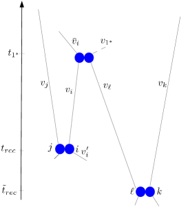
Figure 12. Parallel recollisions.

Lemma B.2.

Fix a final configuration of bounded energy $z_{1}\in\mathbb{T}^{2}\times B_{R}$ with $1\leq R^{2}\leq C_{0}|\log{\varepsilon}|$, a time $1\leq t\leq C_{0}|\log{\varepsilon}|$ and a collision tree $a\in\mathcal{A}_{s}$ with $s\geq 2$.

There exist sets of bad parameters $\mathcal{P}_{2}(a,p,\sigma)\subset\mathcal{T}_{2,s}\times{\mathbb{S}}^{s-1}\times\mathbb{R}^{2(s-1)}$ for $p_{1}<p\leq p_{2}$ and $\sigma\subset\{2,\dots,s\}$ of cardinal $|\sigma|\leq 5$ such that

• $\mathcal{P}_{2}(a,p,\sigma)$ is parametrized only in terms of $(t_{m},v_{m},\nu_{m})$ for $m\in\sigma$ and $m<\min\sigma$;

  (B.31) $$\int{\bf 1}_{\mathcal{P}_{2}(a,p,\sigma)}\displaystyle\prod_{m\in\sigma}\,\big{|}\big{(}v_{m}-v_{a(m)}(t_{{m}}))\cdot\nu_{{m}}\big{|}dt_{{m}}d\nu_{{m}}dv_{{m}}\leq C(Rt)^{r}s^{2}{\varepsilon}\,,$$

  for some constant $r\geq 1$,

• and any pseudo-trajectory starting from $z_{1}$ at $t$, with total energy bounded by $R^{2}$ and such that the first two recollisions involve two disjoint pairs of particles having the same first parent is parametrized by

  $$(t_{n},\nu_{n},v_{n})_{2\leq n\leq s}\in\bigcup_{p_{1}<p\leq p_{2}}\bigcup_{\sigma}\mathcal{P}_{2}(a,p,\sigma)\,.$$

Proof.

As in the previous section, we suppose from now on that the parameters associated with the first recollision are such that $|\tau_{1}||\bar{v}_{i}-v_{j}|\geq R$. Otherwise, the estimate (B.5) applied with $M=R$ leads to the expected upper bound.

In the following, the parents of $i,j$ will be denoted by the superscript $\ {}^{*}$ and those of $k,\ell$ by the superscript $\tilde{\ }$. Denote by $t_{*}:=\min(t_{2^{*}},t_{\tilde{2}})$ the first time (before $t_{1^{*}}$) when one of the particles $i,j$ or $k$ has been deviated. Without loss of generality (up to exchanging $j$ and $k$), we can assume that $i$ and $k$ are not colliding together at time $t_{*}$.

We describe the recollision between $(i,j)$ by the identity

(B.32) $$v_{i}-v_{j}=\frac{1}{t_{rec}-t_{1^{*}}}\big{(}x_{i}(t_{1^{*}})-x_{j}(t_{1^{*}})+q+{\varepsilon}\nu_{rec}\big{)}\,,$$

with $q$ an element in $\mathbb{Z}^{2}$ which we fix from now on (in the end the estimates will be multiplied by $R^{2}t^{2}$ to take this fact into account). Similarly the recollision between $(k,\ell)$ can be written

(B.33) $$v_{\ell}-v_{k}=\frac{1}{\tilde{t}_{rec}-t_{1^{*}}}\big{(}x_{i}(t_{1^{*}})+{\varepsilon}\nu_{1^{*}}-x_{k}(t_{1^{*}})+\tilde{q}+{\varepsilon}\tilde{\nu}_{rec}\big{)}$$

with $\tilde{q}$ an element in $\mathbb{Z}^{2}$ which again we fix from now on, up to mutiplying again the estimates by $R^{2}t^{2}$ at the end.

We introduce the notation

$$\tilde{x}_{i,k}(t_{1^{*}}):=x_{i}(t_{1^{*}})-x_{k}(t_{1^{*}})+\tilde{q}\quad\mbox{and}\quad x_{i,j}(t_{1^{*}}):=x_{i}(t_{1^{*}})-x_{j}(t_{1^{*}})+q\,.$$

Equation (B.32) implies that $v_{i}-v_{j}$ lies in a rectangle $\mathcal{R}_{1}$ of main axis $x_{i,j}(t_{1^{*}})$, and of size $CR\times(R{\varepsilon}/|x_{i,j}(t_{1^{*}})|)$. We recall that an integration of this constraint in the collision parameters of particle $1^{*}$ gives a bound of the type $\min(1,{\varepsilon}|\log{\varepsilon}|^{2}/|\bar{v}_{i}-v_{j}|)$. On the other hand, Equation (B.33) implies that $v_{\ell}-v_{k}$ lies in a rectangle $\mathcal{R}_{2}$ of main axis $\tilde{x}_{i,k}(t_{1^{*}})$ and of size $CR\times(R{\varepsilon}/|\tilde{x}_{i,k}(t_{1^{*}})|)$.

Let us give the main ideas of the argument. We can rewrite these conditions with Carleman’s parametrization (C.9), with either $(v_{i},v_{\ell})=(V^{\prime},V^{\prime}_{*})$ or $(v_{i},v_{\ell})=(V^{\prime}_{*},V^{\prime})$. We will actually focus on the second situation which is the worst one. We will use the parametrization in polar coordinates as in Figure 10.

The first condition states that $V^{\prime}_{*}$ lies in a small rectangle of size $CR\times(R{\varepsilon}/|x_{i,j}(t_{1^{*}})|)$, which we shall eventually integrate with the measure $d\mu d\psi$. We can show that this integral provides a contribution $(R{\varepsilon}/|x_{i,j}(t_{1^{*}})|)(1+|\log({\varepsilon}/|x_{i,j}(t_{1^{*}})|)|)$.

The second condition tells us that $V^{\prime}$ has to be in the intersection of the line orthogonal to $(V^{\prime}_{*}-\bar{v}_{i})$ passing through $\bar{v}_{i}$ and the rectangle $v_{k}+\mathcal{R}_{2}$. We have therefore to evaluate the length of this intersection which appears when we integrate with respect to $\lambda d\lambda$.

Figure 13. The dashed line represents the main axis of the rectangle $\mathcal{R}_{2}$, oriented in the direction $\tilde{x}_{i,k}(t_{1^{*}})$. The angle $\theta$ is the smallest angle between the axis of $\mathcal{R}_{2}$ and any line passing through $v_{i}$ and intersecting the axis of $\mathcal{R}_{2}$.

Denote by $u$ the distance from $\bar{v}_{i}$ to the rectangle $v_{k}+\mathcal{R}_{2}$ :

$$u:=\big{|}(\bar{v}_{i}-v_{k})\wedge\tilde{x}_{i,k}(t_{1^{*}})|/|\tilde{x}_{i,k}(t_{1^{*}})|\,$$

• if this distance is large enough, we expect the length of the intersection to be small;

• if the distance $u$ is small, this imposes an additional constraint on $\bar{v}_{i}-v_{k}$, that we will analyse with different arguments depending on the size of $\tilde{x}_{i,k}(t_{1^{*}})$.

Case $u\geq{\varepsilon}^{3/4}$

The intersection of the line orthogonal to $(V^{\prime}_{*}-\bar{v}_{i})$ passing through $\bar{v}_{i}$ and the rectangle $v_{k}+\mathcal{R}_{2}$ of width $\frac{CR{\varepsilon}}{|\tilde{x}_{i,k}(t_{1^{*}})|}$ (see Figure 13) is a segment of size at most

(B.34) $$d\leq\min\Big{(}\frac{C{\varepsilon}R}{|\tilde{x}_{i,k}(t_{1^{*}})|\sin\theta},CR\Big{)},$$

where $\theta$ is the minimal angle between the axis of $\mathcal{R}_{2}$ and any line passing through $\bar{v}_{i}$ and intersecting $v_{k}+\mathcal{R}_{2}$. We have

$$\sin\theta\geq\frac{u}{2R}\geq\frac{{\varepsilon}^{\frac{3}{4}}}{2R}\,\cdotp$$

It follows from (B.34) that

$$d\leq\frac{C{\varepsilon}^{\frac{1}{4}}R^{2}}{|\tilde{x}_{i,k}(t_{1^{*}})|}\,\cdotp$$

Multiplying this estimate by the size of $\mathcal{R}_{1}$, we get the following upper bound for the measure in $|(v_{1^{*}}-\bar{v}_{i})\cdot\nu_{1^{*}}|\,dv_{1^{*}}d\nu_{1^{*}}$

$$\frac{CR^{5}{\varepsilon}^{\frac{5}{4}}|\log{\varepsilon}|}{\,\big{|}\tilde{x}_{i,k}(t_{1^{*}})\big{|}\,\big{|}x_{i,j}(t_{1^{*}})\big{|}}\big{(}1+\big{|}\log\frac{{\varepsilon}}{|x_{i,j}(t_{1^{*}})|}\big{|}\big{)}\,\cdotp$$

$\bullet$ If $|\tilde{x}_{i,k}(t_{1^{*}})\big{|}\geq{\varepsilon}^{1/8}$ then the bound becomes

$$\frac{CR^{5}{\varepsilon}^{\frac{9}{8}}|\log{\varepsilon}|}{\big{|}x_{i,j}(t_{1^{*}})\big{|}}\,,$$

and we are back to the usual computations as in the proof of Proposition 3.5: we integrate over $t_{1^{*}}$ then over one parent of $(i,j)$ to kill the singularity at small relative velocities, and this gives rise in the end to

$$CR^{5}(R^{3}t)^{2}{\varepsilon}^{\frac{9}{8}}|\log{\varepsilon}|^{3}\,.$$

$\bullet$ If $|\tilde{x}_{i,k}(t_{1^{*}})\big{|}\leq{\varepsilon}^{1/8}$, we have a kind of “recollision” between particles $i$ and $k$ at time $t_{1}^{*}$. Denote by $\tilde{2},\tilde{3}$ the first two parents of $(i,k)$. We therefore get that $\bar{v}_{i}-v_{k}$ has to belong to the union of $(Rt)^{2}$ rectangles $\mathcal{R}_{3}$ of size $CR\times(R{\varepsilon}^{1/8}/|\tilde{x}_{i,k}(t_{\tilde{2}})|)$, with

$$\tilde{x}_{i,k}(t_{\tilde{2}}):=x_{i}(t_{\tilde{2}})-x_{k}(t_{\tilde{2}})+\tilde{q}\,.$$

Combined with the condition that $v_{i}\in\mathcal{R}_{1}$, one has to integrate

$$R^{3}{\bf 1}_{\{\bar{v}_{i}-v_{k}\in\mathcal{R}_{3}\}}\min\left({{\varepsilon}\,|\log{\varepsilon}|^{2}\over|\bar{v}_{i}-v_{j}|},1\right).$$

Denote by $\sigma=\{1^{*},2^{*},3^{*}\}\cup\{\tilde{2},\tilde{3}\}$ so that the cardinal $|\sigma|$ can be 3, 4 or 5. Integrating over $1^{*}$ leads to an inequality involving constraints on the pairs $(i,k)$ and $(i,j)$

$$\int{\bf 1}_{\{\bar{v}_{i}-v_{k}\in\mathcal{R}_{3}\}}{\bf 1}_{\{v_{i}-v_{j}\in\mathcal{R}_{1}\}}\,\prod_{m\in\sigma}b(\nu_{m},v_{m})\,dv_{m}d\nu_{m}dt_{m}$$

$$\qquad\leq R^{3}{\varepsilon}|\log{\varepsilon}|^{2}\int\frac{{\bf 1}_{\{\bar{v}_{i}-v_{k}\in\mathcal{R}_{3}\}}}{|\bar{v}_{i}-v_{j}|}\,\prod_{m\in\{2^{*},3^{*},\tilde{2},\tilde{3}\}}b(\nu_{m},v_{m})\,dv_{m}d\nu_{m}dt_{m}$$

(B.35) $$\qquad\leq R^{3}{\varepsilon}|\log{\varepsilon}|^{2}\left((R^{3}t)^{2}\int{\bf 1}_{\{\bar{v}_{i}-v_{k}\in\mathcal{R}_{3}\}}\prod_{m=\tilde{2},\tilde{3}}b(\nu_{m},v_{m})\,dv_{m}d\nu_{m}dt_{m}\right)^{1/4}$$

$$\qquad\qquad\qquad\times\left((R^{3}t)^{2}\int\frac{1}{|\bar{v}_{i}-v_{j}|^{4/3}}\prod_{m=2^{*},3^{*}}b(\nu_{m},v_{m})\,dv_{m}d\nu_{m}dt_{m}\right)^{3/4}$$

$$\qquad\leq C(Rt)^{r}{\varepsilon}^{33/32}|\log{\varepsilon}|^{11/4}\,,$$

where we used Hölder’s inequality in order to decouple both terms: the first one provides as previously a bound ${\varepsilon}^{\frac{1}{8}}|\log{\varepsilon}|^{3}$ and the second one is bounded thanks to (C.6)-(C.7) as the singularity in the relative velocities is less than 2. Note that Hölder’s inequality was performed over the 4 variables $\{2^{*},3^{*},\tilde{2},\tilde{3}\}$, but only two variables are relevant for each integral, thus the contribution of the two others is bounded from above by the factor $(R^{3}t)^{2}$.

Case $u\leq{\varepsilon}^{3/4}$

We recall that

$$\tilde{x}_{i,k}(t_{1^{*}}) :=x_{i}(t_{1^{*}})-x_{k}(t_{1^{*}})+\tilde{q}=x_{i}(t_{\tilde{2}})-x_{k}(t_{\tilde{2}})+\tilde{q}+(\bar{v}_{i}-v_{k})(t_{1^{*}}-t_{\tilde{2}})\,.$$

Recalling that

$$\tilde{x}_{i,k}(t_{\tilde{2}}):=x_{i}(t_{\tilde{2}})-x_{k}(t_{\tilde{2}})+\tilde{q}\,,$$

the constraint $u=\frac{|(\bar{v}_{i}-v_{k})\wedge\tilde{x}_{i,k}(t_{1^{*}})|}{|\tilde{x}_{i,k}(t_{1^{*}})|}\leq{\varepsilon}^{\frac{3}{4}}$ implies

(B.36) $$\big{|}(\bar{v}_{i}-v_{k})\wedge\tilde{x}_{i,k}(t_{\tilde{2}})\big{|}\leq C{\varepsilon}^{\frac{3}{4}}Rt\,.$$

Recall that the constraint (B.32) on the rectangle ${\mathcal{R}}_{1}$ produces a singularity $\frac{R{\varepsilon}}{|x_{i,j}(t_{1^{*}})|}(1+|\log(\frac{{\varepsilon}}{|x_{i,j}(t_{1^{*}})|})|)$, and we argue as follows:

$\bullet$ If $|\tilde{x}_{i,k}(t_{\tilde{2}})|\leq{\varepsilon}^{\frac{5}{8}}$, we have a kind of “recollision” between particles $i$ and $k$ at time $t_{\tilde{2}}$. We thus proceed as in Case 1 of Section 6.

- For small relative velocities, we integrate the constraint $|\bar{v}_{i}-v_{j}|\leq{\varepsilon}^{\frac{9}{16}}$ over two parents of $\{i,j\}$ using (C.3), (C.4) and we find directly a bound ${\varepsilon}^{\frac{9}{8}}|\log{\varepsilon}|^{2}$.

- When the relative velocities are bounded from below $|\bar{v}_{i}-v_{j}|\geq{\varepsilon}^{\frac{9}{16}}$, the contribution of rectangle ${\mathcal{R}}_{1}$ gives a bound of the order $CR^{2}{\varepsilon}^{\frac{7}{16}}|\log{\varepsilon}|^{2}$. By integrating the “recollision” $(i,k)$ over $\tilde{2},\tilde{3}$, we find a bound $CR^{7}t^{3}{\varepsilon}^{\frac{5}{8}}|\log{\varepsilon}|^{3}$ so finally this case produces as usual (see Proposition 3.5), after integration over three parameters, the error $CR^{9}t^{3}{\varepsilon}^{\frac{17}{16}}|\log{\varepsilon}|^{5}$.

$\bullet$ If  $|\tilde{x}_{i,k}(t_{\tilde{2}})|\geq{\varepsilon}^{\frac{5}{8}}$ then according to (B.36), $\bar{v}_{i}-v_{k}$ must lie in the union of $(Rt)^{2}$ rectangles ${\mathcal{R}}_{4}$ with axis $\tilde{x}_{i,k}(t_{\tilde{2}})$ and size $CR\times CRt{\varepsilon}^{\frac{1}{8}}$. This condition has to be coupled with the singularity ${\varepsilon}|\log{\varepsilon}|^{2}/|\bar{v}_{i}-v_{j}|$ due to the constraint from the rectangle $\mathcal{R}_{1}$. We therefore have to integrate

$$R^{3}{\bf 1}_{\{\bar{v}_{i}-v_{k}\in\mathcal{R}_{4}\}}\min\left({{\varepsilon}|\log{\varepsilon}|^{2}\over|\bar{v}_{i}-v_{j}|},1\right).$$

Denote by $\sigma=\{1^{*},2^{*},3^{*}\}\cup\{\tilde{2}\}$ where $\tilde{2}$ is the first parent of $(i,k)$. In this case, the cardinal of $\sigma$ is 3 or 4. Integrating first over $1^{*}$ and then using Hölder’s inequality as in (B.3), we have

$$\int{\bf 1}_{\{\bar{v}_{i}-v_{k}\in\mathcal{R}_{4}\}}{\bf 1}_{\{v_{i}-v_{j}\in\mathcal{R}_{1}\}}\,\prod_{m\in\sigma}b(\nu_{m},v_{m})\,dv_{m}d\nu_{m}dt_{m}$$

$$\qquad\leq R^{3}{\varepsilon}|\log{\varepsilon}|^{2}\int{{\bf 1}_{\{\bar{v}_{i}-v_{k}\in\mathcal{R}_{4}\}}\over|\bar{v}_{i}-v_{j}|}\,\prod_{m\in\sigma\setminus\{1^{*}\}}b(\nu_{m},v_{m})\,dv_{m}d\nu_{m}dt_{m}$$

$$\qquad\leq R^{3}{\varepsilon}|\log{\varepsilon}|^{2}\left((R^{3}t)^{2}\int{\bf 1}_{\{\bar{v}_{i}-v_{k}\in\mathcal{R}_{4}\}}b(\nu_{\tilde{2}},v_{\tilde{2}})\,dv_{\tilde{2}}d\nu_{\tilde{2}}dt_{\tilde{2}}\right)^{1/4}$$

$$\qquad\qquad\qquad\times\left((R^{3}t)\int\frac{1}{|\bar{v}_{i}-v_{j}|^{4/3}}\prod_{m=2^{*},3^{*}}b(\nu_{m},v_{m})\,dv_{m}d\nu_{m}dt_{m}\right)^{3/4}$$

$$\qquad\leq C(Rt)^{r}{\varepsilon}^{33/32}|\log{\varepsilon}|^{9/4}\,.$$

Given a set $\sigma$ of parents, it may only determine the particle $i$, so that an extra factor $s^{2}$ has to be added in (B.31) to take into account the choice of $j,k$. This completes the proof of Lemma B.2. ∎

B.4. Recollisions in chain

The following Lemma was used in Section 6.2.2 page 6.2.2 to deal with the case when recollisions occur in chain, with $t_{\tilde{1}}=t_{1^{*}}$, i.e. both recollisions occur without any intermediate collisions as depicted in Figure 14.

Figure 14. Recollisions in chain.

Lemma B.3.

Fix a final configuration of bounded energy $z_{1}\in\mathbb{T}^{2}\times B_{R}$ with $1\leq R^{2}\leq C_{0}|\log{\varepsilon}|$, a time $1\leq t\leq C_{0}|\log{\varepsilon}|$ and a collision tree $a\in\mathcal{A}_{s}$ with $s\geq 2$.

There exist sets of bad parameters $\mathcal{P}_{2}(a,p,\sigma)\subset\mathcal{T}_{2,s}\times{\mathbb{S}}^{s-1}\times\mathbb{R}^{2(s-1)}$ for $p_{2}<p\leq p_{3}$ and $\sigma\subset\{2,\dots,s\}$ of cardinal $|\sigma|\leq 3$ such that

• $\mathcal{P}_{2}(a,p,\sigma)$ is parametrized only in terms of $(t_{m},v_{m},\nu_{m})$ for $m\in\sigma$ and $m<\min\sigma$;

  (B.37) $$\int{\bf 1}_{\mathcal{P}_{2}(a,p,\sigma)}\displaystyle\prod_{m\in\sigma}\,\big{|}\big{(}v_{m}-v_{a(m)}(t_{{m}}))\cdot\nu_{{m}}\big{|}dt_{{m}}d\nu_{{m}}dv_{{m}}\leq C(Rt)^{r}s^{2}{\varepsilon}\,,$$

  for some constant $r\geq 1$,

• and any pseudo-trajectory starting from $z_{1}$ at $t$, with total energy bounded by $R^{2}$ and such that the first two recollisions occur in chain as in Figure 14 is parametrized by

  $$(t_{n},\nu_{n},v_{n})_{2\leq n\leq s}\in\bigcup_{p_{2}<p\leq p_{3}}\bigcup_{\sigma}\mathcal{P}_{2}(a,p,\sigma)\,.$$

Proof.

Recall that the condition for the first recollision states

(B.38) $$v_{i}-v_{j}=\frac{1}{\tau_{rec}}\delta x_{\perp}-\frac{\tau_{1}}{\tau_{rec}}(\bar{v}_{i}-v_{j})-\frac{1}{\tau_{rec}}\nu_{rec}\,,$$

with $x_{i},x_{j}$ the positions at time $t_{2^{*}}$

(B.39) $$\delta x :=\frac{1}{{\varepsilon}}(x_{i}-x_{j}-q)=\lambda(\bar{v}_{i}-v_{j})+\delta x_{\perp}\qquad\hbox{with}\quad\delta x_{\perp}\cdot(\bar{v}_{i}-v_{j})=0\,,$$

$$\tau_{1} :=\frac{1}{{\varepsilon}}(t_{1^{*}}-t_{2^{*}}-\lambda)\,,\qquad\tau_{rec}:=\frac{1}{{\varepsilon}}(t_{rec}-t_{1^{*}})\,,$$

for some $q$ in $\mathbb{Z}^{2}$ of norm smaller than $O(Rt)$ to take into account the periodicity.

When $|\tau_{1}||\bar{v}_{i}-v_{j}|\leq R^{2}$, estimate (B.5) is enough to obtain an upper bound of order ${\varepsilon}$ without taking into account the second recollision. Our goal here is to prove that the constraint of having a second recollision produces an integrable function of $|\tau_{1}|\,|\bar{v}_{i}-v_{j}|\geq R^{2}$, hence a bound $O({\varepsilon})$ after integration over $1^{*}$.

From (B.38), we deduce as in (3.10) that

(B.40) $$\frac{1}{|\tau_{rec}|}\leq{4R\over|\tau_{1}||\bar{v}_{i}-v_{j}|}\quad\text{which implies that}\quad|\tau_{rec}|\geq R/4\gg 1\,.$$

Two cases have to be considered: $k=1^{*}$ and $k\neq 1^{*}$.

Case $k=1^{*}$.

The equation for the second recollision states

$$\tau^{\prime}_{rec}(v^{\prime}_{i}-{v_{1^{*}}^{\prime}})=\pm\nu_{1^{*}}-\tau_{rec}(v_{i}-{v_{1^{*}}^{\prime}})(+\nu_{rec})-\tilde{\nu}_{rec},$$

where

$$\tau^{\prime}_{rec}:=\frac{1}{{\varepsilon}}(\tilde{t}_{rec}-t_{rec})\,,$$

and where the $\pm$ and the translation by $\nu_{rec}$ depend on the possible exchanges in the labels of the particles at collision times. It can be rewritten, thanks to (B.10),

(B.41) $$\tau^{\prime}_{rec}(v_{j}-v_{i})\cdot\nu_{rec}\,\nu_{rec} =\pm\nu_{1^{*}}-(\tau_{rec}+\tau^{\prime}_{rec})(v_{i}-{v^{\prime}_{1^{*}}})(+\nu_{rec})-\tilde{\nu}_{rec}$$

$$\hbox{ or }\qquad\tau^{\prime}_{rec}(v_{j}-v_{i})\cdot\nu_{rec}^{\perp}\,\nu_{rec}^{\perp} =\pm\nu_{1^{*}}-(\tau_{rec}+\tau^{\prime}_{rec})(v_{i}-{v^{\prime}_{1^{*}}})(+\nu_{rec})-\tilde{\nu}_{rec}\,.$$

We further know that $|v_{i}-{v^{\prime}_{1^{*}}}|=|\bar{v}_{i}-v_{1^{*}}|$.

- If $|\bar{v}_{i}-v_{1^{*}}|\geq R\,|\tau_{rec}|^{-3/4}$, then the vector in the right-hand side of (B.41) has a magnitude of order

$$|\tau_{rec}+\tau^{\prime}_{rec}|\,|v_{i}-{v^{\prime}_{1^{*}}}|\geq|\tau_{rec}|\,|v_{i}-{v^{\prime}_{1^{*}}}|\geq R\,|\tau_{rec}|^{1/4}\,.$$

It follows that the vector $\nu_{rec}$ has to be aligned in the direction of $v_{i}-v_{1^{*}}^{\prime}$ with a controlled error

$$\nu_{rec}=\mathcal{R}_{n\pi/2}{v_{i}-{v_{1^{*}}^{\prime}}\over|\bar{v}_{i}-v_{1^{*}}|}+O\left({1\over|\tau_{rec}|^{1/4}}\right)\,,$$

for $n=0,1,2,3$, recalling that $\mathcal{R}_{\theta}$ is the rotation of angle $\theta$.

Plugging the formula for $\nu_{rec}$ into (B.38) and using (B.40), we get

$$v_{i}-v_{j}=\frac{1}{\tau_{rec}}\delta x_{\perp}-\frac{\tau_{1}}{\tau_{rec}}(\bar{v}_{i}-v_{j})-\frac{1}{\tau_{rec}}\mathcal{R}_{n\pi/2}{v_{i}-{v_{1^{*}}^{\prime}}\over|\bar{v}_{i}-v_{1^{*}}|}+O\left({R^{5/4}\over|\tau_{1}|^{5/4}\;|\bar{v}_{i}-v_{j}|^{5/4}}\right)\,.$$

This equation has the same structure as (B.13). Thus using the same arguments as in the proof of Lemma B.1, we get

• a contribution of size $O(|\tau_{1}|^{-5/4}\;|\bar{v}_{i}-v_{j}|^{-5/4}|\log|\tau_{1}(\bar{v}_{i}-v_{j})|)$ when the mapping $v_{i}\mapsto{v_{i}-v_{1^{*}}^{\prime}\over|v_{i}-v_{1^{*}}^{\prime}|}$ is Lipschitz with constant strictly less than $|w|^{\gamma}$ for some $\gamma\in(0,1)$;

• the same integrable contribution as in Lemma B.1 in degenerate cases when some velocities are close to each other (typically at a distance $O(|w|^{-\gamma})$).

Thus integrating with respect to $t_{1^{*}}$ we recover the factor ${\varepsilon}$ and the singularity in $|\bar{v}_{i}-v_{j}|$ is removed as usual by integration over the parents of $i,j$.

- If $|\bar{v}_{i}-v_{1^{*}}|\leq R|\tau_{rec}|^{-3/4}$, we find that $v_{1^{*}}$ has to belong to a domain of size less than $(|\tau_{1}|\,|\bar{v}_{i}-v_{j}|)^{-3/2}$ as $|\tau_{rec}|\geq|\tau_{1}|\,|\bar{v}_{i}-v_{j}|$. Hence again, we obtain an integrable function of $|\tau_{1}|\,|\bar{v}_{i}-v_{j}|$, with no extra gain in ${\varepsilon}$.

Case $k\neq 1^{*}$. In the following we denote by $1^{*},2^{*}\dots$ the parents of the set $(i,j,k,\ell)$ at time $t_{rec}$: contrary to previous cases, and since they both have the same first parent we do not distinguish the parents of $(i,j)$ and $(k,\ell)$ but consider them as a whole.

The position of particle $k$ at the time $\tilde{t}_{rec}$ of the second recollision is given by

$$x_{k}(t_{rec})=x_{k}+v_{k}(\tilde{t}_{rec}-t_{2^{*}})\,.$$

We have written $x_{k}$ for the position of particle $k$ at time $t_{2^{*}}$. We end up with the condition for the second recollision

(B.42) $$(\tilde{t}_{rec}-t_{rec})(v^{\prime}_{i}-v_{k})=(x_{j}-x_{k})(t_{rec})-{\varepsilon}\tilde{\nu}_{rec}(+{\varepsilon}\nu_{rec})+\tilde{q}\,,$$

for some $\tilde{q}\in\mathbb{Z}^{2}$ not larger than $O(Rt)$, and where the translation ${\varepsilon}\nu_{rec}$ arises only if the labels of particles are exchanged at $t_{rec}$. In the following, we fix $q$ and $\tilde{q}$ and will multiply the final estimate by $(R^{2}t^{2})^{2}$ to take into account the periodicity in both recollisions. Using the notation (B.39), we then rescale in ${\varepsilon}$ and write

$$\tau_{rec}:=\frac{t_{rec}-t_{1^{*}}}{{\varepsilon}}\,,\quad\tau^{\prime}_{rec}:=\frac{\tilde{t}_{rec}-t_{rec}}{{\varepsilon}}\,\cdotp$$

Then Equation (B.42) for the second recollision becomes

(B.43) $$\tau^{\prime}_{rec}(v^{\prime}_{i}-v_{k})=\tilde{x}_{jk}(t_{rec})-\tilde{\nu}_{rec}(+\nu_{rec})\,,$$

where ${\varepsilon}\tilde{x}_{jk}(t_{rec})$ stands for the relative position between $j,k$ at time $t_{rec}$.

As in the proof of Lemma 3.7, the equation (B.43) implies that $v^{\prime}_{i}-v_{k}$ belongs to a rectangle $\mathcal{R}$ of size $2R\times\frac{2R}{|\tilde{x}_{jk}(t_{rec})|}$ and axis $\tilde{x}_{jk}(t_{rec})$. Furthermore $v^{\prime}_{i}$ belongs as well to the circle of diameter $[v_{j},v_{i}]$ by definition. Computing the intersection of the rectangle and of the circle, we obtain a constraint on the angle $\nu_{rec}$. Then plugging this constraint in the equation for the first recollision, we will conclude as in Lemma B.1 that $v_{i}$ has to belong to a very small set.

Figure 15. The velocity $v_{i}^{\prime}$ belongs to the rectangle of axis $\tilde{x}_{jk}(t_{rec})$ as well as to the circle of diameter $[v_{j},v_{i}]$.

This strategy can be applied in most situations. We have however to deal separately with the two following geometries :

• if the relative velocity $v_{i}-v_{j}$ is small, the rectangle can contain a macroscopic part of the circle : we forget about the second recollision and just study the constraint of small relative velocities;

• if the distance $|\tilde{x}_{jk}(t_{rec})|$ is small, then $i$ will be close to $k$ at the first recollision time and this will facilitate the second recollision : we then forget about the second recollision and write two independent constraints at the first recollision time.

$\bullet$ Suppose that

(B.44) $$|v_{i}-v_{j}|\geq{1\over|\tau_{rec}|^{5/8}}\quad\text{and}\quad|\tilde{x}_{jk}(t_{rec})|\geq|\tau_{rec}|^{3/4}.$$

From (B.43), we deduce that a necessary condition for the second recollision to hold is that

$$(v_{i}^{\prime}-v_{k})\cdot{\tilde{x}_{jk}^{\perp}(t_{rec})\over|\tilde{x}_{jk}(t_{rec})|}={(v_{i}-\big{(}(v_{i}-v_{j})\cdot\nu_{rec}\big{)}\,\nu_{rec}-v_{k})\cdot\tilde{x}_{jk}^{\perp}(t_{rec})\over|\tilde{x}_{jk}(t_{rec})|}=O\Big{(}{1\over|\tau^{\prime}_{rec}|}\Big{)},$$

where $|\tau^{\prime}_{rec}|$ can be bounded from below thanks to (B.44)

$$|\tau^{\prime}_{rec}|\geq{|\tilde{x}_{jk}(t_{rec})|\over 4R}\geq{|\tau_{rec}|^{3/4}\over 4R}\,.$$

Using the bound from below on the relative velocity $|v_{i}-v_{j}|$, we finally get

$$\Big{(}{v_{i}-v_{j}\over|v_{i}-v_{j}|}\cdot\nu_{rec}\Big{)}\Big{(}{\tilde{x}_{jk}^{\perp}(t_{rec})\over|\tilde{x}_{jk}(t_{rec})|}\cdot\nu_{rec}\Big{)}={(v_{i}-v_{k})\cdot\tilde{x}_{jk}^{\perp}(t_{rec})\over|v_{i}-v_{j}||\tilde{x}_{jk}^{\perp}(t_{rec})|}+O\Big{(}{1\over|\tau_{rec}|^{1/8}}\Big{)}\,.$$

Define the angles $\theta=<\tilde{x}_{jk}^{\perp}(t_{rec}),\nu_{rec}>$ and $\alpha=<\tilde{x}_{jk}^{\perp}(t_{rec}),v_{i}-v_{j}>$. We have

$$\cos\theta\cos(\theta-\alpha)=\frac{1}{2}\Big{(}\cos(2\theta-\alpha)+\cos\alpha\Big{)}={(v_{i}-v_{k})\cdot\tilde{x}_{jk}^{\perp}(t_{rec})\over|v_{i}-v_{j}||\tilde{x}_{jk}^{\perp}(t_{rec})|}+O\Big{(}{1\over|\tau_{rec}|^{1/8}}\Big{)},$$

so that

$$\cos(2\theta-\alpha)={(v_{i}+v_{j}-2v_{k})\cdot\tilde{x}_{jk}^{\perp}(t_{rec})\over|v_{i}-v_{j}||\tilde{x}_{jk}^{\perp}(t_{rec})|}+O\Big{(}{1\over|\tau_{rec}|^{1/8}}\Big{)}.$$

Recall the notation of the proof of Lemma B.1

$$w:=\delta x^{\perp}_{i,j}-(\bar{v}_{i}-v_{j})\tau_{1},\quad\text{ and}\quad u:={|w|\over\tau_{rec}}\leq 4R,$$

where ${\varepsilon}w$ is the distance between $x_{i},x_{j}$ at time $t_{1^{*}}$ and it is enough to consider $|w|\geq R^{2}$ thanks to (B.5). As the derivative of $\arccos$ is singular at $\pm 1$, we will consider an approximation $\arccos_{|w|}$ which coincides with $\arccos$ on $[-1+\frac{1}{|w|^{2\delta}},1-\frac{1}{|w|^{2\delta}}]$ (for a given $\delta\in(0,\frac{1}{16})$) and is constant in the rest of $[-1,1]$ so that

$$\big{|}\partial_{x}\arccos_{|w|}(x)\big{|}\leq|w|^{\delta}\quad\text{and}\quad\|\arccos_{|w|}-\arccos\|_{\infty}\leq\frac{1}{|w|^{\delta}}.$$

Thus the angle $\theta$ can be approximated by

$$\theta=\bar{\theta}_{\pm}+O\Big{(}\left(\frac{u}{|w|}\right)^{1/8}|w|^{\delta}+\frac{1}{|w|^{\delta}}\Big{)},$$

with

(B.45) $$\bar{\theta}_{\pm}=\pm\frac{1}{2}\arccos_{|w|}\left({(v_{i}+v_{j}-2v_{k})\cdot\tilde{x}_{jk}^{\perp}(t_{rec})\over|v_{i}-v_{j}||\tilde{x}_{jk}^{\perp}(t_{rec})|}\right)+\frac{1}{2}<\tilde{x}_{jk}^{\perp}(t_{rec}),v_{i}-v_{j}>.$$

Plugging this constraint in the equation for the first recollision, we get

(B.46) $$v_{i}-v_{j}=u{w\over|w|}-{u\over|w|}\mathcal{R}_{\bar{\theta}_{\pm}}{\tilde{x}_{jk}^{\perp}(t_{rec})\over|\tilde{x}_{jk}(t_{rec})|}+O\Big{(}u^{\delta}\left(\frac{u}{|w|}\right)^{9/8-\delta}+\frac{u}{|w|}\,\frac{1}{|w|^{\delta}}\Big{)}.$$

As $|w|\gg 1$, the leading term of this equation is $v_{i}-v_{j}\simeq u{w\over|w|}$, but we have to analyse carefully the corrections. Compared with the formulas of the same type encountered in the proof of Lemma B.1, this one has the additional difficulty that the dependence with respect to $u$ is very intricate. Instead of solving (B.46), we are going to look at sufficient conditions satisfied by the solutions of (B.46). In particular, $u$ will be considered as a parameter independent of $|\tau_{rec}|$. For a given $u$, we are going to solve the equation

(B.47) $$v_{i}-v_{j}=u{w\over|w|}-{u\over|w|}\mathcal{R}_{\bar{\theta}_{\pm}}{\tilde{x}_{jk}^{\perp}(t_{rec})\over|\tilde{x}_{jk}(t_{rec})|}\quad\text{with}\quad|v_{i}-v_{j}|\geq\frac{1}{2}\left({u\over|w|}\right)^{5/8},$$

where $\tilde{x}_{jk}(t_{rec})$ was originally defined in (B.43) as the relative position between $j,k$ at time $t_{rec}$, but is now simply a function of $u$

$$\tilde{x}_{jk}(t_{rec})=x_{jk}(t_{1^{*}})-{|w|\over u}(v_{j}-v_{k}).$$

The solutions of (B.46) are such that $u\simeq|v_{i}-v_{j}|$, thus from the condition (B.47) on the relative velocities, it is enough to restrict the range of the parameter $u$ to $u\geq\frac{1}{4}\left({u\over|w|}\right)^{5/8}$, i.e. $u\in[\frac{1}{4|w|^{5/3}},4R]$. We will first show that for any such $u$, there is a unique solution $\hat{v}_{i}(u)$ of (B.47). The solution of (B.46) will be located close to the curve $u\to\hat{v}_{i}(u)$, thus we will then need to control the regularity of the curve $u\to\hat{v}_{i}(u)$ to estimate the size of the tubular neighborhood around this curve.

- For fixed $u$, note that $\tilde{x}_{jk}^{\perp}(t_{rec})$ is also fixed. The only dependence with respect to $v_{i}$ in the right-hand side of (B.47) is via $\bar{\theta}_{\pm}$ :

$$d\bar{\theta}_{\pm}\leq \frac{1}{2}|w|^{\delta}\,{|v_{i}-v_{j}|^{2}\tilde{x}_{jk}^{\perp}(t_{rec})\cdot dv_{i}-((v_{i}+v_{j}-2v_{k})\cdot\tilde{x}_{jk}^{\perp}(t_{rec}))\;(v_{i}-v_{j})\cdot dv_{i}\over|v_{i}-v_{j}|^{3}|\tilde{x}_{jk}(t_{rec})|}$$

(B.48) $$-\frac{1}{2}d<\tilde{x}_{jk}^{\perp}(t_{rec}),v_{i}-v_{j}>\,.$$

where we used the Lipschitz bound satisfied by $\arccos_{|w|}$. Note that second term in (B.48) controls the variation of the angle $<\tilde{x}_{jk}^{\perp}(t_{rec}),v_{i}-v_{j}>$ and has Lipschitz constant less than $\frac{1}{|v_{i}-v_{j}|}$. Together with the bounds (B.44), this implies that $v_{i}\mapsto\bar{\theta}_{\pm}(v_{i},u)$ is Lipschitz continuous with constant

$$C|w|^{\delta}\;\max\frac{1}{|v_{i}-v_{j}|}\leq C\left({|w|\over u}\right)^{5/8+\delta}u^{\delta}\ll{|w|\over u}.$$

We therefore conclude by Picard’s fixed point theorem that there is a unique solution $\hat{v}_{i}=\hat{v}_{i}(u)$. As $\delta<1/16$, we further have that any solution to (B.46) satisfies

$$v_{i}=\hat{v}_{i}(u)+O\Big{(}u^{\delta}\left(\frac{u}{|w|}\right)^{9/8-\delta}+\frac{u}{|w|}\,\frac{1}{|w|^{\delta}}\Big{)},$$

for $u\in[\frac{1}{4|w|^{5/3}},4R]$.

- Let us now study the regularity of $u\mapsto\hat{v}_{i}(u)$. In (B.47), we have both an explicit dependence with respect to $u$ and a dependence via the direction of $\tilde{x}_{jk}(t_{rec})$. To take into account the condition (B.44), we further restrict the range of $u$ to

(B.49) $$u\in[\frac{1}{4|w|^{5/3}},4R]\quad\text{and}\quad|\tilde{x}_{jk}(t_{rec})|\geq\left({|w|\over u}\right)^{3/4}.$$

The derivative of ${\tilde{x}_{jk}(t_{rec})\over|\tilde{x}_{jk}(t_{rec})|}$ with respect to $u$ is controlled by

(B.50) $${|w||v_{j}-v_{k}|\over u^{2}|\tilde{x}_{jk}(t_{rec})|}\leq C(R)\left({|w|\over u}\right)^{1+5/8-3/4}=C(R)\left({|w|\over u}\right)^{7/8}$$

as $u\geq{1\over 2}\left(u\over{|w|}\right)^{5/8}$ thanks to (B.49). Thus the Lipschitz constant of $u\mapsto\bar{\theta}_{\pm}(v_{i},u)$ is less than $\big{(}|w|/u\big{)}^{7/8}\,|w|^{\delta}$. Gathering both estimates, we finally get by differentiating (B.47) with respect to $v_{i}$ and $u$ that $u\mapsto\hat{v}_{i}(u)$ is Lipschitz continuous with constant $1+C\big{(}|w|/u\big{)}^{-1/8+\delta}u^{\delta}$, which is bounded as $\delta<1/16$. The solutions of (B.46) are at a distance at most ${R\over|w|^{1+\delta}}$ from the curve $u\mapsto\hat{v}_{i}(u)$. Thus under the condition (B.44), any recollision in chain will belong to the tubular neighborhood of $u\mapsto\hat{v}_{i}(u)$.

In order to estimate the measure that $v_{i}$ belongs to this tubular neighborhood, we proceed as in (C.10) and cover this tube by $O(|w|^{1+\delta})$ balls of size ${R\over|w|^{1+\delta}}$. Integrating with respect to $dv_{1^{*}}d\nu_{1^{*}}$, we get an estimate $O\left(\frac{|\log|w||}{|w|^{1+\delta}}\right)$. By construction $|w|\geq|\tau_{1}||\bar{v}_{i}-v_{j}|$ so that the remainder can be integrated with respect to $\tau_{1}$. Changing to the variable $t_{1^{*}}$, we obtain an upper bound of order ${\varepsilon}$. We then kill the singularity $\frac{\big{|}\log|\bar{v}_{i}-v_{j}|\big{|}}{|\bar{v}_{i}-v_{j}|^{1+\delta}}$ at small relative velocities by integrating with respect to two additional parents, applying (C.6) and then (C.7).

$\bullet$ Suppose that $|v_{i}-v_{j}|\leq|\tau_{rec}|^{-5/8}$. We obtain by (C.3) that

(B.51) $$\int{\bf 1}_{\{|v_{i}-v_{j}|\leq|\tau_{rec}|^{-5/8}\}}|(v_{1^{*}}-v_{i})\cdot\nu_{1^{*}}|d\nu_{1^{*}}dv_{1^{*}}$$

$$\qquad\leq\int{\bf 1}_{\{|v_{i}-v_{j}|\leq\frac{1}{|\tau_{1}|^{5/8}\,|\bar{v}_{i}-v_{j}|^{5/8}}\}}|(v_{1^{*}}-v_{i})\cdot\nu_{1^{*}}|d\nu_{1^{*}}dv_{1^{*}}$$

$$\qquad\leq\frac{CR^{2}}{|\tau_{1}|^{5/8}\,|\bar{v}_{i}-v_{j}|^{5/8}}\min\left(\frac{1}{|\tau_{1}|^{5/8}\,|\bar{v}_{i}-v_{j}|^{13/8}},1\right)\leq\frac{CR^{2}}{|\tau_{1}|^{9/8}\,|\bar{v}_{i}-v_{j}|^{77/40}},$$

where in the last inequality, we used that $\min(\delta,1)\leq\delta^{4/5}$. This produces an integrable function of $|\tau_{1}|$ and leads to an upper bound of order ${\varepsilon}$. The singularity in $|\bar{v}_{i}-v_{j}|$ can be integrated out by applying (C.6) and then (C.7) on the parents of $i,j$.

$\bullet$ Suppose that $|\tilde{x}_{j,k}(t_{rec})|\leq|\tau_{rec}|^{3/4}$, this condition can be interpreted as a “kind of recollision” between $j$ and $k$ at time $t_{rec}$. Note that this situation is similar to the last case studied in Lemma B.1, where the size of the error depends on $|\tau_{1}||\bar{v}_{i}-v_{j}|$.

Figure 16. In the case $|\tilde{x}_{j,k}(t_{rec})|\leq|\tau_{rec}|^{3/4}$, we will forget about the recollision between $i,k$ and use instead that $j$ and $k$ are close at time $t_{rec}$.

The first recollision between $i,j$ imposes that $v_{i}-v_{j}$ belongs to a rectangle $\mathcal{R}$. Integrating first the condition for the recollision between $(i,j)$ with respect to $b(\nu_{1^{*}},v_{1^{*}})\,dv_{1^{*}}d\nu_{1^{*}}$, we gain a factor $(\tau_{1}|\bar{v}_{i}-v_{j}|)^{-1}$. We will not use the recollision between $i,k$ and focus on the additional constraint that the distance between $j,k$ is less than ${\varepsilon}|\tau_{rec}|^{3/4}$ at time $t_{rec}$.

Denote by $\tilde{1}$ the first parent of $(j,k)$. By analogy with equation (B.1), the constraint $|\tilde{x}_{j,k}(t_{rec})|\leq|\tau_{rec}|^{3/4}$ reads

$$(x_{j}-x_{k})(t_{\tilde{1}})+(t_{rec}-t_{\tilde{1}})(v_{j}-v_{k})={\varepsilon}\eta+q,$$

with $|\eta|\leq|\tau_{rec}|^{3/4}$ and a given $q\in\mathbb{Z}^{2}$ with modulus less than $Rt$. With the notation $\tilde{\tau}_{rec}=\frac{t_{rec}-t_{\tilde{1}}}{{\varepsilon}}$, this can be rewritten

(B.52) $$v_{j}-v_{k}=\frac{(x_{j}-x_{k})(t_{\tilde{1}}+q)}{{\varepsilon}\tilde{\tau}_{rec}}+\frac{\eta}{\tilde{\tau}_{rec}}.$$

Since $\tilde{\tau}_{rec}\geq\tau_{rec}$, we get

$$\frac{\eta}{|\tilde{\tau}_{rec}|}\leq\frac{1}{|\tau_{rec}|^{1/4}}\leq\frac{1}{(|\tau_{1}||\bar{v}_{i}-v_{j}|)^{1/4}},$$

so that $v_{j}-v_{k}$ has to belong to a rectangle $\tilde{\mathcal{R}}$ of width less than $\frac{1}{(|\tau_{1}||\bar{v}_{i}-v_{j}|)^{1/4}}$.

As in the last case of Lemma B.1, we split the proof according to the size of $|\tau_{1}|$.

- If $|\tau_{1}|\geq{1\over|\bar{v}_{i}-v_{j}|^{6}}$, we deduce that

$$\frac{1}{|\tau_{1}||\bar{v}_{i}-v_{j}|}\leq\frac{1}{|\tau_{1}|^{5/6}}.$$

Then, we compute the cost of satisfying the previous constraints

$$\int{\bf 1}_{\{v_{i}-v_{j}\in\mathcal{R}\}}{\bf 1}_{\{v_{j}-v_{k}\in\tilde{\mathcal{R}}\}}\prod_{\ell=1^{*},\tilde{1}}b(\nu_{\ell},v_{\ell})\,dv_{\ell}d\nu_{\ell}dt_{\ell} \leq\int{{\bf 1}_{\{v_{j}-v_{k}\in\tilde{\mathcal{R}}\}}\over|\tau_{1}||\bar{v}_{i}-v_{j}|}b(\nu_{\tilde{1}},v_{\tilde{1}})\,dt_{1^{*}}\,dv_{\tilde{1}}d\nu_{\tilde{1}}dt_{\tilde{1}}$$

$$\leq{\varepsilon}\int{{\bf 1}_{\{v_{j}-v_{k}\in\tilde{\mathcal{R}}\}}\over|\tau_{1}||\bar{v}_{i}-v_{j}|}b(\nu_{\tilde{1}},v_{\tilde{1}})\,d\tau_{1}\,dv_{\tilde{1}}d\nu_{\tilde{1}}dt_{\tilde{1}}.$$

As in the case of (B.30), the change of variable from $t_{1^{*}}$ to $\tau_{1}$ leads to a factor ${\varepsilon}$ and decouples the dependence between the variable $t_{1^{*}}$ and $v_{\tilde{1}}$ by keeping only the constraint $|\tau_{1}|\geq R$. We can then complete the upper bound as usual

$$\int{\bf 1}_{\{v_{i}-v_{j}\in\mathcal{R}\}}{\bf 1}_{\{v_{j}-v_{k}\in\tilde{\mathcal{R}}\}}\prod_{\ell=1^{*},\tilde{1}}b(\nu_{\ell},v_{\ell})\,dv_{\ell}d\nu_{\ell}dt_{\ell} \leq{\varepsilon}\int{{\bf 1}_{\{v_{j}-v_{k}\in\tilde{\mathcal{R}}\}}\over|\tau_{1}|^{5/6}}b(\nu_{\tilde{1}},v_{\tilde{1}})\,d\tau_{1}dv_{\tilde{1}}d\nu_{\tilde{1}}dt_{\tilde{1}}$$

$$\leq{\varepsilon}C(R)\int{\log|\tau_{1}|\over|\tau_{1}|^{25/24}}d\tau_{1},$$

where the singularity is integrable in $|\tau_{1}|\in[R,+\infty]$.

- If $|\tau_{1}|\leq{1\over|\bar{v}_{i}-v_{j}|^{6}}$, we forget about (B.52). We indeed have that

$$\int{1\over|\tau_{1}|\,|\bar{v}_{i}-v_{j}|}d\tau_{1}\leq{1\over|\bar{v}_{i}-v_{j}|}\int\frac{1}{|\tau_{1}|}d\tau_{1}\leq{C|\log|\bar{v}_{i}-v_{j}||\over|\bar{v}_{i}-v_{j}|}\,.$$

The singularity at small relative velocities is controlled with two additional integration.

Given a set $\sigma$ of parents, it may only determine the particle $i$, so that an extra factor $s^{2}$ has to be added in (B.37) to take into account the choice of $j,k$. This concludes the proof of Lemma B.3. ∎

B.5. Two particles recollide twice in chain due to periodicity

We have seen in Proposition 3.5 that a self-recollision between two particles created at the same collision has a cost ${\varepsilon}$. It may happen also that two particles have a recollision and then a second self-recollision due to periodicity (see Figure 17). This is a very constrained case which is treated in the following Lemma.

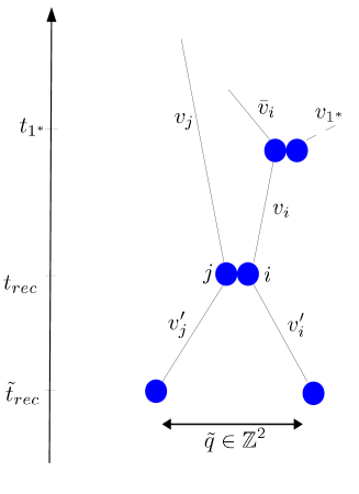
Figure 17. On the left, two recollisions in chain due to periodicity. On the right, the symmetry argument (B.56).

Lemma B.4.

Fix a final configuration of bounded energy $z_{1}\in\mathbb{T}^{2}\times B_{R}$ with $1\leq R^{2}\leq C_{0}|\log{\varepsilon}|$, a time $1\leq t\leq C_{0}|\log{\varepsilon}|$ and a collision tree $a\in\mathcal{A}_{s}$ with $s\geq 2$.

There exists a set of bad parameters $\mathcal{P}_{2}(a,p_{4},\sigma)\subset\mathcal{T}_{2,s}\times{\mathbb{S}}^{s-1}\times\mathbb{R}^{2(s-1)}$ and $\sigma\subset\{2,\dots,s\}$ of cardinal $|\sigma|\leq 3$ such that

• $\mathcal{P}_{2}(a,p_{4},\sigma)$ is parametrized only in terms of $(t_{m},v_{m},\nu_{m})$ for $m\in\sigma$ and $m<\min\sigma$;

  (B.53) $$\int{\bf 1}_{\mathcal{P}_{2}(a,p_{4},\sigma)}\displaystyle\prod_{m\in\sigma}\,\big{|}\big{(}v_{m}-v_{a(m)}(t_{{m}}))\cdot\nu_{{m}}\big{|}dt_{{m}}d\nu_{{m}}dv_{{m}}\leq C(Rt)^{r}s{\varepsilon}\,,$$

  for some constant $r$,

• and any pseudo-trajectory starting from $z_{1}$ at $t$, with total energy bounded by $R^{2}$, and such that the first two recollisions involve the same two particles which recollide twice in chain is parametrized by

  $$(t_{n},\nu_{n},v_{n})_{2\leq n\leq s}\in\bigcup_{\sigma}\mathcal{P}_{2}(a,p_{4},\sigma)\,.$$

Proof.

We recall the equation (3.9) on the first recollision

(B.54) $$v_{i}-v_{j}=\frac{1}{\tau_{rec}}(\delta x_{\perp}-\tau_{1}(\bar{v}_{i}-v_{j})-\nu_{rec})\quad\text{with}\quad\frac{1}{|\tau_{rec}|}\leq{4R\over|\tau_{1}||\bar{v}_{i}-v_{j}|}\,.$$

The equation on the second recollision is

(B.55) $$(v^{\prime}_{i}-v^{\prime}_{j})(\tilde{t}_{rec}-t_{rec})={\varepsilon}\tilde{\nu}_{rec}+{\varepsilon}\nu_{rec}+\tilde{q}$$

for some $\tilde{t}_{rec}\geq 0$, $\tilde{\nu}_{rec}\in{\mathbb{S}}$, and $\tilde{q}\in\mathbb{Z}^{2}\setminus\{0\}$. Note that $\tilde{q}\not=0$ as the second recollision occurs from the periodicity. As usual we fix $\tilde{q}$ and multiply the estimates in the end by $O(R^{2}t^{2})$ to take that into account.

The condition (B.55) implies that the vector $v^{\prime}_{i}-v^{\prime}_{j}$ is located in a cone of axis $\tilde{q}$ and angular sector $2{\varepsilon}$. By definition, we have

(B.56) $$v_{i}^{\prime}-v_{j}^{\prime}=(v_{i}-v_{j})-2(v_{i}-v_{j})\cdot\nu_{rec}\;\nu_{rec},$$

which means that $\nu_{rec}^{\perp}$ is the bisector of $v_{i}-v_{j}$ and $v_{i}^{\prime}-v_{j}^{\prime}$ (see Figure 17).

From (B.54), we deduce that the direction of $v_{i}-v_{j}$ is

$${\delta x_{\perp}-\tau_{1}(\bar{v}_{i}-v_{j})\over|\delta x_{\perp}-\tau_{1}(\bar{v}_{i}-v_{j})|}+O\left({1\over|\tau_{1}(\bar{v}_{i}-v_{j})|}\right)\,.$$

From (B.55), we deduce that the direction of $v^{\prime}_{i}-v^{\prime}_{j}$ is

$${\tilde{q}\over|\tilde{q}|}+O({\varepsilon})\,.$$

Finally we get that $\nu_{rec}^{\perp}$ is known up to an error term which can be bounded by

$$\eta={\varepsilon}+{1\over\sqrt{|\tau_{1}(\bar{v}_{i}-v_{j})|}}\,\cdotp$$

Note that we have introduce the square root as in the proof of Lemma B.3 for integrability purposes of the singularity $|\bar{v}_{i}-v_{j}|$.

Plugging this constraint on $\nu_{rec}$ in (B.54), we get that $v^{\prime}_{i}-v_{j}$ has to belong, for each given $q,\tilde{q}$, to a rectangle $\mathcal{R}$ of axis $\delta x_{\perp}-\tau_{1}(\bar{v}_{i}-v_{j})$ and size $R\times R\frac{\eta}{|\tau_{1}(\bar{v}_{i}-v_{j})|}$. By Lemma C.4, we obtain

$$\int{\bf 1}_{\{v_{i}-v_{j}\in\mathcal{R}\}}\;\big{|}\big{(}v_{1}^{*}-v_{j})\cdot\nu_{1}^{*}\big{)}\big{|}dv_{1}^{*}d\nu_{1}^{*}\leq CR^{3}{{\varepsilon}|\log{\varepsilon}|\over\tau_{1}|\bar{v}_{i}-v_{j}|}+{CR^{3}\over\tau_{1}^{3/2}|\bar{v}_{i}-v_{j}|^{3/2}}\,\cdotp$$

Taking the union of the previous rectangles for the different choices of $q,\tilde{q}$, we define the set $\mathcal{P}_{2}(a,p_{4},\sigma)$ associated with the scenario of two particles recolliding twice in chain due to periodicity. By integration with respect to time, we then get

$$\int{\bf 1}_{\mathcal{P}_{2}(a,p_{4},\sigma)}\;\big{|}\big{(}v_{1}^{*}-v_{j})\cdot\nu_{1}^{*}\big{)}\big{|}dv_{1}^{*}d\nu_{1}^{*}dt_{1}^{*}\leq CR^{3}{{\varepsilon}^{2}|\log{\varepsilon}|^{2}\over|\bar{v}_{i}-v_{j}|}+CR^{3}{{\varepsilon}\over|\bar{v}_{i}-v_{j}|^{3/2}}\,\cdotp$$

We then apply twice Lemma C.2 on two parents of $i,j$ to integrate the singularities at small relative velocities.

Given $\sigma$, there are at most $s$ choices for the pair $(i,j)$ as $\sigma$ determines at least one of the labels. Thus the previous scenario leads to the set $\mathcal{P}_{2}(a,p_{4},\sigma)$ with measure controlled by (B.53). ∎

Appendix C Carleman’s parametrization and scattering estimates

In Sections 3, 6 and Appendix B, we were faced with integrals containing singularities in relative velocities $v_{i}-v_{j}$ and with a multiplicative factor of the type $(v^{*}-\bar{v}_{i})\cdot\nu^{*}$ where $v_{i}$ is recovered from $v^{*}$, $\nu^{*}$ and $\bar{v}_{i}$ through a scattering condition. This appendix is devoted to the proof of “tool-box” lemmas for computing these singular integrals. These lemmas are used many times in this paper.

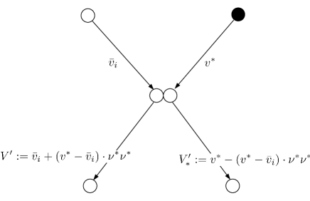
Figure 18. Scattering relations.

Lemma C.1.

Fix a velocity $\bar{v}_{i}$ and let $v_{i},v_{j}$ be the velocities after a collision (with or without scattering)

$$(v_{i},v_{j})=(\bar{v}_{i},v^{*})\quad\text{or}\quad\begin{cases}v_{i}=\bar{v}_{i}+(v^{*}-\bar{v}_{i})\cdot\nu^{*}\nu^{*},\\ v_{j}=v^{*}-(v^{*}-\bar{v}_{i})\cdot\nu^{*}\nu^{*},\end{cases}$$

with $\nu^{*}\in{\mathbb{S}}$ and $v^{*}\in\mathbb{R}^{2}$ (see Figure 18). Assume all the velocities are bounded by $R$ then

(C.1) $$\int{1\over|v_{i}-v_{j}|}\,\big{|}\big{(}v^{*}-\bar{v}_{i})\cdot\nu^{*}\big{|}\,dv^{*}d\nu^{*}\leq CR^{2}.$$

Proof.

In both cases, the velocities before and after the collision are related by $|v_{i}-v_{j}|=|v^{*}-\bar{v}_{i}|$. Inequality (C.1) follows from the fact that the singularity $1/|v^{*}-\bar{v}_{i}|$ is integrable. ∎

Lemma C.2.

Fix $\bar{v}_{i}$ and $v_{j}$, and define $v_{i}$ to be one of the following velocities

(C.2) $$v_{i}=v^{*}-(v^{*}-\bar{v}_{i})\cdot\nu^{*}\nu^{*},$$

$$\mbox{or}\quad v_{i}=\bar{v}_{i}+(v^{*}-\bar{v}_{i})\cdot\nu^{*}\nu^{*}\,,$$

with $\nu^{*}\in{\mathbb{S}}$ and $v^{*}\in B_{R}\subset\mathbb{R}^{2}$ (see Figure 18). Assume all the velocities are bounded by $R>1$ and fix $\delta\in]0,1[$. Then the following estimates hold, denoting $b(\nu^{*},v^{*}):=|(v^{*}-\bar{v}_{i})\cdot\nu^{*}|$:

(C.3) $$\int{\bf 1}_{|v_{i}-v_{j}|\leq\delta}\,b(\nu^{*},v^{*})\,dv^{*}d\nu^{*}\!\!\! \leq \!\!\!CR^{2}\delta\min\left({\delta\over|v_{j}-\bar{v}_{i}|},1\right)\,,$$

(C.4) $$\int\!\!\min\left({\delta\over|v_{i}-v_{j}|},1\right)b(\nu^{*},v^{*})\,dv^{*}d\nu^{*} \leq CR^{2}\delta|\log\delta|{+CR^{3}\delta}\,,$$

(C.5) $$\int{1\over|v_{i}-v_{j}|}\,b(\nu^{*},v^{*})\,dv^{*}d\nu^{*}\!\!\! \leq \!\!\!CR^{2}\Big{(}\big{|}\log|\bar{v}_{i}-v_{j}|\big{|}+R\Big{)}\,,$$

(C.6) $$\int{1\over|v_{i}-v_{j}|^{\gamma}}\,b(\nu^{*},v^{*})\,dv^{*}d\nu^{*}\!\!\! \leq \!\!\!{CR^{2}\over|\bar{v}_{i}-v_{j}|^{\gamma-1}}+CR^{3}\quad\mbox{ for }\,\gamma\in]1,2[\,,$$

(C.7) $$\int{1\over|v_{i}-v_{j}|^{\gamma}}\,b(\nu^{*},v^{*})\,dv^{*}d\nu^{*}\!\!\! \leq \!\!\!CR^{3}\quad\mbox{ for }\,\gamma\in]0,1[\,,$$

(C.8) $$\int\big{|}\log|v_{i}-v_{j}|\big{|}\,b(\nu^{*},v^{*})\,dv^{*}d\nu^{*}\!\!\! \leq \!\!\!CR^{3}\,.$$

Proof.

We start by recalling Carleman’s parametrization, which we shall be using many times in this Appendix: it is defined by

(C.9) $$(v^{*},\nu^{*})\in\mathbb{R}^{2}\times{\mathbb{S}}\mapsto\begin{cases}V^{\prime}_{*}:=v^{*}-(v^{*}-\bar{v}_{i})\cdot\nu^{*}\nu^{*}\\ V^{\prime}:=\bar{v}_{i}+(v^{*}-\bar{v}_{i})\cdot\nu^{*}\nu^{*}\end{cases}$$

where $(V^{\prime},V^{\prime}_{*})$ belong to the set ${\mathcal{C}}$ defined by

$${\mathcal{C}}:=\Big{\{}(V^{\prime},V^{\prime}_{*})\in\mathbb{R}^{2}\times\mathbb{R}^{2}\,/\,(V^{\prime}-\bar{v}_{i})\cdot(V^{\prime}_{*}-\bar{v}_{i})=0\Big{\}}\,.$$

This map sends the measure $b(\nu^{*},v^{*})\,dv^{*}d\nu^{*}$ on the measure $dV^{\prime}dS(V^{\prime}_{*})$, where $dS$ is the Lebesgue measure on the line orthogonal to $(V^{\prime}-\bar{v}_{i})$ passing through $\bar{v}_{i}$.

Now let us consider the case when $|v_{i}-v_{j}|\leq\delta$ and prove (C.3). What we need here is to estimate the measure of the pre-image of the small ball of center $v_{j}$ and radius $\delta$ by the scattering operator: let us study how for fixed $v_{j}$, the set $\{|v_{i}-v_{j}|\leq\delta\}$ is transformed by the inverse scattering map. Notice that the most singular case concerns the case when $v_{i}=V^{\prime}_{*}$ belongs to the small ball of radius $\delta$: indeed in the case when it is $V^{\prime}$ then the measure $b(\nu^{*},v^{*})\,dv^{*}d\nu^{*}$ will have support in a domain of size $O(\delta^{2})$. So now assume that $V^{\prime}_{*}$ satisfies $|V^{\prime}_{*}-v_{j}|\leq\delta$.

Figure 19. $V^{\prime}_{*}$ has to belong to the ball of radius $\delta$ around $v_{j}$, thus it has to be in the cone with the doted lines. By Carleman’s parametrization, this imposes constraints on the angular sector of $V^{\prime}-\bar{v}_{i}$.

$\bullet$ If $|v_{j}-\bar{v}_{i}|\leq\delta$, meaning that $\bar{v}_{i}$ is itself in the same ball, then for any $V^{\prime}\in B_{R}$, the intersection between the small ball and the line $\bar{v}_{i}+\mathbb{R}(V^{\prime}-\bar{v}_{i})^{\perp}$ is a segment, the length of which is at most $\delta$. We therefore find

$$\int{\bf 1}_{|V^{\prime}_{*}-v_{j}|\leq\delta}\,b(\nu^{*},v^{*})\,dv^{*}d\nu^{*}\leq CR^{2}\delta\,.$$

$\bullet$ If $|v_{j}-\bar{v}_{i}|>\delta$, in order for the intersection between the ball and the line $\bar{v}_{i}+\mathbb{R}(V^{\prime}-\bar{v}_{i})^{\perp}$ to be non empty, we have the additional condition that $V^{\prime}-\bar{v}_{i}$ has to be in an angular sector of size $\delta/|v_{j}-\bar{v}_{i}|$ (see Figure 19). We therefore have

$$\int{\bf 1}_{|V^{\prime}_{*}-v_{j}|\leq\delta}\,b(\nu^{*},v^{*})\,dv^{*}d\nu^{*}\leq CR^{2}{\delta^{2}\over|v_{j}-\bar{v}_{i}|}\,\cdotp$$

Thus (C.3) holds.

The other estimates provided in Lemma C.2 then come from Fubini’s theorem: let us start with (C.4). We write

$$\int\min\big{(}{\delta\over|v_{i}-v_{j}|},1\big{)}\,b(\nu^{*},v^{*})\,dv^{*}d\nu^{*} =\int{\bf 1}_{|v_{i}-v_{j}|\leq\delta}\,b(\nu^{*},v^{*})\,dv^{*}d\nu^{*}$$

$$\qquad+\int{\bf 1}_{|v_{i}-v_{j}|>\delta}{\delta\over|v_{i}-v_{j}|}\,b(\nu^{*},v^{*})\,dv^{*}d\nu^{*}$$

$$\leq CR^{2}\delta+\int{\bf 1}_{|v_{i}-v_{j}|>\delta}{\delta\over|v_{i}-v_{j}|}\,b(\nu^{*},v^{*})\,dv^{*}d\nu^{*}$$

thanks to (C.3). The contribution of the velocities such that $|v_{i}-v_{j}|\geq 1$ can be bounded by $R^{3}\delta$. Thus it is enough to consider

$$\int{\delta{\bf 1}_{1\geq|v_{i}-v_{j}|>\delta}\over|v_{i}-v_{j}|}\,b(\nu^{*},v^{*})\,dv^{*}d\nu^{*} =\delta\int\Big{(}\int_{|v_{i}-v_{j}|}^{1}\frac{dr}{r^{2}}+1\Big{)}{\bf 1}_{1\geq|v_{i}-v_{j}|>\delta}\,b(\nu^{*},v^{*})\,dv^{*}d\nu^{*}$$

$$\leq\delta\int_{\delta}^{1}\frac{dr}{r^{2}}\int{\bf 1}_{|v_{i}-v_{j}|\leq r}\,b(\nu^{*},v^{*})\,dv^{*}d\nu^{*}+CR^{3}\delta\,,$$

so using (C.3) again we get

$$\int{\bf 1}_{1\geq|v_{i}-v_{j}|>\delta}{\delta\over|v_{i}-v_{j}|}\,b(\nu^{*},v^{*})\,dv^{*}d\nu^{*} \leq CR^{2}\delta\int_{\delta}^{1}\frac{dr}{r}+CR^{3}\delta\,,$$

from which (C.4) follows.

Next let us prove (C.5)-(C.7). We have

$$\int{1\over|v_{i}-v_{j}|^{\gamma}}\,b(\nu^{*},v^{*})\,dv^{*}d\nu^{*} =\gamma\int\Big{(}\int_{|v_{i}-v_{j}|}^{1}\frac{1}{r^{1+\gamma}}dr+1\Big{)}\,b(\nu^{*},v^{*})\,dv^{*}d\nu^{*}$$

$$=\gamma\int_{0}^{1}\frac{1}{r^{\gamma+1}}\Big{(}\int{\bf 1}_{|v_{i}-v_{j}|\leq r}\,b(\nu^{*},v^{*})\,dv^{*}d\nu^{*}\Big{)}dr+CR^{3}$$

$$\leq C_{\gamma}R^{2}\Big{(}\int_{0}^{|v_{j}-\bar{v}_{i}|}\frac{1}{|v_{j}-\bar{v}_{i}|}r^{1-\gamma}dr+\int_{|v_{j}-\bar{v}_{i}|}^{1}\frac{1}{r^{\gamma}}dr\Big{)}+CR^{3}$$

which gives the expected estimates. Similarly

$$\int\big{|}\log|v_{i}-v_{j}|\big{|}\,b(\nu^{*},v^{*})\,dv^{*}d\nu^{*} =\int\int_{|v_{i}-v_{j}|}^{1}\frac{1}{r}dr\,b(\nu^{*},v^{*})\,dv^{*}d\nu^{*}$$

$$\leq CR^{2}\left(\int_{0}^{|v_{j}-\bar{v}_{i}|}\frac{r}{|v_{j}-\bar{v}_{i}|}dr+\int_{|v_{j}-\bar{v}_{i}|}^{1}dr\right)\leq CR^{3}\,.$$

This ends the proof of Lemma C.2. ∎

Remark C.3.

The proof of Lemma C.2 shows that in order to keep control on the collision integral the power $\gamma$ of the singularity must not be too large (namely smaller than $2$).

Finally the following result describes the size of a collision integral when relative velocities are prescribed to lie in a given rectangle.

Lemma C.4.

Consider two pseudo-particles $i$, $j$ as well as their first parent $1^{*}$. Denote by $\nu_{1^{*}}\in{\mathbb{S}}$ and $v_{1^{*}}\in\mathbb{R}^{2}$ their scattering parameters. We assume also that all the velocities are bounded by $R>1$. Let $\mathcal{R}$ be a rectangle with sides of length $\delta,\delta^{\prime}$, then

(C.10) $$\int{\bf 1}_{v_{i}-v_{j}\in\mathcal{R}}\;\big{|}(v_{1^{*}}-v_{a(1^{*})})\cdot\nu_{1^{*}}\big{|}\,dv_{1^{*}}d\nu_{1^{*}}\leq CR^{2}\min(\delta,\delta^{\prime})\big{(}|\log\delta|+|\log\delta^{\prime}|+1\big{)},$$

Proof.

Note that if $i,j$ are generated by the same collision, then better estimates can be obtained from Lemma C.1. The case without scattering is also straightforward. Thus from now, we assume that $v_{i}$ is given by (C.2).

To derive (C.10), we suppose that $\delta\leq\delta^{\prime}\leq 1$ and that the collision with $1^{*}$ takes place with $i$ which had a velocity $\bar{v}_{i}$. We cover the rectangle $v_{j}+\mathcal{R}$ into $\lfloor\delta^{\prime}/\delta\rfloor$ balls of radius $2\delta$. Let $\omega$ be the axis of the rectangle $v_{j}+\mathcal{R}$ and denote by $w_{k}=w_{0}+\delta k\,\omega$ the centers of the balls which are indexed by the integer $k\in\{0,\dots,\lfloor\delta^{\prime}/\delta\rfloor\}$. Applying (C.3) to each ball, we get

$$\int{\bf 1}_{v_{i}-v_{j}\in\mathcal{R}}\;b(\nu_{1^{*}},v_{1^{*}})\,dv_{1^{*}}d\nu_{1^{*}} \leq \sum_{k=0}^{\lfloor\delta^{\prime}/\delta\rfloor}\int{\bf 1}_{|v_{i}-w_{k}|\leq 2\delta}\;b(\nu_{1^{*}},v_{1^{*}})\,dv_{1^{*}}d\nu_{1^{*}}$$

$$\leq CR^{2}\sum_{k=0}^{\lfloor\delta^{\prime}/\delta\rfloor}\delta\min\left({\delta\over|w_{k}-\bar{v}_{i}|},1\right),$$

$$\leq CR^{2}\delta\sum_{k=0}^{\lfloor\delta^{\prime}/\delta\rfloor}{\delta\over|w_{k}-\bar{v}_{i}|+\delta}\leq CR^{2}\delta\left(\log(\frac{\delta^{\prime}}{\delta})+1\right),$$

where the log divergence in the last inequality follows by summing over $k$. This completes the proof of (C.10).

This completes the proof of Lemma C.4. ∎

Appendix D Initial data estimates

This section is devoted to the proof of Proposition 2.6 stated page 2.6.

Using the notation $X_{k,N}:=\{x_{k},\dots,x_{N}\}$, we write

$$\Big{|}\left(f_{N}^{0(s)}-f^{(s)}_{0}\right)(Z_{s}){\bf 1}_{{\mathcal{D}}_{{\varepsilon}}^{s}}(X_{s})\Big{|}\leq M_{\beta}^{\otimes s}(V_{s})\sum_{i=1}^{s}\big{|}g_{\alpha,0}(z_{i})\big{|}\,\Big{|}{\mathcal{Z}}_{N}^{-1}\int{\bf 1}_{{\mathcal{D}}_{{\varepsilon}}^{N}}(X_{N})\,dX_{s+1,N}-1\Big{|}$$

$$+{}{\mathcal{Z}}_{N}^{-1}M_{\beta}^{\otimes s}(V_{s})\sum_{i=s+1}^{N}\Big{|}\int M_{\beta}(v_{i})g_{\alpha,0}(z_{i}){\bf 1}_{{\mathcal{D}}_{{\varepsilon}}^{N}}(X_{N})\,dv_{i}dX_{s+1,N}\Big{|}\,,$$

where ${\mathcal{D}}_{{\varepsilon}}^{N}$ stands for the exclusion constraint on the positions (with a slight abuse of notation compared to (1.4)). The first term is estimated as in the proof of Proposition 3.3 in [9]

$$M_{\beta}^{\otimes s}(V_{s})\sum_{i=1}^{s}\big{|}g_{\alpha,0}(z_{i})\big{|}\,\Big{|}{\mathcal{Z}}_{N}^{-1}\int{\bf 1}_{{\mathcal{D}}_{{\varepsilon}}^{N}}(X_{N})\,dX_{s+1,N}-1\Big{|}\leq C^{s}{\varepsilon}\alpha M_{\beta}^{\otimes s}(V_{s})\|g_{\alpha,0}\|_{L^{\infty}}\,.$$

The exchangeability of the variables allows us to rewrite the second term as

$$I(Z_{s}) :={\mathcal{Z}}_{N}^{-1}M_{\beta}^{\otimes s}(V_{s})\sum_{i=s+1}^{N}\Big{|}\int M_{\beta}(v_{i})g_{\alpha,0}(z_{i}){\bf 1}_{{\mathcal{D}}_{{\varepsilon}}^{N}}(X_{N})\,dv_{i}dX_{s+1,N}\Big{|}$$

$$\,\leq(N-s)M_{\beta}^{\otimes s}(V_{s}){\mathcal{Z}}_{N}^{-1}$$

$$\qquad\qquad\Big{|}\int M_{\beta}(v_{s+1})g_{\alpha,0}(z_{s+1})\Big{(}\prod_{k\neq s+1}{\bf 1}_{|x_{k}-x_{s+1}|>{\varepsilon}}\Big{)}\;\chi_{s+2}(X_{N})\,dz_{s+1}dX_{s+2,N}\Big{|}\,,$$

where we used the notation

(D.1) $$\chi_{s+2}(X_{N}):=\hat{\chi}^{+}_{s+2}(X_{s+2,N})\,\hat{\chi}^{-}_{s+2}(X_{N})$$

which distinguishes the interaction of the particles $X_{s+2,N}$ with themselves and with $X_{s}$, defining

$$\hat{\chi}^{+}_{s+2}(X_{s+2,N}):=\prod_{s+2\leq\ell<k\leq N}{\bf 1}_{|x_{k}-x_{\ell}|>{\varepsilon}}\quad\text{and}\quad\hat{\chi}^{-}_{s+2}(X_{N}):=\prod_{s+2\leq\ell\leq N\atop 1\leq k\leq s}{\bf 1}_{|x_{k}-x_{\ell}|>{\varepsilon}}\,.$$

The exclusion between $s+1$ and the rest of the system is also decomposed into a term for the interaction with $X_{s}$ and another one for the interaction with $X_{s+2,N}$. Defining

$$\chi^{-}_{s+1}(X_{s+1}):=\prod_{k\leq s}{\bf 1}_{|x_{k}-x_{s+1}|>{\varepsilon}}\quad\text{and}\quad\chi^{+}_{s+1}(X_{s+1,N}):=\prod_{k\geq s+2}{\bf 1}_{|x_{k}-x_{s+1}|>{\varepsilon}}$$

we have

$$\prod_{k\neq s+1}{\bf 1}_{|x_{k}-x_{s+1}|>{\varepsilon}} =\chi^{-}_{s+1}(X_{s+1})\,\chi^{+}_{s+1}(X_{s+1,N})$$

$$=\chi^{+}_{s+1}(X_{s+1,N})-\big{(}1-\chi^{-}_{s+1}(X_{s+1})\big{)}\chi^{+}_{s+1}(X_{s+1,N})\,.$$

We deduce that

$$I(Z_{s})\leq M_{\beta}^{\otimes s}(V_{s})\Big{(}I_{1}(Z_{s})+I_{2}(Z_{s})\Big{)}$$

with

$$\begin{cases}\displaystyle I_{1}(Z_{s}):={\mathcal{Z}}_{N}^{-1}N\int M_{\beta}(v_{s+1})\big{|}g_{\alpha,0}(z_{s+1})\big{|}\big{(}1-\chi^{-}_{s+1}(X_{s+1})\big{)}\hat{\chi}^{+}_{s+2}(X_{s+2,N})\,dz_{s+1}dX_{s+2,N}\,,\\ \displaystyle I_{2}(Z_{s}):={\mathcal{Z}}_{N}^{-1}N\Big{|}\int M_{\beta}(v_{s+1})g_{\alpha,0}(z_{s+1})\chi^{+}_{s+1}(X_{s+2,N})\;\chi_{s+2}(X_{N})\,dz_{s+1}dX_{s+2,N}\Big{|}\,.\end{cases}$$

From (2.14) and the assumption $N{\varepsilon}=\alpha\ll 1/{\varepsilon}$, we get

$${\mathcal{Z}}_{N}^{-1}\int\hat{\chi}^{+}_{s+2}(X_{s+2,N})\,dX_{s+2,N}=\frac{{\mathcal{Z}}_{N-s-2}}{{\mathcal{Z}}_{N}}\leq\exp\big{(}Cs\alpha{\varepsilon}\big{)}\leq\exp\big{(}Cs\big{)}\,.$$

We infer that the term $I_{1}$ is bounded by the fact that $x_{s+1}$ is close to $X_{s}$

$$I_{1}(Z_{s})\leq sN{\varepsilon}^{2}\exp\big{(}Cs\big{)}\|g_{\alpha,0}\|_{L^{\infty}}\leq s\exp\big{(}Cs\big{)}\alpha{\varepsilon}\|g_{\alpha,0}\|_{L^{\infty}}\,.$$

Using the assumption $\displaystyle\int_{\mathbb{D}}M_{\beta}g_{\alpha,0}(z)dz=0$, the second term is rewritten as

$$I_{2}(Z_{s})={\mathcal{Z}}_{N}^{-1}N\big{|}\int M_{\beta}(v_{s+1})g_{\alpha,0}(z_{s+1})\big{(}1-\chi^{+}_{s+1}(X_{s+1,N})\big{)}\;\chi_{s+2}(X_{N})\,dz_{s+1}dX_{s+2,N}\big{|}\,.$$

Plugging the identity (D.1)

$$\chi_{s+2}(X_{N})=\hat{\chi}^{+}_{s+2}(X_{s+2,N})-\big{(}1-\hat{\chi}^{-}_{s+2}(X_{N})\big{)}\hat{\chi}^{+}_{s+2}(X_{s+2,N})$$

we distinguish two more contributions $I_{2}(Z_{s})\leq I_{2,1}(Z_{s})+I_{2,2}(Z_{s})$ with

$$\begin{cases}\displaystyle I_{2,1}(Z_{s}):={\mathcal{Z}}_{N}^{-1}N\|g_{\alpha,0}\|_{L^{\infty}}\,\int\big{(}1-\chi^{+}_{s+1}(X_{s+1,N})\big{)}\;\big{(}1-\hat{\chi}^{-}_{s+2}(X_{N})\big{)}\hat{\chi}^{+}_{s+2}(X_{s+2,N})\,dX_{s+1,N}\,,\\ \displaystyle I_{2,2}(Z_{s}):={\mathcal{Z}}_{N}^{-1}N\Big{|}\int M_{\beta}(v_{s+1})g_{\alpha,0}(z_{s+1})\big{(}1-\chi^{+}_{s+1}(X_{s+1,N})\big{)}\;\hat{\chi}^{+}_{s+2}(X_{s+2,N})\,dz_{s+1}dX_{s+2,N}\Big{|}\,.\\ \end{cases}$$

The term $I_{2,1}$ takes into account two constraints : $s+1$ is close to a particle in $X_{s+2,N}$ and one particle in $X_{s+2,N}$ is close to $X_{s}$. Since $N{\varepsilon}=\alpha$, we deduce that

$$I_{2,1}(Z_{s})\leq Ns{\varepsilon}^{2}\,(N-s-1)^{2}{\varepsilon}^{2}\,\frac{{\mathcal{Z}}_{N-s-3}}{{\mathcal{Z}}_{N}}\|g_{\alpha,0}\|_{L^{\infty}}\leq s\alpha^{3}{\varepsilon}\exp(Cs)\|g_{\alpha,0}\|_{L^{\infty}}\,.$$

The term $I_{2,2}$ does not depend on $X_{s}$, thus one can integrate over $z_{s+1}$ and use again the assumption $\displaystyle\int_{\mathbb{D}}M_{\beta}g_{\alpha,0}(z)dz=0$. To see this, it is enough to note that the function

$$x_{s+1}\mapsto\int\big{(}1-\chi^{+}_{s+1}(X_{s+1,N})\big{)}\;\hat{\chi}^{+}_{s+2}(X_{s+2,N})dX_{s+2,N}$$

is independent of $x_{s+1}$ thanks to the periodic structure of $\mathbb{D}^{N-s-2}$. Thus $I_{2,2}(Z_{s})=0$.

Combining the previous estimates, we conclude Proposition 2.6. ∎

References

- [1] R. Alexander, The Infinite Hard Sphere System, Ph.D. dissertation, Dept. Mathematics, Univ. California, Berkeley, 1975.
- [2] N. Ayi, From Newton’s law to the linear Boltzmann equation without cut-off, accepted for publication, Comm. Math. Phys.
- [3] C. Bardos, F. Golse, C.D. Levermore, Fluid Dynamic Limits of Kinetic Equations II: Convergence Proofs for the Boltzmann Equation, Comm. Pure & Appl. Math 46 (1993), 667–753.
- [4] H. van Beijeren, O.E. Lanford, J. Lebowitz, H. Spohn, Equilibrium time correlation functions in the low-density limit, J. Statist. Phys. 22 (1980), 2, 237–257.
- [5] T. Bodineau, I. Gallagher, L. Saint-Raymond, The Brownian motion as the limit of a deterministic system of hard-spheres, Inventiones (2015), 1–61.
- [6] R.E. Caflisch: The fluid dynamic limit of the nonlinear Boltzmann equation, Comm. on Pure and Appl. Math. 33 (1980), 651–666.
- [7] C. Cercignani, R. Illner, M. Pulvirenti, The Mathematical Theory of Dilute Gases, Springer Verlag, New York NY, 1994.
- [8] R. DiPerna, P.-L. Lions, On the Cauchy problem for Boltzmann equations: global existence and weak stability, Ann. of Math. (2) 130 (1989), no. 2, p. 321-366.
- [9] I. Gallagher, L. Saint-Raymond, B. Texier, From Newton to Boltzmann : the case of hard-spheres and short-range potentials, ZLAM (2014).
- [10] F. Golse, D. Levermore, The Stokes-Fourier and Acoustic Limits for the Boltzmann Equation, Comm. on Pure and Appl. Math. 55 (2002), 336–393.
- [11] F. Golse, L. Saint-Raymond, The Incompressible Navier-Stokes Limit of the Boltzmann Equation for Hard Cutoff Potentials, J. Math. Pures Appl. 91 (2009), 508–552.
- [12] H. Grad, Principles of the kinetic theory of gases, Handbuch der Physik 12, Thermodynamik der Gase p. 205-294 Springer-Verlag, Berlin-Gottingen-Heidelberg, 1958.
- [13] Y. Guo, The Boltzmann equation in the whole space, Indiana Univ. Math. J. 53 (2004), 1081–1094.
- [14] E. Hewitt, L. Savage, Symmetric measures on Cartesian products. Trans. Amer. Math. Soc. 80 (1955), 470-501.
- [15] D. Hilbert, Mathematical problems Bull. Amer. Math. Soc. 8 (1902), no. 10, 437–479.
- [16] D. Hilbert, Begründung der kinetischen Gastheorie Math. Ann. 72 (1912), 562–577.
- [17] F. King, BBGKY hierarchy for positive potentials, Ph.D. dissertation, Dept. Mathematics, Univ. California, Berkeley, 1975.
- [18] O.E. Lanford, Time evolution of large classical systems, Lect. Notes in Physics 38, J. Moser ed., 1–111, Springer Verlag (1975).
- [19] J. L. Lebowitz, J. K. Percus, J. Sykes, Time evolution of the total distribution function of a one-dimensional system of hard rods, Physical Review 171 (1968), (1), 224.
- [20] T.-P. Liu, S.-H. Yu : Boltzmann equation: micro-macro decompositions and positivity of shock profiles, Comm. Math. Phys. 246 (2004), 133–179.
- [21] B. Perthame: Introduction to the collision models in Boltzmann’s theory, in “Modeling of Collisions”, P.-A. Raviart ed., Masson, Paris, 1997.
- [22] M. Pulvirenti, C. Saffirio, S. Simonella, On the validity of the Boltzmann equation for short range potentials, Reviews in Mathematical Physics, 26 (2014), (2), 1450001.
- [23] M. Pulvirenti, S. Simonella, The Boltzmann-Grad limit of a hard sphere system: analysis of the correlation error, Invent. math. (2016). doi:10.1007/s00222-016-0682-4
- [24] F. Rezakhanlou, Equilibrium fluctuations for the discrete Boltzmann equation, Duke mathematical journal, 93 (1998), (2), 257-288.
- [25] S. Simonella, Evolution of correlation functions in the hard sphere dynamics, Journal of Statistical Physics, 155 (2014), (6), 1191-1221.
- [26] H. Spohn, Boltzmann hierarchy and Boltzmann equation, in Kinetic theories and the Boltzmann equation (Montecatini, 1981), 207-220.
- [27] H. Spohn, Large scale dynamics of interacting particles, Springer-Verlag 174 (1991).
- [28] H. Spohn, Fluctuations around the Boltzman equation, Journal of Statistical Physics, 26 (1981), (2), 285-305.
- [29] K. Uchiyama, Derivation of the Boltzmann equation from particle dynamics, Hiroshima Math. J. 18 (1988), (2), 245-297.
- [30] S. Ukai. On the existence of global solutions of a mixed problem for the nonlinear Boltzman equation, Proc. of the Japan Acad. 50 (1974), 179-184.