Learning with a Strong Adversary

Abstract

The robustness of neural networks to intended perturbations has recently attracted significant attention. In this paper, we propose a new method, learning with a strong adversary, that learns robust classifiers from supervised data by generating adversarial examples as an intermediate step. A new and simple way of finding adversarial examples is presented that is empirically stronger than existing approaches in terms of the accuracy reduction as a function of perturbation magnitude. Experimental results demonstrate that resulting learning method greatly improves the robustness of the classification models produced.

1 Introduction

Deep Neural Network (DNN) models have recently demonstrated impressive learning results in many visual and speech classification problems (Krizhevsky et al., 2012; Hinton et al., 2012a). One reason for this success is believed to be the expressive capacity of deep network architectures. Even though classifiers are typically evaluated by their misclassification rate, robustness is also a highly desirable property: intuitively, it is desirable for a classifier to be ‘smooth’ in the sense that a small perturbation of its input should not change its predictions significantly. An intriguing recent discovery is that DNN models do not typically possess such a robustness property (Szegedy et al., 2013). An otherwise highly accurate DNN model can be fooled into misclassifying typical data points by introducing a human-indistinguishable perturbation of the original inputs. We call such a perturbed data set ‘adversarial examples’. An even more curious fact is that the same set of such adversarial examples is also misclassified by a diverse set of classification models, such as KNN, Boosting Tree, even if they are trained with different architectures and different hyperparameters.

Since the appearance of Szegedy et al. (2013), increasing attention has been paid to the curious phenomenon of ‘adversarial perturbation’ in the deep learning community; see, for example (Goodfellow et al., 2014; Fawzi et al., 2015; Miyato et al., 2015; Nøkland, 2015; Tabacof & Valle, 2015). Goodfellow et al. (2014) suggest that one reason for the detrimental effect of adversarial examples lies in the implicit linearity of the classification models in high dimensional spaces. Additional exploration by Tabacof & Valle (2015) has demonstrated that, for image classification problems, adversarial images inhabit large ”adversarial pockets” in the pixel space. Based on these observations, different ways of finding adversarial examples have been proposed, among which the most relevant to our study is that of (Goodfellow et al., 2014), where a linear approximation is used to obviate the need for any auxiliary optimization problem to be solved. In this paper, we further investigate the role of adversarial training on classifier robustness and propose a simple new approach to finding ’stronger’ adversarial examples. Experimental results suggest that the proposed method is more effective than previous approaches in the sense that the resulting DNN classifiers obtain worse performance under the same magnitude of perturbation.

The main achievement of this paper is a training method that is able to produce robust classifiers with high classification accuracy in the face of stronger data perturbation. The approach we propose differs from previous approaches in a few ways. First, Goodfellow et al. (2014) suggests using an augmented objective that combines the original training objective with an additional objective that is measured after after the training inputs have been perturbed. Alternatively, (Nøkland, 2015) suggest, as a specialization of the method in (Goodfellow et al., 2014), to only use the objective defined on the perturbed data. However, there is no theoretical analysis to justify that classifiers learned in this way are indeed robust; both methods are proposed heuristically. In our proposed approach, we formulate the learning procedure as a min-max problem that forces the learned DNN model to be robust against adversarial examples, so that the learned classifier is inherently robust. In particular, we allow an adversary to apply perturbations to each data point in an attempt to maximize classification error, while the learning procedure attempts to minimize misclassification error against the adversary. We call this learning procedure ‘learning with a strong adversary’. Such min-max formulation has been discussed specifically in (Goodfellow et al., 2014), but emphasis is on its regularization effect particularly for logistic regression. Our setting is more general and applicable to different loss functions and different types of perturbations, and is the origin of our learning procedure. It turns out that an efficient method for finding such adversarial examples is required as an intermediate step to solve such a min-max problem, which is the first problem we address. Then we develop the full min-max training procedure that incorporates robustness to adversarially perturbed training data. The learning procedure that results turns out to have some similarities to the one proposed in (Nøkland, 2015). Another min-max formulation is proposed in Miyato et al. (2015) but still with the interpretation of regularization. These approaches are based on significantly different understandings of this problem. Recently, a theoretical exploration of the robustness of classifiers (Fawzi et al., 2015) suggests that, as expected, there is a trade-off between expressive power and robustness. This paper can be considered as an exploration into this same trade-off from an engineering perspective.

The remainder of the paper is organized as follows. First, we propose a new method for finding adversarial examples in Section 2. Section 3 is then devoted to developing the main method: a new procedure for learning with a stronger form of adversary. Finally, we provide an experimental evaluation of the proposed method on MNIST and CIFAR-10 in Section 4.

1.1 Notations

We denote the supervised training data by $\underline{Z}=\{(x_{1},y_{1}),\ldots,(x_{N},y_{N})\}$. Let $K$ be the number of classes in the classification problem. The loss function used for training will be denoted by $\ell$. Given a norm $\|\cdot\|$, let $\|\cdot\|_{*}$ denote its dual norm, such that $\|u\|_{*}=\max_{\|v\|\leq 1}\langle u,\,v\rangle$. Denote the network by $\mathcal{N}$ whose last layer is a softmax layer $g(x)\triangleq\alpha=(\alpha_{1},\ldots,\alpha_{K})$ to be used for classification. So $\mathcal{N}(x)$ is the predicted label for the sample $x$.

2 Finding adversarial examples

Consider an example $(x,y)\in\mathcal{X}\times\{1,2,\ldots,K\}$ and assume that $\mathcal{N}(x)=y$, where $y$ is the true label for $x$. Our goal is to find a small perturbation $r\in\mathcal{X}$ so that $\mathcal{N}(X+r)\neq y$. This problem was originally investigated by Szegedy et al. (2013), who propose the following perturbation procedure: given $x$, solve

$$\min_{r}\|r\|\quad s.t.\quad\mathcal{N}(X+r)\neq\mathcal{N}(X).$$

The simple method we propose to find such a perturbation $r$ is based on the linear approximation of $g(x)$, $\hat{g}(x+r)=g(x)+Hr$, where $H=\frac{\partial g}{\partial w}|_{x}$ is the Jacobian matrix.

As an alternative, we consider the following question: for a fixed index $j\neq y$, what is the minimal $r_{(j)}$ satisfying $\mathcal{N}(x+r_{(j)})=j$? Replacing $g$ by its linear approximation $\hat{g}$, one of the necessary conditions for such a perturbation $r$ is:

$$H_{j}r_{(j)}-H_{y}r_{(j)}\geq\alpha_{y}-\alpha_{j},$$

where $H_{j}$ is the $j$-th row of $H$. Therefore, the norm of the optimal $r_{(j)}^{*}$ is greater than the following objective value:

$$\min_{r_{(j)}}\|r_{(j)}\|\quad s.t.\quad H_{j}r_{(j)}-H_{y}r_{(j)}\geq\alpha_{y}-\alpha_{j}.$$ (1)

The optimal solution to this problem is provided in Proposition 1.

Proposition 1.

It is straightforward that the optimal objective value is $\|r_{(j)}\|=\frac{\alpha_{y}-\alpha_{j}}{\|H_{j}-H_{y}\|_{*}}$. In particular, the optimal $r_{(j)}^{*}$ for common norms are:

1. If $\|\cdot\|$ is the $L_{2}$ norm, then $r_{(j)}^{*}=\frac{\alpha_{y}-\alpha_{j}}{\|H_{j}-H_{y}\|_{2}^{2}}(H_{j}-H_{y})$;

2. If $\|\cdot\|$ is the $L_{\infty}$ norm, then $r_{(j)}^{*}=\frac{\alpha_{y}-\alpha_{j}}{\|H_{j}-H_{y}\|_{1}}\text{sign}(H_{j}-H_{y})$;

3. If $\|\cdot\|$ is the $L_{1}$ norm, then $r_{(j)}^{*}=\frac{c}{\|H_{j}-H_{y}\|_{\infty}}e_{k}$ where $k$ satisfies $|(H_{j}-H_{y})_{k}|=\|H_{j}-H_{y}\|_{\infty}$. Here $V_{k}$ is the $k$-th element of $V$.

However, such $r_{(j)}^{*}$ is necessary but not sufficient to guarantee that $\arg\!\max_{i}\hat{g}(x+r_{(j)})_{i}=j$. The following proposition shows that in order to have $\hat{g}$ make a wrong prediction, it is enough to use the minimum among all $r_{(j)}^{*}$’s.

Proposition 2.

Let $I=\arg\!\min_{i}\|r_{(i)}^{*}\|$. Then $r_{I}^{*}$ is the solution of the following problem:

$$\min_{r}\,\|r\|\quad s.t.\quad\arg\!\max_{i}\,\left(\hat{g}(X+r)\right)_{i}\neq y.$$

Putting these observations together, we achieve an algorithm for finding adversarial examples, as shown in Algorithm 1.

Algorithm 1 Finding Adversarial Examples

0:  $(x,y)$; Network $\mathcal{N}$;

0:  $r$

1:  Compute $H$ by performing forward-backward propagation from the input layer to the softmax layer $g(x)$

2:  for $j=1,2,\ldots,K$ do

3:     Compute $r_{(j)}^{*}$ from Equation (1)

4:  end for

5:  Return $r=r_{(I)}^{*}$ where $I=\arg\!\min_{i}\|r_{(i)}^{*}\|$.

3 Toward Robust Neural Networks

We enhance the robustness of a neural network model by preparing the network for the worst examples by training with the following objective:

$$\min_{g}\sum_{i}\max_{\|r^{(i)}\|\leq c}\ell(g(x_{i}+r^{(i)}),y_{i});$$ (2)

where $g$ ranges over functions expressible by the network model $\mathcal{N}$ (i.e. ranging over all parameters in $\mathcal{N}$). In this formulation, the hyperparameter $c$ that controls the magnitude of the perturbation needs to be tuned. Note that when $\ell(g(x_{i}+r^{(i)}),y_{i})=\mathbb{I}_{(\max_{j}(g(x_{i}+r^{(i)})_{j})\neq y_{i})}$, the objective function is the misclassification error under perturbations. Often, $\ell$ is a surrogate for the misclassification loss that is differentiable and smooth. Let $L_{i}(g)=\max_{\|r^{(i)}\|_{2}\leq c}\ell(g(x_{i}+r^{(i)}),y_{i})$. Thus the problem is to find $g^{*}=\arg\min_{g}\sum_{i}L_{i}(g)$.

Related Works:
1. When taking $\ell$ to be the logistic loss, $g$ to be a linear function, and the norm for perturbation to be $\ell_{\infty}$, then the inner max problem has analytical solution, and Equation (2) matches the learning objective in Section 5 of (Goodfellow et al., 2014).
2. Let $\ell$ be the negative log function and $g$ be the probability predicted by the model. Viewing $y_{i}$ as a distribution that has weight 1 on $y_{i}$ and $0$ on other classes, then the classical entropy loss is in fact $D_{KL}(y_{i}\|p)$ where $p=g(x_{i})$. Using these notions, Equation (2) can be rewritten as $\min_{f}\sum\max_{r^{(i)}}D_{KL}(y_{i}\,\|\tilde{p})$ where $\tilde{p}=g(x_{i}+r^{(i)})$. Similarly, the objective function proposed in (Goodfellow et al., 2014) can be generalized as $\alpha D_{KL}(y_{i}\|p)+(1-\alpha)\max_{r^{(i)}}D_{KL}(y_{i}\|\tilde{p})$. Moreover, the one proposed in Miyato et al. (2015) can be interpreated as $D_{KL}(y_{i}\|p)+D_{KL}(p\|\tilde{p})$. Experiments shows that our approach is able to achieve the best robustness while maintain high classification accuracy.

To solve the problem (2) using SGD, one needs to compute the derivative of $L_{i}$ with respect to (the parameters that define) $g$. The following preliminary proposition suggests a way of computing this derivative.

Proposition 3.

Given $h:\mathcal{U}\times\mathcal{V}\rightarrow\mathcal{W}$ differentiable almost everywhere, define $L(v)=\max_{u\in\mathcal{U}}h(u,v)$. Assume that $L$ is uniformly Lipschitz-continuous as a function of $v$, then the following results holds almost everywhere:

$$\frac{\partial L}{\partial v}(v_{0})=\frac{\partial h}{\partial v}(u^{*},v_{0}),$$

where $u^{*}=\arg\max_{u}h(u,v_{0})$.

Proof.

Note that $L$ is uniformly Lipschitz-continuous, therefore by Rademacher’s theorem, $L$ is differentiable almost everywhere. For $v_{0}$ where $L$ is differentiable, the Fréchet subderivative of $L$ is actually a singleton set of its derivative.

Consider the function $\hat{L}(v)=h(u^{*},v)$. Since $h$ is differentiable, $\frac{\partial h}{\partial v}(u^{*},v_{0})$ is the derivative of $\hat{L}$ at point $v_{0}$. Also $\hat{L}(v_{0})=L(v_{0})$. Thus, by Proposition 2 of (Neu & Szepesvári, 2012), $\frac{\partial h}{\partial v}(u^{*},v_{0})$ also belongs to the subderivative of $L$. Therefore,

$$\frac{\partial L}{\partial v}(v_{0})=\frac{\partial h}{\partial v}(u^{*},v_{0}).$$

∎

The differentiability of $h$ in Proposition 3 usually holds. The uniformly Lipschitz-continuous of neural networks was also discussed in the paper of Szegedy et al. (2013). It still remains to compute $u^{*}$ in Proposition 3. In particular given $(x_{i},y_{i})$, we need to solve

$$\max_{\|r^{(i)}\|\leq c}\ell(g(x_{i}+r^{(i)}),y_{i}).$$ (3)

We postpone the solution for the above problem to the end of this section. Given that we can have an approximate solution for Equation (3), a simple SGD method to compute a local solution for Equation (2) is then shown in Algorithm 2.

Algorithm 2 Learning with an Adversary

0:  $(x_{i},y_{i})$ for $1\leq i\leq N$; Initial $g_{0}$;

0:  $\hat{g}$

1:  for  $t=1,2,\ldots,T$ do

2:     for $(x_{i},y_{i})$ in the current batch do

3:        Use forward-backward propagation to compute $\frac{\partial g}{\partial x}$

4:        Compute $r^{*}$ as the optimal perturbation to $x$, using the proposed methods in Section 3.1

5:        Create a pseudo-sample to be $(\hat{x}_{i}=x_{i}+c\frac{r^{*}}{\|r^{*}\|_{2}},y_{i})$

6:     end for

7:     Update the network $\hat{g}$ using forward-backward propagation on the pseudo-sample $(\hat{x}_{i},y_{i})$ for $1\leq i\leq N$

8:  end for

9:  Return $\hat{g}$.

For complex prediction problems, deeper neural networks are usually proposed, which can be interpreted as consisting of two parts: the lower layers of the network can be interpreted as learning a representation for the input data, while the upper layers can be interpreted as learning a classification model on top of the learned representation. The number of layers that should be interpreted as providing representations versus classifications is not precise and varies between datasets; we treat this as a hyperparameter in our method. Given such an interpretation, denote the representation layers of the network as $\mathcal{N}_{\rm rep}$ and the classification layers of the network as $\mathcal{N}_{\rm cla}$. We propose to perform the perturbation over the output of $\mathcal{N}_{\rm rep}$ rather than the raw data. Thus the problem of learning with an adversary can be formulated as follows:

$$\min_{\mathcal{N}_{\rm rep},\mathcal{N}_{\rm cla}}\sum_{i}\max_{\|r^{(i)}\|\leq c}\ell\left(\mathcal{N}_{\rm cla}\left(\mathcal{N}_{\rm rep}(x_{i})+r^{(i)}\right),y_{i}\right).$$ (4)

Similarly, Equation (4) can be solved by the following SGD method given in Algorithm 3.

Algorithm 3 Learning with an Adversary in the Split Network Interpretation

0:  $(x_{i},y_{i})$ for $1\leq i\leq N$; Initial $\mathcal{N}_{\rm cla}$ and $\mathcal{N}_{\rm rep}$;

0:  $\hat{f}$

1:  for  $t=1,2,\ldots,T$ do

2:     for $(x_{i},y_{i})$ in the current batch do

3:        Use forward propagation to compute the output of $\mathcal{N}_{\rm rep}$, $\tilde{x}_{i}$

4:        Take $\tilde{x}_{i}$ as the input for $\mathcal{N}_{\rm cla}$

5:        Use forward-backward propagation to compute $\frac{\partial\alpha}{\partial\tilde{x}_{i}}$

6:        Compute $r^{*}$ as the optimal perturbation to $\tilde{x}_{i}$, using the proposed methods in Section 3.1

7:        Create a pseudo-sample to be $(\hat{\tilde{x}}_{i}=\tilde{x}_{i}+c\frac{r^{*}}{\|r^{*}\|},y_{i})$

8:     end for

9:     Use forward propagation to compute the output of $\mathcal{N}_{\rm cla}$ on $(\hat{\tilde{x}}_{i},y_{i})$ for $1\leq i\leq N$

10:     Use backward propagation to update both $\mathcal{N}_{\rm cla}$

11:     Use backward propagation to compute $\frac{\partial\mathcal{N}_{\rm rep}}{\partial W}|_{\tilde{x_{i}},y_{i}}$

12:     Update $\mathcal{N}_{\rm rep}$ by $\frac{\partial\ell}{\partial\tilde{x}_{i}}|_{(\hat{\tilde{x}}_{i},y_{i})}\frac{\partial\mathcal{N}_{\rm rep}}{\partial W}|_{\tilde{x_{i}},y_{i}}$

13:  end for

14:  Return $\mathcal{N}_{\rm cla}$ and $\mathcal{N}_{\rm rep}$

3.1 Computing the perturbation

We propose two different perturbation methods based on two different principles. The first proposed method, similar to that of (Goodfellow et al., 2014), does not require the solution of an optimization problem. Experimental results show that this method, compared to the method proposed in (Goodfellow et al., 2014), is more effective in the sense that, under the same magnitude of perturbation, the accuracy reduction in the network is greater.

3.1.1 Likelihood Based Loss

Assume the loss function $\ell(x,y)=h(\alpha_{y})$, where $h$ is a non-negative decreasing function. A typical example of such a loss would be the logistic regression loss. In fact, most of the network models use a softmax layer as the last layer and a cross-entropy objective function. Recall that we would like to find

$$r^{*}=\arg\max_{\|r^{(i)}\|\leq c}h\left(g(x_{i}+r^{(i)})_{y_{i}}\right),$$ (5)

where $x_{i}$ could be the raw data or the output of $\mathcal{N}_{\rm rep}$. Since $h$ is decreasing, $r^{*}=\arg\min_{\|r^{(i)}\|\leq c}g(x_{i}+r^{(i)})_{y_{i}}$.

This problem can still be difficult to solve in general. Similarly, using its linear approximation $\tilde{g}(x_{i}+r^{(i)})_{y_{i}}$, i.e. $g(x_{i}+r^{(i)})_{y_{i}}\approx\tilde{g}(x_{i}+r^{(i)})_{y_{i}}=g(x_{i})_{y_{i}}+\langle H_{y_{i}},\,r^{(i)}\rangle$, such that $H=\frac{\partial g}{\partial w}|_{x}$ is the Jacobian matrix, it is then easy to see that using $\tilde{g}(x_{i}+r^{(i)})_{y_{i}}$ in Equation (5), the solution for $r^{*}$ can be recovered as $r^{*}=\{r:\,\|r\|\leq c;\,\langle H_{y_{i}},\,r^{(i)}\rangle=c\|H_{y_{i}}\|_{*}\}$.

The optimal solutions for $r^{*}$ given common norms are:

1. If $\|\cdot\|$ is the $L_{2}$ norm, then $r_{(j)}^{*}=c\,\frac{H_{y_{i}}}{\|H_{y_{i}}\|_{2}}$;

2. If $\|\cdot\|$ is the $L_{\infty}$ norm, then $r_{(j)}^{*}=c\,\text{sign}(H_{y_{i}})$;

3. If $\|\cdot\|$ is the $L_{1}$ norm, then $r_{(j)}^{*}=c\,e_{k}$, where $k$ satisfies $|H_{y_{i}}|=\|H_{y_{i}}\|_{\infty}$.

Note that the second item here is exactly the method suggested in (Goodfellow et al., 2014). $\ell_{2}$ norm is used in (Miyato et al., 2015) but with different objective function rather than negative log likelihood, as mentioned at the begining of this section.

3.1.2 Misclassification Based Loss

In the case that the loss function $\ell$ is a surrogate loss for the misclassification rate, it is reasonable to still use the misclassification rate as the loss function $\ell$ in Equation (3). In this case, the problem in Equation (3) becomes finding a perturbation $r:\|r\|\leq c$ that forces the network $\mathcal{N}$ to misclassify $x_{i}$. In practice, for $\mathcal{N}$ to achieve a good approximation, $c$ needs to be chosen to have a small value, hence it might not be large enough to force a misclassification. One intuitive way to achieve this is to perturb by $r$ in the direction proposed in Section 2, since such direction is arguably the most damaging direction for the perturbation. Therefore, in this case, we use

$$r^{*}=c\,r_{I}^{*}/\|r_{I}^{*}\|,$$

where $r_{I}^{*}$ is the output of Algorithm 1.

4 Experimental Evaluation

To investigate the training method proposed above, in conjunction with the different approaches for determining perturbations, we consider the MNIST (LeCun et al., 1998b) and CIFAR-10 data sets. The MNIST data set contains 28x28 grey scale images of handwritten digits. We normalize the pixel values into the range [0, 1] by dividing by 256. The CIFAR-10 (Krizhevsky & Hinton, 2009) dataset is a tiny nature image dataset. CIFAR-10 datasets contains 10 different classes images, each image is an RGB image in size of 32x32. Input images are subtracted by mean value 117, and randomly cropped to size 28x28. We also normalize the pixel value into the range (-1, 1) by dividing 256. This normalization is for evaluating perturbation magnitude by $L_{2}$ norm. For both datasets, we randomly choose 50,000 images for training and 10,000 for testing.

All experiment models are trained by using MXNet (Chen et al., 2015).

4.1 Finding adversarial examples

We tested a variety of different perturbation methods on MNIST, including: 1. Perturbation based on $\alpha$ using the $\ell_{2}$ norm constraint, as shown in Section 2 (Adv_Alpha); 2. Perturbation based on using a loss function with the $\ell_{2}$ norm constraint, as shown in Section 3.1 (Adv_Loss); 3. Perturbation based on using a loss function with the $\ell_{\infty}$ norm constraint, as shown in Section 3.1 (Adv_Loss_Sign). In particular, a standard ‘LeNet’ model is trained on MNIST, with training and validation accuracy being $100\%$ and $99.1\%$ respectively. Based on the learned network, different validation sets are then generated by perturbing the original data with different perturbation methods. The magnitudes of the perturbations range from $0.0$ to $4.0$ in $\ell_{2}$ norm. An example of such successful perturbation is show in Table 1. The classification accuracies on differently perturbed data sets are reported in Figure 1.

Table 1: An visual example of using different perturbations; The magnitude of all the perturbations are 1.5 in $\ell_{2}$ norm. The true label of the image is 8. The first perturbed image is still predicted to be 8, while the other 2 perturbed images are predicted to be 3.

	Adv_Loss_Sign	Adv_Loss	Adv_Alpha	Original Image
Perturbed Image
Noise

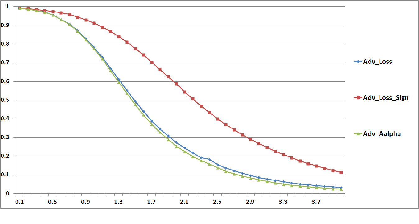
Figure 1: Validation accuracies of different perturbation methods. $x$ axis denotes the $\ell_{2}$ norm of the perturbation.

The networks classification accuracy decreases with increasing magnitude of the perturbation. These results suggest that Adv_Alpha is consistently, but slightly, more effective than Adv_Loss, and these two method are significantly more effective than Adv_Loss_Sign.

Drawback of using $\alpha$ to find perturbations
Note that the difference in perturbation effectiveness between using $\alpha$ and using the loss function is small. On the other hand, to compute the perturbation using $\alpha$, one needs to compute $\frac{\partial\alpha}{\partial x}$, which is $K$ times more expensive than the method using the loss function, which only needs to compute $\frac{\partial\ell}{\partial x}$. (Recall that $K$ is the number of classes.) Due to time limit, during the training procedure we only use the adversarial examples generated from the loss function for our experiments.

4.2 Learning with an adversary

We tested our overall learning approach on both MNIST and CIFAR-10. We measure the robustness of each classifier on various adversarial sets. An adversarial set of the same type for each learned classifier is generated based on the targeted classifier. We generated 3 types of adversarial data sets for the above 5 classifiers corresponding to Adv_Alpha, Adv_Loss, and Adv_Loss_Sign. In addition, we also evaluated the accuracy of these 5 classifiers on a fixed adversarial set, which is generated based on the ‘Normal’ network using Adv_Loss. Finally, we also report the original validation accuracies of the different networks. We use $\ell_{2}$ norm for our method to train the network.

Experiments on MNIST:
We first test different training methods on a 2-hidden-layer neural network model. In particular, we considered: 1. Normal back-forward propagation training, $100\times 100$ (Normal); 2. Normal back-forward propagation training with Dropout, $200\times 200$ (Dropout (Hinton et al., 2012b)); 3. The method in (Goodfellow et al., 2014), $500\times 500$ (Goodfellow’s method); 4. Learning with an adversary on raw data, $500\times 500$ (LWA); 5. Learning with an adversary at the representation layer, $200\times 500$ (LWA_Rep). Here $n\times m$ denote that the network has $n$ nodes for the first hidden layer, and $m$ nodes for the second one. All of the results are tested under perturbations of with the $\ell_{2}$ norm constrained to at most $1.5$.

Table 2: Classification accuracies for 2-hidden-layers neural network on MNIST: the best performance on each adversarial sets are shown in bold. The magnitude of perturbations are $1.5$ in $\ell_{2}$ norm.

METHODS			Validation Sets
	Validation	Fixed	Adv_Loss_Sign	Adv_Loss	Adv_Alpha
Normal	0.977	0.361	0.287	0.201	0.074
Dropout	0.982	0.446	0.440	0.321	0.193
Goodfellow’s Method	0.991	0.972	0.939	0.844	0.836
LWA	0.990	0.974	0.944	0.867	0.862
LWA_Rep	0.986	0.797	0.819	0.673	0.646

We sumarize the results in Table 2. Note that the normal method can not afford any perturbation on the validation set, showing that it is highly non-robust. By training with dropout, both the accuracy and robustness of the neural network are improved, but robustness remains weak; for the adversarial set generated by Adv_Alpha in particular, the resulting classification accuracy is only $19.3\%$. Goodfellow’s method improves the network’s robustness greatly, compared to the previous methods. However, the best accuracy and the most robustness are both achieved by LWA. In particular, on the adversarial sets generated by our methods (Adv_Loss and Adv_Alpha), the performance is improved from $84.4\%$ to $86.7\%$, and from $83.6\%$ to $86.2\%$. The result of LWA_Rep is also reported for comparison. Overall, it achieves worse performance than Goodfellow’s method (Goodfellow et al., 2014) and LWA, but still much more robust than Dropout.

We also evaluated these learning methods on the LeNet model (LeCun et al., 1998a), which is more complex, including convolution layers. We use Dropout for Goodfellow’s method and LWA. The resulting learning curves are reported in Figure 2. It is interesting that we do not observe the trade-off between robustness and accuracy once again; this phenomenon also occurred with the 2-hidden-layers neural network.

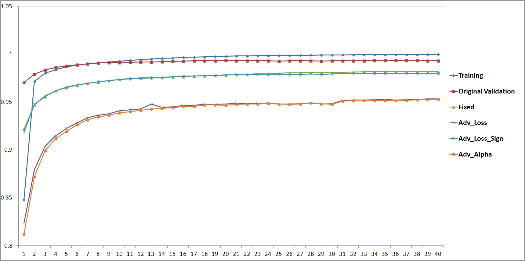
Figure 2: Validation accuracies on MNIST for different perturbation methods. $x$ axis denotes the $\ell_{2}$ norm of the perturbation.

The final result is summarized in Table 3, which shows the great robustness of LWA. We don’t observe the superiority of perturbing the representation layer to perturbing the raw data. In the learned networks, a small perturbation on the raw data incurs a much larger perturbation on the representation layer, which makes LWA_Rep difficult to achieve both high accuracy and robustness. How to avoid such perturbation explosion in the representation network remains open for future investigation.

Table 3: Classification accuracies for LeNet trained using LWA on MNIST. The magnitude of perturbations are $1.5$ in $\ell_{2}$ norm.

METHODS			Validation Sets
	Validation	Fixed	Adv_Loss_Sign	Adv_Loss	Adv_Alpha
Normal	0.9912	0.7456	0.8082	0.5194	0.5014
Dropout	0.9922	0.7217	0.7694	0.5322	0.4893
Goodfellow’s method	0.9937	0.9744	0.9755	0.9066	0.9035
LWA	0.9934	0.9822	0.9859	0.9632	0.9627

Experiments on CIFAR-10:
CIFAR-10 is a more difficult task compared to MNIST. Inspired by VGG-D Network (Simonyan & Zisserman, 2014), we use a network formed by 6 convolution layers with 3 fully connected layers. Same to VGG-Network, we use ReLU as the activation function. For each convolution stage, we use three 3x3 convolution layers followed by a max-pooling layer with stride of 2. We use 128, 256 filters for each convolution stage correspondingly. For three fully connected layer, we use 2048, 2048, 10 hidden units. We also split this network in representation learner and classifier view: the last two fully connected layers with hidden units 2048 and 10 are classifier and other layers below formed a representation learner. We compare the following methods: 1. Normal training (Normal); 2. Normal training with Dropout (Dropout); 3. Goodfellow’s method with Dropout (Goodfellow’s method); 3. Learning with a strong adversary on raw data with Dropout (LWA); 4. Learning with a strong adversary at the representation layer with Dropout (LWA_Rep). We use batch normalization (BN) (Ioffe & Szegedy, 2015) to stabilize the learning of LWA_Rep. We also test the performances of different methods with batch normalization (BN). The results are summarized in Table 4. Learning with a strong adversary again achieves better robustness, but we also observe a small decrease on their classification accuracies.

Table 4: Classification accuracies on CIFAR-10: the best performance on each adversarial sets are shown in bold. The magnitude of perturbations are $0.5$ in $\ell_{2}$ norm.

METHODS			Validation Sets
	Validation	Fixed	Adv_Loss_Sign	Adv_Loss	Adv_Alpha
Normal	0.850	0.769	0.510	0.420	0.410
Dropout	0.881	0.774	0.571	0.480	0.466
Goodfellow’s method	0.856	0.818	0.794	0.745	0.734
LWA	0.864	0.831	0.803	0.760	0.750
Normal + BN	0.887	0.793	0.765	0.747	0.738
Dropout + BN	0.895	0.810	0.729	0.697	0.687
Goodfellow’s method + BN	0.886	0.856	0.821	0.775	0.754
LWA + BN	0.890	0.863	0.823	0.785	0.759
LWA_Rep + BN	0.832	0.746	0.636	0.604	0.574

5 Conclusion

We investigate the curious phenomenon of ’adversarial perturbation’ in a formal min-max problem setting. A generic algorithm is developed based on the proposed min-max formulation, which is more general and allows to replace previous heuristic algorithms with formally derived ones. We also propose a more efficient way in finding adversarial examples for a given network. The experimental results suggests that learning with a strong adversary is promising in the sense that compared to the benchmarks in the literature, it achieves significantly better robustness while maintain high normal accuracy.

Acknowledgments

We thank Ian Goodfellow, Naiyan Wang, Yifan Wu for meaningful discussions. Also we thank Mu Li for granting us access of his GPU machine to run experiments. This work was supported by the Alberta Innovates Technology Futures and NSERC.

Appendix A Analysis of the Regularization Effect of Learning with an Adversary on Logistic Regression

Perhaps the most simple neural network is the binary logistic regression. We investigate the behavior of learning with an adversary on the logistic regression model in this section. Let $\ell(z)=-\log(1+\exp(-z))$. Thus logistic regression is to solve the following problem:

$$\min_{w}\sum_{i}\max_{\|r^{(i)}\|\leq c}\ell(y_{i}w^{\top}(x_{i}+r^{(i)})).$$ (6)

Proposition 4.

The problem 6 is still a convex problem.

Proof.

In fact, there is a closed form solution for the maximization subproblem in (6). Not that $\ell$ is strictly decreasing, thus, Equation (6) is equivalent to

$$\min_{w}\sum_{i}\ell(y_{i}w^{\top}x_{i}-c\|w\|_{*}).$$

Let $h(w)$ denote the concave function of $w$, $y_{i}w^{\top}x_{i}-c\|w\|_{*}$. To prove $\ell(h(w))$ is convex, consider

$$\ell\left(h(w_{1}))+\ell(h(w_{2})\right)\,\geq 2\ell\left(\frac{h(w_{1})+h(w_{2})}{2}\right)\,\geq 2\ell\left(h\left(\frac{w_{1}+w_{2}}{2}\right)\right),$$

where the first inequality is because of the convexity of $\ell$, and the second inequality is because of the monotonicity of $\ell$ and the concavity of $h$. ∎

Let $R_{z}(w)=\max_{\|r^{(i)}\|\leq c}\ell(y_{i}w^{\top}(x_{i}+r^{(i)}))-\ell(y_{i}w^{\top}x_{i})\geq 0$. The behavior of $R_{z}$ is a data-dependent regularization. The next proposition shows that different to common $\ell_{p}$ regularization, it is NOT a convex function.

Proposition 5.

The induced regularization $R_{z}(w)$ is non-convex.

Proof.

An counter example is enough to prove that $R_{z}(w)$ is non-convex. Let $c=0.5$ and $z=(x,y)=(1,1)$, then $R_{z}(w):\real\rightarrow\real$ is

$$R_{z}(w)=\log\left(1+\exp(-0.5w)\right)-\log\left(1+\exp(-w)\right).$$

The figure of this function clearly shows its non-convexity. ∎

One of the common problem about logistic regression without regularization is that there is no valid solution given a linearly separable data set $\underline{Z}$. The following proposition shows that this issue is relieved by learning with an adversary.

Proposition 6.

Assume that the linearly separable data set $\underline{Z}$ has a margin less than $2c$, then logistic regression with adversary is guaranteed to have bounded solutions. Moreover, if $\|\cdot\|_{*}$ is twice differentiable almost everywhere and $\sum_{i}\frac{\partial Q_{i}}{\partial w}\frac{\partial Q_{i}}{\partial w}^{\top}$ is positive definite where $Q_{i}=-y_{i}x_{i}^{\top}w+\|w\|_{*}$, then logistic regression with adversary has unique solution.

Proof.

Since the margin of $\underline{Z}$ is less than $2c$, after the data is perturbed, it is no longer linear separable. Therefore for any $w$, there exists some $i$ such that $-y_{i}w^{\top}x_{i}+c\|w\|_{*}$. Note that $-y_{i}w^{\top}x_{i}+c\|w\|_{*}$ is homogeneous in $w$. Thus, if the optimal solution $w^{*}$ has a infinity norm, then

$$\sum_{i}\log\left(1+\exp(-y_{i}w^{*\top}x_{i}+c\|w^{*}\|_{*})\right)=\infty.$$

However, assigning $w=0$ have finite loss. Therefore, $w^{*}$ is bounded.

Moreover, since $\|\cdot\|_{*}$ is twice differentiable, consider the Hession matrix

$$H=\sum_{i}\frac{e^{Q_{i}}}{(1+e^{Q_{i}})^{2}}\frac{\partial Q_{i}}{\partial w}\frac{\partial Q_{i}}{\partial w}^{\top}+\frac{e^{Q_{i}}}{(1+e^{Q_{i}})^{2}}\frac{\partial^{2}Q_{i}}{\partial^{2}w}.$$

Note that $\|w\|_{*}$ is convex, so is $Q_{i}$. Thus $\frac{\partial^{2}Q_{i}}{\partial^{2}w}$ is positive semi-definite. Since $\sum_{i}\frac{\partial Q_{i}}{\partial w}\frac{\partial Q_{i}}{\partial w}^{\top}$ is positive definite, and $\frac{e^{Q_{i}}}{(1+e^{Q_{i}})^{2}}>0$ for any $i$, $H$ is positive definite. Therefore, the objective function is strictly convex with respect to $w$. Combining the boundedness of $w$ and being strictly convex of $\ell$ leads to the unique of $w^{*}$. ∎

Remark 1.

Unlike adding a regularization term to the objective function, learning with an adversary can only guarantee unique solutions, when the data set is linearly separable with small margin. In such sense, learning with an adversary is a weaker regularization.

References

- Chen et al. (2015) Chen, Tianqi, Li, Mu, Li, Yutian, Lin, Min, Wang, Naiyan, Wang, Minjie, Xiao, Tianjun, Xu, Bing, Zhang, Chiyuan, and Zhang, Zheng. Mxnet: A flexible and efficient machine learning library for heterogeneous distributed systems. arXiv preprint arXiv:1512.01274, 2015.
- Fawzi et al. (2015) Fawzi, Alhussein, Fawzi, Omar, and Frossard, Pascal. Analysis of classifiers’ robustness to adversarial perturbations. arXiv preprint arXiv:1502.02590, 2015.
- Goodfellow et al. (2014) Goodfellow, Ian J, Shlens, Jonathon, and Szegedy, Christian. Explaining and harnessing adversarial examples. arXiv preprint arXiv:1412.6572, 2014.
- Hinton et al. (2012a) Hinton, Geoffrey, Deng, Li, Yu, Dong, Dahl, George E, Mohamed, Abdel-rahman, Jaitly, Navdeep, Senior, Andrew, Vanhoucke, Vincent, Nguyen, Patrick, Sainath, Tara N, et al. Deep neural networks for acoustic modeling in speech recognition: The shared views of four research groups. Signal Processing Magazine, IEEE, 29(6):82–97, 2012a.
- Hinton et al. (2012b) Hinton, Geoffrey E, Srivastava, Nitish, Krizhevsky, Alex, Sutskever, Ilya, and Salakhutdinov, Ruslan R. Improving neural networks by preventing co-adaptation of feature detectors. arXiv preprint arXiv:1207.0580, 2012b.
- Ioffe & Szegedy (2015) Ioffe, Sergey and Szegedy, Christian. Batch normalization: Accelerating deep network training by reducing internal covariate shift. arXiv preprint arXiv:1502.03167, 2015.
- Krizhevsky & Hinton (2009) Krizhevsky, Alex and Hinton, Geoffrey. Learning multiple layers of features from tiny images, 2009.
- Krizhevsky et al. (2012) Krizhevsky, Alex, Sutskever, Ilya, and Hinton, Geoffrey E. Imagenet classification with deep convolutional neural networks. In Advances in neural information processing systems, pp. 1097–1105, 2012.
- LeCun et al. (1998a) LeCun, Yann, Bottou, Léon, Bengio, Yoshua, and Haffner, Patrick. Gradient-based learning applied to document recognition. Proceedings of the IEEE, 86(11):2278–2324, 1998a.
- LeCun et al. (1998b) LeCun, Yann, Cortes, Corinna, and Burges, Christopher JC. The mnist database of handwritten digits, 1998b.
- Miyato et al. (2015) Miyato, Takeru, Maeda, Shin-ichi, Koyama, Masanori, Nakae, Ken, and Ishii, Shin. Distributional smoothing by virtual adversarial examples. arXiv preprint arXiv:1507.00677, 2015.
- Neu & Szepesvári (2012) Neu, Gergely and Szepesvári, Csaba. Apprenticeship learning using inverse reinforcement learning and gradient methods. arXiv preprint arXiv:1206.5264, 2012.
- Nøkland (2015) Nøkland, Arild. Improving back-propagation by adding an adversarial gradient. arXiv preprint arXiv:1510.04189, 2015.
- Simonyan & Zisserman (2014) Simonyan, Karen and Zisserman, Andrew. Very deep convolutional networks for large-scale image recognition. arXiv preprint arXiv:1409.1556, 2014.
- Szegedy et al. (2013) Szegedy, Christian, Zaremba, Wojciech, Sutskever, Ilya, Bruna, Joan, Erhan, Dumitru, Goodfellow, Ian, and Fergus, Rob. Intriguing properties of neural networks. arXiv preprint arXiv:1312.6199, 2013.
- Tabacof & Valle (2015) Tabacof, Pedro and Valle, Eduardo. Exploring the space of adversarial images. arXiv preprint arXiv:1510.05328, 2015.