Alternative search strategies for a BSM resonance fitting ATLAS diboson excess

Abstract

We study an s-channel resonance $R$ as a viable candidate to fit the diboson excess reported by ATLAS. We compute the contribution of the $\sim 2$ TeV resonance $R$ to semileptonic and leptonic final states at 13 TeV LHC. To explain the absence of an excess in semileptonic channel, we explore the possibility where the particle $R$ decays to additional light scalars $X,X$ or $X,Y$. Modified analysis strategy has been proposed to study three particle final state of the resonance decay and to identify decay channels of $X$. Associated production of $R$ with gauge bosons has been studied in detail to identify the production mechanism of $R$. We construct comprehensive categories for vector and scalar BSM particles which may play the role of particles $R$, $X$, $Y$ and find alternate channels to fix the new couplings and search for these particles.

I Introduction

Resonant searches in the s-channel mediated $2\to 2$ process are special as they can provide a smoking gun signal for beyond standard model (BSM) at the LHC. ATLAS collaboration has recently reported a $2.6\sigma-3.4\sigma$ excess in their searches for BSM resonances in diboson channel decaying into two fat jets final states from 20.3 fb^-1 of data at 8 TeV LHCatlasdiboson1 . Any hints in the electro-weak (EW) sector in TeV energy are exciting as almost all the major ultraviolet (UV) completions of Standard Model (SM) predict TeV scale particles. The observed invariant mass distribution of the cross section in diboson channel shows a bump in 1.8-2 TeV region. This gives further support to the weak evidence of an excess of (1$\sigma$-2$\sigma$) which were already seen in the same channels by the CMS experiments in a similar invariant mass regioncmshadronic .

Since the excess arises at  2 TeV scale, the final state gauge bosons($W/Z$) are highly boosted and collimated. In the hadronic decay of a boosted gauge boson, the light quark jets produced are also highly collimated and form one fat jet ($J$). While looking for the two fat jet final states whose jet mass peaks around the $W/Z$ mass, ATLAS found the largest discrepancy near 2 TeV corresponding to 3.4 $\sigma$, 2.6 $\sigma$ and 2.9 $\sigma$ significance in $WZ$, $WW$ and $ZZ$ channels respectively. Considering entire mass range 1.3-3.0 TeV in each of the search channel, the global significance of the discrepancy in the WZ channel is 2.5$\sigma$.

Any BSM particle which decays to two standard model gauge bosons $W/Z$ will also have semileptonic and leptonic final states because of the leptonic decay modes of $W$ and $Z$. Therefore corresponding to the dijet channel, the semileptonic and leptonic channels should also see some excess. However, no such excess has been observed in the searches by CMS or ATLAScmssemileptonic ; cmslllnu ; Aad:2015ufa ; Aad:2014ry ; Aad:2014pl . In the combined analysis of hadronic, semileptonic and leptonic final states, ATLAS finds that the largest deviation from the background expectation is 2.5$\sigma$ and corresponds to a 2 TeV invariant massatlasdiboson2 . This significance is smaller than the 3.4 $\sigma$ significance observed in the JJ channel as the semi-leptonic and leptonic channels are consistent with the background-only hypothesis. We should comment here that the leptonic branching fraction of $W$ and $Z$ are very small, for example in the fully leptonic decay channel, $ZZ$ $\rightarrow$ $4l$, is not very competitive in the diboson resonance search at 8 TeV.

In other related searches, ATLAS and CMS collaborations have presented their results and put upper limits on the $Zh/Wh$ production cross section Khachatryan:2014pqr ; Khachatryan:2015zxd ; Aad:2014lkh . CMS collaboration observes a 2.2 $\sigma$ excess over the standard model at $m_{Wh}$ $\approx$ 1.8 TeV in the $l\nu b\bar{b}$ final stateKhachatryan:2015zxd . Dijet resonance searches also show a (2.1$\sigma$) discrepancy in the invariant mass region of $\approx$2 TeVAad:2014aqa ; Khachatryan:2015sja . Individually these searches have a low statistical significance and may get ruled out with early LHC run IIGoncalves:2015yua . At the same time, the combination of all of these excesses and the appealing signature of TeV scale BSM physics encourage us to look for more ways look for this TeV scale BSM physics in the early LHC run-II.

Naturally, any hint of a discrepancy between SM predictions and observations creates a renewed excitement and a flurry of suggestions for possible explanations and suggestions for further explorations. The possible models which may explain partly or fully, the above experimental results include additional new gauge bosons such as $W^{\prime}$,$Z^{\prime}$WZprime , composite Higgs modelscomposite , heavy Higgs boson(s)Chaostealth ; Chen2tevres ; heavyhiggs , string originated Stringyorigin and $R$-parity violating SUSY modelAllanach:2015blv , walking technicolor Fukano:2015hga and other spin one resonances spin1 . In effective field theory approach for bosonic production is used to study diboson channeldibosoneft .

In this study we explore comprehensively, the production, decay and coupling measurement of a BSM s-channel scalar or vector bosons which can fit the diboson excess. In section II we will review the all experimental results from ATLAS and CMS involving the diboson search. Then, for analysis at 13 TeV LHC, we follow the same strategy as adopted by ATLAS to estimate the number of events in production of $WW,WZ$ and $ZZ$ and their decays to jets, semi-leptonic and leptonic channels. To study BSM models, we start with discussing status of two particle final states coming from the decay of a heavy resonance. Then we check the viability of three particle final state as a possible mimic for the diboson excess. In section III, explore the production mechanism of the heavy resonance to look for probes which distinguish between quark-quark or gluon-gluon initiated processes. We propose alternate channels and cuts to distinguish these two cases in the associated production process. Next we comment on how to independently measure the couplings of the BSM resonance with gauge bosons and quarks. In section IV, we discuss the possibility that, as in the case of 8 TeV, the semi-leptonic and leptonic channels do not show an excess even in the 13 TeV run but in the hadronic decay mode the excess survives. An additional light BSM particle which can mimic the $W/Z$ boson signatures at LHC would be favoured in this scenario. We explore such a model and find general signatures of its decay modes to isolate the BSM physics. In section V, we discuss and categorize simplified models which can accommodate a 2 TeV resonance and additional $W/Z$-like BSM particles with mass $\sim 100$ GeV. In the last section, we discuss some general experimental signatures common to many of the proposed BSM simplified models. In case, this resonance is verified and the LHC run-II confirms its existence with greater statistical significance, following the strategy described in our paper, its couplings and decay modes can be identified in the early LHC run.

II Analysis

In this section we will review ATLAS diboson analysis and CMS results for this diboson excess. ATLAS experiment at LHC has reported diboson excess around 2 TeV in the hadronic decay of gauge bosonsatlasdiboson1 only. They do not see any excess in leptonic channels in their updated analysisatlasdiboson2 . Since gauge bosons coming from the heavy resonance will be very boosted, so their decay products will be highly collimated. Two quarks from hadronic decay of $W/Z$ will form few highly collimated jets which then look like a single jet of bigger radius and these objects are called fat jets. ATLAS has scanned the invariant mass range of $1.3-3$ TeV to look for any BSM resonances decaying to the diboson channel. As the final states are fat jets, in their analysis, jets are constructed using C/A method with radius 1.2. After jet formation, a grooming algorithm, a variant of mass drop technique, is applied to find pair of pair of quarks forming fat jet and to reduce pileup. Mass drop technique is used to examine the sequence of pairwise combinations used to reconstruct the jet to find two subjets corresponding to the $W$ or $Z$ boson decay identified in simulated signal events. Feynman diagram for this process is given in Fig. 1. For semileptonic and leptonic decay channels, in order to maximize the sensitivity to resonances with different masses, three different optimized set of selection criteria are used according to the $p_{T}$ of the leptonically decaying $W(p_{T}^{l\nu})$, $Z(p_{T}^{ll})$ and hadronically decaying $W/Z$ ($p_{T}^{jj}$ or $p_{T}^{J}$ where $p_{T}^{J}$ means the $p_{T}$ of the fat jet). These three regions are low $p_{T}$ resolved, high $p_{T}$ resolved and merged region. As the resonance is 2 TeV, its decay products will be highly boosted and $p_{T}$ of boosted objects will be greater than 400 GeV and high $p_{T}$ merged region is most suitable for this scenario. CMS has not observed any excess and their upper bound on cross-section is given in Table 1. We will discuss ATLAS analysis in detail, results or bounds for each channel one by one.

II.1 Resonance decaying to $WW$, $ZZ$ or $WZ$

Figure 1: Feynman diagram for resonance decaying to two vector bosons.

II.1.1 JJ channel

ATLAS has observed some excess in this channel from 2 TeV resonance decay. This channel is sensitive to $WW$, $ZZ$ and $WZ$ processes. They look for two fat jets with 69.4 $<m_{J}^{W}<$ 95.4 GeV and 79.8 $<m_{J}^{Z}<$ 105.8 GeV, $p_{T}^{J}>$ 540 GeV, $|\eta|<$ 2 and $\frac{p_{T}^{J_{1}}-p_{T}^{J_{2}}}{p_{T}^{J_{1}}+p_{T}^{J_{2}}}$ $<$ 0.15 ($p_{T}^{J_{1}}$ and $p_{T}^{J_{2}}$ denote $p_{T}$ of first and second jet respectively). Only those events are selected when number of charged tracks inside the jets are less than 30 and $\not{E}_{T}$ is less than 350 GeV. Jets having subjets less than 3 are considered. Fat jet pair invariant mass is demanded greater than 1050 GeV. QCD dijet is the largest background for $JJ$ channel and is removed by tagging the vector bosons with

1. $\sqrt{y}>0.5$ for sub-jets (before re-clustering)

2. Number of charged tracks $<30$ for ungroomed jets to remove higher multiplicity gluons

3. $m_{J}\in\left(82.4\pm 13||92.8\pm 13\right)$GeV to tag $W/Z$ bosons

4. $|y_{1}-y_{2}|<1.2$ between 2 leading jets to remove the large t-channel gluon mediated background

In addition to the above cuts, the ATLAS analysis removed events with a prompt electron ($E_{T}>20$ GeV, $|\eta|<1.37$ or $1.52<|\eta|<2.47$) or a muon ($p_{T}>20$ GeV, $|\eta|<2.5$) to avoid overlap with leptonic decay searches in diboson channel and also removed events with $\not{E}_{T}>$ 350 GeV to remove overlap with searches with $Z\to\nu\overline{\nu}$. Limit on diboson cross-section for all the processes corresponding to 2 TeV resonance from ATLAS are given in Table 2.

$$\begin{array}[]{|c|c|c|c|}\hline\cr{\mbox{Upper bound on cross-section}}&{\mbox{WW}}&ZZ&WZ\\ \hline\cr JJ&16&18&16\\ l\nu J&3.5&-&-\\ llJ&-&8.5&-\\ lll\nu&-&-&0.3\\ \hline\cr\end{array}$$

Table 1: CMS 8 TeV diboson bounds on cross-section in fb ($R\rightarrow VV$) for different channels cmslllnu ; cmssemileptonic ; cmshadronic .

$$\begin{array}[]{|c|c|c|c|}\hline\cr{\mbox{Upper bound on cross-section}}&{\mbox{WW}}&ZZ&WZ\\ \hline\cr JJ&30&30&30\\ l\nu J&5&-&9\\ llJ&-&8&20\\ lll\nu&-&-&21\\ \mbox{Combined (hadron + leptonic)}&13&13&15\\ \hline\cr\end{array}$$

Table 2: ATLAS 8 TeV diboson bounds on cross-section ($R\rightarrow VV$) (in fb) for different channels corresponding to $m_{R}$   2 TeV. atlasdiboson1 ; atlasdiboson2 .

II.1.2 l$\nu$J channel

ATLAS has updated analysis of diboson excess also includes leptonic decays of gauge bosons atlasdiboson2 . One can get this final state either from $WZ$ or $WW$ decay. Events which have only one isolated (high $p_{T}$) lepton fall under this category. Following cuts have been used :

1. Jet invariant mass range : $65<m_{W}<105$ GeV and $70<m_{Z}<110$ GeV

2. Lepton $p_{T}$ $>$ 25 GeV

3. Jet $p_{T}^{J}$ $>$ 400 GeV

4. $\not{E}_{T}$ $>$ 30 GeV

5. $p_{T}(l\nu)$ $>$ 400 GeV (vector sum of $p_{T}$ vector of $\not{E}_{T}$ and lepton)

Main backgrounds in this channel are $W$ $+$ jet, top quark pair production and non-resonant diboson production. $\Delta\phi$ cut : $\Delta\phi$ $(\not{E}_{T},J)$ $>$ 1 is applied to reject multi-jet background. Top quark production background is reduced by rejecting the events with b-tagged jet having $\Delta R$ $>$ 0.8 (with fat jet).

II.1.3 llJ channel

This channel is sensitive to $ZZ$ and $WZ$ final state only. All the cuts for this channel are same as previously discussed channels except the condition of same flavour opposite sign dilepton pair. Leptonic pair invariant mass ($m_{ll}$) is required in 65-115 GeV range. Main background processes are $Z$ $+$ jets, top quark pair and non- resonant vector boson pair production.

II.1.4 $lll\nu$ channel

Here three isolated leptons each with $p_{T}$ $>$ 25 GeV and $\not{E}_{T}>$ 25 GeV are demanded. Out of these two leptons should be of same flavour opposite sign. Invariant mass of that pair of leptons should be with in 70-110 GeV ($m_{Z}\pm$ 20 GeV) range since they can be produced only from $Z$ decay. This final state one can get only from $WZ$ decay. Dominant backgrounds for this channel are SM- $WZ$ and $ZZ$ production. Data driven method is used to estimate these background processes.

ATLAS has observed an excess in the $JJ$ channel of gauge boson decay. If the resonance is a true signal, beyond statistical fluctuations, the 13 TeV LHC will be able to see a sharp peak in the $JJ$ channel because the cross-section will increase significantly at 13 TeV. The $JJ$ channel is sensitive to $WW$, $WZ$ and $ZZ$ equally because of same hadronic branching of $W$, $Z$. Therefore from this channel we can’t distinguish whether the resonance is dominantly decaying to $WW$ or $WZ$ or $ZZ$. Hence to comment about its charge we have to be certain about its decay channels. Moreover along with the $JJ$ channel the other decay modes of $W$ and $Z$ i.e. the semileptonic and fully leptonic channels should also observe some clear excess. If the 13 TeV LHC see some excess events in semileptonic or fully leptonic decay channels. We will be able to distinguish which decay mode of the resonance is preferred. For example, the $lll\nu$ channel is only sensitive to $WZ$; $llll$ is sensitive to $ZZ$ only; $l\nu J$, is sensitive to both $WW$ and $WZ$. But significant events in $l\nu J$ channel, and no event in $lll\nu$ will ensure that the final state is $WW$. If they observe no signal in any of the channels, they will be able to rule out the possibility that the resonance decays to diboson final state.

$$\begin{array}[]{|c|c|c|c|c|c|}\hline\cr&\rm{Cuts}&\vrule\lx@intercol\hfil\mbox{No of }\hfil\lx@intercol\vrule\lx@intercol&\mbox{ No. of }\\ &{}\rm\hfil&\vrule\lx@intercol\hfil\mbox{signal}\hfil\lx@intercol\vrule\lx@intercol&\mbox{background}\\ &{}\rm\hfil&\vrule\lx@intercol\hfil\mbox{events}\hfil\lx@intercol\vrule\lx@intercol&\mbox{events}\\ &{}\rm\hfil&\vrule\lx@intercol\hfil\rm{(5fb^{-1})}\hfil\lx@intercol\vrule\lx@intercol&\rm{(5fb^{-1})}\\ \hline\cr{\mbox{Channel}}&&{\mbox{WW}}&ZZ&WZ&\\ \hline\cr l\nu J&p_{T}^{l}>25\,\,\mbox{GeV},\,\,p_{T}^{J}>800\,\,\mbox{GeV},\,\,p_{T}^{l\nu}>800\,\,\mbox{GeV}&65&&30&20\\ \hline\cr llJ&1.8\,\,\mbox{TeV}<m_{llJ}<2.2\,\,\mbox{TeV},\,\,p_{T}^{J}>400\,\,\mbox{GeV},\,\,p^{T}_{ll}>400\,\,\mbox{GeV}&&30&10&2\\ \hline\cr lll\nu&p_{T}^{l_{1}}>100\,\,\mbox{GeV},\,\,p_{T}^{l_{2}}>100\,\,\mbox{GeV},\,\,p_{T}^{l_{3}}>100\,\,\mbox{GeV}&&&4&4\\ \hline\cr llll&p_{T}^{l_{1}}>60\,\,\mbox{GeV},\,\,p_{T}^{l_{2}}>60\,\,\mbox{GeV},\,\,p_{T}^{l_{3}}>60\,\,\mbox{GeV},\,\,p_{T}^{l_{4}}>60\mbox{GeV}&&1&&2\\ \hline\cr\end{array}$$

Table 3: Expected number of events for different leptonic channels at 13 TeV.

To check this, we have done a detailed analysis following the same strategy as ATLAS to calculate the relevant number of events in each channel which will be observed in the 13 TeV LHC. We have also estimated the major backgrounds for all these channels. We used CalcHEPCalcHEP for parton level event generation, Pythia6.4.28pythia for showering and fastjet-3.1.3fastjet for jet formation. Only track isolation is applied to count number of isolated leptons. If the $p_{T}$ sum in cone of radius 0.2 is less than 15 $\%$ of lepton $p_{T}$ then that lepton is declared as an isolated lepton. For $l\nu J$ channel, we have considered $W$ $+$ jets, $Z$ $+$ jets and SM $VV$ production as main background. In case of $llJ$, we have considered $Z$ $+$ $J$ and SM $VV$ production as backgrounds. In case of $llll$, SM $VV$ have been considered as dominant background. The results have been presented in Table 3. We have assumed $R$ $\rightarrow$ $VV$ 100 fb cross-section for $WW$ and also for $ZZ$ and $WZ$ at 13 TeV. In principle these three cross-sections can be different from each other but one can rescale the number of events accordingly. The used optimized cuts to reduce background and to increase signal significance which are also listed in the Table 3.

Expected number of events for this process from $WW,$ $ZZ$ and $WZ$ decay modes are given in Table 3 for 13 TeV LHC. We can see that $WW$ channel can be easily differentiated from the other modes with only 5 fb^-1 of data, because in the $WW$ case, there will be an excess only in the $l\nu J$ channel. To see the events in the fully leptonic channel, we need higher luminosity $\sim$ 100 fb^-1. In case we find some excess in $llJ$ channel but not in $l\nu J$ channel that will definitely correspond to $ZZ$ final state. If one finds excess in both $l\nu J$ and $llJ$ channel then it will be the $WZ$ final state.

Figure 2: Feynman diagram for resonance decaying to two vector bosons and some new particle.

$$\begin{array}[]{|c|c|c|c|c|}\hline\cr M_{Y}&M_{X}&p_{T}^{A}<.15&p_{T}^{A}<.25&p_{T}^{A}<.5\\ {\small{\mbox{(in GeV)}}}&{\small{\mbox{(in GeV)}}}&&&\\ \hline\cr 150.0&10.0&0.28&0.28&0.28\\ 200.0&50.0&0.13&0.13&0.14\\ 300.0&50.0&0.16&0.17&0.17\\ 300.0&100.0&.063&.063&.064\\ 400.0&200.0&.0003&.0003&.0003\\ \hline\cr\end{array}$$

Table 4: Fraction of events passing different $p_{T}^{A}$ asymmetry cuts $\left(\frac{p_{T}^{V_{1}}-p_{T}^{V_{2}}}{p_{T}^{V_{1}}+p_{T}^{V_{2}}}\right)$, 1.8 $<m_{V_{1}V_{2}}<$ 2.2 TeV and $X$ decays invisibly.

$$\begin{array}[]{|c|c|c|}\hline\cr{{M_{Y}}}&{M_{X}}&\mbox{{\small{Fraction of the events}}}\\ {\small{\mbox{(in GeV)}}}&{\small{\mbox{(in GeV)}}}&{\small{\mbox{with}\,\,\Delta R<1.2}}\\ \hline\cr 150.0&10.0&0.97\\ 200.0&50.0&0.97\\ 300.0&50.0&0.86\\ 300.0&100.0&0.92\\ 400.0&200.0&0.87\\ \hline\cr\end{array}$$

Table 5: Fraction of events having $X$ decay products within fat jet radius, for different values of $Y$ and $X$ mass.

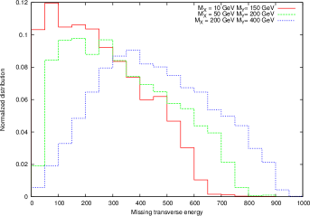
Figure 3: $\not{E}_{T}$ distribution when $X$ decays invisibly for three different sets of $X$ and $Y$ masses as shown in the inset.

So far we have considered 2 $\rightarrow$ 2 topology. Recently it has been argued in saavedra that resonance (which we denote by $R$) can also decay to three particles in the final state as shown in Fig. 2. The schematics of this type of process is $pp$ $\rightarrow$ $V_{1}V_{2}X$. We investigated the viability of this scenario. To this end, we generate parton level events for $R$ decaying to 3 body final state. For this process we have three new particles : $X$, $Y$ and $R$, including the resonance. We want to explore the possibility of this final state mimicking the diboson final state. The particle $X$ can decay into visible or to invisible final states. It can not decay to leptons because that final state is not very difficult to identify. In case $X$ decays invisibly, there will be a $p_{T}$ asymmetry between the visible final states. Hence we calculate the fraction of events respecting different jet $p_{T}$ asymmetry cuts for different combinations of $Y$ and $X$ particle masses. We have taken a few benchmark points for $X$ and $Y$ masses. We have explicitly put the invariant mass cut of 1.8 TeV$<m_{V_{1}V_{2}}<$2.2 TeV on the visible final state particles. We can see from the Table 4 that it is very difficult to satisfy $p_{T}$ asymmetry condition unless $X$ is very light. For $M_{X}$=10 GeV, only 27 $\%$ of the events pass the $p_{T}$ asymmetry cut. But even if this is the case, one can confirm this decay chain by looking at the two fat jets $+$ missing $\not{E_{T}}$ signal (see Fig. 3).

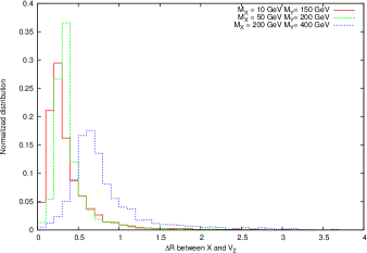
Figure 4: $\Delta R$ distribution between $X$ and $V_{2}$ for three different sets of $X$ and $Y$ masses as shown in the inset.

Second possibility is when $X$ decays to hadrons. Again we look for fraction of events when $X$ lies within ( $\Delta R$ $<$ 1.2 ) fat jet radius (see Fig. 4). We can see from the Table 5 that most of events will pass this condition. Even with high $X$ mass 87 $\%$ of the events will have $X$ and $V_{2}$ ($W$ or $Z$) lying within fat jet radius. In that case, the invariant mass of the two fat jets will also peak around 2 TeV. But still there is a way to rule out this possibility. One of the fat jet invariant mass will peak at $M_{Y}$ instead of gauge boson mass. Low $X$ mass option might pass this criteria. It will be within 1.2 radius and $p_{T}$ asymmetry cut will also not be able to rule out this possibility. But in that case, the jet substructure inside the fat jet will be different. To identify this scenario one has to slightly modify the mass drop technique to look for two parents instead of one and to identify the jet substructure fully when some of the components are not very massive. There can be another possibility that the $X$ lies outside the 1.2 radius and decays into visible particles. But that probability is only about 10$\%$. So we do not consider that possibility here. So if $X$ decays invisibly then low mass $X$ can can pass $p_{T}$ asymmetry cut used by ATLAS and in that case one should look for two fat jets + $\not{E}_{T}$ signal. For visible $X$ decay, ungroomed jet mass $M_{Y}$. One will find more substructure, and more number of tracks inside the fat jet. In that case one should follow different strategy to look for jet substructure.

III Associated Resonance Production

Having discussed the 13 TeV projections of the various leptonic decay modes of the newly observed resonance, we expect that the LHC run II can easily see the resonance through these channels also, and can identify its decay modes precisely. Then one will have clear understanding of decay modes of the 2 TeV resonance. Our next task is to address the issue of production mechanism of this state. Question arises whether the production of the resonance $R$ is a quark initiated or a gluon initiated process. Quarks have tree level gauge couplings with electroweak gauge bosons but these couplings do not exist for gluons. Therefore for quark initiated process we can get gauge bosons $W^{\pm}$, $Z$, $\gamma$ and $g$ (see Fig. 5 for Feynman diagrams) emission from the initial quark legs. Associated production of $R$ with $W,Z,\gamma$ will ensure that the initial state is quark. Gluon has tree level couplings with both quark and gluon. Hence a gluon jet can come from both quark or gluon leg in the initial state initial state (see Fig. 6 (a)), therefore associated gluon production with $R$ can not distinguish the initial states. But if gluon coupling with $R$ exists we will get associated quark jet with $R$ from the process depicted in Fig. 6 (b) also. Using quark/ gluon tagging it may be possible to distinguish these two diagrams. As $W^{\pm}$, $Z$, $\gamma$ can only come from quark initiated process, any signature of the associated production of $R$ with $W^{\pm}$, $Z$ and $\gamma$ will ensure that $R$ is produced through quark coupling. Schematic of associated production is as follows :

$$qq\rightarrow RV\rightarrow WW+W/Z/\gamma\rightarrow JJ+l\nu/ll/\gamma\quad;\quad qq\rightarrow R\rightarrow WW$$ (1)

Typical signals one should look for $RW$ and $RZ$ production at 13 TeV LHC are $JJl\nu$ and $JJl^{+}l^{-}$.

Figure 5: Feynman diagram for quark initiated $RV$ production processes.

Figure 6: Feynman diagrams for associated dijet production.

From this discussion it is evident that associated production of $RV$ is an important channel to explore at the 13 TeV LHC. Hence we will estimate the cross-section for this process. For that one has to specify the model. There have been many analyses based upon spin 0, spin 1 and spin 2 resonance, to explain diboson excess. We consider in our work, a spin 0 resonance, produced through quark initiated process. Having spin information we can find out the viable model parameter space in context of the reported excess. Models with scalar $R$ involve only two couplings i.e. coupling of $R$ with vector bosons ($C_{RVV}$) and R coupling with quarks ($C_{Rqq}$) for $pp\rightarrow R\rightarrow VV$ process. The coupling $C_{Rqq}$ also determines the dijet cross-section. From the dijet resonance searches by ATLAS and CMS at 8 TeV we find that $\sigma(pp\rightarrow R\rightarrow jj)<100$ fb for a 2 TeV resonance Aad:2014aqa ; Khachatryan:2015sja . Our aim is to look for parameter space consistent with both diboson and dijet constraints. We find that to satisfy dijet cross-section limit $C_{Rqq}<0.33$. As mentioned the process $pp\rightarrow R\rightarrow VV$ involves both $C_{Rqq}$ and $C_{RVV}$ coupling and its cross-section is proportional to product of these two couplings. The ATLAS upper limit on the diboson cross section is $\approx 10$ fb atlasdiboson1 at 8 TeV (We use average of cross-section limits from CMS and ATLAS). In Fig. 7 we show contours of constant $\sigma(pp\rightarrow R\rightarrow VV)$ in the $C_{Rqq}$ and $C_{RVV}$ plane. The whole parameter space shown in Fig. 7 is compatible with the 8 TeV dijet constraintsAad:2014aqa ; Khachatryan:2015sja . The red dotted line denotes the contour which gives the diboson $\sigma(pp\rightarrow R\rightarrow VV)$ $\approx$ 10 fb which is the upper limit on the diboson cross section from ATLAS. So parameter space below this curve is allowed by diboson search. We have plotted the projected limit for 14 TeV LHC for the dijet cross section Yu:2013wta . The red solid line in the Fig. 7 is the projected dijet limit for 14 TeV. Only the region to the left of this line will be allowed by the dijet search at 14 TeV. Assuming $Z^{\prime}_{B}$ model, 14 TeV limits on $Z^{\prime}$-quark coupling has been calculated in Yu:2013wta . Using this limit, we have calculated 14 TeV projected limit on dijet cross-section which we used to extract the 14 TeV limit on the $C_{Rqq}$ coupling in our model, corresponding to 300 fb^-1 luminosity. We can see from the figure that 14 TeV LHC can rule out most of the currently allowed parameter space.

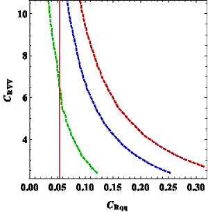
Figure 7: Contours of constant $\sigma(pp\rightarrow R\rightarrow WW)$(fb) in $C_{Rqq}$ $C_{RVV}$ plane. The maroon, blue and green dotted curves denote 10 fb, 5 fb and 1 fb cross-section contours respectively. The red solid line is the projected dijet bound at 14 TeV.

We have chosen few benchmark points $(C_{Rqq},C_{RVV})$ from the allowed parameter space. In Table 6 we quote the 13 TeV associated $RV$, dijet and associated dijet cross-section for the benchmark points.

Now our objective is to present a projection of the associated production of $R$ with gauge bosons for 13 TeV LHC. Using first benchmark($C_{Rqq}=0.3$, $C_{RVV}=2.67$) point we have generated 20,000 parton level events for $pp\rightarrow RW$ and $RZ$ processes, using CalcHEP. We pass these events to Pythia 6.4.28 for hadronization and used fastjet for jet formation. Main backgrounds for these processes are $W/Z$ $+$ jets. To ensure that the lepton(s) coming from $W$/$Z$ are isolated and well separated from the decay products of the high $p_{T}$ gauge bosons, we plot $\Delta R$ distribution between $W$ and $R$ in Fig. 8 (a). $W$ boson $p_{T}$ distribution for associated $RW$ is given in Fig. 8 (b). One can see from these two figures that the lepton will be indeed isolated and it will carry enough $p_{T}$ such that this can be a clear signal to identify at LHC. We estimate the number of events for $JJl\nu$ and $JJll$ processes for 13 TeV LHC run. All our cuts are same as $JJ$ channel of ATLAS diboson analysis except for the $JJ$ invariant mass cut which we consider in the range 1800-2200 GeV in this case. Diboson signal strength will be maximum in the narrow region around 2 TeV. For associated $RW$ production in the $JJl\nu$ final state we have used the following cuts :

$$\begin{array}[]{|c|c|c|c|}\hline\cr{{C_{Rqq},C_{RVV}}}&(0.3,2.67)&(0.09,10.13)&(0.11,7.99)\\ \hline\cr\sigma(RW)&75.6\,\,\mbox{fb}&6.8\,\,\mbox{fb}&10.26\,\,\mbox{fb}\\ \sigma(RZ)&32.4\,\,\mbox{fb}&3.02\,\,\mbox{fb}&4.42\,\,\mbox{fb}\\ \sigma(R\gamma)&4.24\,\,\mbox{fb}\,\,(p_{T}>20\,\,\mbox{GeV})&0.72\,\,\mbox{fb}\,\,(p_{T}>20\,\,\mbox{GeV})&1.14\,\,\mbox{fb}\,\,(p_{T}>20\,\,\mbox{GeV})\\ \sigma\mbox{(dijet )}&470.0\,\,\mbox{fb}&1.44\,\,\mbox{fb}&4.8\,\,\mbox{fb}\\ \sigma\mbox{(associated dijet)}&57.6\,\,\mbox{fb}&0.16\,\,\mbox{fb}&0.6\,\,\mbox{fb}\\ \hline\cr\end{array}$$

Table 6: 13 TeV cross-section estimate for different processes for three benchmark points.

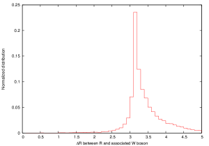
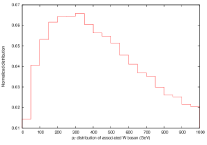
Figure 8: (a) $\Delta R$ distribution between $R$ and $W$, (b) $p_{T}$ distribution of $W$ produced in association with $R$.

1. $30<p_{T}^{l}<350$ GeV

2. $30<\not{E_{T}}<350$ GeV

For associated $RZ$ decaying to $JJll$ final state only the lepton $p_{T}$ cut is used. Expected number of events for $JJl\nu$ and $JJll$ are given in Table 7 and 8 respectively.

$$\begin{array}[]{|c|c|c|}\hline\cr{{\sqrt{s}}}&{\rm{8TeV}}&{\rm 13TeV}\\ \hline\cr{\rm{Total\,\,No.\,\,of\,\,Generated\,\,Events}}&20000&20000\\ \hline\cr\sigma(pp\rightarrow RW)&5\,\,\mbox{fb}&75.6\,\,\mbox{fb}\\ \hline\cr JJl\nu&277&161\\ \hline\cr\end{array}$$

Table 7: Expected number of events for $JJl\nu$ from $RW$ associated production using the first benchmark points for couplings $C_{Rqq}$=0.3 and $C_{RVV}$=2.67.

$$\begin{array}[]{|c|c|c|}\hline\cr{{\sqrt{s}}}&{\rm{8TeV}}&{\rm 13TeV}\\ \hline\cr{\rm{Total\,\,No.\,\,of\,\,Generated\,\,Events}}&20000&20000\\ \hline\cr\sigma(pp\rightarrow RZ)&2.2\,\,\mbox{fb}&32.0\,\,\mbox{fb}\\ \hline\cr JJll&101&69\\ \hline\cr\end{array}$$

Table 8: Expected number of events for $JJll$ from $RZ$ associated production using using the first benchmark points for couplings $C_{Rqq}$=0.3 and $C_{RVV}$=2.67.

If the resonance is produced through quark initiated process then 13 TeV LHC will be able to confirm that looking at associated production of $R$ with gauge bosons in the 2 fat jets $+$1 lepton $+\not{E_{T}}$ in case of associated $RW$ and a pair of leptons with 2 fat jets in case of associated $Z$ production. $RW$ is the best channel to look for, since $W$ branching to lepton is much higher than $Z$ branching ratio to the leptons which is clear from the Table 7 and 8. The backgrounds for these processes are found to be negligible.

Figure 9: Feynman diagram for resonance decaying to three vector bosons.

Although we have argued that looking at associated production of $R$ with gauge bosons is is the best strategy to identify the production mechanism of $R$, we should also mention that a 2 $\rightarrow$ 3 process where R decays to $WWZ$ (s-channel diagram - see Fig. 9) will give us the same signature as the associated production $RZ$ (where $R(\rightarrow WW)Z$) or $RW$ ($(R\rightarrow WZ)W$). This process can come from quark quark as well as gluon gluon final states. Hence looking at only associated production of $R$ with gauge bosons is not enough to comment about the production mechanism of $R$. The typical cross section for this type of processes is 0.5 fb and 4 fb approximately at 8 TeV and 13 TeV respectively for the first benchmark point($C_{qqR}$=0.3 and $C_{RVV}$=2.67. We can see from Table 6 we can see that the cross section of this process is much smaller than the typical $RW$ or $RZ$ associated production cross section. There are one more efficient way to distinguish between these two cases. In addition to looking for leptonic signals with two fat jets, one should also count the number of positive and negative charged leptons in this process. We will always find some asymmetry in the lepton number count if it is a quark initiated process. The reason behind this is that the cross-section of $u\bar{d}\rightarrow RW^{+}$ and $d\bar{u}\rightarrow RW^{-}$ is different in proton-proton collider. Absence of total lepton charge asymmetry will reflect the possibility that we are looking at three gauge boson final state, produced through $R$ decay, through s-channel production of $R$ ( see Fig. 9). Hence looking at the associated production of $R$ with $W$ as well as counting the number of positive and negatively charged leptons one can be definite about the production process of $R$.

The s-channel production of $RW$ or $RZ$ which also has the same final state as the associated production is not important, because its cross section is of $10^{-5}$ fb.

As one of our objective to extract the couplings $C_{qqR}$ and $C_{RVV}$, we have looked at two other processes which involve such couplings. Diboson production gives an upper bound on the product of $C_{qqR}$ and $C_{RVV}$ as discussed earlier. We have given dijet and associated dijet production cross section for a few benchmark points. These two processes depend only on the $C_{qqR}$ coupling and if we can extract this coupling from their cross section we will be able to comment on $C_{RVV}$ coupling. Feynman diagrams for associated dijet production are given in Fig. 6. We should comment here that the dijet production process has large QCD background. Hence coupling measurement from this channel has a lot of uncertainty. Associated dijet production is contaminated with less background. Hence this channel is better to extract couplings.

IV Resonance decaying to two BSM particles

In section III, we have analyzed the number of events in all the leptonic final states coming from the decay of $WZ$, $WW$ and $ZZ$. The semi-leptonic and fully leptonic final states being extremely clean we show the expected signal in these channels at the 13 TeV LHC in Table  3. Observation of these events will confirm that a resonance actually decays into a pair of gauge bosons. If we do not see any excess in the semi-leptonic and leptonic decay channels of gauge boson at 13 TeV and the hadronic signature of BSM appears again, it would rule out a model which decays to $W/Z$ bosons alone. In such a case, an additional particle $X$ (see Fig. 11) with a mass in the 70-100 GeV range which decays to light quarks/gluons will be required to explain this excess. The possible decays of particle $X$ are discussed below,

1. It can decay to light quarks or gluons.

2. $b\bar{b}$ final state. In which case, with b-tagging of the fat jets one will be able to identify this final state. We should comment here that the b-tagging efficiency will be less for high $p_{T}$ jets ($<50\%$)btagging . Still, it is possible to count number of b-subjets inside fat jets.

3. $X$ can also decay into pair of $\tau$ leptons. This decay mode can not be dominant decay channel of $X$ otherwise we will see some excess in the leptonic channels of diboson searches through tau decay. We can observe ditau tagged (boosted) fat jets and identify this final state also.

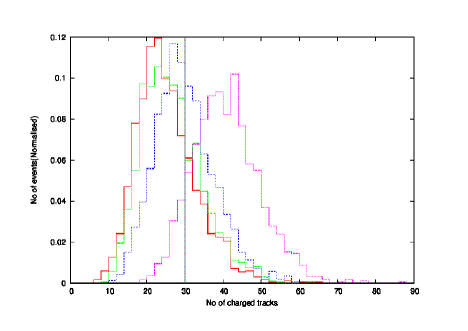
Figure 10: Normalized charge multiplicity distribution for highest $p_{T}$ jet formed by different ($u\bar{u}$- red, $c\bar{c}$- green, $b\bar{b}$- blue and $gg$- violet) decay modes of particle $X$.

We have studied in detail different scenarios, where $X$ can decay into gluons or quarks. Using Pythia6.4.28, tune (AUET-2B) and pdf-CTEQ6L1, we have simulated the listed decay channels of the particle $X$. In Fig. 10, we show number of charge tracks in the fatjet with $p_{T}$ $>$ 540 GeV coming from $u\bar{u}$, $c\bar{c}$, $b\bar{b}$ and gluon -gluon final states for comparison. If it decays to gluons then one finds more number of charge tracks in a fat jet as compared to quark jetsquarkgluon . As the ATLAS experiment puts a cut that number of charge tracks $<30$ inside a fat jet, the gluon final state as should not be the dominant decay mode of $X$ to avoid reduction in the cross section via the branching fraction. Additionally, with the experimental cuts, signal selection efficiency in case of gluon jets is very small (20 $\%$) and we need high cross-section to observe this final state. It is very difficult to distinguish $u\bar{u}$, $c\bar{c}$ and $b\bar{b}$ final states from charge track distribution, unless the b-jets are tagged. As mentioned earlier, in the high $p_{T}$ regions, b-tagging efficiency is lower. Once we have enough data, we can see b-jet sub-jets in the fat jets. When one $X$ decays to quarks and the other to gluons, this scenario can be identified within low luminosity because quark-quark final state has more signal selection efficiency, as shown in the Fig. 10.

The particle $X$ can be tracked via its decay modes discussed above at early LHC run-II. The gluon fraction in the final state can be checked by changing (increasing) the number of charge track cut on the fat jet. For dijet final state the QCD background also becomes large when this cut is relaxed but associated production scenario, discussed in the previous section because of less background it may form a viable channel for the final state analysis.

Figure 11: Feynman diagram for resonance decaying to pair of particle $X$.

V Anatomy of models explaining diboson excess

In order to fit to the bump observed in the data, s-channel models are favored. In the following section, we will explore a number of viable s-channel BSM models and discuss them in the context of diboson excess and associated processes at LHC.

While building s-channel models, we limit to a 2 body or 3 body final states. This is because, a larger number of particles in the final state would suppress the cross section due to phase space factors and also due to the kinematic cuts, for example, the requirement of jet $p_{T}$ asymmetry within $15\%$atlasdiboson1 . Hence, three topologies exist which can mimic the excess in the diboson data as shown in Fig. 12.

Figure 12: Topologies of s-channel BSM resonance.

In all of the considered models, a 2 TeV particle ($R$) is produced in either a quark initiated or a gluon initiated process. The mediating particle $R$ can be a scalar, vector or a spin 2 boson. Next, we discuss the production of the particle $R$ with a gluon or quark initial state.

V.1 Production

$R$ can interact with quarks via tree level couplings whereas gluons may interact with $R$ via a 5 or 6 dimensional effective operator. Below, we discuss both of these possibilities in detail.

Gluon initiated process: Here the particle $R$ is produced from gluon fusion initial state. The Kronecker product $8\times 8$ of the color representations of gluon initial state dictates that the particle $R$ can belong to a 1, $8$, $10$, $\overline{10}$ or $27$ dimensional representation of $SU(3)$ Slansky:1981yr . Firstly, we consider the possibility that $R$ is a vector boson. The SM gluon clearly will not satisfy the role of $R$ since it is massless. The case where the BSM gauge boson is singlet under $SU(3)_{C}$, the lowest dimensional operator for its interaction with the gluon is, $G_{\mu\nu}G^{\mu\nu}F^{\prime}_{\alpha\beta}F^{\prime\alpha\beta}$, where $F^{\prime}_{\alpha\beta}$ is the field strength of R. Such a particle cannot be produced singly from gluon initial state and hence cannot belong to any of the topologies considered.

Next, we consider the case where $R$ is a scalar field. From the point of view of production of a scalar $R$, any of the above color representations are allowed. As we will note later, the required final state will rule out all the colored representations of a scalar particle $R$. This leaves, for a color-singlet scalar, two choices of effective interactions with the gluon,

1. $G_{\mu\nu}G^{\mu\nu}R,$

2. $G_{\mu\nu}G^{\mu\nu}R^{\dagger}R$.

In the first case, $R$ is a singlet under SM gauge group. In the second case $R$ may have non-trivial representations under $SU(2)\times U(1)$. However, in this case, $R$ has to get a non zero vacuum expectation value (VEV) to obtain a $ggR$ vertex. In addition, tree-level corrections to the $\rho$-parameter constraint $R$ to belong to one of the 1, 2 or 7 dimensional representation of $SU(2)\times U(1)$Bhattacharyya:2009gw .

Quark initiated: The case where $R$ is a vector gauge boson, the SM gauge group is extended with additional symmetries. In principle, a UV completion of SM can be complicated, though, at the TeV scale, BSM gauge particles interacting with quarks have similar signatures as $W^{\prime}$ or $Z^{\prime}$ models. These possibilities have been amply explored in the literature and we limit to the alternative where $R$ is a scalar. For a scalar $R$, possibilities for its couplings with the quarks are listed in Tab. 9. Here, we list up to dimension six operators along with the corresponding SM gauge representation of R denoted as (SU(3),SU(2),U(1)). The hypercharge listed in the Table 9 is defined in a convention where Higgs boson has hypercharge $\frac{1}{2}$.

Operator	Representation of $R$
Renormalizable interactions
$Q_{L}^{T}CQ_{L}R$	$\left(\bar{6},3,\frac{1}{3}\right),\left(\bar{6},1,\frac{1}{3}\right),\left(3,3,\frac{1}{3}\right),\left(3,1,\frac{1}{3}\right)$
$u_{R}^{T}Cu_{R}R$	$\left(6,\bar{3},-\frac{4}{3}\right),\left(6,1,-\frac{4}{3}\right),\left(\bar{3},3,-\frac{4}{3}\right),\left(\bar{3},1,-\frac{4}{3}\right)$
$d_{R}^{T}Cd_{R}R$	$\left(6,\bar{3},\frac{2}{3}\right),\left(6,1,\frac{2}{3}\right),\left(\bar{3},3,\frac{2}{3}\right),\left(\bar{3},1,\frac{2}{3}\right)$
$\bar{Q}_{L}u_{R}R$	$\left(8,2,-\frac{1}{2}\right),\left(1,2,-\frac{1}{2}\right)$
$\bar{Q}_{L}d_{R}R$	$\left(8,2,\frac{1}{2}\right),\left(1,2,\frac{1}{2}\right)$
Higher dimensional
$\left(\bar{Q}u_{R}\tilde{H}\right)R,\,\left(\bar{Q}d_{R}H\right)R$	$\left(8,1,0\right),\,\left(1,1,0\right)$
$\left(\bar{Q}u_{R}\tilde{H}\right)R^{\dagger}R,\,\left(\bar{Q}d_{R}H\right)R^{\dagger}R$	$\left(1,1,0\right),\left(1,7,\pm 2\right)$
$\left(\bar{Q}u_{R}H\right)R$	$\left(8,3,-1\right),\left(8,1,-1\right),\left(1,3,-1\right)\left(1,1,-1\right)$
$\left(\bar{Q}d_{R}\tilde{H}\right)R$	$\left(8,3,1\right),\left(8,1,1\right),\left(1,3,1\right)\left(1,1,1\right)$
$\left(\bar{Q}u_{R}\tilde{H}\right)R^{\dagger}R,\,\left(\bar{Q}d_{R}H\right)R^{\dagger}R$	$\left(1,1,0\right),\left(1,7,\pm 2\right)$
$\bar{q}\cancel{D}qR$	$\left(1,1,0\right)$
$\bar{q}\cancel{D}qR^{\dagger}R$	$\left(1,1,0\right),\left(1,7,\pm 2\right)$

Table 9: Quark couplings with a scalar particle $R$

This completes our discussion of the production of the particle $R$.

V.2 Explicit models for $2\to 2$ topology

The final state particles that $R$ decays into may be SM ($W,Z$) or BSM particles of similar mass as $W/Z$ bosons. We call the class of models where the final state particles are SM EW gauge bosons $W/Z$ as $RVV$ models. $R$ may decay into $WW$, $ZZ$ and $ZW$ final states. This class contains some of the minimal extensions of the SM. We arrive at another possibility when one of the out going particles is $Z$ or $W$ and other particle is a BSM particle denoted as $RVX$ models. Remaining two possibilities arise when all the outgoing particles are BSM particles, denoted $RXX$ and $RXY$ models, where, in the later case the two final state particles are different.

V.2.1 RVV models

The resonant particle $R$ must be a colorless particle as the $W$ and $Z$ bosons do not carry any color. There are only three such possibilities for scalar $R$: singlet, Higgs-like $SU(2)$ doublet and a seven dimensional representation $(1,7,\pm 2)$. The collider signature of a vector boson $R$ is similar to either $W^{\prime}$ or $Z^{\prime}$ type models.

A weak and color singlet scalar $R$ heavyhiggs can be produced through both quark and gluon initiated processes. For a gluon initiated process $R$ must be electrically neutral. An electrically neutral scalar singlet $R$ can decay to $WW$ and/or $ZZ$ through mixing of $R$ with CP even Higgs ($h$) or through the following higher dimensional operators,

$$W_{\mu\nu}^{a}W^{\mu\nu}_{a}R,B_{\mu\nu}B^{\mu\nu}R,$$ (2)

where $a=1,2,3$.

For the case where $R$ is a Higgs like doublet, both the quark and gluon initiated production of $R$ are possible Chen2tevres ; heavyhiggs ; WZprime . In addition, the 2HDM also fits, via the charged heavy Higgs, an excess in the search for resonances in $W^{+}h$ channelChaostealth .

The third possibility where $R$ is an SU(2) seven dimensional scalar is very distinct as it contains exotic charged fields with charges $\pm 5,\pm 4,\pm 3,\pm 2,\pm 1$ along with the neutral $R$.

V.2.2 RVX, RXX and RXY models:

The advantage of introducing non-minimal extensions of SM to explain the observed diboson excess is that the constraints that apply from leptonic and semi-leptonic channels can be partially or fully evaded with non-universal couplings with the BSM. In order to pass the experimental cuts for diboson channel, the masses of the additional final state particles $X$ and $Y$ range from $69.4{\,\rm to\,}104.8$ GeV. This also implies that they cannot be colored particles due to dijet constraints. As $W,Z,X$ and $Y$ are all non-colored, R must also be colorless. $RXX$ models, even though exotic, allow an explanation for why the experiments see an excess in the fully hadronic final state of the diboson channel and not in the semi-leptonic and leptonic final states.

Next, considering the case where $R$ is a scalar particle which interacts with the quarks, there are 4 possibilities for it’s EW properties,

1. singlet: $\left(1,1,0\right),\left(1,1,\pm 1\right)$ ,

2. $SU(2)$ doublet like Higgs,

3. $SU(2)$ triplets $\left(1,3,\pm 1\right)$, and

4. the seven dimensional field with representation. $(1,7,\pm 2)$.

The final state particles $X$ and $Y$ in a subset of the models below decay into quark jets and mimic the massive vector boson decay-jets. $X,Y$ may also decay to gluons via effective couplings and may be searched for in this channel. These events are excluded in the diboson analyses due to cuts on number of charged tracks in a jet. The above list of representations, therefore applies to both of these particles as well. In the case where any of the $R,X,Y$ scalars is an SU(2) triplet, in order to avoid tree level corrections to the $\rho$ parameter, this scalar has a 0 VEV.

Singlet scalar $R$: Consider the possibility that $R$ is a singlet scalar. In a model of type $RVX$, $X$ can be a singlet, doublet or 7 dimensional representation of SU(2). Upon symmetry breaking, mixing between neutral scalar bosons allows the $R\to VX$ final state. Similarly, through trilinear couplings arising from the scalar potential after electroweak symmetry breaking, $RXX$ and $RXY$ type models can also be formulated.

SU(2) doublet $R$: When $R$ belongs to an EW doublet, $RVX$ type models can be formulated, where the final state particle $X$ may be any particle from the list above. Since X has a mass similar to the $W/Z$ boson it’s multiplet contains a light charged scalar which is constrained from the process $b\to s\gamma$Gambino:2001ew . These constraints can be evaded with large quartic couplings and mass splittings within the $X$ multiplet after symmetry breaking. When $X$ is a singlet, a small mixing with Higgs implies that the coupling of $RWX$ is small and R needs a larger coupling with quarks/gluon to match the required production cross section. $RXX$ and $RXY$ type models can also be constructed with trilinear couplings arising from the scalar potential. When $X/Y$ has a non zero VEV, the mass matrix of neutral scalars has to be diagonalized with two eigenvalues with a large separation. This complication can be avoided with a zero VEV for $X$ and $Y$. In models with multiple Higgs like doublets, the constraints due to mass splittings become weaker. As an example, in MSSM there are five scalar doublets, two from the Higgs superfields and three from lepton superfields which can have the required low mass scalar as well as a 2 TeV resonant scalarAllanach:2015blv .

SU(2) triplet $R$: Similar to the case where $R$ is a singlet, $RVX,RXX$ and $RXY$ type models can be defined where the triplet particles do not get a VEV. In this case, masses of the zero VEV scalars are obtained as bare masses.

Seven dimensional $R$: This is an exotic case where a number of multi-charged particles of TeV scale mass arise along with the particle $R$. In the case of $RVX,RXX$ and $RXY$, the particle X may be a singlet, doublet or 7 dimensional representation of EW symmetry. Additionally, $RXX$ and $RXY$ models can also be constructed with a triplet $X,Y$. The special case of 7 dimensional $X,Y$ is possible from the perspective of constraints from the $\rho$ parameter, however, a number of light, multi-charged scalars are present in the BSM spectrum which are constrained.

Gauge boson $R$: When $R$ is a gauge boson, consider the $RXX$ coupling, if X is a gauge field, then we obtain a non minimal extension of SM with two new symmetry groups. This possibility is disfavored as, if $X$ belongs to a U(1) group, $RXX$ coupling does not exist, on the other hand, if $X$ belongs to a non abelian group, anomaly cancellation requires addition of multiple generations of new fermions. $RVX,RXX$ and $RXY$ type models can be constructed when $X,Y$ belong to any of the scalar representations listed above.

V.2.3 Some aspects of $2\to 3$ topology

In this topology, the final state is such that two of the particles mimic the signal obtained from $W/Z$ bosons and the third particle is not detected with the CMS/ATLAS diboson analyses cuts. This requires the mass of the third hidden particle to be $\lesssim 100$ GeV otherwise large loss in invariant mass or $p_{T}$ asymmetry would not pass the experimental cuts. In the case where, $R,X$ and $Y$ are either singlets or doublets, in addition to the $2\to 2$ process, the $2\to 3$ process can also, in certain kinematic regimes, provide a signal to the diboson channel. Here we point out that all the models which attempt to explain the diboson excess with a 3 body final state suffer from a set of common constraints. With more number of massive particles in the final state, the phase space suppresses the cross section. The kinematic cuts which ensure that the two fat jets in the final state have a small relative $p_{T}$ and large separation also add further suppression in this topology. The couplings need to be very large to get a large enough total cross section that after the cuts, the required diboson excess is satisfied.

V.3 Experimental signatures

Dijet channel at LHC provides a lower bound on the coupling and masses of any BSM particle that couples to quarks or gluons. This constraint would apply to all the proposed $R$ particles and, via the effective couplings with the quarks, to the final state particle $X$ as well. Another interesting channel which has been discussed in detail in a previous section is that of associated production of $R$ with gauge boson. This channel also provides crucial information about the production mechanism of $R$. In the case where $R$ is produced via a quark initiated process, the total charge of the final state leptons integrated over all the events is positive. However, in the case of gluon initiated process, this number would be 0. This channel provides an independent probe into the $RVV$ type BSM models which can constrain them even with low luminosity ($\sim 5\,fb^{-1}$), early results from LHC-13. In particular, models where the particle $X$ decays to $b\bar{b}$ or $\tau^{+}\tau^{-}$, the branching fraction (BF) to bottom quark should be large and accessible to b-tagged searches at the LHC. Also, the spin of the particle $X$ in the $RXX$ model can be observed through energy fractions of the sub-jets in reconstruction of the $W/Z$-like particles in the diboson search. Angular correlations of $X$ reconstructed jets can in-turn be used to determine the spin of $R$ once larger data points are available in the high invariant mass region. The BF to tau cannot be large to avoid a significant contribution to the semi-leptonic channel in the diboson searches where no BSM has been observed. In the models where the BSM scalar transforms under a 7 dimensional representation of SU(2), searches for doubly charged Higgs with $T_{3}=0$ limit the mass of such a particle to $m_{H}^{++}\geq 322$ GeV at 95% C.L. ATLAS:2012hi . Due to this limit, a light neutral scalar $X$ cannot belong to a higher dimensional representation of SU(2) group since the mass splitting among the neutral and charged Higgs requires one neutral scalar to be heavier.

VI Summary

With the recently observed excess in the resonance searches in diboson channel at the LHC 8 TeV run, we have analyzed the phenomenological signatures of the BSM physics to isolate it in the observed events and provide complimentary signatures for LHC-13 searches. Analysis of the decay channels of diboson process reveals that in the early LHC 13 TeV run, within $\sim 5fb^{-1}$ of data, it would be possible to confirm the existence of a BSM particle which fits the observed excess. In addition, we show that, based on the relative measurements in semi-leptonic and leptonic channels, as shown in Table 3, it will be possible to distinguish between BSM physics contributions to $WW$, $WZ$ and $ZZ$ channels.

The resonance $R$ proposed to fit the diboson excess may be generated via a quark initiated or a gluon initiated process. The process of associated production of EW gauge bosons with $R$ can identify the initial state and provide an independent probe into the nature of couplings of $R$. The particle $R$ will also contribute to the dijet process ($pp\to R\to jj$) and the associated dijet process ($pp\to RV\to jjV$) . When $R$ couples with gluons, the final state $R+j\to jjj/VVj$ is also possible. Combining these processes provides a way to constrain all the couplings of $R$ with SM particles.

Since no excess has been observed in the semi-leptonic channel, we also explore a non-minimal model compatible with this observation. We add an additional particle denoted as $X$ with a mass $\sim 100$ GeV which primarily decay mode into hadronic final states. This particle can mimic the $W/Z$ signature searched by the experiments and satisfy the observed excess. We discuss the decay modes of $X$ into $\bar{q}q$, $g$g, $\bar{b}b$ and $\tau^{+}\tau^{-}$. A cut on the number of charged tracks ($<30$) implies that $X\to gg$ cannot be the primary decay mode. An analyses of the diboson search with a relaxed cut on number of charged tracks may add the gluon channel increasing the statistical-significance of the excess. A boosted b-tagging or ditau tag would also allow isolation of these decay channels of $X$.

In addition, we consider a different topology of models with 3 particles in the final state, denoted as $RXY$ models with the decay chain, $pp\to R\to VY\to VVX$ where V is the $W/Z$ boson. The final state particle, $X$ can be invisible or can decay hadronically. The former case successfully fits the diboson excess only for small masses $m_{X}\approx 10$ GeV. For larger values of mass of $X$, the $p_{T}$ asymmetry of the two final state gauge bosons becomes too large to pass the experimental cuts. This type of invisible particle can be identified in the boosted diboson fat jets + MET process. If $X$ dominantly decays hadronically, it is a part of the boosted fat jet in the final state. Here, we expect to get more sub-jets in one of the fat jets, and may be identifiable by the two mass drops within the reconstructed jet.

In case that LHC-13 indeed finds evidence to support the presence of BSM physics in the EW sector, the possible models can be divided into categories based on their couplings with the qq/gg initial state and EW gauge bosons. We discuss the anatomy of the BSM physics which can explain the diboson excess and categorize the possible s-channel resonances into simplified models and list the couplings. The coupling of $R$ with the EW gauge bosons fixes it’s SM gauge symmetries to a colorless, SU(2) singlet, doublet, or a 7 dimensional representation.

Finally, our results are applicable to general models which attempt to explain the diboson excess and will enable early detection of the BSM physics at LHC run-II. If the resonance studied here is indeed found at LHC-13, analyses of multiple channels which receive contributions from it will be essential tools to fix the spin, charge and couplings of the BSM particle(s).

VII acknowledgements

Work of B. Bhattacherjee is supported by Department of Science and Technology, Government of INDIA under the Grant Agreement numbers IFA13-PH-75 (INSPIRE Faculty Award).

References

- (1) G. Aad et al. [ATLAS Collaboration], arXiv:1506.00962 [hep-ex].
- (2) V. Khachatryan et al. [CMS Collaboration], JHEP 1408, 173 (2014) [arXiv:1405.1994 [hep-ex]].
- (3) V. Khachatryan et al. [CMS Collaboration], Phys. Lett. B 740, 83 (2015) [arXiv:1407.3476 [hep-ex]].
- (4) V. Khachatryan et al. [CMS Collaboration], JHEP 1408, 174 (2014) [arXiv:1405.3447 [hep-ex]].
- (5) G. Aad et al. [ATLAS Collaboration], Eur. Phys. J. C 75, no. 5, 209 (2015) [Eur. Phys. J. C 75, 370 (2015)] [arXiv:1503.04677 [hep-ex]].
- (6) G. Aad et al. [ATLAS Collaboration], Eur. Phys. J. C 75, 69 (2015) [arXiv:1409.6190 [hep-ex]].
- (7) G. Aad et al. [ATLAS Collaboration], Phys. Lett. B 737, 223 (2014) [arXiv:1406.4456 [hep-ex]].
- (8) The ATLAS collaboration, ATLAS-CONF-2015-045.
- (9) V. Khachatryan et al. [CMS Collaboration], arXiv:1506.01443 [hep-ex].
- (10) CMS Collaboration [CMS Collaboration], CMS-PAS-EXO-14-010.
- (11) G. Aad et al. [ATLAS Collaboration], Eur. Phys. J. C 75, no. 6, 263 (2015) [arXiv:1503.08089 [hep-ex]].
- (12) G. Aad et al. [ATLAS Collaboration], Phys. Rev. D 91, no. 5, 052007 (2015) [arXiv:1407.1376 [hep-ex]].
- (13) V. Khachatryan et al. [CMS Collaboration], Phys. Rev. D 91, no. 5, 052009 (2015) [arXiv:1501.04198 [hep-ex]].
- (14) D. Gonçalves, F. Krauss and M. Spannowsky, Phys. Rev. D 92, no. 5, 053010 (2015) [arXiv:1508.04162 [hep-ph]].
- (15) J. Hisano, N. Nagata and Y. Omura, Phys. Rev. D 92, no. 5, 055001 (2015) [arXiv:1506.03931 [hep-ph]]; K. Cheung, W. Y. Keung, P. Y. Tseng and T. C. Yuan, arXiv:1506.06064 [hep-ph]; B. A. Dobrescu and Z. Liu, arXiv:1506.06736 [hep-ph]; A. Alves, A. Berlin, S. Profumo and F. S. Queiroz, JHEP 1510, 076 (2015) [arXiv:1506.06767 [hep-ph]]; Y. Gao, T. Ghosh, K. Sinha and J. H. Yu, Phys. Rev. D 92, no. 5, 055030 (2015) [arXiv:1506.07511 [hep-ph]]; A. Thamm, R. Torre and A. Wulzer, arXiv:1506.08688 [hep-ph]; Q. H. Cao, B. Yan and D. M. Zhang, arXiv:1507.00268 [hep-ph]; J. Brehmer, J. Hewett, J. Kopp, T. Rizzo and J. Tattersall, JHEP 1510, 182 (2015) [arXiv:1507.00013 [hep-ph]]; B. A. Dobrescu and Z. Liu, JHEP 1510, 118 (2015) [arXiv:1507.01923 [hep-ph]]; J. Heeck and S. Patra, Phys. Rev. Lett. 115, no. 12, 121804 (2015) [arXiv:1507.01584 [hep-ph]]; B. C. Allanach, B. Gripaios and D. Sutherland, Phys. Rev. D 92, no. 5, 055003 (2015) [arXiv:1507.01638 [hep-ph]]; T. Abe, T. Kitahara and M. M. Nojiri, arXiv:1507.01681 [hep-ph]; G. Cacciapaglia and M. T. Frandsen, Phys. Rev. D 92, 055035 (2015) [arXiv:1507.00900 [hep-ph]]; M. E. Krauss and W. Porod, Phys. Rev. D 92, no. 5, 055019 (2015) [arXiv:1507.04349 [hep-ph]]; P. S. Bhupal Dev and R. N. Mohapatra, Phys. Rev. Lett. 115, no. 18, 181803 (2015) [arXiv:1508.02277 [hep-ph]]; S. F. Ge, M. Lindner and S. Patra, JHEP 1510, 077 (2015) [arXiv:1508.07286 [hep-ph]]; F. F. Deppisch, L. Graf, S. Kulkarni, S. Patra, W. Rodejohann, N. Sahu and U. Sarkar, arXiv:1508.05940 [hep-ph]; U. Aydemir, D. Minic, C. Sun and T. Takeuchi, arXiv:1509.01606 [hep-ph]; P. Coloma, B. A. Dobrescu and J. Lopez-Pavon, arXiv:1508.04129 [hep-ph]; T. Bandyopadhyay, B. Brahmachari and A. Raychaudhuri, arXiv:1509.03232 [hep-ph]; R. L. Awasthi, P. S. B. Dev and M. Mitra, arXiv:1509.05387 [hep-ph]; P. Ko and T. Nomura, arXiv:1510.07872 [hep-ph]; J. H. Collins and W. H. Ng, arXiv:1510.08083 [hep-ph]; B. A. Dobrescu and P. J. Fox, arXiv:1511.02148 [hep-ph].
- (16) L. Bian, D. Liu and J. Shu, arXiv:1507.06018 [hep-ph]; K. Lane and L. Prichett, arXiv:1507.07102 [hep-ph]; M. Low, A. Tesi and L. T. Wang, Phys. Rev. D 92, no. 8, 085019 (2015) [arXiv:1507.07557 [hep-ph]]; A. Carmona, A. Delgado, M. Quirós and J. Santiago, JHEP 1509, 186 (2015) [arXiv:1507.01914 [hep-ph]]; C. W. Chiang, H. Fukuda, K. Harigaya, M. Ibe and T. T. Yanagida, arXiv:1507.02483 [hep-ph]; V. Sanz, arXiv:1507.03553 [hep-ph]; C. Niehoff, P. Stangl and D. M. Straub, arXiv:1508.00569 [hep-ph]; C. Niehoff, P. Stangl and D. M. Straub, arXiv:1508.00569 [hep-ph]; H. S. Fukano, S. Matsuzaki, K. Terashi and K. Yamawaki, arXiv:1510.08184 [hep-ph];
- (17) Y. Omura, K. Tobe and K. Tsumura, Phys. Rev. D 92, no. 5, 055015 (2015) [arXiv:1507.05028 [hep-ph]]; D. Aristizabal Sierra, J. Herrero-Garcia, D. Restrepo and A. Vicente, arXiv:1510.03437 [hep-ph]; J. Brehmer, A. Freitas, D. Lopez-Val and T. Plehn, arXiv:1510.03443 [hep-ph]; S. Jung, J. Song and Y. W. Yoon, arXiv:1510.03450 [hep-ph]; Y. Kikuta and Y. Yamamoto, arXiv:1510.05540 [hep-ph]; J. Brehmer, A. Freitas, D. Lopez-Val and T. Plehn, arXiv:1510.03443 [hep-ph]; C. H. Chen and T. Nomura, arXiv:1509.02039 [hep-ph]; S. Zheng, arXiv:1508.06014 [hep-ph]; G. Cacciapaglia, A. Deandrea and M. Hashimoto, Phys. Rev. Lett. 115 (2015) 17, 171802 [arXiv:1507.03098 [hep-ph]]; S. Jung, J. Song and Y. W. Yoon, arXiv:1510.03450 [hep-ph]; D. Aristizabal Sierra, J. Herrero-Garcia, D. Restrepo and A. Vicente, arXiv:1510.03437 [hep-ph].
- (18) W. Chao, arXiv:1507.05310 [hep-ph].
- (19) C. H. Chen and T. Nomura, Phys. Lett. B 749, 464 (2015) [arXiv:1507.04431 [hep-ph]].
- (20) L. A. Anchordoqui, I. Antoniadis, H. Goldberg, X. Huang, D. Lust and T. R. Taylor, Phys. Lett. B 749, 484 (2015) [arXiv:1507.05299 [hep-ph]]. A. E. Faraggi and M. Guzzi, arXiv:1507.07406 [hep-ph]; T. Li, J. A. Maxin, V. E. Mayes and D. V. Nanopoulos, arXiv:1509.06821 [hep-ph]; A. E. Faraggi and J. Rizos, arXiv:1510.02663 [hep-ph].
- (21) B. C. Allanach, P. S. B. Dev and K. Sakurai, arXiv:1511.01483 [hep-ph].
- (22) H. S. Fukano, M. Kurachi, S. Matsuzaki, K. Terashi and K. Yamawaki, Phys. Lett. B 750, 259 (2015) [arXiv:1506.03751 [hep-ph]].
- (23) D. B. Franzosi, M. T. Frandsen and F. Sannino, arXiv:1506.04392 [hep-ph].
- (24) D. Kim, K. Kong, H. M. Lee and S. C. Park, arXiv:1507.06312 [hep-ph].
- (25) A. Belyaev, N. D. Christensen and A. Pukhov, Comput. Phys. Commun. 184, 1729 (2013) [arXiv:1207.6082 [hep-ph]].
- (26) T. Sjostrand, S. Mrenna and P. Z. Skands, JHEP 0605, 026 (2006) [hep-ph/0603175].
- (27) M. Cacciari, G. P. Salam and G. Soyez, Eur. Phys. J. C 72, 1896 (2012) [arXiv:1111.6097 [hep-ph]].
- (28) J. A. Aguilar-Saavedra, JHEP 1510, 099 (2015) [arXiv:1506.06739 [hep-ph]].
- (29) S. P. Liew and S. Shirai, arXiv:1507.08273 [hep-ph].
- (30) F. Yu, arXiv:1308.1077 [hep-ph].
- (31) CMS Collaboration [CMS Collaboration], CMS-PAS-BTV-13-001.
- (32) J. Gallicchio and M. D. Schwartz, Phys. Rev. Lett. 107, 172001 (2011) [arXiv:1106.3076 [hep-ph]], A. J. Larkoski, G. P. Salam and J. Thaler, JHEP 1306, 108 (2013) [arXiv:1305.0007 [hep-ph]]; B. Bhattacherjee, S. Mukhopadhyay, M. M. Nojiri, Y. Sakaki and B. R. Webber, JHEP 1504, 131 (2015) [arXiv:1501.04794 [hep-ph]]; A. J. Larkoski, I. Moult and D. Neill, arXiv:1507.03018 [hep-ph].
- (33) R. Slansky, Phys. Rept. 79, 1 (1981).
- (34) B. A. Arbuzov and I. V. Zaitsev, arXiv:1510.02312 [hep-ph].
- (35) G. Bhattacharyya, Rept. Prog. Phys. 74, 026201 (2011) [arXiv:0910.5095 [hep-ph]].
- (36) P. Gambino and M. Misiak, Nucl. Phys. B 611, 338 (2001) [hep-ph/0104034].
- (37) G. Aad et al. [ATLAS Collaboration], Eur. Phys. J. C 72, 2244 (2012) [arXiv:1210.5070 [hep-ex]].