Bayesian Inference in
Cumulative Distribution Fields

Abstract

One approach for constructing copula functions is by multiplication. Given that products of cumulative distribution functions (CDFs) are also CDFs, an adjustment to this multiplication will result in a copula model, as discussed by Liebscher (J Mult Analysis, 2008). Parameterizing models via products of CDFs has some advantages, both from the copula perspective (e.g., it is well-defined for any dimensionality) and from general multivariate analysis (e.g., it provides models where small dimensional marginal distributions can be easily read-off from the parameters). Independently, Huang and Frey (J Mach Learn Res, 2011) showed the connection between certain sparse graphical models and products of CDFs, as well as message-passing (dynamic programming) schemes for computing the likelihood function of such models. Such schemes allows models to be estimated with likelihood-based methods. We discuss and demonstrate MCMC approaches for estimating such models in a Bayesian context, their application in copula modeling, and how message-passing can be strongly simplified. Importantly, our view of message-passing opens up possibilities to scaling up such methods, given that even dynamic programming is not a scalable solution for calculating likelihood functions in many models.

1 Introduction

Copula functions are cumulative distribution functions (CDFs) in the unit cube $[0,1]^{p}$ with uniform marginals. Copulas allow for the construction of multivariate distributions with arbitrary marginals – a result directly related to the fact that $F(X)$ is uniformly distributed in $[0,1]$, if $X$ is a continuous random variable with CDF $F(\cdot)$. The space of models includes semiparametric models, where infinite-dimensional objects are used to represent the univariate marginals of the joint distribution, while a convenient parametric family provides a way to represent the dependence structure. Copulas also facilitate the study of measures of dependence that are invariant with respect to large classes of transformations of the variables, and the design of joint distributions where the degree of dependence among variables changes at extreme values of the sample space. For a more detailed overview of copulas and its uses, please refer to [11, 19, 6].

A multivariate copula can in theory be derived from any joint distribution with continuous marginals: if $F(X_{1},\dots,X_{p})$ is a joint CDF and $F_{i}(\cdot)$ is the respective marginal CDF of $X_{i}$, then $F(F_{1}^{-1}(\cdot),\dots,F_{p}^{-1}(\cdot))$ is a copula. A well-known result from copula theory, Sklar’s theorem [19], provides the general relationship. In practice, this requires being able to compute $F_{i}^{-1}(\cdot)$, which in many cases is not a tractable problem. Specialized constructions exist, particularly for recipes which use small dimensional copulas as building blocks. See [2, 12] for examples.

In this paper, we provide algorithms for performing Bayesian inference using the product of copulas framework of Liebscher [14]. Constructing copulas by multiplying functions of small dimensional copulas is a conceptually simple construction, and does not require the definition of a hierarchy among observed variables as in [2] nor restricts the possible structure of the multiplication operation, as done by [12] for the space of copula densities that must obey the combinatorial structure of a tree. Our contribution is computational: since a product of copulas is also a CDF, we need to be able to calculate the likelihood function if Bayesian inference is to take place. The structure of our contribution is as follows: i. we simplify the results of [10], by reducing them to standard message passing algorithms as found in the literature of graphical models [3] (Section 3); ii. for intractable likelihood problems, an alternative latent variable representation for the likelihood function is introduced, following in spirit the approach of [25] for solving doubly-intractable Bayesian inference problems by auxiliary variable sampling (Section 4).

We start with Section 2, where we discuss with some more detail the product of copulas representation. Some illustrative experiments are described in Section 5. We emphasize that our focus in this short paper is computational, and we will not provide detailed applications of such models. Some applications can be found in [9].

2 Cumulative Distribution Fields

Consider a set of random variables $\{U_{1},\dots,U_{p}\}$, each having a marginal density in $[0,1]$. Realizations of this distribution are represented as $\{u_{1},\dots,u_{p}\}$. Consider the problem of defining a copula function for this set. The product of two or more CDFs is a CDF, but the product of two or more copulas is in general not a copula – marginals are not necessarily uniform after multiplication. In [14], different constructions based on products of copulas are defined so that the final result is also a copula. In particular, for the rest of this paper we will adopt the construction

$$C(u_{1},\dots,u_{p})\equiv\prod_{j=1}^{K}C_{j}(u_{1}^{a_{1j}},\dots,u_{p}^{a_{pj}})$$ (1)

where $a_{i1}+\dots+a_{iK}=1$, $a_{ij}\geq 0$ for all $1\leq i\leq p$, $1\leq j\leq K$, with each $C_{j}(\cdot,\dots,\cdot)$ being a copula function.

Independently, Huang and Frey [8, 9] derived a product of CDFs model from the point of view of graphical models, where independence constraints arise due to the absence of some arguments in the factors (corresponding in (1) to setting some exponents $a_{ij}$ to zero). Independence constraints from such models include those arising from models of marginal independence [4, 5].

Example 1 We first adopt the graphical notation of [4] to describe the factor structure of the cumulative distribution network (CDN) models of Huang and Frey, where a bi-directed edge $U_{m}\leftrightarrow U_{n}$ is included if $U_{m}$ and $U_{n}$ appear together as arguments to any factor in the joint CDF product representation. For instance, for the model $C(u_{1},u_{2},u_{3})\equiv C_{1}(u_{1},u_{2}^{1/2})C_{2}(u_{2}^{1/2},u_{3})$ we have the corresponding network

$$U_{1}\leftrightarrow U_{2}\leftrightarrow U_{3}$$

First, we can verify this is a copula function by calculating the univariate marginals. Marginalization is a computationally trivial operation in CDFs: since $C(u_{1},u_{2},u_{3})$ means the probability $P(U_{1}\leq u_{1},U_{2},\leq u_{2},U_{3}\leq u_{3})$, one can find the marginal CDF of $U_{1}$ by evaluating $C(u_{1},\infty,\infty)$. One can then verify that $P(U_{i}\leq u_{i})=u_{i}$, $i=\{1,2,3\}$, which is the CDF of an uniform random variable given that $u_{i}\in[0,1]$. One can also verify that $U_{1}$ and $U_{3}$ are marginally independent (by evaluating $C(u_{1},\infty,u_{3})$ and checking it factorizes), but that in general $U_{1}$ and $U_{3}$ are not conditionally independent given $U_{2}$. $\blacksquare$

See [4, 5, 9] for an in-depth discussion of the independence properties of such models, and [14] for a discussion of the copula dependence properties. Such copula models can also be defined conditionally. For a (non-Gaussian) multiple regression model of outcome vector $\mathbf{Y}$ on covariate vector $\mathbf{X}$, a possible parameterization is to define the density of $p(y_{i}\ |\ \mathbf{x})$ and the joint copula $C(U_{1},\dots,U_{p})$ where $U_{i}\equiv P(Y_{i}\leq y_{i}\ |\ \mathbf{x})$. Copula parameters can also be functions of $\mathbf{X}$.

Bayesian inference can be performed to jointly infer the posterior distribution of marginal and copula parameters for a given dataset. For simplicity of exposition, from now on we will assume our data is continuous and follows univariate marginal distributions in the unit cube. We then proceed to infer posteriors over copula parameters only. We will also assume that for regression models the copula parameters do not depend on the covariate vector $\mathbf{x}$. The terms “cumulative distribution network” (CDN) and “cumulative distribution fields” will be used interchangeably, with the former emphasizing the independence properties that arise from the factorization of the CDF.

3 A Dynamic Programming Approach for Aiding MCMC

Given the parameter vector $\theta$ of a copula function and data $\mathcal{D}\equiv\{\mathbf{U}^{(1)},\dots,\mathbf{U}^{(N)}\}$, we will describe Metropolis-Hastings approaches for generating samples from the posterior distribution $p(\theta\ |\ \mathcal{D})$. The immediate difficulty here is calculating the likelihood function, since (1) is a CDF function. Without further information about the structure of a CDF, the computation of the corresponding probability density function (PDF) has a cost that is exponential in the dimensionality $p$ of the problem. The idea of a CDN is to be able to provide a computationally efficient way of performing this operation if the factorization of the CDF has a special structure.

Example 2 Consider a “chain-structured” copula function given by $C(u_{1},\dots,u_{p})\equiv C_{1}(u_{1},u_{2}^{1/2})C_{2}(u_{2}^{1/2},u_{3}^{1/2})\dots C_{p-1}(u_{p-1}^{1/2},u_{p})$. We can obtain the density function $c(u_{1},\dots,u_{p})$ as

$$\begin{array}[]{rcl}c(u_{1},\dots,u_{p})&=&\displaystyle\left[\frac{\partial^{2}C_{1}(u_{1},u_{2}^{1/2})}{\partial u_{1}\partial u_{2}}\right]\left[\frac{\partial^{p-2}C_{2}(u_{2}^{1/2},u_{3}^{1/2})\dots C_{p-1}(u_{p-1}^{1/2},u_{p})}{\partial u_{3}\dots\partial u_{p}}\right]+\\ &&\displaystyle\left[\frac{\partial C_{1}(u_{1},u_{2}^{1/2})}{\partial u_{1}}\right]\left[\frac{\partial^{p-1}C_{2}(u_{2}^{1/2},u_{3}^{1/2})\dots C_{p-1}(u_{p-1}^{1/2},u_{p})}{\partial u_{2}\dots\partial u_{p}}\right]\\ &\equiv&\displaystyle\frac{\partial^{2}C_{1}(u_{1},u_{2}^{1/2})}{\partial u_{1}\partial u_{2}}\times m_{2\rightarrow 1}(u_{2})+\frac{\partial C_{1}(u_{1},u_{2}^{1/2})}{\partial u_{1}}\times m_{2\rightarrow 1}(\bar{u}_{2})\end{array}$$

Here, $m_{2\rightarrow 1}\equiv[m_{2\rightarrow 1}(u_{2})\ m_{2\rightarrow 1}(\bar{u}_{2})]^{\mathsf{T}}$ is a two-dimensional vector corresponding to the factors in the above derivation, known in the graphical modeling literature as a message [3]. Due to the chain structure of the factorization, computing this vector is a recursive procedure. For instance,

$$\begin{array}[]{rcl}m_{2\rightarrow 1}(u_{2})&=&\displaystyle\left[\frac{\partial C_{2}(u_{2}^{1/2},u_{3}^{1/2})}{\partial u_{3}}\right]\left[\frac{\partial^{p-3}C_{3}(u_{3}^{1/2},u_{4}^{1/2})\dots C_{p-1}(u_{p-1}^{1/2},u_{p})}{\partial u_{4}\dots\partial u_{p}}\right]+\\ &&\displaystyle\left[C_{2}(u_{2}^{1/2},u_{3}^{1/2})\right]\left[\frac{\partial^{p-2}C_{3}(u_{3}^{1/2},u_{4}^{1/2})\dots C_{p-1}(u_{p-1}^{1/2},u_{p})}{\partial u_{3}\dots\partial u_{p}}\right]\\ &\equiv&\displaystyle\frac{\partial C_{2}(u_{2}^{1/2},u_{3}^{1/2})}{\partial u_{3}}\times m_{3\rightarrow 2}(u_{3})+C_{2}(u_{2}^{1/2},u_{3}^{1/2})\times m_{3\rightarrow 2}(\bar{u}_{3})\end{array}$$

implying that computing the two-dimensional vector $m_{2\rightarrow 1}$ corresponds to a summation of two terms, once we have pre-computed $m_{3\rightarrow 2}$. This recurrence relationship corresponds to a $\mathcal{O}(p)$ dynamic programming algorithm. $\blacksquare$

The idea illustrated by the above example generalizes to trees and junction trees. The generalization is implemented as a message passing algorithm by [8, 10] named the derivative-sum-product algorithm. Although [8] represents CDNs using factor graphs [13], neither the usual independence model associate with factor graphs holds in this case (instead the model is equivalent to other already existing notations, as the bi-directed graphs used in [4]), nor the derivative-sum-product algorithm corresponds to the standard sum-product algorithms used to perform marginalization operations in factor graph models. Hence, as stated, the derivative-sum-product algorithm requires new software, and new ways of understanding approximations when the graph corresponding to the factorization has a high treewidth, making junction tree inference intractable [3]. In particular, in the latter case Bayesian inference is doubly-intractable (following the terminology introduced by [17]) since the likelihood function cannot be computed.

Neither the task of writing new software nor deriving new approximations are easy, with the full junction tree algorithm of [10] being considerably complex. In the rest of this Section, we show a simple recipe on how to reduce the problem of calculating the PDF of a CDN to the standard sum-product problem.

Let (1) be our model. Let $\mathbf{z}$ be a $p$-dimensional vector of integers, each $z_{i}\in\{1,2,...,K\}$. Let $\mathcal{Z}$ be the $p^{K}$ space of all possible assigments of $\mathbf{z}$. Finally, let $I(\cdot)$ be the indicator function, where $I(x)=1$ if $x$ is a true statement, and zero otherwise.

The chain rule states that

$$\frac{\partial^{p}C(u_{1},\dots,u_{p})}{\partial u_{1}\dots\partial u_{p}}=\sum_{\mathbf{z}\in\mathcal{Z}}\prod_{j=1}^{K}\phi_{j}(\mathbf{u},\mathbf{z})$$ (2)

where

$$\phi_{j}(\mathbf{u},\mathbf{z})\equiv\frac{\partial^{\sum_{i}^{p}I(z_{i}=j)}C_{j}(u_{1}^{a_{1j}},\dots,u_{p}^{a_{pj}})}{\prod_{i\ s.t.\ z_{i}=j}\partial u_{i}}$$

To clarify, the set $i\ s.t.\ z_{i}=j$ are the indices of the set of variables $\mathbf{z}$ which are assigned the value of $j$ within the particular term in the summation.

From this, we interpret the function

$$p_{c}(\mathbf{u},\mathbf{z})\equiv\prod_{j=1}^{K}\phi_{j}(\mathbf{u},\mathbf{z})$$ (3)

as a joint density/mass function over the space $[0,1]^{p}\times\{1,2,\dots,K\}^{p}$ for a set of random variables $\mathbf{U}\cup\mathbf{Z}$. This interpretation is warranted by the fact that $p_{c}(\cdot)$ is non-negative and integrates to 1. For the structured case, where only a subset of $\{U_{1},\dots,U_{p}\}$ are arguments to any particular copula factor $C_{j}(\cdot)$, the corresponding sampling space of $z_{i}$ is $\mathcal{Z}_{i}\subseteq\{1,2,\dots,K\}$, the indices of the factors which are functions of $U_{i}$. This follows from the fact that for a variable $y$ unrelated to $\mathbf{x}$ we have $\partial f(\mathbf{x})/\partial y=0$, and as such for $z_{i}=j$ we have $\phi_{j}(\mathbf{u},\mathbf{z})=p_{c}(\mathbf{u},\mathbf{z})=0$ if $C_{j}(\cdot)$ does not vary with $u_{i}$. From this, we also generalize the definition of $\mathcal{Z}$ to $\mathcal{Z}_{1}\times\dots\times\mathcal{Z}_{p}$.

The formulation (3) has direct implications to the simplification of the derivative-sum-product algorithm. We can now cast (2) as the marginalization of (3) with respect to $\mathbf{Z}$, and use standard message-passing algorithms. The independence structure now follows the semantics of an undirected Markov network [3] rather than the bi-directed graphical model of [4, 5]. In Figure 1 we show some examples using both representations, where the Markov network independence model is represented as a factor graph. The likelihood function can then be computed by this formulation of the problem using black-box message passing software for junction trees.

(a)	(b)
(c)	(d)

Figure 1: In (a) and (b), a simple chain and tree models represented both as bi-directed graphs. In (c) and (d), our corresponding extended factor graph representations with auxiliary variables $\mathbf{Z}$.

Now that we have the tools to compute the likelihood function, Bayesian inference can be carried. Assume we have for each $\phi_{j}(\cdot)$ a set of parameters $\{\theta_{j},\mathbf{a}_{j}\}$, of which we want to compute the posterior distribution given some data $\mathcal{D}$ using a MCMC method of choice. Notice that, after marginalizing $\mathbf{Z}$ and assuming the corresponding graph is connected, all parameters are mutually dependend in the posterior since (2) does not factorize in general. This mirrors the behaviour of MCMC algorithms for the Gaussian model of marginal independence as described by [24]. Unlike the Gaussian model, there are no hard constraints on the parameters across different factors. Unlike the Gaussian model, however, factorizations with high treewidth cannot be tractably treated.

4 Auxiliary Variable Approaches for Bayesian Inference

For problems with intractable likelihoods, one possibility is to represent it as the marginal of a latent variable model, and then sample jointly latent variables and the parameters of interest. Such auxiliary variables may in some contexts help with the mixing of MCMC algorithms, although we do not expect this to happen in our context, where conditional distributions will prove to be quite complex. In [24], we showed that even for small dimensional Gaussian models, the introduction of latent variables makes mixing much worse. It may nevertheless be an idea that helps to reduce the complexity of the likelihood calculation up to a practical point.

One straightforward exploration of the auxiliary variable approach is given by (3): just include in our procedure the sampling of the discrete latent vector $\mathbf{Z}^{(d)}$ for each data point $d$. The data-augmented likelihood is tractable and, moreover, a Gibbs sampler that samples each $Z_{i}$ conditioned on the remaining indicators only needs to recompute the factors where variable $U_{i}$ is present. The idea is straightforward to implement, but practioners should be warned that Gibbs sampling in discrete graphical models also has mixing issues, sometime severely. A possibility to mitigate this problem is to “break” only a few of the factors by analytically summing over some, but not all, of the auxiliary $\mathbf{Z}$ variables in a way that the resulting summation is equivalent to dynamic programming in a tractable subgraph of the original graph. Only a subset will be sampled. This can be done in a way analogous to the classic cutset conditioning approach for inference in Markov random fields [20]. In effect, any machinery used to sample from discrete Markov random fields can be imported to the task of sampling $\mathbf{Z}$. Since the method in Section 3 is basically the result of marginalizing $\mathbf{Z}$ analytically, we describe the previous method as a “collapsed” sampler, and the method where $\mathbf{Z}$ is sampled as a “discrete latent variable” formulation of an auxiliary variable sampler.

This nomenclature also helps to distinguish those two methods for yet another third approach. This third approach is inspired by an interpretation of the independence structure of bi-directed graph models as given via a directed acyclic graph (DAG) model with latent variables. In particular, consider the following DAG $\mathcal{G}^{\prime}$ constructed from a bi-directed graph $\mathcal{G}$: i. add all variables of $\mathcal{G}$ as observed variables to $\mathcal{G}^{\prime}$; ii. for each clique $S_{i}$ in $\mathcal{G}$, add at least on hidden variable to $\mathcal{G}^{\prime}$ and make these variables a parent of all variables in $S_{i}$. If hidden variables assigned to different cliques are independent, it follows that the independence constraints among the observed variables of $\mathcal{G}$ and $\mathcal{G}^{\prime}$ [21] are the same, as defined by standard graphical separation criteria. See Figure 2 for examples.

(a)	(b)	(c)

Figure 2: The independence constraints implied by (a) among variables $U_{1}$, $U_{2}$ and $U_{3}$ are also implied by (b) and (c) according to standard graphical separation criteria (the Global Markov properties described in, e.g., [21]).

The same idea can be carried over to CDNs. Assume for now that each CDF factor has a known representation given by

$$P_{j}(U_{1}\leq u_{1}^{a_{1j}},\dots,U_{p}\leq u_{p}^{a_{pj}})=\int\left\{\prod_{i=1}^{p}P_{ij}(U_{i}\leq u_{i}^{a_{ij}}\ |\ \mathbf{h}_{j})\right\}p_{\mathbf{h}_{j}}(\mathbf{h}_{j})\ d\mathbf{h}_{j}$$

and that $P_{ij}$ is not included in the product if $U_{i}$ is not in factor $j$. Assume further that the joint distribution of $\mathbf{H}\equiv\cup_{j}\mathbf{H}_{j}$ factorizes as

$$p_{\mathbf{H}}(\mathbf{h})\equiv\prod_{j=1}^{K}p_{\mathbf{h}_{j}}(\mathbf{h}_{j})$$

It follows that the resulting PDF implied by the product of CDFs $\{C_{j}(\cdot)\}$ will have a distribution Markov with respect to a (latent) DAG model over $\{\mathbf{U},\mathbf{H}\}$, since

$$\begin{array}[]{rcl}\displaystyle\frac{\partial^{p}P(\mathbf{U}\leq\mathbf{u}\ |\ \mathbf{h})p_{\mathbf{H}}(\mathbf{h})}{\partial u_{1}\dots\partial u_{p}}&=&\displaystyle p_{\mathbf{H}}(\mathbf{h})\prod_{i=1}^{p}\frac{\partial\{\prod_{j\in Par(i)}P_{ij}(U_{i}\leq u_{i}^{a_{ij}}\ |\ \mathbf{h}_{j})\}}{\partial u_{i}}\\ &\equiv&\displaystyle p_{\mathbf{H}}(\mathbf{h})\prod_{i=1}^{p}p_{i}(u_{i}\ |\ \mathbf{h}_{Par(i)})\\ \end{array}$$ (4)

where $Par(i)$ are the “parents” of $U_{i}$: the subset of $\{1,2,...,K\}$ corresponding to the factors where $U_{i}$ appears. The interpretation of $p_{i}(\cdot)$ as a density function follows from the fact that again $\prod_{j\in Par(i)}P_{ij}(U_{i}\leq u_{i}^{a_{ij}}\ |\ \mathbf{h}_{j})$ is a product of CDFs and, hence, a CDF itself.

MCMC inference can then be carried out over the joint parameter and $\mathbf{H}$ space. Notice that even if all latent variables are marginally independent, conditioning on $\mathbf{U}$ will create dependencies, and as such mixing can also be problematic. However, particularly for dense problems where the number of factors is considerably smaller than the number of variables, sampling in the $\mathbf{H}$ space can potentially sound more attractive than sampling in the alternative $\mathbf{Z}$ space.

One important special case are products of Archimedean copulas. An Archimedean copula can be interpreted as the marginal of a latent variable model with a single latent variable, and exchangeable over the observations. A detailed account of Archimedean copulas is given by textbooks such as [11, 19], and their relation to exchangeable latent variable models in [15, 7]. Here we provide as an example a latent variable description of the Clayton copula, a popular copula in domains such as finance for allowing stronger dependencies at the lower quantiles of the sample space compared to the overall space.

Example 3 A set of random variables $\{U_{1},\dots,U_{p}\}$ follows a Clayton distribution with a scalar parameter $\theta$ when sampled according to the following generative model [15, 7]:

1. Sample random variable $H$ from a Gamma $(1/\theta,1)$ distribution

2. Sample $p$ iid variables $\{X_{1},\dots,X_{p}\}$ from an uniform $(0,1)$

3. Set $U_{i}=(1-\log(X_{i})/H)^{-1/\theta}$ $\blacksquare$

This implies that, by using Clayton factors $C_{j}(\cdot)$, each associated with respective parameter $\theta_{j}$ and (single) gamma-distributed latent variable $H_{j}$, we obtain

$$P_{ij}(U_{i}\leq u_{i}^{a_{ij}}\ |\ h_{j})=\exp(-h_{j}(u_{i}^{-\theta_{j}a_{ij}}-1))$$

By multiplying over all parents of $U_{i}$ and differentiating with respect to $u_{i}$, we get:

$$p_{i}(u_{i}\ |\ \mathbf{h}_{Par(i)})=\left[\prod_{j\in Par(i)}\exp(-h_{j}(u_{i}^{-\theta_{j}a_{ij}}-1))\right]\left[\sum_{j\in Par(i)}\theta_{j}a_{ij}h_{j}u_{i}^{-\theta_{j}a_{ij}-1}\right]$$ (5)

A MCMC method can then be used to sample jointly $\{\{a_{ij}\},\{\theta_{j}\},\{\mathbf{H}^{(1)},\dots,\mathbf{H}^{(d)}\}\}$ given observed data with a sample size of $d$. We do not consider estimating the shape of the factorization (i.e., the respective graphical model structure learning task) as done in [23].

5 Illustration

We discuss two examples to show the possibilities and difficulties of performing MCMC inference in dense and sparse cumulative distribution fields. For simplicity we treat the exponentiation parameters $a_{ij}$ as constants by setting them to be uniform for each variable (i.e., if $U_{i}$ appears in $k$ factors, $a_{ij}=1/k$ for all of the corresponding factors). Also, we treat marginal parameters as known in this Bayesian inference exercise by first fitting them separately and using the estimates to generate uniform $(0,1)$ variables.

The first one is a simple example in financial time series, where we have 5 years of daily data for 46 stocks from the S&P500 index, a total of 1257 data points. We fit a simple first-order linear autoregression model for each log-return $Y_{it}$ of stock $i$ at time $t$, conditioned on all 46 stocks at time $t-1$. Using the least-squares estimator, we obtain the residuals and use the marginal empirical CDF to transform the residual data into approximately uniform $U_{i}$ variables.

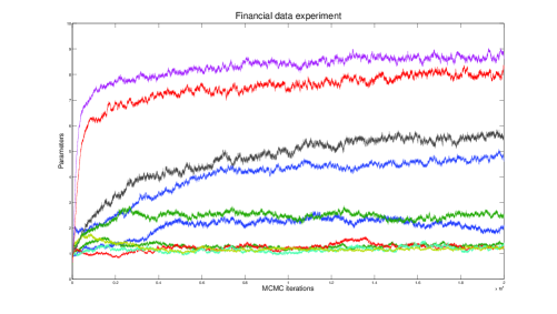
Figure 3: MCMC traces of the 10 parameters for the 46 log-returns data. Convergence is slow, although each step is relatively cheap.

The stocks are partitioned into 4 clusters according to the main category of business of the respective companies, with cluster sizes varying from 6 to 15. We define a CDF field using 10 factors: one for each cluster, and one for each pair of clusters using a Clayton copula for each factor. This is not a sparse model in terms of independences among the observed $\{U_{1},\dots,U_{46}\}$. However, in the corresponding latent DAG model there are only 10 latent variables with each observation $U_{i}$ having only two parents.

We used a Metropolis-Hastings method where each $\theta_{i}$ is sampled in turn conditioning on all other parameters using slice sampling [18]. Latent variables are sampled one by one using a simple random walk proposal. A gamma $(2,2)$ prior is assigned to each copula parameter independently. Figure 3 illustrates the trace obtained by initializing all parameters to 1. Although each iteration is relatively cheap, convergence is substantially slow, suggesting that latent variables and parameters have a strong dependence in the posterior. As is, the approach does not look particularly practical. Better proposals than random walks are necessary, with slice sampling each latent variable being far too expensive and not really addressing the posterior dependence between latent variables and parameters.

Our second experiment is a simple illustration of the proposed methods for a sparse model. Sparse models can be particularly useful to model residual dependence structure, as in the structural equation examples of [23]. Here we use synthetic data on a simple chain $U_{1}\leftrightarrow\dots\leftrightarrow U_{5}$ using all three approaches: one where we collapse the latent variables and perform MCMC moves using only the observed likelihood calculated by dynamic programming; another where we sample the four continuous latent variables explicitly (the “continuous latent” approach); and the third, where we simply treat our differential indicators as discrete latent variables (the “discrete latent” approach). Clayton copulas with gamma $(2,2)$ priors were again used, and exponents $a_{ij}$ were once again fixed uniformly. As before, slice sampling was used for the parameters, but not for the continuous latent variables.

Figure 4 summarizes the result of a synthetic study with a random choice of parameter values and a chain of five variables (a total of 4 parameters). For the collapsed and discrete latent methods, we ran the chain for 1000 iterations, while we ran the continuous latent method for 10000 iterations with no sign of convergence. The continuous latent method had a computational cost of about three to four times less than the other two methods. Surprisingly, the collapsed and discrete latent methods terminated in roughly the same amount of wallclock time, but in general we expect the collapsed sampler to be considerably more expensive. The effective sample size for the collapsed method along the four parameters was $(1000,891,1000,903)$ and for the discrete latent case we obtained $(243,151,201,359)$.

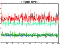
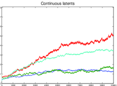
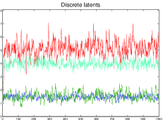
Figure 4: Sampling performance for the synthetic case study using the three different methods.

6 Discussion

Cumulative distribution fields provide another construction for copula functions. They are particularly suitable for sparse models where many marginal independences are expected, or for conditional models (as in [23]) where residual association after accounting for major factors is again sparsely located. We did not, however, consider the problem of identifying which sparse structures should be used, and focused instead on computing the posterior distribution of the parameters for a fixed structure.

The failure of the continuous latent representation as auxiliary variables in a MCMC sampler was unexpected. We conjecture that more sophisticated proposals than our plain random walk proposals should make a substantial difference. However, the main advantage of the continuous latent representation is for problems with large factors and a small number of factors compared to the number of variables. In such a situation perhaps the product of CDFs formulation should not be used anyway, and practitioners should resort to it for sparse problems. In this case, both the collapsed and the discrete latent representations seem to offer a considerable advantage over models with explicit latent variable representations (at least computationally), a result that was already observed for a similar class of independence models in the more specific case of Gaussian distributions [24].

An approach not explored here was the pseudo-marginal method [1], were an in place of the intractable likelihood function we use a positive unbiased estimator. In principle, the latent variable formulations allow for that. However, in a preliminary experiment where we used the very naive uniform distribution as an importance distribution for the discrete variables $\mathbf{Z}$, in a 10-dimensional chain problem with 100 data points, the method failed spectacularly. That is, the chain hardly ever moved. Far more sophisticated importance distributions will be necessary here.

Expectation-propagation (EP) [16] approaches can in principle be developed as alternatives. A particular interesting feature of this problem is that marginal CDFs can be read off easily, and as such energy functions for generalized EP can be derived in terms of actual marginals of the model.

For problems with discrete variables, the approach can be used almost as is by introducing another set of latent variables, similarly to what is done in probit models. In the case where dynamic programming by itself is possible, a modification of (1) using differences instead of differentiation leads to a similar discrete latent variable formulation (see the Appendix of [22]) without the need of any further set of latent variables. However, the corresponding function is not a joint distribution over $\mathbf{Z}\cup\mathbf{U}$ anymore, since differences can generate negative numbers.

Some characterization of the representational power of products of copulas was provided by [14], but more work can be done and we also conjecture that the point of view provided by the continuous latent variable representation described here can aid in understanding the constraints entailed by the cumulative distribution field construction.

References

- [1] Andrieu, C., Roberts, G.: The pseudo-marginal approach for efficient Monte Carlo computations. The Annals of Statistics 37, 697––725 (2009)
- [2] Bedford, T., Cooke, R.: Vines: a new graphical model for dependent random variables. Annals of Statistics 30, 1031–1068 (2002)
- [3] Cowell, R., Dawid, A., Lauritzen, S., Spiegelhalter, D.: Probabilistic Networks and Expert Systems. Springer-Verlag (1999)
- [4] Drton, M., Richardson, T.: A new algorithm for maximum likelihood estimation in Gaussian models for marginal independence. Proceedings of the 19th Conference on Uncertainty in Artificial Intelligence (2003)
- [5] Drton, M., Richardson, T.: Binary models for marginal independence. Journal of the Royal Statistical Society, Series B 70, 287–309 (2008)
- [6] Elidan, G.: Copulas in Machine Learning. Lecture Notes in Statistics (to appear)
- [7] Hofert, M.: Sampling Archimedean copulas. Computational Statistics & Data Analysis 52, 5163––5174 (2008)
- [8] Huang, J., Frey, B.: Cumulative distribution networks and the derivative-sum-product algorithm. Proceedings of the 24th Conference on Uncertainty in Artificial Intelligence (2008)
- [9] Huang, J., Frey, B.: Cumulative distribution networks and the derivative-sum-product algorithm: Models and inference for cumulative distribution functions on graphs. Journal of Machine Learning Research 12, 301–348 (2011)
- [10] Huang, J., Jojic, N., Meek, C.: Exact inference and learning for cumulative distribution functions on loopy graphs. Advances in Neural Information Processing Systems 23, 874–882 (2010)
- [11] Joe, H.: Multivariate Models and Dependence Concepts. Chapman-Hall (1997)
- [12] Kirshner, S.: Learning with tree-averaged densities and distributions. Neural Information Processing Systems (2007)
- [13] Kschischang, F., Frey, B., Brendan, J., Loeliger, H.A.: Factor graphs and the sum-product algorithm. IEEE Transactions on Information Theory 47, 498––519 (2001)
- [14] Liebscher, E.: Construction of asymmetric multivariate copulas. Journal of Multivariate Analysis 99, 2234–2250 (2008)
- [15] Marshall, A., Olkin, I.: Families of multivariate distributions. Journal of the American Statistical Association 83, 834–841 (1988)
- [16] Minka, T.: Automatic choice of dimensionality for PCA. Advances in Neural Information Processing Systems 13, 598–604 (2000)
- [17] Murray, I., Ghahramani, Z., MacKay, D.: MCMC for doubly-intractable distributions. Proceedings of 22nd Conference on Uncertainty in Artificial Intelligence (2006)
- [18] Neal, R.: Slice sampling. The Annals of Statistics 31, 705–767 (2003)
- [19] Nelsen, R.: An Introduction to Copulas. Springer-Verlag (2007)
- [20] Pearl, J.: Probabilistic Reasoning in Expert Systems: Networks of Plausible Inference. Morgan Kaufmann (1988)
- [21] Richardson, T., Spirtes, P.: Ancestral graph Markov models. Annals of Statistics 30, 962–1030 (2002)
- [22] Silva, R.: Latent composite likelihood learning for the structured canonical correlation model. Proceedings of the 28th Conference on Uncertainty in Artificial Intelligence, UAI (2012)
- [23] Silva, R.: A MCMC approach for learning the structure of Gaussian acyclic directed mixed graphs. In: P. Giudici, S. Ingrassia, M. Vichi (eds.) Statistical Models for Data Analysis, pp. 343–352. Springer (2013)
- [24] Silva, R., Ghahramani, Z.: The hidden life of latent variables: Bayesian learning with mixed graph models. Journal of Machine Learning Research 10, 1187–1238 (2009)
- [25] Walker, S.: Posterior sampling when the normalising constant is unknown. Communications in Statistics - Simulation and Computation 40, 784––792 (2011)