Forcing homogeneous turbulence in DNS of particulate flow with interface resolution and gravity

Abstract

We consider the case of finite-size spherical particles which are settling under gravity in a homogeneous turbulent background flow. Turbulence is forced with the aid of the random forcing method of Eswaran and Pope [Comput. Fluids, 16(3):257-278, 1988], while the solid particles are represented with an immersed-boundary method. The forcing scheme is used to generate isotropic turbulence in vertically elongated boxes in order to warrant better decorrelation of the Lagrangian signals in the direction of gravity. Since only a limited number of Fourier modes are forced, it is possible to evaluate the forcing field directly in physical space, thereby avoiding full-size transforms. The budget of box-averaged kinetic energy is derived from the forced momentum equations. Medium-sized simulations for dilute suspensions at low Taylor-scale Reynolds number $Re_{\lambda}=65$, small density ratio $\rho_{p}/\rho_{f}=1.5$ and for two Galileo numbers $Ga=0$ and $120$ are carried out over long time intervals in order to exclude the possibility of slow divergence. It is shown that the results at zero gravity are fully consistent with previous experimental measurements and available numerical reference data. Specific features of the finite-gravity case are discussed with respect to a reduction of the average settling velocity, the acceleration statistics and the Lagrangian auto-correlations.

I Introduction

Particulate flow is a rich scientific topic which bears a multitude of open questions, some of which have broad practical consequences. One example is the settling speed of heavy solid particles which are suspended in a fluid undergoing turbulent motion. Predicting its average value and higher statistical moments is certainly of great interest in fields such as meteorology and chemical engineering. However, our current knowledge of the underlying dynamical processes in particulate flow systems is still incomplete, to a large extent due to a lack of detailed data covering the entire multi-parameter space. As a consequence the predictive capabilities of existing engineering-type models are still relatively limited.

Interface-resolved direct numerical simulation (DNS) of idealized particulate flows is starting to become a viable option for generating high-fidelity data-sets complementing data obtained through laboratory measurements. Most numerical studies in this spirit have either focused upon plane channel flow^{1, 2, 3, 4, 5} or upon homogeneous-isotropic turbulence^{6, 7, 8, 9, 10}. In homogeneous flows without mean deformation, a turbulent background field is typically either obtained through a suitably chosen initial condition with a subsequent energy decay^{9, 10}, or the turbulent fluctuations are generated by explicitly adding an energy input to the Navier-Stokes equations^{6, 7, 8}. The latter approach has the obvious advantage of allowing for a statistically-stationary state to be reached and maintained as long as desired, thereby facilitating the simulation of processes occurring on a long time-scale, such as particle cluster formation¹¹.

Most turbulence forcing methods are formulated in Fourier space, and the energy input is restricted to the largest scales, i.e. to low wavenumbers^{12, 13, 14, 15}. One notable exception is the forcing scheme proposed by Lundgren¹⁶ (cf. also Ref.17), in which an additional forcing term directly proportional to the velocity vector itself is added to the momentum equation. While in most approaches the momentum forcing mechanism indeed depends upon the state of the flow field (deterministic forcing), the methods proposed by Eswaran and Pope¹⁸ and by Alvelius¹⁹ construct the forcing term randomly in a manner which is independent of the flow field.

In simulations of particulate flow with fully-resolved phase-interfaces there are several additional points to be considered when choosing a turbulence forcing scheme. First, it should be recalled that the particle motion is naturally two-way coupled to the fluid flow, which means that the question of numerical stability of the discretized Navier-Stokes equations involving a turbulent forcing scheme arises. Second, in the presence of inertial particles and non-zero gravity, the particle phase experiences a mean gravitational acceleration, which in turn through the mean drag provides a source term to the fluid’s kinetic energy equation. As a consequence, the coupled system’s kinetic energy budget is significantly modified as compared to the zero-gravity (or neutrally-buoyant) case. Finally, it should be kept in mind that the numerical requirements for fully-resolved particulate flow can be substantially harder to meet than for single-phase turbulence. This is particularly true for the case with finite gravity, since mean particle settling places additional requirements upon the small-scale resolution and upon the computational domain size in the vertical direction.

Therefore, in the present context we require the following properties of a turbulence forcing method:

1. In single-phase flow it should allow for simulations which yield small-scale statistics in agreement with previous studies.

2. It should allow for stable long-time integration in the presence of particles which are fully two-way coupled to the flow field, even in the presence of finite gravity.

3. It should be efficient to compute in the framework of a numerical method which is not based upon Fourier transform (i.e. not pseudo-spectral).

4. It should allow for a reasonable a priori estimation of the parameter values which need to be set in order to attain the target values of the turbulence scales.

A number of forcing schemes which have been proposed in the past do not fulfill the entire set of the above requirements. In particular, the linear forcing method of Lundgren^{16, 17} – although very attractive in view of requirement (III) – does not fulfill requirement (II), as already noted by Naso and Prosperetti²⁰. Our own experience confirms this observation: applying Lundgren’s linear forcing to two-way coupled particulate flow problems leads to unbounded growth of the kinetic energy (Doychev and Uhlmann, unpublished results).

Forcing schemes which potentially seem to adapt to all of the above requirements are those which are based upon external random processes^{18, 19}. In this category the force term which is added to the momentum equation does not depend upon the velocity field itself, therefore eliminating a source of instability when applied to particulate flow.

The first numerical study of forced homogeneous-isotropic turbulence seeded with finite-size resolved particles has been performed by Ten Cate et al.⁶ who employed a lattice-Boltzmann method and maintained statistically stationary turbulence with the aid of Alvelius’ random forcing scheme¹⁹. These authors pre-computed a number of realizations of the forcing field and imposed it in a random sequence upon the flow field. Homann and Bec⁷ used a Fourier pseudo-spectral Navier-Stokes solver in conjunction with a penalty method to represent individual finite-size particles, while keeping the energy content of two small-wavenumber shells constant. Yeo et al.⁸ represented the action of finite-size particles upon the flow by means of the force-coupling method of Lomholt and Maxey²¹; in their simulations turbulence was maintained statistically stationary with the random forcing method of Eswaran and Pope¹⁸. In all of these studies^{6, 7, 8} the particles’ submerged weight was zero (either because of a density ratio of unity or because of zero gravity). Therefore, the problems and open questions associated with mean particle settling in a turbulent environment still remain largely unsolved.

The aim of the present paper is to discuss the feasibility of investigating with fully-resolved simulations the motion of particles which are larger than the Kolmogorov scale, have a higher density than the fluid, and which are subjected to finite gravity. The random forcing scheme of Eswaran and Pope¹⁸ is employed to generate a turbulent background field, and the immersed-boundary technique of Uhlmann²² is used to force the no-slip condition at the interface between the fluid and the solid particles. The purpose of the present contribution is two-fold. On the one hand we present the methodology of turbulence forcing in the framework of two-way particulate flow with gravity. A study of this configuration, for which case several adaptations of the basic forcing method are necessary, has to our knowledge not been published to the present date. We feel that it is important to ensure that the chosen forcing strategy satisfies the four requirements set forth above, in particular regarding numerical stability. Here we apply the turbulence forcing scheme to obtain isotropic turbulence in vertically-elongated boxes; with a slight modification this method allows us to simulate heavy particles which settle with respect to the forcing field. On the other hand the evolution of the kinetic energy in this system which exhibits two source terms (related to gravity and to large-scale forcing) has not been investigated in detail. Here we analyze the energy budget derived from the momentum equation solved in the simulations, which includes two volume force terms (the large-scale turbulence forcing and the forcing of the no-slip interface condition). Results are presented from medium-sized simulations of dilute suspensions at low turbulent Reynolds number and intermediate Galileo number. Where possible the present results are compared to available experimental and numerical reference data from previous studies.

II Numerical method

We present in this section the numerical method as well as the main statistical quantities considered in this study. The equations which describe the motion of an incompressible fluid with constant density $\rho_{f}$ and constant kinematic viscosity $\nu$ can be written as follows

$$\frac{\partial\mathbf{u}}{\partial t}+(\mathbf{u}\cdot\nabla)\mathbf{u}+\frac{1}{\rho_{f}}\nabla p = \nu\nabla^{2}\mathbf{u}+{\bm{\mathcal{F}}}\,,$$ (1a)

$$\nabla\cdot\mathbf{u} = 0\,,$$ (1b)

where $\mathbf{u}$ denotes the fluid velocity vector and $p$ the hydrodynamic pressure. The vector ${\bm{\mathcal{F}}}$ (which will be further specified below) collects all specific volume force terms associated with: (a) generating and maintaining homogeneous turbulence (denoted as $\mathbf{f}^{(t)}$ in the following), and (b) the representation of the solid particles ($\mathbf{f}^{(p)}$) in the framework of an immersed boundary technique. Therefore, the total volume force term in the most general case considered here is given by the sum of these two contributions:

$${\bm{\mathcal{F}}}=\mathbf{f}^{(t)}+\mathbf{f}^{(p)}\,.$$ (2)

II.1 Forcing homogeneous-isotropic turbulence

We consider a forcing method which is expressed as a momentum source term $\mathbf{f}^{(t)}(\mathbf{x},t)$ introduced into (1a) through (2). The formulation is based upon random processes driving the time evolution of a number of large scales (i.e. small wavenumber Fourier modes). Two variants of this category of forcing methods have been proposed and employed by various authors in the past: the scheme of Eswaran & Pope¹⁸ (henceforth denoted as “EP”) and the scheme by Alvelius¹⁹. The principle difference between these two approaches lies in the characteristic time-scale over which the random processes are correlated: in EP an explicit forcing time-scale can be prescribed, whereas Alvelius’ method does not involve such time-scale (i.e. the random processes are uncorrelated from step to step). In the present work we have chosen EP’s method, since it allows us to investigate the influence of the forcing time scale. If required, essentially uncorrelated random processes can be recovered by choosing the forcing time-scale equal to the numerical time step, as will be made more precise below.

We summarize below the main characteristics of EP forcing; for more details we refer the reader to the original work¹⁸. The EP forcing method is first formulated in Fourier space. Let $\bm{\kappa}=(\kappa_{1},\kappa_{2},\kappa_{3})$ denote the wavenumber vector which can be defined in a cuboidal domain with side-lengths $({\cal L}_{x},{\cal L}_{y},{\cal L}_{z})$ in the three physical space directions. The forcing term in Fourier space is denoted by $\hat{\mathbf{f}}^{(t)}(\bm{\kappa},t)$. It is non-zero only in a low-wavenumber band for which $|\bm{\kappa}|\leq\kappa_{f}$, where $\kappa_{f}$ is a parameter to be determined. Note that the origin $\bm{\kappa}=0$ is not forced. The vector of complex Fourier coefficients $\hat{\mathbf{f}}^{(t)}(\bm{\kappa},t)$ is computed from six independent Uhlenbeck-Ornstein processes (the real and imaginary parts of each one of the three vector components) for each of the forced wavenumbers. The components of the complex vector describing the random process, denoted as $\hat{\mathbf{b}}(\bm{\kappa},t)$, are given by the following finite-difference equation:

$$\hat{b}_{i}(\bm{\kappa},t+\Delta t)=\hat{b}_{i}(\bm{\kappa},t)\left(1-\frac{\Delta t}{T_{L}}\right)+e_{i}(\bm{\kappa},t)\left(2\sigma^{2}\frac{\Delta t}{T_{L}}\right)^{1/2}\,,\quad\forall\,\,i=1,2,3\,.$$ (3)

In (3) the symbol $\Delta t$ denotes the numerical time step, $e_{i}(\bm{\kappa},t)$ is a complex random number drawn (at each time step and for each wavenumber) from a standardized Gaussian distribution (with zero mean and variance unity), $T_{L}$ is the characteristic time scale of the random process, and $\sigma^{2}$ its variance. It can be seen that choosing $T_{L}=\Delta t$ corresponds to a random process which is uncorrelated in time. As shown by EP, in the limit as $\Delta t$ tends to zero the process (3) has zero mean ($\langle\hat{\mathbf{b}}(\bm{\kappa},t)\rangle=0$, the angular brackets indicating statistical averaging), and its temporal correlation indeed exhibits an exponential decay, viz.

$$\langle\hat{b_{i}}(\bm{\kappa},t)\hat{b_{j}}^{*}(\bm{\kappa},t+s)\rangle=2\sigma^{2}\delta_{ij}\exp(-s/T_{L})\,,$$ (4)

where an asterisk denotes complex conjugation.

The volume force term $\hat{\mathbf{f}}^{(t)}(\bm{\kappa},t)$ is obtained by orthogonal projection of the vector describing the random processes,

$$\hat{\mathbf{f}}^{(t)}(\bm{\kappa},t+\Delta t)=\hat{\mathbf{b}}(\bm{\kappa},t+\Delta t)-\bm{\kappa}(\bm{\kappa}\cdot\hat{\mathbf{b}}(\bm{\kappa},t+\Delta t))/(\bm{\kappa}\cdot\bm{\kappa})\,,$$ (5)

thereby guaranteeing zero divergence.

It can be seen that a total of three parameters are introduced by the EP scheme: $T_{L}$, $\kappa_{f}$ and $\sigma$. In practice the amplitude parameter $\sigma$ is not directly prescribed; instead a value for the combined quantity $\epsilon^{\ast}=\sigma^{2}\,T_{L}$ is imposed. Doing so (i.e. choosing the values for $T_{L}$ and $\epsilon^{\ast}$ independently) ensures that in the limit of vanishing $T_{L}$ the mean energy input does not trivially tend to zero¹⁸.

Since our Navier-Stokes solver is based upon finite differences, the Fourier series involving the coefficients given by (5) needs to be evaluated at the discrete grid points in physical space in order to determine the force field $\mathbf{f}^{(t)}(\mathbf{x},t)$. In order to avoid the cost associated with a complete fast Fourier transform step (which for massively parallel computations mainly stems from the necessary communication overhead), we perform a direct evaluation of the Fourier series. Note that when splitting up the transform into three successive one-dimensional transforms, this operation is computationally not expensive, as described in appendix A. Since each parallel process simulates the entire set of random processes redundantly in local memory, this procedure does not involve any inter-processor communication. Furthermore, since the number of forced Fourier modes (controlled by the parameter $\kappa_{f}$) is typically small (below $100$) the computational cost due to the turbulence forcing scheme remains small compared to the overall cost of a Navier-Stokes time-step. In practice we have observed an increase in the necessary wall-clock time per time step of roughly 10-15% for the cases considered in this work.

II.2 Representing particles with an immersed boundary method

The numerical method employed in the present simulations has been described in detail in Ref. 22. It has been previously used for the direct numerical simulation of various particulate flow configurations ³, ²³, ⁴, ²⁴, ²⁵, ²⁶, ¹¹, ²⁷, ²⁸.

The incompressible Navier-Stokes equations are solved by a fractional step approach with an implicit treatment of the viscous terms (Crank-Nicolson) and a low-storage, three-step Runge-Kutta scheme for the non-linear terms. The spatial discretization employs second-order central finite-differences on a staggered mesh which is uniform and isotropic (i.e. $\Delta x=\Delta y=\Delta z=cst.$).

The no-slip condition at the surface of moving solid particles is imposed by means of the specifically designed immersed boundary technique of Uhlmann²². This gives rise to an additional volume force term in the momentum equation which we denote as $\mathbf{f}^{(ibm)}$ (defined in appendix B). The appendix also gives the details of the presently chosen temporal integration of the Navier-Stokes equations in the presence of solid particles and artificial turbulence forcing. Furthermore, in order to be able to obtain a statistically stationary state when simulating settling bodies in a triply-periodic domain, it is necessary to compensate the average force exerted by the particles upon the fluid^{29, 30} (cf. appendix B). As a consequence, the particle-related contribution to the volume force field (2) which is added to the right-hand-side of the momentum equation (1a) reads:

$$\mathbf{f}^{(p)}(\mathbf{x},t)=\mathbf{f}^{(ibm)}(\mathbf{x},t)-\langle\mathbf{f}^{(ibm)}\rangle_{\Omega}(t)\,,$$ (6)

where $\langle\,\rangle_{\Omega}$ indicates an average over the entire computational domain comprising the fluid and the solid phase (cf. definition in appendix C).

On the other hand, the motion of the particles is computed from the Newton equations for linear and angular motion of rigid bodies, driven by buoyancy, hydrodynamic force/torque and contact forces (in case of collisions). Since the particle suspensions under consideration here are dilute, collisions are occurring infrequently. Therefore, in the present work they are treated by a simple repulsive force mechanism ³¹ formulated such as to keep colliding particles from overlapping non-physically. In the case of dense particle arrangements, the discrete element method of Ref. 27 can be employed instead.

II.3 The basic kinetic energy balance

Defining the instantaneous kinetic energy $E_{k}(\mathbf{x},t)=\mathbf{u}\cdot\mathbf{u}/2$, we can derive its transport equation from the momentum equation (1a). Substituting (2) and (6), and integrating the result over a triply-periodic spatial domain $\Omega$ yields the following evolution equation:

$$\frac{\mbox{d}}{\mbox{d}t}\langle E_{k}\rangle_{\Omega}=-\varepsilon_{\Omega}+\Psi^{(t)}+\Psi^{(p)}\,,$$ (7)

where we have defined the instantaneous box-averaged dissipation rate $\varepsilon_{\Omega}$, viz.

$$\varepsilon_{\Omega}(t)=2\nu\langle S_{ij}S_{ij}\rangle_{\Omega}\,,$$ (8)

with $S_{ij}=(u_{i,j}+u_{j,i})/2$, the work done by the turbulence forcing, $\Psi^{(t)}$,

$$\Psi^{(t)}(t)=\langle\mathbf{u}\cdot\mathbf{f}^{(t)}\rangle_{\Omega}\,,$$ (9)

as well as the fluid-particle coupling term, $\Psi^{(p)}$,

$$\Psi^{(p)}(t)=\langle\mathbf{u}\cdot\mathbf{f}^{(ibm)}\rangle_{\Omega}-\langle\mathbf{u}\rangle_{\Omega}\cdot\langle\mathbf{f}^{(ibm)}\rangle_{\Omega}\,.$$ (10)

The fluid-particle coupling term can be brought into a physically more insightful form by making use of the Newton-Euler equations for rigid body motion. This reformulation will be deferred until section IV.2 below.

Let us now define some further quantities which will be used in the following. The fluid phase velocity is decomposed into an average (over the region filled with fluid) and a fluctuation, viz.

$$\mathbf{u}(\mathbf{x},t)=\langle\mathbf{u}\rangle_{\Omega_{f}}(t)+\mathbf{u}^{\prime}(\mathbf{x},t)\,,$$ (11)

where the averaging operator $\langle\cdot\rangle_{\Omega_{f}}$ is defined in appendix C. Then the kinetic energy of the fluctuations, averaged over the fluid phase, is defined as

$$k(t)=\frac{1}{2}\langle\mathbf{u}^{\prime}\cdot\mathbf{u}^{\prime}\rangle_{\Omega_{f}}=\frac{3}{2}\,u_{rms}^{2}(t)\,,$$ (12)

where the characteristic velocity scale $u_{rms}(t)$ has been defined simultaneously. We also define a dissipation rate averaged over the fluid phase, viz.

$$\varepsilon(t)=2\nu\langle S_{ij}^{\prime}S_{ij}^{\prime}\rangle_{\Omega_{f}}\,.$$ (13)

From these quantities we can compute the Kolmogorov length scale $\eta=(\nu^{3}/\varepsilon)^{1/4}$, the Taylor micro-scale $\lambda=(15\nu u_{rms}^{2}/\varepsilon)^{1/2}$, the large-eddy length-scale $L=k^{3/2}/\varepsilon$, the large-eddy turn-over time $T_{e}=u_{rms}^{2}/\varepsilon$, the Kolmogorov time $\tau_{\eta}=(\nu/\varepsilon)^{1/2}$ and the vorticity fluctuation amplitude $\omega_{rms}=(\varepsilon/\nu)^{1/2}$.

III Simulation of single-phase turbulence

The aim of the present section is to provide a validation of the EP forcing technique in a finite-difference context, and to discuss its application to elongated computational domains.

III.1 Parameters, setup and flow characterization

The single-phase simulations were run with the numerical parameters specified in table 1. Let us first focus on cases A and B which feature cubic domains with $256^{3}$ and $512^{3}$ grid nodes, respectively (the cases AL, BL featuring elongated boxes will be discussed in § III.2 below). The forcing parameters $\kappa_{f}$, $T_{L}$, and $\varepsilon^{*}$ are chosen such that a very good small-scale resolution $\eta/\Delta x$ can be obtained, while a reasonable ratio between the box-size ${\cal L}_{x}$ and the integral length scale can be maintained (in the worst case this ratio is approximately equal to $7$). With the given moderate number of grid points, the target Reynolds number $Re_{\lambda}=\lambda u_{rms}/\nu$ (based upon the Taylor micro-scale $\lambda$) is approximately 60 and 140, respectively. The procedure for choosing the forcing parameters which yield the target Reynolds number and small-scale resolution is specified in appendix D.

Some simulations were first started on a coarser grid in order to speed up the computation during the initial transient. They were subsequently interpolated onto the final grid, and the simulations were continued. Averages have been computed (on the finest grid) in the statistically stationary regime over intervals larger than $25$ large-eddy time scales ($T_{e}$), cf. Table 2. The table also shows the obtained Reynolds number, length scales, the non-dimensional dissipation rate as well as the skewness of the velocity gradients derived from these statistical results.

case	$\Omega=\mathcal{L}_{x}\times\mathcal{L}_{y}\times\mathcal{L}_{z}$	$N_{x}\times N_{y}\times N_{z}$	$\kappa_{f}/\kappa_{x,1}$	$N_{F}$	$T_{L}\nu/{\cal L}_{x}^{2}$	$\varepsilon^{*}{\cal L}_{x}^{4}/\nu^{3}$
A	$\mathcal{L}_{x}=\mathcal{L}_{y}=\mathcal{L}_{z}$	$256^{3}$	$2.3$	$56$	$2.12\cdot 10^{-4}$	$3.72\cdot 10^{7}$
B	$\mathcal{L}_{x}=\mathcal{L}_{y}=\mathcal{L}_{z}$	$512^{3}$	$2.5$	$80$	$5.94\cdot 10^{-5}$	$3.52\cdot 10^{9}$
AL	$\mathcal{L}_{x}=\mathcal{L}_{y}=\mathcal{L}_{z}/2$	$256^{2}\times 512$	$2.3$	$56$	$2.12\cdot 10^{-4}$	$3.72\cdot 10^{7}$
BL	$\mathcal{L}_{x}=\mathcal{L}_{y}=\mathcal{L}_{z}/2$	$512^{2}\times 1024$	$2.5$	$80$	$5.94\cdot 10^{-5}$	$3.52\cdot 10^{9}$

Table 1: Imposed parameters in the present single-phase simulations. The size of the computational domain $\Omega$ is given in terms of its linear dimensions ${\cal L}_{x}$, ${\cal L}_{y}$, ${\cal L}_{z}$. The number of grid points along the coordinate directions are denoted by $N_{x}$, $N_{y}$, $N_{z}$. The forcing cut-off wavenumber $\kappa_{f}$ is normalized by the smallest wavenumber in the $x$-coordinate direction ($\kappa_{x,1}$); $N_{F}$ denotes the total number of Fourier modes which are forced.

case	$Re_{\lambda}$	$L/{\cal L}_{x}$	$\lambda/{\cal L}_{x}$	$\eta/{\cal L}_{x}$	$\eta/\Delta x$	$T_{e}\omega_{rms}$	$\varepsilon L_{f}/u_{rms}^{3}$	$S(u_{,x})$	$T_{obs}/T_{e}$
A	$65.5$	$0.5970$	$0.0744$	$4.673\cdot 10^{-3}$	$1.20$	$16.92$	$1.3378$	$-0.5109$	$79.7$
B	$143.0$	$0.5665$	$0.0323$	$1.374\cdot 10^{-3}$	$0.704$	$37.26$	$1.2971$	$-0.5341$	$80.5$
AL	$65.0$	$0.5934$	$0.0743$	$4.678\cdot 10^{-3}$	$1.20$	$16.93$	$1.3461$	$-0.5064$	$33.9$
BL	$141.6$	$0.5604$	$0.0323$	$1.379\cdot 10^{-3}$	$0.706$	$36.57$	$1.3114$	$-0.5341$	$60.8$

Table 2: Physical parameters of the present single-phase simulations. $L=k^{3/2}/\varepsilon$ denotes the large-eddy length scale, $\lambda=(15\nu u_{rms}^{2}/\varepsilon)^{1/2}$ is the Taylor micro-scale with $Re_{\lambda}=\lambda u_{rms}/\nu$ the corresponding Reynolds number, $\eta=(\nu^{3}/\varepsilon)^{1/4}$ the Kolmogorov length scale, $\Delta x$ the grid width, $T_{e}=u_{rms}^{2}/\varepsilon$ the large-eddy turn-over time, $L_{f}=2\pi/\kappa_{f}$ the forcing length scale, $S(u_{,x})$ the skewness of the velocity derivatives and $T_{obs}$ is the total simulated time. The vorticity fluctuation amplitude $\omega_{rms}=(\varepsilon/\nu)^{1/2}$ has been used as a time-scale for the normalization of $T_{e}$. All quantities were evaluated from time-averages after the statistically stationary regime was reached in the respective simulation.

The time evolution of box-averaged fluctuation energy $k$ and dissipation rate $\varepsilon$ as well as the Reynolds number $Re_{\lambda}$ is shown in figure 1. Therein we use the forcing parameters $T_{L}$ and $\varepsilon_{T}^{\ast}$ (cf. appendix D) to construct reference values for the fluctuation energy, $k_{ref}=3T_{L}\varepsilon_{T}^{\ast}/2$, and for the dissipation rate, $\varepsilon_{ref}=\varepsilon_{T}^{\ast}$. It can be observed that a statistically stationary state is reached after roughly $6T_{e}$ during which the energy cascade is forming. For later times the flow state oscillates around well-defined time-averages for each quantity.

$(a)$

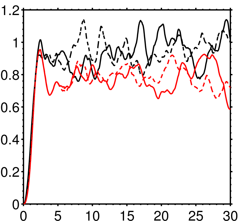
$t/T_{e}$

$k/k_{ref}$

$\varepsilon/\varepsilon_{ref}$

$(b)$

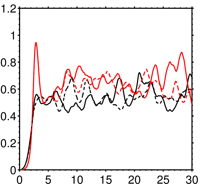
$t/T_{e}$

$(c)$

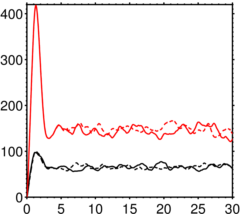
$t/T_{e}$

$Re_{\lambda}$

Figure 1: Temporal evolution of box-averaged quantities: $(a)$ kinetic energy of the fluctuations, $(b)$ dissipation rate, $(c)$ Reynolds number. The lines styles correspond to:   case A,   case B,       case AL,       case BL. The definition of the reference scales $k_{ref}$ and $\varepsilon_{ref}$ is given in the text. Note that only a sub-set of the simulated time interval is shown for clarity.

Figure 2 additionally shows for case B the only two source terms of the kinetic energy budget (7) which are non-zero in the single-phase context. It can be seen that the energy input $\Psi^{(t)}$ is oscillating on a scale which corresponds to the imposed parameter value $T_{L}$ ($T_{L}/T_{e}=0.84$ in case B). The dissipation rate data exhibit a smoother temporal evolution, with an overall similar shape as the power input, albeit with a certain time-lag.

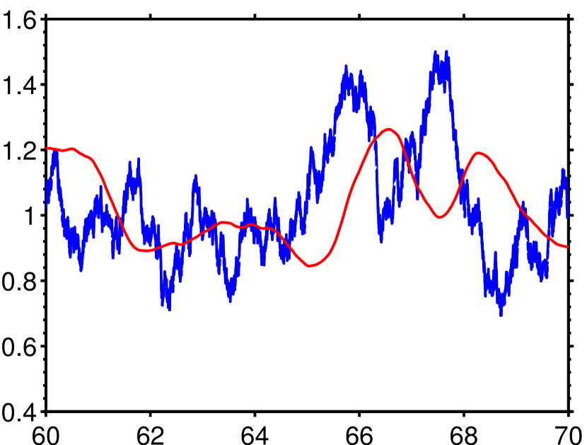
$t/T_{e}$

$\varepsilon/\langle\varepsilon\rangle_{t}$, $\Psi^{(t)}/\langle\varepsilon\rangle_{t}$

Figure 2: Time evolution of volume-averaged viscous dissipation $\varepsilon$ ( ) and of turbulence forcing power input $\Psi^{(t)}$ ( ) in case B, both scaled by the time-average value of the dissipation rate $\langle\varepsilon\rangle_{t}$. Note that an arbitrarily chosen time interval in the statistically stationary regime is shown.

Snapshots of the modulus of vorticity in a slice through the computational domain are shown in figure 3, where the typical intermittent multi-scale patterns featuring various size eddies as well as very thin filaments can be distinguished.

$(a)$

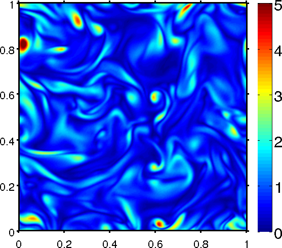
$x/{\cal L}_{x}$

$z/{\cal L}_{x}$

$z/{\cal L}_{x}$

$(b)$

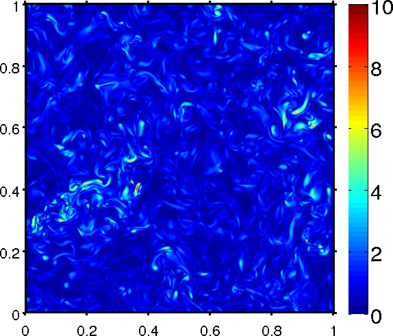
$x/{\cal L}_{x}$

$(c)$

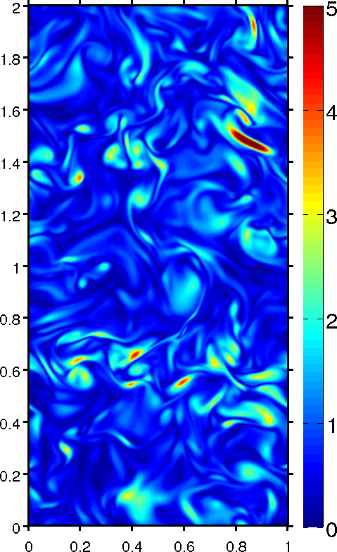
$x/{\cal L}_{x}$

$z/{\cal L}_{x}$

$z/{\cal L}_{x}$

$(d)$

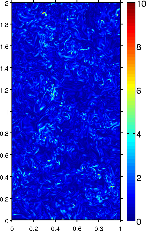
$x/{\cal L}_{x}$

Figure 3: Snapshots of the modulus of vorticity normalized by $\omega_{rms}$, shown in one plane. $(a)$ case A, $(b)$ case B, $(c)$ case AL, $(d)$ case BL.

Let us proceed to a quantitative comparison with respect to reference data of Jiménez et al.¹² (also available in electronic form in Ref.32) which were obtained through DNS with the aid of a pseudo-spectral method. Those authors assured energy input to the large scales through a negative viscosity in a small-wavenumber band; the amplitude was dynamically adjusted such as to maintain the small-scale resolution constant. Their series of simulations covers the present range of parameters, with two simulations featuring nearly identical Reynolds number values as presently simulated ($Re_{\lambda}=62$ and $142$). Figure 4 shows the probability density (p.d.f.) of longitudinal and transverse velocity gradients. It can be seen that the statistics of the present simulations closely match the data of Ref.12 all the way down to extreme events with six orders of magnitude smaller probability than the maximum. Note that the p.d.f. of the velocity flucutations themselves (cf. appendix E) exhibits the well known Gaussian behavior.

$(a)$

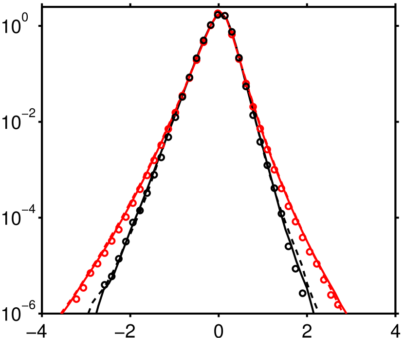
$(\partial u_{\alpha}/\partial x_{\alpha})/\omega_{rms}$

pdf

pdf

$(b)$

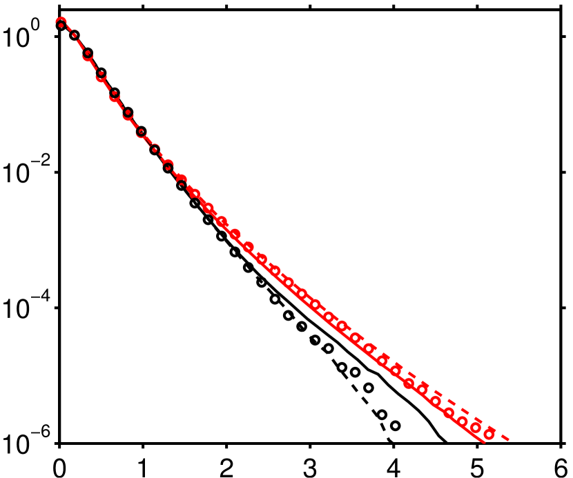
$(\partial u_{\alpha}/\partial x_{\beta})/\omega_{rms}$

Figure 4: Normalized probability density functions of velocity gradients: $(a)$ longitudinal gradients, $(b)$ transverse gradients. The lines and symbols correspond to:   case A;       case AL;   case B;       case BL; ‘$\bm{\circ}$’ Jiménez et al.¹², $Re_{\lambda}=62$; ‘$\bm{\circ}$’ Jiménez et al.¹², $Re_{\lambda}=142$.

The time-averaged energy spectra are shown in figure 5 and 6. Both three-dimensional and one-dimensional spectra practically collapse with the data of Jiménez et al.¹² at the corresponding Reynolds number. Only slight differences can be discerned at the smallest wavenumbers, as can be expected in view of the different forcing methods employed. It should be remarked that the small-scale resolution employed here (in terms of $\eta/\Delta x$, cf. table 2) is very good compared to studies which employed similar second-order, finite-difference based discretization of the Navier-Stokes equations¹⁰.

$(a)$

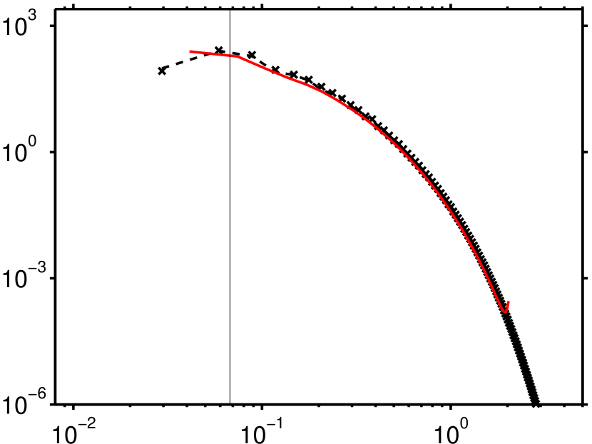
$\kappa\,\eta$

$E(\kappa)/(\varepsilon^{2/3}\eta^{5/3})$

$E(\kappa)/(\varepsilon^{2/3}\eta^{5/3})$

$(b)$

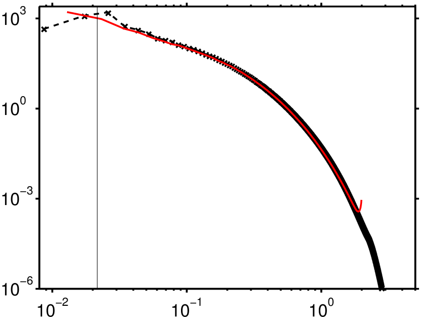
$\kappa\,\eta$

Figure 5: Three-dimensional energy spectra computed from at least 10 flow fields in the observation interval. Data at $Re_{\lambda}\approx 60$ are shown in $(a)$:      , case A, ${{\times}}$, case AL. The graph in $(b)$ collects the data at $Re_{\lambda}\approx 140$:      , case B, ${{\times}}$, case BL. The solid lines ( ) correspond to the reference data of Jiménez et al.¹² at $Re_{\lambda}=62$ and at $Re_{\lambda}=142$, respectively. The thin vertical lines indicate the respective cut-off wavenumber of the turbulence forcing scheme, $\kappa_{f}$.

$(a)$

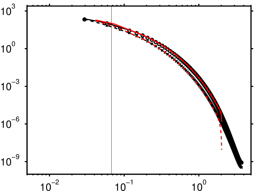
$\kappa_{\beta}\,\eta$

$E_{\alpha\alpha}(\kappa_{\beta})/(\varepsilon^{2/3}\eta^{5/3})$

$E_{\alpha\alpha}(\kappa_{\beta})/(\varepsilon^{2/3}\eta^{5/3})$

$(b)$

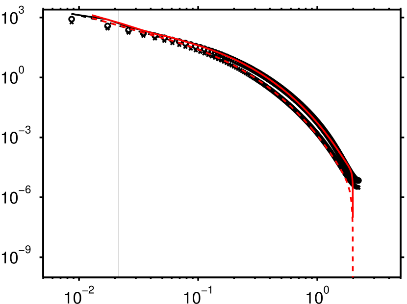
$\kappa_{\beta}\,\eta$

Figure 6: One-dimensional energy spectra. Data at $Re_{\lambda}\approx 60$ are shown in $(a)$:      , case A longitudinal,  , case A transverse, ${{\times}}$, case AL longitudinal, ${{{\circ}}}$, case AL transverse,      , Jiménez et al.¹² longitudinal,  , Jiménez et al.¹² transverse. The graph in $(b)$ collects the data at $Re_{\lambda}\approx 140$:      , case B longitudinal,  , case B transverse, ${{\times}}$, case BL longitudinal, ${{{\circ}}}$, case BL transverse,      , Jiménez et al.¹² longitudinal,  , Jiménez et al.¹² transverse. The thin vertical lines indicate the respective cut-off wavenumber of the turbulence forcing scheme, $\kappa_{f}$.

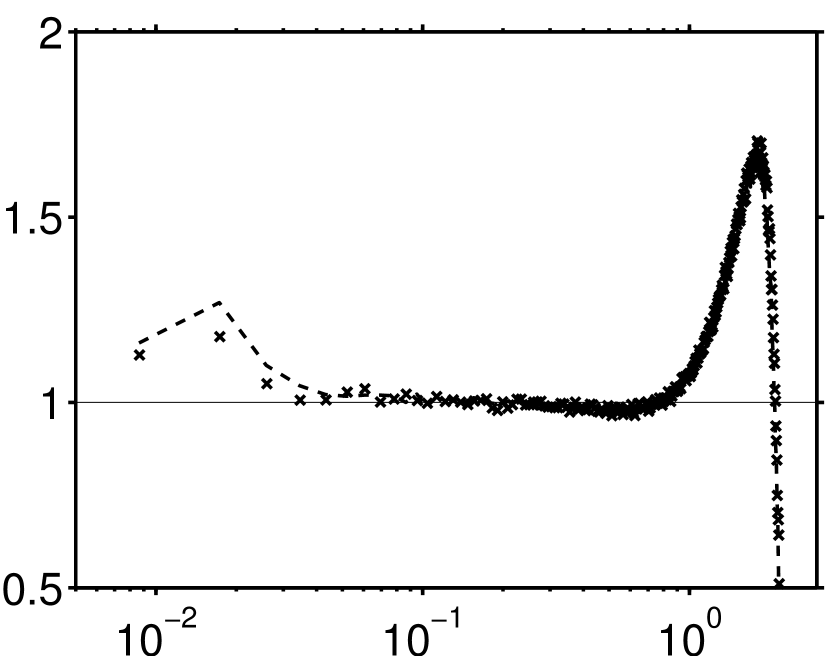
$\kappa_{1}\,\eta$

$I(\kappa_{1})$

Figure 7: The isotropy parameter $I$ defined in (15) as a function of the wavenumber $\kappa_{1}$, shown for case B (     ) and BL ($\bm{\times}$).

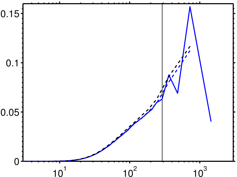
$\lambda_{\alpha}/\eta$

$\kappa_{\alpha}E_{\alpha\alpha}(\kappa_{\alpha})/(\varepsilon^{2/3}\eta)$

$R_{ww}$

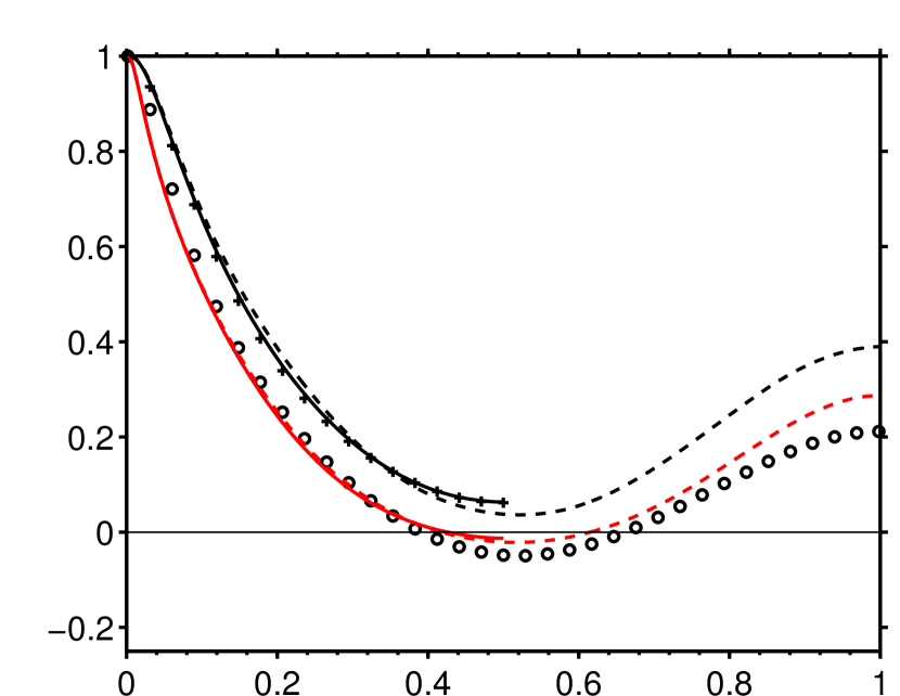
$r_{z}/{\cal L}_{x}$

Figure 8: $(a)$ Premultiplied longitudinal energy spectrum at $Re_{\lambda}\approx 140$, similar to some of the information in figure 6$(b)$.       case B;       case BL, short sides ($\alpha=1,2$);   case BL, elongated side ($\alpha=3$). Note that the horizontal axis shows the wavenumber $\lambda_{\alpha}=2\pi/\kappa_{\alpha}$. The thin vertical line delimits the wavelength corresponding to the forcing cut-off $\kappa_{f}$. $(b)$ Longitudinal two-point correlation function in the $z$-coordinate direction, $R_{ww}(r_{z})$. The lines correspond to:   case A;       case AL;   case B;       case BL. The two particulate flow cases of section IV are indicated by the following symbols: ‘$\bm{+}$’ case A-G0; ‘$\bm{\circ}$’ case AL-G120.

III.2 Isotropic turbulence in elongated boxes

In the case of gravity-induced particle settling in a vertically-periodic computational domain unphysical results may be caused by the two following situations: (i) particles encounter their own wakes after performing one trip around the vertical box-size (${\cal L}_{z}$), and/or (ii) particles interact with the same flow structures after one vertical round-trip. Situation (i) occurs if the vertical domain size is smaller than the axial distance after which the velocity deficit in the wake has decayed to a negligible amplitude. In some sense the case of sedimenting particles without background turbulence¹¹ is the “worst case”, since the decay of the velocity deficit is accelerated by the presence of background turbulence^{33, 34, 35, 36, 4}. Situation (ii) occurs when the particle return time (defined as the vertical domain size divided by the average settling velocity) is smaller than the largest life-time of all turbulent eddies. Fede et al.³⁷ recommend that the particle return time should be four times larger than the integral time scale in order to avoid statistical bias of Lagrangian particle data caused by vertical periodicity.

Therefore, in the case of two-phase flow with settling particles it is generally desirable to employ computational domains that are sufficiently long in the vertical direction. In practice this requirement leads to the use of non-cubic domains which are elongated in the direction of gravity. At the same time it is desirable to maintain the spatial isotropy of the forced turbulence. Note that we refer here to the isotropy of the turbulent flow field in the absence of settling particles, since the effect of particle settling will immediately break the statistical symmetry.

In order to achieve an approximately statistically isotropic flow, we have formulated the forcing term $\hat{\mathbf{f}}^{(t)}(\bm{\kappa})$ in a perfectly isotropic manner. This is automatically assured in the case that the side-lengths of the cuboidal domain in physical space, $({\cal L}_{x},{\cal L}_{y},{\cal L}_{z})$, are integer multiples of one of them (here arbitrarily taken as ${\cal L}_{x}$), viz. ${\cal L}_{y}=n{\cal L}_{x}$, and ${\cal L}_{z}=m{\cal L}_{x}$. If the definition of the discrete wavenumbers appearing in the forcing scheme (as defined in equation 23) is simply replaced by the following one

$$\kappa_{\alpha,i}^{(iso)}=\frac{2\pi i}{{\cal L}_{x}}\,,\quad\forall\,\,i=-N_{f}\ldots N_{f}\,,$$ (14)

the forcing term $\hat{\mathbf{f}}^{(t)}$ defined in (3-5) is statistically isotropic.

In order to verify whether the resulting flow field remains isotropic in case of a non-cubic computational box, we have performed additional simulations with twice elongated boxes in the $z$-coordinate direction (i.e. $n=1$, $m=2$) while maintaining the grid width $\Delta x=\Delta y=\Delta z$. These cases are denoted as “AL” and “BL”, where all other parameters remain unchanged with respect to the corresponding simulations in cubic boxes (cf. table 1). Note that elongation of the domain has introduced new Fourier modes into the system, but due to (14) we do not force them. As can be seen from table 2 we do not observe a statistically significant influence of this elongation on the resulting flow scales. The time evolution of energy and dissipation, as well as flow visualization and pdfs (cf. figures 1-4) all confirm that we essentially obtain the same flow irrespective of the elongation of the domain.

A more stringent test of isotropy can be performed by considering the isotropy parameter $I$ introduced in Ref.12, viz.

$$I(\kappa_{1})=\frac{E_{11}(\kappa_{1})-\kappa_{1}\,\partial E_{11}(\kappa_{1})/\partial\kappa_{1}}{2E_{22}(\kappa_{1})}\,,$$ (15)

which is equal to unity for all wavenumbers $\kappa_{1}$ in the case of a strictly homogeneous-isotropic velocity field (Ref.38, p. 50). From figure 7 it can be seen that there exists indeed a considerable range of wavenumbers over which the flow can be judged as isotropic. As in previous studies (e.g. Ref.12) this excludes the largest scales (those which are directly forced); likewise, the smallest scales start to deviate from the isotropic value for $\kappa_{1}\eta\geq 1$.

We now turn to the effect of elongating the box in the $z$-direction upon the energy spectra. Figure 8$(a)$ shows the longitudinal one-dimensional energy spectrum in case BL, where the average of the data along the short directions ($E_{11}(\kappa_{1})$, $E_{22}(\kappa_{2})$) is compared to the corresponding spectrum along the elongated direction, i.e. $E_{33}(\kappa_{3})$. Note that the data are presented in form of premultiplied spectra as function of the wavelength $\lambda_{\alpha}=2\pi/\kappa_{\alpha}$ in order to facilitate the discussion. It can be seen that the spectral energy density along short directions is practically identical to the corresponding spectrum evaluated in the cubical box in case B. The counterpart represented along the elongated direction ($\alpha=3$), on the other hand, exhibits an alternating behavior in the range of wavelengths larger than the forcing cut-off $\lambda>2\pi/\kappa_{f}$: those modes which directly receive power input from the forcing scheme have a larger energy content than in the cubical case, and those which are interspersed (i.e. the unforced modes) have a significantly smaller amplitude. The implications of the large-scale energy distribution for the flow field in elongated boxes are best discussed in terms of two-point correlations. Figure 8$(b)$ shows the longitudinal correlation function in the $z$-coordinate direction, $R_{ww}(r_{z})$. In the cases with cubic domains we obtain an approximate decorrelation at the maximum separation (equal to half the box size, $r_{z}/{\cal L}_{x}=0.5$), with the correlation values $R_{ww}(r_{z}/{\cal L}_{x}=0.5)=0.06$ and $-0.01$ in cases A and B, respectively. In the cases with a twice elongated domain the longitudinal correlation functions in the direction of elongation are practically identical to the corresponding cubical cases up to $r_{z}/{\cal L}_{x}=0.5$, and then they increase monotonically up to $0.39$ ($0.29$) at separations equal to half the elongated side length in case AL (BL). This means that the flow field in adjacent cubical sub-domains retains a non-negligible correlation – a consequence of the fact that the forcing is applied only to every $n$th Fourier mode in a direction which is elongated by an integer factor $n$ Note that an exact $n$-fold copy of a given cubical domain would result in the two-point correlation $R_{ww}(r_{z})$ to be exactly symmetric with respect to the point $r_{z}={\cal L}_{x}/n$, i.e. it would increase again up to the value of unity at a separation of $r_{z}/{\cal L}_{x}=1$. Therefore, elongating the computational domain in a simulation of single-phase isotropic turbulence does not promise any substantial benefit. In the two-phase case with settling particles, however, it is still a useful technique in view of the two situations which can cause a non-physical bias of the Lagrangian particle statistics mentioned at the beginning of the present section. This is because the particle positions themselves will not present any periodicity other than the fundamental one. Therefore, their wakes tend to be less correlated over the elongated domain size and the particles’ effect upon the flow field (two-way coupling) will tend to reduce the observed correlation of the single-phase case. Figure 8$(b)$ indeed confirms this for the particulate flow case AL-G120 with finite settling velocity which will be discussed in detail in section IV. It can be seen that the correlation value at the largest separation is decreased by 46% with respect to case AL, yielding $R_{ww}(r_{z}/{\cal L}_{x}=1)=0.21$. Note that in the particulate flow cases the velocity field was first continued inside the space occupied by the particles by means of linear interpolation involving only grid nodes located inside the fluid; then, as in the single-phase cases, the two-point correlation functions were computed with the aid of Fourier transform.

IV Simulation of forced turbulence in the presence of finite-size particles

In the previous section it was shown that basic tests with single-phase flow provide good agreement with the literature, and elongating the computational domain in one direction appears to be an option for the case with settling particles. We also verified that the forcing method considered here satisfies points I, III and IV of the requirements set forth in the introduction, and we now apply this forcing scheme to the case of particle-laden flows in order to ensure that requirement II is also satisfied, and that statistics are in agreement with data from the literature in the two-phase case.

For this purpose we are considering the flow in a triply-periodic domain seeded with $N_{p}$ solid, spherical particles of equal diameter $D$ and density $\rho_{p}$. The system experiences a constant gravitational acceleration $\mathbf{g}$ which is directed into the negative $z$-coordinate direction. Simultaneously, the random forcing procedure described above is used in order to generate additional turbulent fluctuations.

IV.1 Parameters of the problem and setup of the simulations

Whereas in the single-phase counterpart a single dimensionless group (i.e. a Reynolds number such as $Re_{\lambda}$) adequately describes the system, dimensional analysis shows that the multi-particle case requires five such parameters. The additional four non-dimensional parameters can be taken as the following ones: the solid volume fraction $\phi_{s}=N_{p}V_{p}/({\cal L}_{x}{\cal L}_{y}{\cal L}_{z})$ (where $V_{p}=\pi D^{3}/6$ is the volume occupied by a single particle); the density ratio $\rho_{p}/\rho_{f}$; the length scale ratio $D/\eta$; the Galileo number $Ga=u_{g}D/\nu$, where a gravitational velocity is defined as $u_{g}=(|\rho_{p}/\rho_{f}-1||\mathbf{g}|D)^{1/2}$.

case	$\phi_{s}$	$\rho_{p}/\rho_{f}$	$Ga$	$D/\eta$	$D/\Delta x$	$\mathcal{L}_{x}\times\mathcal{L}_{y}\times\mathcal{L}_{z}$	$N_{p}$	$Nx\times N_{y}\times N_{z}$	$T_{obs}/T_{e}$
A-G0	$0.005$	$1.5$	$0$	$6.7$	16	$32D\times 32D\times 32D$	$313$	$512^{3}$	$49.7$
AL-G120	$0.005$	$1.5$	$120$	$6.7$	16	$32D\times 32D\times 64D$	$616$	$512^{2}\times 1024$	$27.6$

Table 3: Imposed parameters in the particle-laden simulations. Note that in both cases the turbulence forcing parameters are identical to the single-phase case A (cf. Table 2). For the purpose of normalization in this table the time-averaged values of $\eta$ and $T_{e}$ in the single-phase simulation are used.

case	$Re_{\tilde{\lambda}}=\tilde{\lambda}u_{rms}/\nu$	$I=u_{rms}/w_{rel}$	$\langle Re_{p}\rangle_{t}=|\langle w_{rel}\rangle_{t}|D/\nu$
A-G0	$65.4$	–	–
AL-G120	$66.2$	$0.197$	$137.6$

Table 4: Some additional physical parameters of the particle-laden simulations. All quantities were evaluated from time-averages after the statistically stationary regime was reached in the respective simulation.

Two cases are considered, with and without gravity, under otherwise identical conditions. For this purpose we have chosen the turbulence forcing parameters of cases A and AL of section III which (in the absence of particles) yield a moderate Reynolds number of $Re_{\lambda}=65$ in both cases (cf. tables 1 and 2), the only difference being the vertical domain size. Here we use the cubical domain of the single-phase case A for the simulation of a zero-gravity particle-laden case which we denote as case A-G0; likewise we use the vertically elongated domain of single-phase case AL in a particle-laden case with the Galileo number set to $120$, henceforth denoted as case AL-G120. An isolated heavy particle at the latter Galileo number ($Ga=120$, for any density ratio $\rho_{p}/\rho_{f}>1$) settles steadily on a vertical path, featuring an axisymmetric wake^{39, 26}. The remaining imposed non-dimensional parameters are identical in both particulate cases (cf. Table 3): the suspension can be considered as dilute with a solid volume fraction $\phi_{s}=0.005$, while the density ratio is set to $\rho_{p}/\rho_{f}=1.5$ (which corresponds e.g. to some plastic materials such as PVC in water), and the particle diameter is larger than (but comparable to) the Kolmogorov length scale, $D/\eta=6.7$; note that this value as well as the following length scale ratios are based upon the average dissipation rate $\langle\varepsilon\rangle_{t}$ obtained in the corresponding single-phase simulations. In both cases A-G0 and AL-G120 the particle diameter corresponds to $0.42$ Taylor length scales and to $0.05$ large eddy length scales. It is known that in the absence of turbulence the dilute suspension with the parameter set ($\phi_{s}=0.005$, $\rho_{p}/\rho_{f}=1.5$, $Ga=120$) as chosen in the present case AL-G120 does not form significant wake-induced particle clusters¹¹.

In the particulate flow problem a number of additional time scales can be defined. First, the particle response time (based upon Stokes drag) is given by $\tau_{p}=D^{2}\rho_{p}/(18\nu\rho_{f})$. In the case of finite gravity, a gravitational time scale can be inferred from the gravitational velocity $u_{g}$ and the particle diameter, viz. $\tau_{g}=D/u_{g}$. In the simulations A-G0 and AL-G120 the ratio between the Stokes drag time scale and the Kolmogorov time (i.e. the typical small-scale Stokes number) is larger than unity ($\tau_{p}/\tau_{\eta}=3.73$), where the time-scale of the flow is based upon single-phase data from case A (cf. table 2); the Stokes number is smaller than unity when based upon the integral time scale ($\tau_{p}/T_{e}=0.22$). Therefore, we can expect the particles to respond at least partially to the hydrodynamic forces caused by the turbulent background flow. In the finite gravity case AL-G120 the gravitational (settling) time scale is less than half as large as the Kolmogorov time ($\tau_{g}/\tau_{\eta}=0.37$, again based upon single-phase data). At the same time the standard deviation of the turbulent background velocity field (measured in the absence of particles) is nearly five times smaller than the gravitational velocity scale ($u_{rms}/u_{g}=0.22$). This indicates that the vertical velocity will be the dominant contribution to the particle motion, but that the influence of turbulence will not be negligibly small. Flow visualisation (such as shown in figure 9) indeed demonstrates the effect of gravity, i.e. the formation of significant vorticity in the wakes of the settling particles.

$(a)$

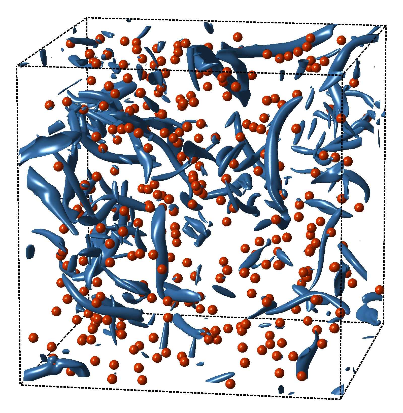
$(b)$

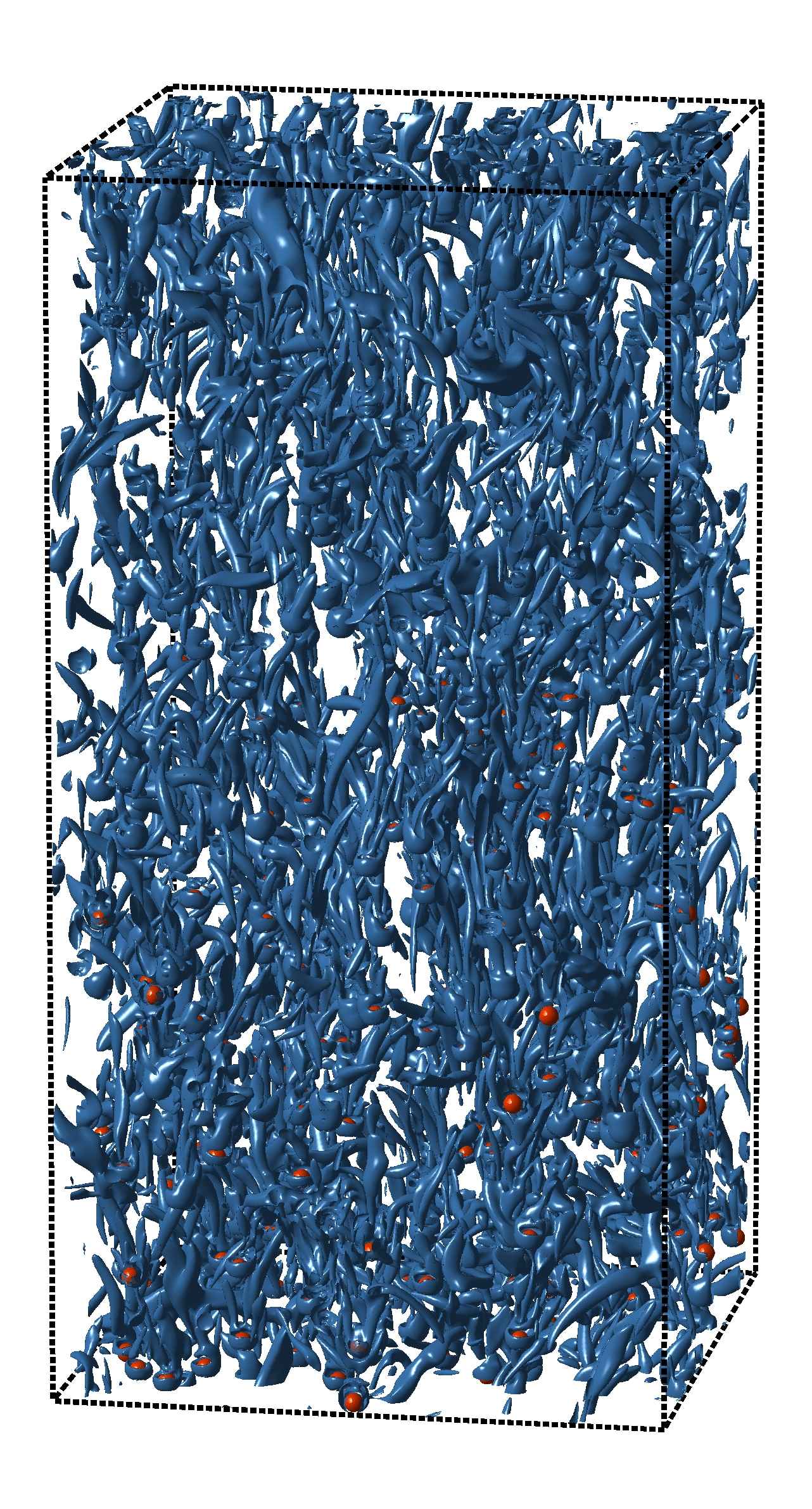
Figure 9: Visualization of instantaneous vortical structures identified with the q-criterion of Hunt et al.⁴⁰ (blue iso-surfaces, $q/\omega_{rms}^{2}=1$, where $\omega_{rms}$ is taken from single-phase flow) and particle positions (red spheres): $(a)$ case A-G0; $(b)$ case AL-G120.

The start-up of the present simulations is again performed in a step-wise manner. First, the grid of the single-phase cases A and AL is used in cases A-G0 and AL-G120, respectively, and a developed single-phase flow field is used as initial condition, while particles are added at random positions. The particles are first held fixed in space. After several integral time scales have elapsed, the grid is refined (by linear interpolation) to its final resolution of $D/\Delta x=16$ (cf. validation in Refs.26, 11), and the simulation is further advanced for several integral time scales (the particles still being fixed in space). Finally, particles are released with an initial velocity equal to zero. We arbitrarily set the time to zero at the moment of release.

In the finite-gravity case AL-G120 a constant (positive) vertical velocity $w_{sh}$ was added to the initial flow field taken from the single-phase simulation case AL (at time $t=t_{sh}$), in order to impose a mean relative velocity while particles are initially held fixed with respect to the computational grid. The value of $w_{sh}$ was determined from the anticipated settling velocity of an isolated sphere¹¹. Since the turbulent background flow in this case is effectively transported with velocity $\mathbf{u}_{sh}=(0,0,w_{sh})$, we apply a phase-shift to the forcing term by a corresponding amount, i.e. we modify $\hat{\mathbf{f}}^{(t)}$ given in (5) by the following expression:

$$\hat{\mathbf{f}}_{sh}^{(t)}(\bm{\kappa},t)=\hat{\mathbf{f}}^{(t)}(\bm{\kappa},t)\,\exp(-I(t-t_{sh})\bm{\kappa}\cdot\mathbf{u}_{sh})\,,$$ (16)

(where $I=(-1)^{1/2}$), then replace $\hat{\mathbf{f}}^{(t)}$ in (2) by $\hat{\mathbf{f}}_{sh}^{(t)}$.

IV.2 Temporal evolution and the kinetic energy budget

$(a)$

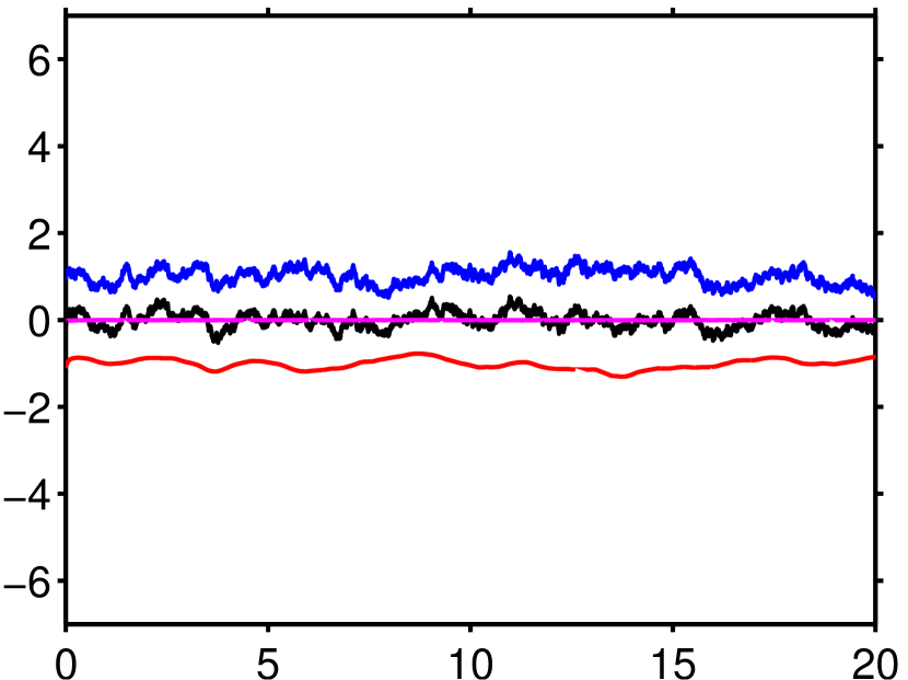
$t/T_{e}$

budget

budget

$(b)$

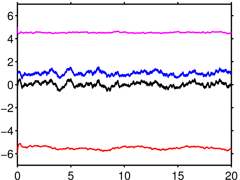
$t/T_{e}$

Figure 10: Time evolution of the terms in the budget of volume-averaged kinetic energy (7): $(a)$ case A-G0, $(b)$ case AL-G120. Line styles:  , turbulence forcing ($\Psi^{(t)}$);  , fluid-particle coupling ($\Psi^{(p)}$);  , dissipation ($-\varepsilon_{\Omega}$);  , time rate-of-change ($-\mbox{d}\langle E_{k}\rangle_{\Omega}/\mbox{d}t$). All terms are normalized by the time-average value of the dissipation rate in the corresponding single-phase case.

The temporal evolution of the four individual terms of the box-averaged kinetic energy equation (7) are shown in figure 10. Recall that in the particulate case the time-rate-of-change of $\langle E_{k}\rangle_{\Omega}$ is the result of a balance between turbulence-forcing power input ($\Psi^{(t)}$), dissipation rate ($\varepsilon_{\Omega}$) and fluid-particle coupling term ($\Psi^{(p)}$). The figure shows that in the zero-gravity case the fluid-particle coupling term is negligibly small (its time-average is equal to $0.002$ times the mean single-phase dissipation rate value), and that both the magnitude of the dissipation rate and that of the turbulence forcing power input are of similar values as the single-phase counterparts in case A which features the same external turbulence forcing parameters (the relative differences of the time-averaged values amount to 2% and 3.5%, respectively). This result might actually be expected on the grounds of the small solid volume fraction and the absence of average relative velocity. In fact, in the simulations with decaying homogeneous-isotropic turbulence performed by Lucci et al.^{10, 41} the two particle sets with the smallest volume fraction (cases “B” in Ref.10 and Ref.41, both at $\phi_{s}\approx 0.01$ and $\rho_{p}/\rho_{f}\approx 2.5$) exhibit a similarly small effect upon the temporal evolution of the turbulent kinetic energy and upon the dissipation rate as observed in the present case A-G0.

Concerning the finite-gravity case AL-G120, we observe in figure 10$(b)$ that while the magnitude of the power input due to turbulence forcing is similar to the single-phase counterpart, the fluid-particle coupling term now dominates the balance, while the magnitude of the dissipation is likewise increased by nearly a factor of six. It can be seen that the kinetic energy budget is fundamentally different in the case with non-zero gravity even at a relatively small solid volume fraction, mainly due to the increased dissipation in the wakes.

Let us mention that the box-averaged kinetic energy balance (7) is fulfilled by the simulation data up to the contribution due to numerical error. In the present case A-G0 (AL-G120) the maximum residual amounts to $0.005$ ($0.059$) times the time average of the dissipation rate ($\langle\varepsilon_{\Omega}\rangle_{t}$). Grid refinement by a factor $3/2$ in case AL-G120 leads to a reduction of the maximum residual to a value of $0.032\langle\varepsilon_{\Omega}\rangle_{t}$. The fulfillment of the numerically evaluated kinetic energy balance can therefore be considered as an additional grid convergence test which to our knowledge has previously not been reported in interface-resolved particulate flow simulations.

In order to further elucidate the kinetic energy budget, we rewrite the fluid-particle coupling term in (10) through use of the Newton-Euler equation for rigid body motion of spherical particles as follows:

$$\Psi^{(p)}(t)=\phi_{s}\left(\frac{\rho_{p}}{\rho_{f}}-1\right)\mathbf{u}_{rel,\Omega}\cdot\mathbf{g}+\Psi^{(p)}_{accel}(t)+\Psi^{(p)}_{coll}(t)\,,$$ (17)

where the contributions due to particle acceleration ($\Psi^{(p)}_{accel}$) and due to inter-particle collisions ($\Psi^{(p)}_{coll}$) are defined in appendix F. Furthermore, an apparent slip velocity with respect to the box-averaged velocity, defined as $\mathbf{u}_{rel,\Omega}=\langle\mathbf{u}_{p}^{(i)}\rangle_{p}-\langle\mathbf{u}\rangle_{\Omega}$, has been used in setting up (17). Since the two-way coupling term is negligibly small in the zero-gravity case A-G0, we now focus on case AL-G120. The data in the latter case show that the sum of the particle acceleration and particle collision terms ($\Psi^{(p)}_{accel}+\Psi^{(p)}_{coll}$) is negligibly small compared to the gravity term in (17). Substituting (17) into (7), performing statistical averaging (or time averaging over a statistically stationary interval) and neglecting the small terms then yields the following approximate relation:

$$\tilde{\varepsilon}\equiv\langle\varepsilon_{\Omega}\rangle_{t}-\phi_{s}\left(\frac{\rho_{p}}{\rho_{f}}-1\right)\langle\mathbf{u}_{rel,\Omega}\rangle_{t}\cdot\mathbf{g}\approx\langle\Psi^{(t)}\rangle_{t}\,.$$ (18)

From this balance it can be argued that the difference between the mean dissipation rate and the gravity term, which we henceforth denote as $\tilde{\varepsilon}$, represents the dissipation rate of the “background” turbulence. In other words this amounts to removing the added dissipation of the work done by the gravitational potential. We will use the quantity $\tilde{\varepsilon}$ in the definition of a modified Taylor micro-scale

$$\tilde{\lambda}=(15\nu u_{rms}^{2}/\tilde{\varepsilon})^{1/2}\,,$$ (19)

from which a modified Reynolds number $Re_{\tilde{\lambda}}=\tilde{\lambda}u_{rms}/\nu$ can be formed. Due to the anisotropy of the flow in the presence of gravity, the surrogate Taylor micro-scale in (19) does obviously not correspond to its original definition in homogeneous-isotropic turbulence (e.g. Ref.42). It is here simply used in order to provide a means of computing a value for the Reynolds number based on this length scale, as this is the most widely used one in homogeneous turbulence. Indeed, since the work done by the turbulence forcing is only little affected by the presence of the settling particles, the Reynolds number $Re_{\tilde{\lambda}}$ based upon the definition (19) is practically the same in case AL-G120 and in case A-G0 (cf. table 4), and the value closely matches the one of the corresponding single-phase cases (cf. table 2).

$(a)$

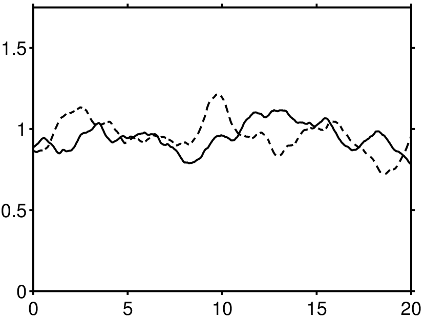
$t/T_{e}$

$k/k_{ref}$

$k_{p}/k_{ref}$

$(b)$

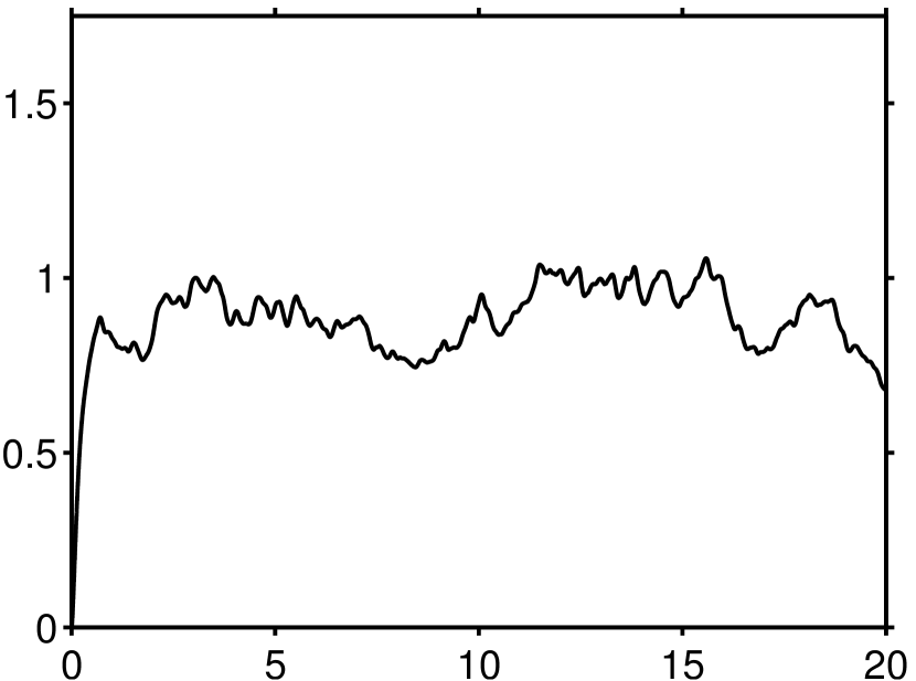
$t/T_{e}$

Figure 11: The energy associated with the velocity fluctuations of both phases in case A-G0: $(a)$ fluid phase turbulent kinetic energy $k$ defined in (12); $(b)$ solid phase kinetic energy of the fluctuations $k_{p}\equiv\langle\mathbf{u}_{p}^{\prime}\cdot\mathbf{u}_{p}^{\prime}\rangle_{p}/2$. The dashed line in $(a)$ corresponds to the evolution of $k$ in the single-phase case A. Note that only part of the simulated interval is shown for clarity.

$(a)$

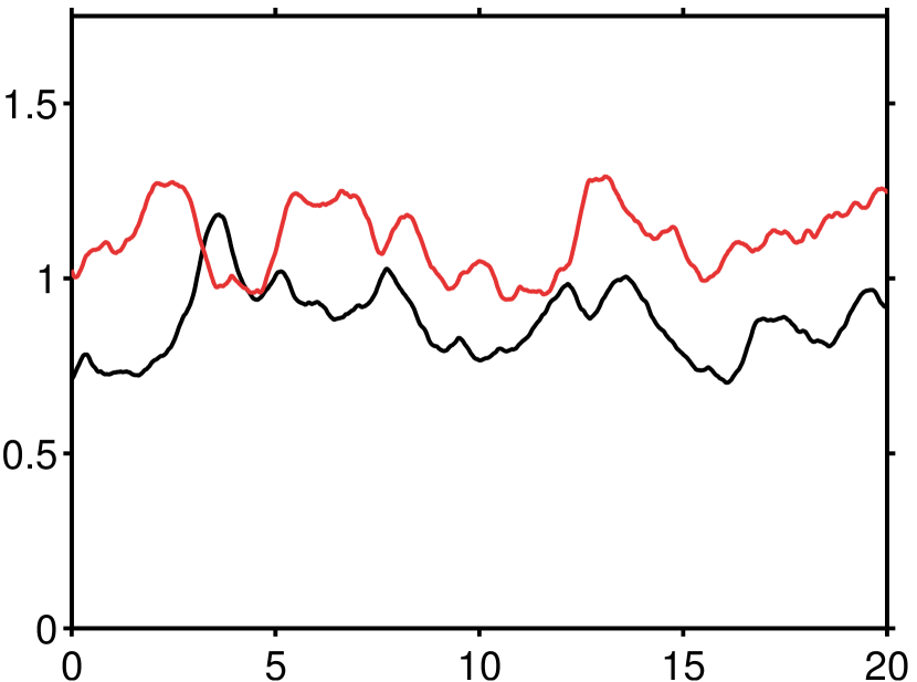
$t/T_{e}$

$k/k_{ref}$

$k_{p}/k_{ref}$

$(b)$

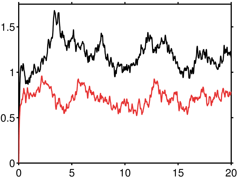
$t/T_{e}$

Figure 12: The energy associated with the velocity fluctuations of both phases in case AL-G120, distinguishing between the horizontal and vertical directions. $(a)$ fluid phase; $(b)$ solid phase. In $(a)$ the black solid line corresponds to the horizontal component $k^{(h)}\equiv 3(\langle u^{\prime}u^{\prime}\rangle_{\Omega_{f}}+\langle v^{\prime}v^{\prime}\rangle_{\Omega_{f}})/4$; the red solid line shows the vertical component $k^{(v)}\equiv 3\langle w^{\prime}w^{\prime}\rangle_{\Omega_{f}}/2$. Note that with this definition $k=(2k^{(h)}+k^{(v)})/3$, and that in particular for an ideally isotropic velocity field $k=k^{(h)}=k^{(v)}$ would hold. In $(b)$ the corresponding quantities $k_{p}^{(h)}$ and $k_{p}^{(v)}$ are plotted with the same line-styles as in $(a)$, where the fluid velocity fluctuations $\mathbf{u}^{\prime}$ are replaced by the particle velocity fluctuations $\mathbf{u}_{p}^{\prime}$, and the averaging is over the number of particles ($\langle\,\rangle_{p}$ instead of $\langle\,\rangle_{\Omega_{f}}$). The reference scale $k_{ref}$ is the same as in figure 1. Note that only part of the simulated interval is shown for clarity.

Next we examine the temporal evolution of the energy associated to fluctuations of the fluid velocity field and the particles. Figure 11 shows the turbulent kinetic energy of the fluid (defined in 12) in case A-G0 together with the same quantity in the single-phase case A. Both signals exhibit similar features concerning time scales and amplitude of the fluctuations, the time average of the particulate case A-G0 being 2.2% lower than the single-phase counterpart. Note that the amplitude of the temporal fluctuations of $k$ is less than 10% of its time-average value when using the present forcing scheme. The kinetic energy of the particulate phase, analogously defined as $k_{p}\equiv\langle\mathbf{u}_{p}^{\prime}\cdot\mathbf{u}_{p}^{\prime}\rangle_{p}/2$, quickly reaches a statistically stationary state after particle release in case A-G0; afterwards it fluctuates around a time-average which is approximately 6% lower than the fluid-phase kinetic energy. Furthermore, the two quantities $k_{p}$ and $k$ are clearly positively correlated in this case.

Turning now to the finite-gravity case AL-G120 (figure 12), we need to distinguish the vertical from the horizontal directions. For this purpose we separately define two kinetic energy contributions $k^{(v)}\equiv 3\langle w^{\prime}w^{\prime}\rangle_{\Omega_{f}}/2$ and $k^{(h)}\equiv 3(\langle u^{\prime}u^{\prime}\rangle_{\Omega_{f}}+\langle v^{\prime}v^{\prime}\rangle_{\Omega_{f}})/4$ which are constructed such that $k=(2k^{(h)}+k^{(v)})/3$, i.e. $k=k^{(h)}=k^{(v)}$ holds in case of isotropy. It can be observed from the figure that gravity indeed breaks the isotropy, with the vertical component fluctuating around a larger time-average value than the horizontal one (by 24%). This result can be explained by the fact that particle wakes predominantly constitute fluctuations of the vertical fluid velocity component. The particle kinetic energy contributions $k_{p}^{(v)}$ and $k_{p}^{(h)}$, which are analogously defined as $k^{(v)}$ and $k^{(h)}$ (cf. figure 12$b$), on the other hand, exhibit an inverse ordering, i.e. the horizontal component is larger than the vertical one (on average by 71%). This observation can be understood by recalling that the force fluctuations of fixed spheres either swept by homogeneous-isotropic turbulence⁴³ or towed through a homogeneous-isotropic turbulent flow field⁴⁴ exhibit the same anisotropy, i.e. the standard-deviation of the lateral force component is larger than the axial one. It can therefore be expected that in the case of mobile spheres the intensity of the lateral (horizontal) particle velocity generated by these force fluctuations is larger than the corresponding axial (vertical) one.

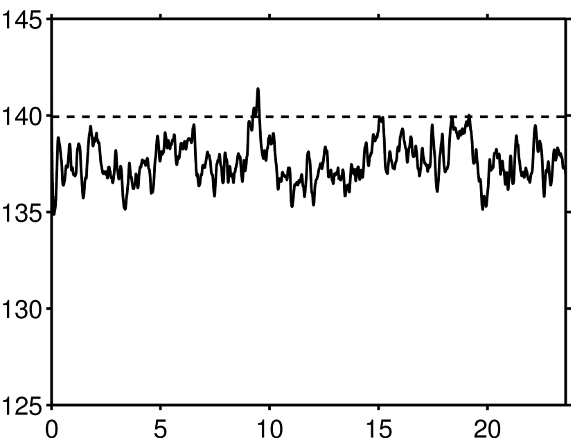
$t/T_{e}$

$Re_{p}$

Figure 13: Temporal evolution of the mean particle settling velocity normalized by viscous particle scales, $Re_{p}=|w_{rel}|D/\nu$ in case AL-G120. The dashed line corresponds to the value for an isolated sphere in ambient fluid, which was extrapolated from the simulation with $Ga=121.24$ in Ref.11, supposing that the ratio $|w_{rel}|/u_{g}$ remains constant.

A quantity of considerable interest for many applications is the average settling velocity of the particles with respect to the global average velocity of the fluid phase, viz.

$$\mathbf{u}_{rel}=\langle\mathbf{u}_{p}^{(i)}\rangle_{p}-\langle\mathbf{u}\rangle_{\Omega_{f}}\,.$$ (20)

Figure 13 shows the absolute value of the vertical component of (20) in viscous particle scaling, i.e. a settling Reynolds number $Re_{p}=|w_{rel}|D/\nu$, in the finite-gravity case AL-G120. The time-average of $Re_{p}$ measures $137.6$, which is approximately 1.5% smaller than the average settling Reynolds number of an isolated sphere in ambient fluid at the same Galileo number and density ratio (the reference value was extrapolated from the simulation “S121” with $Ga=121.24$ in Ref.11, supposing that the ratio $|w_{rel}|/u_{g}$ remains constant). Although collective effects cannot be ruled out, they appear unlikely at the present solid volume fraction and in the absence of any indication of particle clustering. Indeed Voronoï tesselation analysis shows that no significant departure from a random particle distribution is taking place in either flow case (cf. appendix G). Therefore, the likely cause for the slightly reduced average settling velocity lies in the turbulent background flow.

One model for understanding reduced particle settling in a turbulent environment is non-linear drag^{45, 43}: if one assumes that the instantaneous drag on the particle can be described by a non-linear function of some properly defined “velocity seen by the particle”, then any superposed fluctuations of this fluid velocity can lead to an increase of the mean particle drag force, even if the fluctuations are symmetrically distributed. Homann et al.⁴⁴ have shown that if one assumes an isolated sphere is swept by a velocity composed of a constant $w_{rel}$ plus a Gaussian random vector (whose components are independently and identically distributed with standard-deviation $u_{rms}$) and if a standard drag formula (Schiller-Naumann⁴⁶) is invoked instantaneously, the mean particle drag increases by a relative amount which scales as $\Delta F_{D}^{SN}\approx C(Re_{p})\,I^{2}$ for small values of the relative turbulence intensity $I=u_{rms}/w_{rel}$. Applying this result to our present case (i.e. invoking an equilibrium between drag and submerged weight) yields a decrease of the average settling velocity by 1.7%. It is interesting to note that this value is relatively close to the DNS results, despite the fact that the fluctuating flow field is neither isotropic nor Gaussian distributed (cf. discussion in section IV.3).

IV.3 Validation of statistics in the stationary regime

In the following we attempt to compare our present results to the available data for freely-mobile finite-size particles in homogeneous turbulence without mean velocity gradients. The zero-gravity case A-G0 is comparable to some of the configurations simulated in Ref.7 and Ref.8; for the finite-gravity case AL-G120, on the other hand, no directly comparable data exist to our knowledge.

Homann & Bec⁷ have simulated the motion of a single, neutrally-buoyant particle in statistically stationary, homogeneous-isotropic turbulence at a relatively low Reynolds number $Re_{\lambda}=32$. One of the particle diameters considered in that study was equal to six times the Kolmogorov scale, which provides a relatively close match with the present value of $D/\eta=6.7$. With this choice, those authors have individually addressed the effect of finite particle size, while collective effects as well as particle inertia and gravity were excluded.

Yeo et. al.⁸ used the so-called “force-coupling method”²¹ to simulate the same configuration. The Reynolds number, however, was larger ($Re_{\lambda}=57$), and in some cases the particles were denser than the fluid ($\rho_{p}/\rho_{f}=1.4$), albeit with gravity set to zero. In one particular case (their label “S2”), which we will exclusively discuss in the following, the size ratio was set to $D/\eta=7$. It can be seen that the parameter values so far are very close to the ones chosen in our case A-G0. However, in Ref.8 the solid volume fraction was more than ten times larger ($\phi_{s}=0.06$) than here.

$(a)$

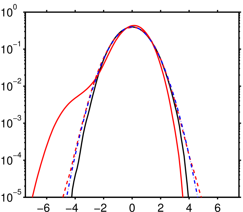
$u^{\prime}/\sigma(u^{\prime})$

pdf

pdf

$(b)$

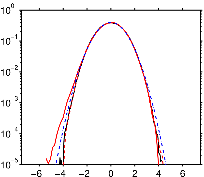
$u_{p}^{\prime}/\sigma(u_{p}^{\prime})$

Figure 14: Normalized probability density functions accumulated in the statistically stationary interval: $(a)$ fluid velocity; $(b)$ particle velocity. Line styles correspond to:  , case A-G0;  , vertical velocity in case AL-G120;      , horizontal velocity in case AL-G120;  $\,\cdot\,$ , Gaussian.

Figure 14 shows the normalized probability density functions (p.d.f.) of fluid and particle velocities, accumulated over the statistically stationary interval. It can be seen that the distributions of the velocities of both phases in the zero-gravity case A-G0 are approximately Gaussian. For both phases in case A-G0 we obtain a slightly smaller kurtosis value than for a Gaussian distribution, i.e. $K=2.83$ for the fluid and $K=2.82$ for the particle velocity. This result is fully consistent with case S2 of Yeo et. al.⁸ who report a value of 2.81 for the particle velocity kurtosis.

Concerning the finite-gravity case AL-G120, we observe that the horizontal velocity components of both phases remain essentially Gaussian distributed. The vertical fluid velocity component, on the other hand, exhibits a significant negative skewness which amounts to $S=-0.78$. This shape of the p.d.f. can be explained by the occurrence of wakes downstream of the settling particles which constitute predominantly negative fluctuations in the vertical fluid velocity field. A similar effect has been previously reported in Ref.3 for heavy particles settling in vertically-oriented turbulent channel flow. The vertical particle velocity component in case AL-G120 is also negatively skewed, albeit to a lesser degree ($S=-0.10$). This latter result implies that the particle motion is partially affected by the skewed fluid velocity field, again consistent with observations in channel flow³.

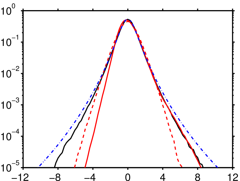
$a_{p}^{\prime}/\sigma(a_{p}^{\prime})$

pdf

Figure 15: Normalized probability density functions of particle acceleration. Line styles correspond to:  , case A-G0;  , vertical component in case AL-G120;      , horizontal component in case AL-G120;  $\,\cdot\,$ , log-normal fit of Qureshi et al.⁴⁷.

Let us now turn to the linear particle acceleration $\mathbf{a}_{p}=(a_{p,1},a_{p,2},a_{p,3})$, which is obtained from the following equation:

$$\rho_{p}V_{p}\mathbf{a}_{p}=\mathbf{F}^{(H)}+\mathbf{F}^{(B)}+\mathbf{F}^{(C)}\,,$$ (21)

where $\mathbf{F}^{(H)}$ is the hydrodynamic force, $\mathbf{F}^{(B)}$ the submerged weight and $\mathbf{F}^{(C)}$ the force contribution from particle-particle contact (cf. appendix F for details of the present numerical implementation). The statistics of particle acceleration presented in the present section have been computed after removing all samples corresponding to colliding spheres⁴. Let us note at this point that the mean collision-free interval for a particle amounts to $4.2T_{e}$ ($2.7T_{e}$) in case A-G0 (AL-G120).

The particle acceleration variance normalized in Kolmogorov scales $A_{\alpha}\equiv\langle a_{p,\alpha}^{\prime}a_{p,\alpha}^{\prime}\rangle_{t}\eta^{2/3}/\varepsilon^{4/3}$ (no summation over the index for the spatial direction $\alpha$) measures $A_{\alpha}=1.07$ in case A-G0. This value is close to the one in case S2 of Yeo et al.⁸ who obtain $A_{\alpha}=0.88$. The difference might be related to the effect of inter-particle contact in those author’s simulations performed at a substantially higher solid volume fraction. Note that the acceleration variance data of Homann & Bec⁷ are not directly comparable to our present data, since their simulation was run at much lower Reynolds number, and it is well known at least for fluid particles⁴⁸ that the value of $A_{\alpha}$ exhibits a significant Reynolds-number dependence.

The p.d.f. of particle acceleration is shown in figure 15 along with a log-normal distribution as first proposed by Mordant et al.⁴⁹ and fitted to experimental data by Qureshi et al.⁵⁰ with a value of the kurtosis of $K=8.37$; this fit was later shown⁴⁷ to provide a reasonable match of experimentally determined particle acceleration p.d.f.s over a range of relative particle sizes and density ratios. In the figure it can be seen that the acceleration data of our case A-G0 are consistent with the experimental fit. Similar to Yeo et al.⁸, however, we obtain a smaller value of the kurtosis of $K=6.46$ (their reported value is $K=6.24$). The data of Homann & Bec⁷ for neutrally-buoyant single particles suggest a decrease of the kurtosis from values of $K\approx 8$ to $K\approx 6$ taking place at $D/\eta\approx 7$; however, due to the smaller number of samples in that study their data do not allow for a more precise comparison.

When gravity is non-zero, the particle acceleration statistics become non-isotropic. The vertical (horizontal) component in case AL-G120 exhibits a kurtosis of $K=5.44$ ($K=3.94$), i.e. values which are both smaller than in the zero-gravity case. In addition the vertical component is positively skewed with $S=0.63$. While the reduction of the kurtosis in the presence of gravity deserves further analysis, the skewness of the vertical component of particle acceleration can be linked to the non-linear drag effect already discussed in section IV.2. A similar observation has been made in the context of particulate channel flow⁴.

$(a)$

$\tau/\tau_{\eta}$

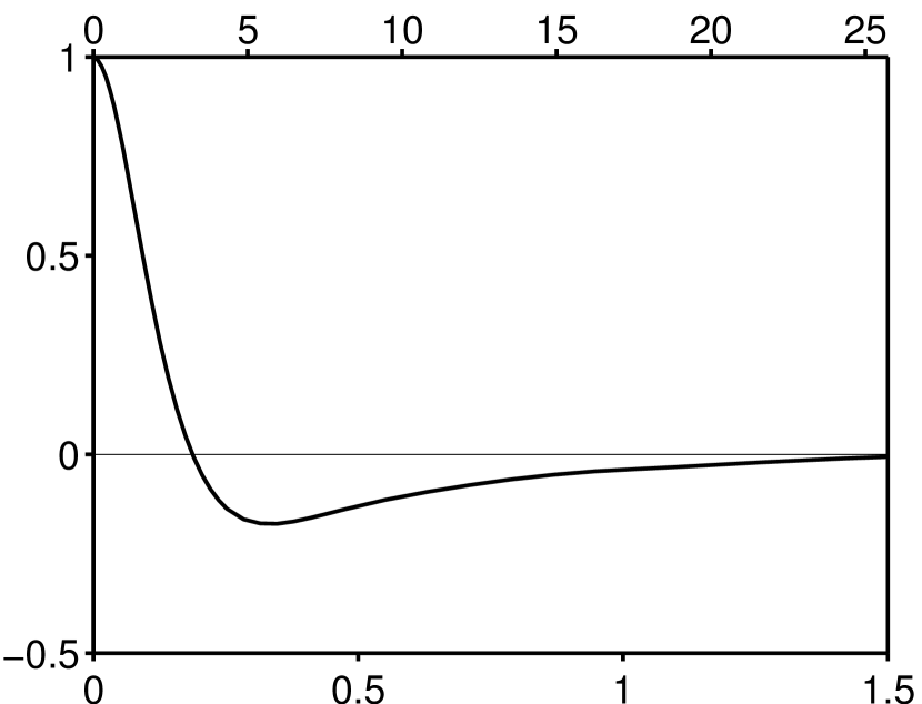
$\tau/T_{e}$

$\rho_{a}(\tau)$

$\rho_{a}(\tau)$

$(b)$

$\tau/\tau_{\tilde{\eta}}$

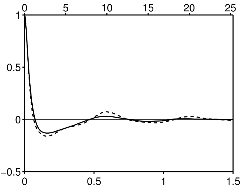
$\tau/T_{\tilde{e}}$

Figure 16: Auto-correlation function of particle acceleration: $(a)$ case A-G0; $(b)$ case AL-G120. In $(b)$ the solid line corresponds to the vertical component, while the dashed line stands for the horizontal ones. Note also that in $(b)$ the modified dissipation $\tilde{\varepsilon}$ (defined in 18) has been used to compute modified time-scales $\tau_{\tilde{\eta}}$ and $T_{\tilde{e}}$.

Information on the time scales of forces acting on the particles is provided in figure 16 which shows the auto-correlation of acceleration, $\rho_{a}(\tau)$. The shape of the auto-correlation function in case A-G0 is fully consistent with the data of Ref.^{8, 7}, exhibiting first a rapid decay, a subsequent negative loop, and a final slow approach to zero from below. The first zero-crossing in the present case A-G0 occurs at $\tau_{zero}/\tau_{\eta}=3.11$, while Yeo et al.⁸ obtain $\tau_{zero}/\tau_{\eta}=3.2$ in their case S2, and Homann & Bec⁷ report a value of $\tau_{zero}/\tau_{\eta}=2.5$ for a single neutrally-buoyant particle with $D/\eta=6$.

In comparison the auto-correlation in case AL-G120 exhibits a much faster initial decay, with a zero-crossing at $\tau_{zero}/\tau_{\tilde{\eta}}=1.26$ ($1.13$) for the vertical (horizontal) component. This faster decorrelation can be attributed to the crossing-trajectory effect⁵¹ due to settling particles spending a smaller amount of time under the influence of a given flow structure as compared to a zero-gravity case. It can also be observed that the auto-correlation in case AL-G120 mildly oscillates around the zero value. Although the amplitude of the oscillation is very small ($0.03$ and $0.07$ in the vertical and horizontal component, respectively), it is instructive to investigate it further. The oscillation period measures $0.59T_{e}$, which corresponds roughly to one half of the value of the particle return time based upon the time-averaged settling velocity and the vertical extent of the periodic computational domain, viz. $T_{r}={\cal L}_{z}/\langle w_{rel}\rangle_{t}=1.23T_{e}$. Therefore, this slightly oscillatory behavior of $\rho_{a}(\tau)$ is an artifact of the finite vertical domain size. Since the secondary maximum of $\rho_{a}$ is located at a temporal separation equal to one half of the return time, and because this time interval is not larger than the large-eddy time-scale, the oscillations of $\rho_{a}$ are most likely caused by particles having a certain probability to interact repeatedly with the same flow structure while settling through the vertically periodic domain. Consequently, this feature can be linked to the two-point correlation function of figure 7$(b)$ which was found to remain finite at the largest separations in the vertical direction. It can therefore be concluded that the presently chosen vertical elongation of the computational domain does not completely prevent the Lagrangian signals to be affected by the finite return time. It does, however, alleviate the restrictions stemming from the long vertical extent of the wakes left behind by settling particles.

V Summary and conclusion

In the present study we have considered the motion of finite-size, inertial, spherical particles in statistically stationary homogeneous turbulence without mean velocity gradients. The Navier-Stokes equations for a constant density fluid are solved with the aid of an immersed boundary technique for imposing the no-slip condition at the fluid-particle interfaces while using a fixed computational grid. The turbulent motion is generated by the large-scale random forcing procedure of Eswaran and Pope¹⁸. Since only a limited number of Fourier modes are forced, full transforms of the forcing fields can be avoided through a direct evaluation of the Fourier series in physical space. This means that the computation of the forcing term can be done efficiently in local memory, avoiding any inter-processor communication.

Since our objective is to understand the influence of gravity upon the fluid-particle interaction, special care has been taken to address the requirements due to particles which are upon average settling with respect to the mean fluid-phase velocity. Therefore, we have considered the case of isotropically-forced turbulence in vertically elongated computational domains.

We have carried out simulations in medium-sized systems at low to moderate turbulent Reynolds numbers. An initial validation is performed for single-phase flow. The comparison with reference data¹² in cubical boxes shows an excellent agreement at the corresponding Reynolds number. Concerning elongated boxes we obtain essentially the same flow statistics (including a very good isotropy) when the domain is elongated by a factor of two in one spatial direction while only every second Fourier wavenumber in that direction is forced. Since the spectral energy content of the largest modes which are not forced (i.e. those interspersed between the forced ones) does not remain zero under the dynamics of the Navier-Stokes equations, the simulated field in an elongated box is not a simple copy of a corresponding field from a cubical simulation. At the same time two-point correlation data show that the fields in the cubical sub-volumes of the elongated simulation remain somewhat correlated. However, we also show that once settling particles are added to the simulation in a vertically-elongated box, the vertical two-point correlation of the velocity field is reduced by the fact that the particle positions only possess the fundamental periodicity.

Particulate flow simulations involving a dilute suspension of inertial particles at Galileo numbers $Ga=0$ and $120$ have been performed at low turbulent Reynolds number. The first conclusion is that the random forcing procedure does not pose any numerical stability problems, allowing us to obtain a well-defined statistically stationary state and to collect statistics over arbitrarily long temporal intervals. The zero-gravity case has been thoroughly validated with respect to available experimental and numerical data.

Concerning the particulate flow case with finite gravity, the present simulations suggest that the average particle settling velocity is reduced by 1.5% with respect to the one of an isolated particle in quiescent surroundings. An evaluation of the standard non-linear drag model⁴⁴ with the present parameters yields the correct trend, and non-linear drag is also a likely candidate for the observed positive skewness of the p.d.f. of vertical particle acceleration. On the other hand, the p.d.f.s of the vertical component of the fluid and of the particle velocity in this case become negatively skewed, presumably as a result of the presence of mean wakes, and similarly to previous results in vertical plane channel flow³. Finally, the crossing-trajectories effect leads to a substantial reduction of the auto-correlation of the particle acceleration in the finite-gravity case as compared to zero gravity.

The present study shows that the simulation of forced turbulent flow seeded with fully-resolved, settling particles, satisfying the requirements mentioned in the introduction, is feasible today. Our first results at relatively low Reynolds number obtained in medium-sized systems already bear some interesting features. In the future we will consider larger systems while increasing the Reynolds number. This will allow us to investigate in more detail the interaction between the finite-size particles and the turbulent flow structures.

Appendix A Evaluating the turbulence forcing in physical space

The formula for evaluating the turbulence forcing term at a discrete physical space grid node $\mathbf{x}_{ijk}=(x_{i},y_{j},z_{k})$ from given discrete Fourier coefficients $\hat{\mathbf{f}}^{(t)}(\bm{\kappa}_{lmn})=\hat{\mathbf{f}}^{(t)}(\kappa_{1,l},\kappa_{2,m},\kappa_{3,n})$ can be written as follows:

$$\mathbf{f}^{(t)}(\mathbf{x}_{ijk})=\sum_{l=-N_{f}}^{N_{f}}\sum_{m=-N_{f}}^{N_{f}}\sum_{n=-N_{f}}^{N_{f}}\left(\hat{\mathbf{f}}_{lmn}^{(t)}\exp(I\kappa_{1,l}x_{i})\exp(I\kappa_{2,m}y_{j})\exp(I\kappa_{3,n}z_{k})\right)\,,\quad\forall\,\,i,j,k\,,$$ (22)

where for each direction $N_{f}$ is the number of positive Fourier wavenumbers which receive a non-zero forcing contribution. The $i$th element of the wavenumber vector in the $\alpha$-direction is defined as:

$$\kappa_{\alpha,i}=\frac{2\pi i}{{\cal L}_{\alpha}}\,.$$ (23)

Note that the coefficients for the negative wavenumbers in one of the coordinate directions are actually reconstructed from the corresponding positive ones taking into account that the result in physical space is real-valued. A direct implementation of (22) corresponds to a sextuple loop with ${\cal O}(N_{f}^{3}N_{x,loc}N_{y,loc}N_{z,loc})$ operations, where $N_{x,loc}$, $N_{y,loc}$, $N_{z,loc}$ are the numbers of physical space grid points in each coordinate direction which are held in local memory by a given process in a three-dimensional Cartesian domain decomposition.

In practice the summation in (22) is split up into three consecutive steps, as shown in the following:

$$\mathbf{A}_{mni} = \sum_{l=-N_{f}}^{N_{f}}\left(\hat{\mathbf{f}}_{lmn}^{(t)}\exp(I\kappa_{1,l}x_{i})\right)\,,\quad\forall\,\,m,n,i\,,$$ (24a)

$$\mathbf{B}_{nij} = \sum_{m=-N_{f}}^{N_{f}}\left(\mathbf{A}_{mni}\exp(I\kappa_{2,m}y_{j})\right)\,,\quad\forall\,\,n,i,j\,,$$ (24b)

$$\mathbf{f}^{(t)}(\mathbf{x}_{ijk}) = \sum_{n=-N_{f}}^{N_{f}}\left(\mathbf{B}_{nij}\exp(I\kappa_{3,n}z_{k})\right)\,,\quad\forall\,\,i,j,k\,.$$ (24c)

The operation count for each of the steps in (24) is ${\cal O}(N_{f}^{3}N_{x,loc})$, ${\cal O}(N_{f}^{2}N_{x,loc}N_{y,loc})$, and ${\cal O}(N_{f}N_{x,loc}N_{y,loc}N_{z,loc})$, respectively.

Appendix B The time-splitting algorithm for particulate flow with turbulence forcing

In the present numerical method the flow equations are discretized in time with the aid of a three-step Runge-Kutta scheme for the advection terms in conjunction with a Crank-Nicolson scheme for the viscous terms. In each Runge-Kutta sub-step (with super-script index “$k$”) a fractional step procedure is employed, consisting of: (i) a first predictor step which serves to compute a preliminary flow field $\tilde{\mathbf{u}}$ from which the necessary force density $\mathbf{f}^{(ibm)}$ for imposing a no-slip condition at the fluid-solid interface of each particle is deduced; (ii) a second predictor step yielding a solution $\mathbf{u}^{\ast}$ to the momentum equation which does in general not verify the divergence-free condition; (iii) a corrector step which yields a divergence-free velocity field $\mathbf{u}^{k}$ through a pressure-projection operation. Therefore, the time-discretized Navier-Stokes equations for the $k$th Runge-Kutta step can be expressed as the following sequence of operations:

$$\tilde{\mathbf{u}} = \mathbf{u}^{k-1}+\Delta t\left(2\alpha_{k}\nu\nabla^{2}\mathbf{u}^{k-1}-2\alpha_{k}\nabla p^{k-1}\right.$$ (25a)

$$\left.-\gamma_{k}\left((\mathbf{u}\cdot\nabla)\mathbf{u}\right)^{k-1}-\zeta_{k}\left((\mathbf{u}\cdot\nabla)\mathbf{u}\right)^{k-2}+2\alpha_{k}\mathbf{f}^{(t)}(t^{n})\right)\,,$$

$$\tilde{{U}}_{\beta}(\mathbf{X}_{l}^{(m)}) = \sum_{ijk}\tilde{{u}}_{\beta}(\mathbf{x}_{ijk}^{(\beta)})\,\delta_{h}(\mathbf{x}_{ijk}^{(\beta)}-\mathbf{X}_{l}^{(m)})\,\Delta x^{3}\,,\quad\forall\,l;\,m;\,\beta$$ (25b)

$$\mathbf{F}(\mathbf{X}_{l}^{(m)}) = \frac{\mathbf{U}^{(d)}(\mathbf{X}_{l}^{(m)})-\tilde{\mathbf{U}}(\mathbf{X}_{l}^{(m)})}{\Delta t}\,,\quad\qquad\qquad\forall\,l;\,m$$ (25c)

$${f}_{\beta}^{(ibm)}(\mathbf{x}_{ijk}) = \sum_{m=1}^{N_{p}}\sum_{l=1}^{N_{L}}{F}_{\beta}(\mathbf{X}_{l}^{(m)})\,\delta_{h}(\mathbf{x}_{ijk}^{(\beta)}-\mathbf{X}_{l}^{(m)})\,\Delta V_{l}^{(m)}\,,\quad\forall\,\beta;\,i;\,j;\,k$$ (25d)

$$\nabla^{2}\mathbf{u}^{\ast}-\frac{\mathbf{u}^{\ast}}{\alpha_{k}\nu\Delta t} = -\frac{1}{\nu\alpha_{k}}\left(\frac{\tilde{\mathbf{u}}}{\Delta t}+\mathbf{f}^{(ibm)}-\langle\mathbf{f}^{(ibm)}\rangle_{\Omega}\right)+\nabla^{2}\mathbf{u}^{k-1}\,,$$ (25e)

$$\nabla^{2}\phi = \frac{\nabla\cdot\mathbf{u}^{\ast}}{2\alpha_{k}\Delta t}\,,$$ (25f)

$$\mathbf{u}^{k} = \mathbf{u}^{\ast}-2\alpha_{k}\Delta t\nabla\phi\,,$$ (25g)

$$p^{k} = p^{k-1}+\phi-\alpha_{k}\Delta t\,\nu\nabla^{2}\phi\,,$$ (25h)

where the set of coefficients $\alpha_{k}$, $\gamma_{k}$, $\zeta_{k}$ (with $k=1,2,3$) is given in Ref.52. The intermediate variable $\phi$ is the so-called “pseudo-pressure”, which together with the predictor velocity fields $\tilde{\mathbf{u}}$ and $\mathbf{u}^{\ast}$ is discarded at the end of the Runge-Kutta sub-step. The upper-case letters denote quantities evaluated at a set of Lagrangian force points located at positions $\mathbf{X}_{l}^{(m)}$ on the surface of the $m$th particle (out of a total number of $N_{p}$ particles), the sub-script ranging as $l=1\ldots N_{L}$. The transfer between Eulerian coordinates (i.e. staggered grid nodes $\mathbf{x}_{ijk}^{(\beta)}$ associated with the $\beta$-component of velocity) and Lagrangian force points is performed with the aid of Peskin’s regularized delta function $\delta_{h}$, with a forcing volume $\Delta V_{l}^{(m)}$ associated to each Lagrangian force point. The quantity $\mathbf{U}^{(d)}(\mathbf{X}_{l}^{(m)})$ in (25c) represents the current local velocity of the $m$th solid particle’s force point with index $l$. It is directly linked to the current values of the particle’s translational and angular velocity, which in turn, are obtained from integrating the Newton equations for rigid body motion. Also note that the turbulence forcing field $\mathbf{f}^{(t)}$ is not updated during the Runge-Kutta sub-steps; instead it is evaluated once per full time step.

In the case of triply-periodic boundary conditions, the spatial average of the force term needs to be subtracted from the momentum equation in order to allow the system to attain a statistically stationary state ^{29, 30}. More specifically, at each time step we compute the following average

$$\langle\mathbf{f}^{(ibm)}\rangle_{\Omega}(t)=\frac{1}{||\Omega||}\int_{\Omega}\mathbf{f}^{(ibm)}(\mathbf{x},t)\mbox{d}\mathbf{x}\,,$$ (26)

which is then subtracted from the momentum balance (cf. Helmholtz equation 25e during the predictor step).

Appendix C Definition of averaging operators

Here we use the same averaging procedures as in Ref.11 which will be briefly summarized in the following. We define a fluid-phase indicator function $\Phi_{f}(\mathbf{x},t)$, which specifies whether a given point $\mathbf{x}$ at time $t$ is located inside the region $\Omega_{f}(t)$ occupied by the fluid at time $t$, viz.

$$\Phi_{f}(\mathbf{x},t)=\left\{\begin{array}[]{l l}1\qquad\mbox{if}\quad\mathbf{x}\in\Omega_{f}(t)\\ 0\qquad\mbox{else}\\ \end{array}\right.\,,$$ (27)

and the corresponding indicator function for the particle phase $\Phi_{p}(\mathbf{x},t)$ is then simply given by $\Phi_{p}=1-\Phi_{f}$. The fluid-phase averaging for any fluid-related quantity $\psi_{f}(\mathbf{x})$ is denoted by the operator $\langle\cdot\rangle_{\Omega_{f}}$, while the indiscriminate average (over the entire computational domain) is denoted by $\langle\cdot\rangle_{\Omega}$. These two averages are related by the following identity:

$$\langle\psi_{f}\rangle_{\Omega_{f}}=\frac{||\Omega||}{||\Omega_{f}||}\langle\psi_{f}\,\Phi_{f}\rangle_{\Omega}\,.$$ (28)

The operator $\langle\cdot\rangle_{p}$ for a given quantity $\psi_{p}^{(i)}$ related to the $i$th particle represents the instantaneous average over the number of particles. Finally, the time average is indicated by the operator $\langle\cdot\rangle_{t}$.

Appendix D A priori estimation of turbulence forcing parameters

Eswaran and Pope¹⁸ provide estimates of the dissipation rate, the Kolmogorov length scale and the Reynolds number based upon the values chosen for the free parameters of their forcing scheme (i.e. $T_{L}$, $\kappa_{f}$, $\epsilon^{\ast}$). They first introduce a non-dimensional forcing time scale $T_{L}^{*}=T_{L}(\varepsilon^{*})^{1/3}\kappa_{0}^{2/3}$ (where $\kappa_{0}$ is the lowest wavenumber in Fourier space). It is then proposed that the quantity $\varepsilon_{T}^{*}=4\varepsilon^{*}N_{f}/(1+T_{L}^{*}N_{f}^{1/3}/\beta)$ should serve as an estimate for the dissipation rate ($N_{f}$ being the total number of forced wavenumbers, and $\beta=0.8$ an adjusted constant). From this an estimate for the Kolmogorov length can be obtained from $\eta_{T}=(\nu^{3}/\varepsilon_{T}^{*})^{1/4}$. Furthermore, Eswaran and Pope¹⁸ suggest the following empirical expression for estimating the Taylor-scale Reynolds number: $Re_{\lambda}^{T}=8.5/((\eta_{T}\kappa_{0})^{5/6}N_{f}^{2/9})$.

In our simulations we have indeed confirmed that the Kolmogorov length $\eta$ is reasonably well predicted by the quantity $\eta_{T}$. However, the Reynolds number $Re_{\lambda}$ is overpredicted by the quantity $Re_{\lambda}^{T}$ (by approximately 14% in case A and by 28% in case B). This discrepancy might be due to the fact that we are considering here Reynolds numbers larger than the ones used in the original work.

In what follows an alternative estimate is proposed. We define a macroscopic scale $\mathcal{L}_{c}=2\pi/\kappa_{c}$ from the central wavenumber of the forced interval $\kappa_{c}=(\kappa_{0}+\kappa_{f})/2$, which should take values close to the large-eddy length-scale $L$. We can then derive a large-scale Reynolds number $Re_{c}=\mathcal{L}_{c}u_{rms}/\nu\approx Re_{L}$. Therein $u_{rms}$ is estimated by assuming that $\varepsilon\approx\varepsilon_{T}^{*}$ and that $T_{e}=u^{2}_{rms}/\varepsilon\approx T_{L}$. Using the relation between large-scale Reynolds number and Taylor-scale Reynolds number⁴², $Re_{\lambda}=(20Re_{L}/3)^{1/2}$, we arrive at the following estimate based upon the forcing parameters: $Re_{\lambda}^{T2}=(20{\cal L}_{c}(T_{L}\varepsilon_{T}^{*})^{1/2}/(3\nu))^{1/2}$. It is found that the resulting values of $Re_{\lambda}^{T2}$ provide a better match to our simulation data, with 8% (3%) discrepancy with respect to $Re_{\lambda}$ in case A (case B).

In the main text we use as a priori reference scales for normalizing the dissipation rate and the kinetic energy the quantities $\varepsilon_{ref}=\varepsilon_{T}^{*}$ and $k_{ref}=3\varepsilon_{T}^{*}T_{L}/2$, respectively, which are purely based upon the imposed forcing parameters.

Appendix E Fluid velocity probabilities in the single-phase case

$(a)$

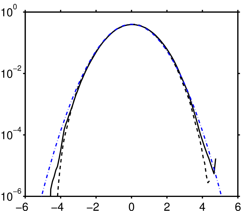
$u^{\prime}/u_{rms}$

pdf

pdf

$(b)$

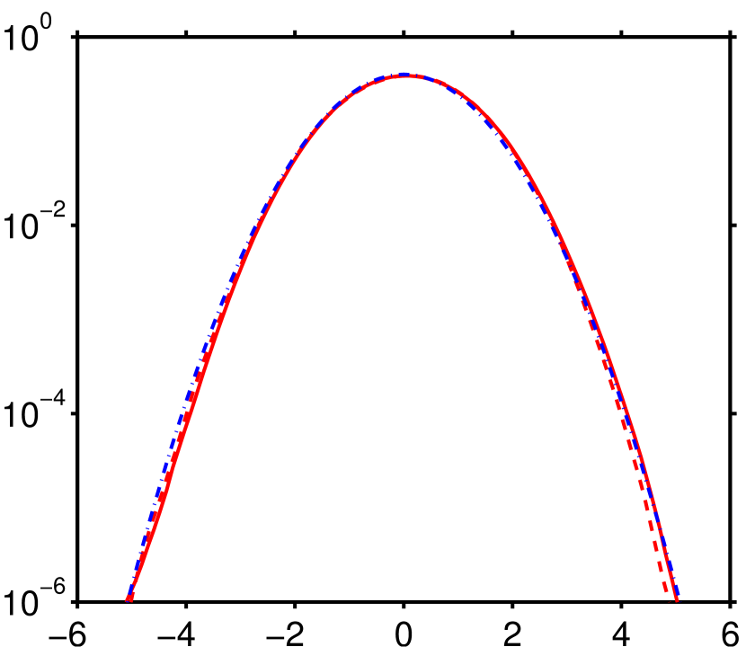
$u^{\prime}/u_{rms}$

Figure 17: Probability density functions of fluid velocity fluctuations in the single-phase case. Data at lower Reynolds number is shown in $(a)$:  , case A,      , case AL. The graph in $(b)$ collects the data at higher Reynolds number:  , case B,      , case BL. The blue chain-dotted line shows a Gaussian reference curve.

For the sake of completeness, the p.d.f. of the fluid velocity flucutations in the single-phase cases of section III are shown in figure 17. It can be seen that while at lower Reynolds number there exists a slight deviation from Gaussianity, the higher Reynolds data almost perfectly collapse with the Gaussian reference curve.

Appendix F Reformulation of the kinetic energy budget

The purpose of the present appendix is to bring the two-way coupling term (10) in the box-averaged kinetic energy equation (7) into a more tractable form.

Since the force which imposes the no-slip condition at the fluid-particle interfaces, $\mathbf{f}^{(ibm)}$, is localized around the particles, any volume integral involving $\mathbf{f}^{(ibm)}$ can be expressed as a sum of integrals over each particle’s surface, e.g. we can write:

$$\langle\mathbf{u}\cdot\mathbf{f}^{(ibm)}\rangle_{\Omega}\equiv\frac{1}{||\Omega||}\int_{\Omega}\left(\mathbf{u}\cdot\mathbf{f}^{(ibm)}\right)\mbox{d}\mathbf{x}=\frac{1}{||\Omega||}\sum_{i=1}^{N_{p}}\int_{\mathbf{x}\in{\cal S}^{(i)}}\left(\mathbf{u}\cdot\mathbf{f}^{(ibm)}\right)\mbox{d}\mathbf{x}\,,$$ (29)

where $||\Omega||$ is the volume of the triply-periodic computational domain and ${\cal S}^{(i)}$ is the surface of the $i$th particle. Substituting the no-slip value at the surface of the particle, i.e.

$$\mathbf{u}(\mathbf{x}\in{\cal S}^{(i)}(t),t)=\mathbf{u}_{p}^{(i)}(t)+\bm{\omega}_{p}^{(i)}(t)\times\mathbf{r}^{(i)}(\mathbf{x},t)\,,$$ (30)

into (29) yields

$$\langle\mathbf{u}\cdot\mathbf{f}^{(ibm)}\rangle_{\Omega} = \frac{1}{||\Omega||}\sum_{i=1}^{N_{p}}\left[\mathbf{u}_{p}^{(i)}\cdot\int_{\mathbf{x}\in{\cal S}^{(i)}}\mathbf{f}^{(ibm)}\mbox{d}\mathbf{x}+\bm{\omega}_{p}^{(i)}\cdot\int_{\mathbf{x}\in{\cal S}^{(i)}}\left(\mathbf{r}^{(i)}\times\mathbf{f}^{(ibm)}\right)\mbox{d}\mathbf{x}\right],$$ (31)

where the vector $\mathbf{r}$ pointing from the $i$th particle’s center to a location $\mathbf{x}$ on its surface has been defined as $\mathbf{r}^{(i)}(\mathbf{x},t)=\mathbf{x}-\mathbf{x}_{p}^{(i)}(t)$, and the invariance with respect to circular shifts of the operands of the triple scalar product $(\bm{\omega}_{p}\times\mathbf{r})\cdot\mathbf{f}^{(ibm)}$ has been used.

In order to replace the first integral on the r.h.s. of (31) we resort to the Newton-Euler equation for rigid body motion of a spherical particle which reads in our present numerical framework³:

$$V_{p}\left(\rho_{p}-\rho_{f}\right)\frac{\mbox{d}\mathbf{u}_{p}^{(i)}}{\mbox{d}t}=-\rho_{f}\int_{\mathbf{x}\in{\cal S}^{(i)}}\mathbf{f}^{(ibm)}\,\mbox{d}\mathbf{x}+V_{p}\left(\rho_{p}-\rho_{f}\right)\mathbf{g}+\mathbf{F}_{c}^{(i)}\,,$$ (32)

where $\mathbf{F}_{c}^{(i)}$ is the sum of the forces due to solid contact of the $i$th particle with any other particle. Note that $\mathbf{F}_{c}^{(i)}$ is a force (unit: mass times acceleration), while $\mathbf{f}^{(ibm)}$ is a force density (force per unit mass). The Newton-Euler equation for the angular acceleration in the context of our immersed boundary approach reads ²²:

$$I_{p}\frac{\mbox{d}\bm{\omega}_{p}^{(i)}}{\mbox{d}t}\left(1-\frac{\rho_{f}}{\rho_{p}}\right)=-\rho_{f}\int_{\mathbf{x}\in{\cal S}^{(i)}}\left(\mathbf{r}^{(i)}\times\mathbf{f}^{(ibm)}\right)\mbox{d}\mathbf{x}\,,$$ (33)

where the moment of inertia for a sphere is $I_{p}=2\rho_{p}V_{p}R^{2}/5$ (with $R=D/2$ the sphere radius). Note that in writing (33) we have assumed that the collision model does not generate torque on the particles (as is indeed the case here) and, therefore, no collision-related term enters this equation; the opposite is true if the collision model has a tangential component.

With the aid of relations (32) and (33) the integrals appearing in (31) can be eliminated. Similarly, relation (32) can be used to eliminate the integral $\langle\mathbf{f}^{(ibm)}\rangle_{\Omega}$ appearing in the second term on the right-hand side of relation (10). Finally, we obtain the following expression for the fluid-particle coupling term:

$$\Psi^{(p)}(t)=\phi_{s}\left(\frac{\rho_{p}}{\rho_{f}}-1\right)\mathbf{u}_{rel,\Omega}\cdot\mathbf{g}+\Psi^{(p)}_{accel}(t)+\Psi^{(p)}_{coll}(t)\,,$$ (34)

where we have defined an apparent slip velocity with respect to the box-averaged velocity field:

$$\mathbf{u}_{rel,\Omega}=\langle\mathbf{u}_{p}^{(i)}\rangle_{p}-\langle\mathbf{u}\rangle_{\Omega}\,.$$ (35)

The two expressions regrouping all acceleration terms and the inter-particle collision term, respectively, read as follows:

$$\Psi^{(p)}_{accel}(t) = \phi_{s}\left(\frac{\rho_{p}}{\rho_{f}}-1\right)\left[\langle\mathbf{u}\rangle_{\Omega}\cdot\left\langle\frac{\mbox{d}\mathbf{u}_{p}}{\mbox{d}t}\right\rangle_{p}-\left\langle\mathbf{u}_{p}\cdot\frac{\mbox{d}\mathbf{u}_{p}}{\mbox{d}t}\right\rangle_{p}-\frac{D^{2}}{10}\left\langle\bm{\omega}_{p}\cdot\frac{\mbox{d}\bm{\omega}_{p}}{\mbox{d}t}\right\rangle_{p}\right],$$ (36a)

$$\Psi^{(p)}_{coll}(t) = \frac{1}{||\Omega||}\sum_{i=1}^{N_{p}}\mathbf{u}_{p}^{(i)}\cdot\frac{\mathbf{F}_{c}^{(i)}}{\rho_{f}}\,.$$ (36b)

Appendix G Voronoï tesselation analysis

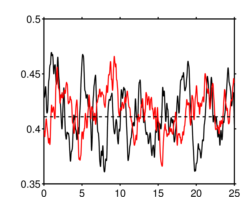
$t/T_{e}$

$\sigma(V^{(i)}/\langle V^{(i)}\rangle_{p,t})$

Figure 18: Time evolution of the standard deviation of the normalized volume of the cells of the three-dimensional Voronoï tesselation with the particle centers as “sites”. Line styles correspond to:  , case A-G0 (time-evaraged value $0.418$);  , case AL-G120 (time-evaraged value $0.416$),      , value of $0.411$, corresponding to particles with the same solid volume fraction, distributed non-overlappingly by means of a random Poisson process ¹¹.

An analysis of the spatial particle distribution by means of Voronoï tesselation⁵³ has been performed in the same manner as in Ref.11. The Voronoï cells’ volume is an indicator for the inverse of a concentration; the p.d.f. of the normalized cell volumes being typically gamma-distributed⁵⁴, with the standard-deviation being a good scalar indicator of clustering. According to the data shown in figure 18 in both cases A-G0 and AL-G120 the standard deviations of the Voronoï cell volumes fluctuate in time around the value which corresponds to a particle distribution through a random Poisson process. Therefore, we conclude that significant particle clustering does not occur.

References

- Pan and Banerjee 1997 Y. Pan and S. Banerjee, “Numerical investigation of the effects of large particles on wall-turbulence,” Phys. Fluids 9, 3786–3807 (1997).
- Kajishima and Takiguchi 2002 T. Kajishima and S. Takiguchi, “Interaction between particle clusters and particle-induced turbulence,” Int. J. Heat Fluid Flow 23, 639–646 (2002).
- Uhlmann 2008 M. Uhlmann, “Interface-resolved direct numerical simulation of vertical particulate channel flow in the turbulent regime,” Phys. Fluids 20, 053305 (2008).
- García-Villalba, Kidanemariam, and Uhlmann 2012 M. García-Villalba, A. Kidanemariam, and M. Uhlmann, “DNS of vertical plane channel flow with finite-size particles: Voronoi analysis, acceleration statistics and particle-conditioned averaging,” Int. J. Multiphase Flow 46, 54–74 (2012).
- Picano, Breugem, and Brandt 2015 F. Picano, W.-P. Breugem, and L. Brandt, “Turbulent channel flow of dense suspensions of neutrally buoyant spheres,” J. Fluid Mech. 764, 463–487 (2015).
- Ten Cate et al. 2004 A. Ten Cate, J. Derksen, L. Portella, and H. Van Den Akker, “Fully resolved simulations of colliding monodisperse spheres in forced isotropic turbulence,” J. Fluid Mech. 519, 233–271 (2004).
- Homann and Bec 2010 H. Homann and J. Bec, “Finite-size effects in the dynamics of neutrally buoyant particles in turbulent flow,” J. Fluid Mech. 651, 81–91 (2010).
- Yeo et al. 2010 K. Yeo, S. Dong, E. Climent, and M. Maxey, “Modulation of homogeneous turbulence seeded with finite size bubbles or particles,” Int. J. Multiphase Flow 36, 221–233 (2010).
- Doychev and Uhlmann 2010 T. Doychev and M. Uhlmann, “A numerical study of finite size particles in homogeneous turbulent flow,” in Proceedings of the 7th International Conference on Multiphase Flow, edited by S. Balachandar and J. S. Curtis (University of Florida, Gainesville (USA), 2010).
- Lucci, Ferrante, and Elghobashi 2010 F. Lucci, A. Ferrante, and S. Elghobashi, “Modulation of isotropic turbulence by particles of Taylor length-scale size,” J. Fluid Mech. 650, 5–55 (2010).
- Uhlmann and Doychev 2014 M. Uhlmann and T. Doychev, “Sedimentation of a dilute suspension of rigid spheres at intermediate Galileo numbers: the effect of clustering upon the particle motion,” J. Fluid Mech. 752, 310–348 (2014), 1406.1667 .
- Jiménez et al. 1993 J. Jiménez, A. Wray, P. Saffman, and R. Rogallo, “The structure of intense vorticity in isotropic turbulence,” J. Fluid Mech. 255, 65–90 (1993).
- Sullivan and Mahalingam 1994 N. Sullivan and S. Mahalingam, “Deterministic forcing of homogeneous, isotropic turbulence,” Phys. Fluids 6, 1612–1614 (1994).
- Ishihara et al. 2007 T. Ishihara, Y. Kaneda, M. Yokokawa, K. Itakura, and A. Uno., “Small-scale statistics in high-resolution direct numerical simulation of turbulence: Reynolds number dependence of one-point velocity gradient statistics,” J. Fluid Mech. 592, 335–366 (2007).
- Yeung, Donzis, and Sreenivasan 2012 P. Yeung, D. Donzis, and K. Sreenivasan, “Dissipation, enstrophy and pressure statistics in turbulence simulations at high Reynolds numbers,” J. Fluid Mech. 700, 5–15 (2012).
- Lundgren 2003 T. Lundgren, “Linearly forced isotropic turbulence,” in Annual Research Briefs ((Center for Turbulence Research, Stanford), 2003) pp. 461–473.
- Rosales and Meneveau 2005 C. Rosales and C. Meneveau, “Linear forcing in numerical simulations of isotropic turbulence: Physical space implementations and convergence properties,” Phys. Fluids 17, 095106 (2005).
- Eswaran and Pope 1988 V. Eswaran and S. Pope, “An examination of forcing in direct numerical simulations of turbulence,” Comput. Fluids 16, 257–278 (1988).
- Alvelius 1999 K. Alvelius, “Random forcing of three-dimensional homogeneous turbulence,” Phys. Fluids 11, 1880 (1999).
- Naso and Prosperetti 2010 A. Naso and A. Prosperetti, “The interaction between a solid particle and a turbulent flow,” New J. Phys. 12 (2010).
- Lomholt and Maxey 2003 S. Lomholt and M. Maxey, “Force-coupling method for particulate two-phase flow: Stokes flow,” J. Comput. Phys. 184, 381 – 405 (2003).
- Uhlmann 2005 M. Uhlmann, “An immersed boundary method with direct forcing for the simulation of particulate flows,” J. Comput. Phys. 209, 448–476 (2005).
- Chan-Braun, García-Villalba, and Uhlmann 2011 C. Chan-Braun, M. García-Villalba, and M. Uhlmann, “Force and torque acting on particles in a transitionally rough open channel flow,” J. Fluid Mech. 684, 441–474 (2011).
- Kidanemariam et al. 2013 A. Kidanemariam, C. Chan-Braun, T. Doychev, and M. Uhlmann, “DNS of horizontal open channel flow with finite-size, heavy particles at low solid volume fraction,” New J. Phys. 15, 025031 (2013).
- Chan-Braun, García-Villalba, and Uhlmann 2013 C. Chan-Braun, M. García-Villalba, and M. Uhlmann, “Spatial and temporal scales of force and torque acting on wall-mounted spherical particles in open channel flow,” Phys. Fluids 25, 075103 (2013).
- Uhlmann and Dušek 2014 M. Uhlmann and J. Dušek, “The motion of a single heavy sphere in ambient fluid: a benchmark for interface-resolved particulate flow simulations with significant relative velocities,” Int. J. Multiphase Flow 59, 221–243 (2014).
- Kidanemariam and Uhlmann 2014a A. Kidanemariam and M. Uhlmann, “Interface-resolved direct numerical simulation of the erosion of a sediment bed sheared by laminar flow,” Int. J. Multiphase Flow 67, 174–188 (2014a).
- Kidanemariam and Uhlmann 2014b A. Kidanemariam and M. Uhlmann, “Direct numerical simulation of pattern formation in subaqueous sediment,” J. Fluid Mech. 750, R2 (2014b).
- Fogelson and Peskin 1988 A. Fogelson and C. Peskin, “A fast numerical method for solving the three-dimensional Stokes’ equations in the presence of suspended particles,” J. Comput. Phys. 79, 50–69 (1988).
- Höfler and Schwarzer 2000 K. Höfler and S. Schwarzer, “Navier-Stokes simulation with constraint forces: Finite-difference method for particle-laden flows and complex geometries,” Phys. Rev. E 61, 7146–7160 (2000).
- Glowinski et al. 1999 R. Glowinski, T.-W. Pan, T. Hesla, and D. Joseph, “A distributed Lagrange multiplier/fictitious domain method for particulate flows,” Int. J. Multiphase Flow 25, 755–794 (1999).
- Jimenez 1998 J. Jimenez, ed., A selection of test cases for the validation of large-eddy simulations of turbulent flows, AGARD Advisory Report No. 345 (NATO Advisory Group for Aerospace Research and Development, 1998).
- Amoura et al. 2010 Z. Amoura, V. Roig, F. Risso, and A.-M. Billet, “Attenuation of the wake of a sphere in an intense incident turbulence with large length scales,” Phys. Fluids 22, 055105 (2010).
- Bagchi and Balachandar 2004 P. Bagchi and S. Balachandar, “Response of the wake of an isolated particle to an isotropic turbulent flow,” J. Fluid Mech. 518, 95–123 (2004).
- Wu and Faeth 1994 J. Wu and G. Faeth, “Sphere wakes at moderate Reynolds numbers in a turbulent environment,” AIAA J. 32, 535–541 (1994).
- Legendre, Merle, and Magnaudet 2006 D. Legendre, A. Merle, and J. Magnaudet, “Wake of a spherical bubble or a solid sphere set fixed in a turbulent environment,” Phys. Fluids 18, 048102 (2006).
- Fede, Simonin, and Villedieu 2007 P. Fede, O. Simonin, and P. Villedieu, “Crossing trajectory effect on the subgrid turbulence seen by solid inertial particles,” in Proceedings of the 6th International Conference on Multiphase Flow, edited by M. Sommerfeld (Universität Halle, Halle (Germany), 2007).
- Batchelor 1953 G. Batchelor, The theory of homogeneous turbulence (Cambridge U. Press, 1953).
- Jenny, Dušek, and Bouchet 2004 M. Jenny, J. Dušek, and G. Bouchet, “Instabilities and transition of a sphere falling or ascending freely in a Newtonian fluid,” J. Fluid Mech. 508, 201–239 (2004).
- Hunt, Wray, and Moin 1988 J. Hunt, A. Wray, and P. Moin, “Eddies, streams, and convergence zones in turbulent flows,” in Proceedings of the Summer Programm ((Center for Turbulence Research, Stanford), 1988) pp. 193–208.
- Lucci, Ferrante, and Elghobashi 2011 F. Lucci, A. Ferrante, and S. Elghobashi, “Is Stokes number an appropriate indicator for turbulence modulation by particles of Taylor length-scale size,” Phys. Fluids 23, 025101 (2011).
- Pope 2000 S. Pope, Turbulent flows (Cambridge University Press, 2000).
- Bagchi and Balachandar 2003 P. Bagchi and S. Balachandar, “Effect of turbulence on the drag and lift of a particle,” Phys. Fluids 15, 3496–3513 (2003).
- Homann, Bec, and Grauer 2013 H. Homann, J. Bec, and R. Grauer, “Effect of turbulent fluctuations on the drag and lift forces on a towed sphere and its boundary layer,” J. Fluid Mech. 721, 155–179 (2013).
- Tunstall and Houghton 1968 E. Tunstall and G. Houghton, “Retardation of falling spheres by hydrodynamic oscillations,” Chem. Eng. Sci. 23, 1067–1081 (1968).
- Schiller and Naumann 1933 L. Schiller and A. Naumann, “Über die grundlegenden Berechnungen bei der Schwerkraftaufbereitung,” Z. Ver. Dtsch. Ing 77, 318–320 (1933).
- Qureshi et al. 2008 N. Qureshi, U. Arrieta, C. Baudet, A. Cartellier, Y. Gagne, and M. Bourgoin, “Acceleration statistics of inertial particles in turbulent flow,” Eur. Phys. J. B 66, 531–536 (2008).
- Vedula and Yeung 1999 P. Vedula and P. Yeung, “Similarity scaling of acceleration and pressure statistics in numerical simulations of isotropic turbulence,” Phys. Fluids 11, 1208–1220 (1999).
- Mordant, Crawford, and Bodenschatz 2004 N. Mordant, A. Crawford, and E. Bodenschatz, “Three-dimensional structure of the Lagrangian acceleration in turbulent flows,” Phys. Rev. Lett. 93, 214501 (2004).
- Qureshi et al. 2007 N. Qureshi, M. Bourgoin, C. Baudet, A. Cartellier, and Y. Gagne, “Turbulent transport of material particles: an experimental study of finite-size effects,” Phys. Rev. Lett. 99, 184502 (2007).
- Csanady 1963 G. Csanady, “Turbulent diffusion of heavy particles in the atmosphere,” J. Atmosph. Sci. 20, 201–208 (1963).
- Rai and Moin 1991 M. Rai and P. Moin, “Direct simulation of turbulent flow using finite-difference schemes,” J. Comput. Phys. 96, 15–53 (1991).
- Monchaux, Bourgoin, and Cartellier 2010 R. Monchaux, M. Bourgoin, and A. Cartellier, “Inertial particles clustering in turbulent flows: a Voronoi analysis,” in Proceedings of the 7th International Conference on Multiphase Flow, edited by S. Balachandar and J. S. Curtis (University of Florida, Gainesville (USA), 2010).
- Ferenc and Neda 2007 J.-S. Ferenc and Z. Neda, “On the size distribution of Poisson Voronoi cells,” Physica A 385, 518–526 (2007).