A lightweight optimization selection method for Sparse Matrix-Vector Multiplication

Abstract

In this paper, we propose an optimization selection methodology for the ubiquitous sparse matrix-vector multiplication (SpMV) kernel. We propose two models that attempt to identify the major performance bottleneck of the kernel for every instance of the problem and then select an appropriate optimization to tackle it. Our first model requires online profiling of the input matrix in order to detect its most prevailing performance issue, while our second model only uses comprehensive structural features of the sparse matrix. Our method delivers high performance stability for SpMV across different platforms and sparse matrices, due to its application and architecture awareness. Our experimental results demonstrate that a) our approach is able to distinguish and appropriately optimize special matrices in multicore platforms that fall out of the standard class of memory bandwidth bound matrices, and b) lead to a significant performance gain of 29% in a manycore platform compared to an architecture-centric optimization, as a result of the successful selection of the appropriate optimization for the great majority of the matrices. With a runtime overhead equivalent to a couple dozen SpMV operations, our approach is practical for use in iterative numerical solvers of real-life applications.

lgorithms, Performance

1 Introduction

The ubiquitous sparse matrix-vector multiplication (SpMV) kernel is a fundamental building block of popular iterative methods for the solution of sparse linear systems ($Ax=b$), and the approximation of eigenvalues and eigenvectors of sparse matrices ($Ax=\lambda x$). Such problems arise in a diverse set of application domains, including large-scale simulations of physical processes using multi-physics and multi-disciplinary approaches, information retrieval, medical imaging, economic modeling and others. Optimizing SpMV has always been a challenging task due to a number of inherent performance limitations, as a result of the algorithmic nature of the kernel, the employed sparse matrix storage format and the sparsity pattern of the matrix. SpMV is characterized by a very low flop:byte ratio, since the kernel performs $O(n^{2})$ operations on $O(n^{2})$ amount of data, indirect memory references as a result of storing the matrix in a compressed format, irregular memory accesses to the source vector due to sparsity, and loop overheads in the presence of a large amount of very short rows in the matrix Goumas et al. [2009].

Most optimization efforts proposed in the literature over the past few decades Cuthill and McKee [1969]; Agarwal et al. [1992]; Temam and Jalby [1992]; Toledo [1997]; Pinar and Heath [1999]; Im and Yelick [2001]; Im et al. [2004]; Mellor-Crummey and Garvin [2004]; Vuduc and Moon [2005]; Willcock and Lumsdaine [2006] have focused either on a subset of the aforementioned performance issues or a single hardware platform and are, consequently, neither portable nor provide stable performance gains even within a single hardware platform. This is one of the reasons why such optimizations are difficult to adopt in real-life applications. Another reason concerns the non-negligible runtime overhead that usually accompanies such optimizations. This overhead may include format conversion, format parameter tuning, reordering the matrix, etc. If the numerical solver does not have enough iterations to amortize this cost, the benefit of applying the optimization may be outweighed. To make matters worse, one might incur the overhead without any guarantee of a performance improvement. Based on all the previous observations, we have come to believe that the next solid step for improving SpMV performance no longer involves proposing new and expensive optimizations, but applying the plethora of available optimizations whenever they can be effective, i.e., transforming the challenge of developing new optimizations to selecting an appropriate optimization for the target matrix and architecture. We claim that a “universal” optimization effort for SpMV is feasible, and, towards this direction, we propose a methodology to automatically select an efficient optimization for SpMV, that is both application and architecture aware. Our approach seeks to incorporate the following key characteristics:

• stable: Optimization selection should provide performance improvements for all sparse matrices.

• cross-platform: Optimization selection should be beneficial on every architecture.

• lightweight: The runtime overhead of optimization selection should be low in order for it to be applicable in real-life scenarios.

In order to provide performance stability, our methodology attempts to detect the major performance bottleneck of SpMV for the input matrix. We formulate the decision making as a classification problem in Section 3.1, assuming classes represent performance bottlenecks. We then develop a profiling-based classifier in Section 3.2.1, that relies on micro-benchmarks to classify the matrix. Architectural characteristics are implicitly deduced through these micro-benchmarks, making this classifier architecture independent. As the online-profiling phase has a non-negligible cost, which may outweigh the optimization benefit, we go one step beyond, and propose in Section 3.2.2 a classifier that relies only on structural features of the input matrix, avoiding any online, profiling-based information. This feature-based classifier is pre-trained during an offline stage with the use of machine learning techniques, and only performs feature extraction on-the-fly. The runtime overhead of this classifier is very low, equivalent to only a couple of dozen SpMV operations, making it extremely lightweight. Once the prevailing performance bottleneck of a matrix has been detected, we accordingly apply an optimization that could tackle it. Although we employ a simple and easy-to-implement set of optimizations, our approach is compatible to any optimization able to tackle the specific performance bottlenecks. We have tested our method on one multi-core (Intel Sandy Bridge) and one many-core (Intel Xeon Phi) architecture for a wide set of candidate matrices. Our experimental results demonstrate that a) on the multicore platform, our approach is able to distinguish and appropriately optimize special matrices that fall out of the standard class of memory bandwidth bound matrices, and b) on the manycore platform, our approach leads to a significant performance gain of 29% compared to an architecture-centric optimization, achieved by the successful selection of the appropriate optimization for the great majority of the matrices.

2 Background

In order to avoid the extra computation and storage overheads imposed by the large majority of zero elements contained in a sparse matrix, it has been the norm to store the nonzero elements of the matrix contiguously in memory and employ auxiliary data structures for the proper traversal of the matrix and vector elements. The most widely used format, namely the Compressed Sparse Row (CSR) format Saad [1992], uses a row pointer structure to index the start of each row within the array of nonzero elements, and a column index structure to store the column of each nonzero element. An example of this format is given in Figure 1. The SpMV kernel using this format is given in Algorithm 1.

1:procedure Spmv($A$::in, $x$::in, $y$::out)

2:$A$: matrix in CSR format

3:$x$: input vector

4:$y$: output vector

5:     for $i\leftarrow 1,N$ do

6:         for $j\leftarrow rowptr[i],rowptr[i+1]$ do

7:              $y[i]\leftarrow val[j]\cdot x[colind[j]]$

8:         end for

9:     end for

10:end procedure

Algorithm 1 SpMV computation using the CSR format.

Figure 1: The Compressed Sparse Row (CSR) sparse matrix storage format.

Examining Algorithm 1, we notice three potential performance issues for SpMV:

1. indirect memory references: This is the most apparent implication of sparsity. Since we only want to store the nonzero elements of the matrix, we need auxiliary indexing structures to access them from memory. For the CSR format we use the colind and rowptr data structures. Indexing, however, introduces additional load operations, traffic for the memory subsystem, and cache interference Pinar and Heath [1999].

2. irregular memory accesses to vector $x$: Access to vector $x$ in sparse matrices is irregular and depends on the sparsity structure of the matrix. This fact complicates the process of exploiting any spatial or temporal reuse in the access to vector $x$ Geus and Röllin [1999]; Pichel et al. [2004].

3. short row lengths: Many sparse matrices contain a large number of rows with short lengths. This fact may degrade performance due to the overhead incurred by the small trip count of the inner loop Mellor-Crummey and Garvin [2004].

3 Optimization Selection Methodology

Depending on the sparsity pattern of the matrix and the underlying architecture, a suitable optimization for SpMV may vary due to varying performance issues. Thus, SpMV could benefit from an optimization selection process. The benefits of such an approach are two-fold: firstly, performance can be optimized for all problem instances, and, secondly, we can leverage previous research on SpMV that has generally focused on different instances of the problem. The solution to the optimization selection problem will enable the development of frameworks that will intelligently select the optimal optimization for a particular input matrix, thus providing performance stability for the SpMV kernel.

3.1 Formulation as a Classification Problem

The optimization selection problem can be solved in various ways. One could simply take an empirical approach: measure how different optimizations work for a particular matrix on the target machine and then apply the most efficient optimization on future runs. However, this would require a heavy profiling phase with a non-negligible runtime cost, that could outweigh any benefit from optimizing SpMV. We select a more elegant and lightweight approach to solve the optimization selection problem. We formulate it as a classification problem, by assuming that every matrix belongs to a single class, representing its major performance bottleneck. For every class, we assign a corresponding optimization that attempts to tackle the specific bottleneck. Given an input sparse matrix, its class is predicted and the corresponding optimization is applied. In this context, we define the following classes:

• CML: This class refers to matrices that suffer from excessive LLC misses and can therefore be bound by cache miss latencies. The source of these misses can be determined by examining the SpMV kernel in Algorithm 1. Accesses to the matrix elements (val) and indexing data structures (rowptr, colind) show a regular streaming behavior, which can be easily detected and prefetched by hardware and, thus, are of limited concern to us. However, accesses to the input vector are performed through indirect indexing, which requires special hardware prefetching mechanisms not available in current architectures. Thus, if the sparsity pattern of the matrix is very irregular, latency can become a bottleneck for SpMV.

• MB: This class includes matrices that have saturated the available memory bandwidth. This is the dominating class for SpMV on modern multicore architectures due to its very low flop:byte ratio.

• IMB: This class appears mostly on many-core architectures, where the large number of threads exposes highly uneven row lengths in the matrix or regions with completely different sparsity patterns, resulting either in workload imbalance or computational unevenness.

• CMP: This class includes matrices that are bound by computation. Such matrices are mostly matrices that fit in the system’s caches and are, therefore, not limited by main memory bandwidth.

The above classes are quite generic, as they serve our initial goal, which is to categorize a matrix based on its prevailing performance bottleneck. Each class covers a wide variety of matrices with different sparsity patterns. Thus, one could further sub-categorize each class, based on more distinguishing structural features. This would serve a more elaborate optimization selection scheme and is left for future work.

Instead of defining our own classes we could have used cluster analysis to discover groups of matrices that are similar in some manner. However, it seemed more intuitive to leverage our own experience and the extensive research that has been realized over the past few decades on SpMV optimization, and define our own classes. A “blind” machine learning approach is not necessary in this case, since the major performance bottlenecks of the kernel have already been identified, granting us a basic understanding of the problem. Another option would be to directly define optimizations as classes. Every class would simply represent the best optimization for its group of matrices. However, in this scenario, we would have to associate features of a matrix to every optimization in our search space instead of every performance bottleneck, which could be more error-prone. Also, this approach cannot lead to a cross-platform decision making, as it is optimization dependent and optimizations can be completely different from one hardware platform to another.

3.2 Classifiers

We follow two approaches to solve our classification problem and guide the optimization selection for SpMV. The first approach involves a hand-tuned classification algorithm that relies on performance data collected during an online profiling phase of the input matrix. We will henceforth refer to this classifier as the profiling-based classifier. The second approach leverages a machine learning technique to train a classifier on a predefined set of matrices during an offline stage and only requires a small number of structural features to be extracted from the input matrix on-the-fly. This is the feature-based classifier.

3.2.1 Profiling-Based Classifier

In this approach, the class of a matrix is determined through a series of micro-benchmarks that are executed on the input matrix during an online profiling phase. These benchmarks attempt to implicitly extract the impact of the architectural characteristics of the underlying hardware platform on SpMV performance. We define three benchmarks that run a CSR-based SpMV kernel with some modification:

• noxmiss: This benchmark tries to eliminate irregular memory accesses to vector x, by setting the column indices of all nonzero elements to zero through the colind array of CSR. Since irregularity results in cache misses, it is indicative of matrices that belong to the CML class.

• inflate: This benchmark uses 64-bit indices for the rowptr and colind arrays of CSR in order to increase the working set size of SpMV (the size of the indexing structures is actually doubled). We expect this benchmark to indicate which matrices are hindered by an increase in the working set size, and, consequently, have a high probability of being memory bandwidth bound.

• balance: This benchmark measures the execution time of all individual threads and reports the arithmetic mean. This metric is indicative of the performance that could be reclaimed by balancing the load. We must note here that our default partitioning scheme for SpMV is static one-dimensional row partitioning, with an equal (or as close to equal as possible) number of nonzero elements per partition.

Each benchmark reports SpMV execution time. For a given input matrix, we run all three benchmarks along with the baseline CSR-based implementation and compute the speedup of each benchmark over the baseline CSR, with the exception of inflate, for which we compute the inverse. The classification is performed by evaluating the impact of each benchmark on the baseline implementation. First, we select the benchmark with the highest speedup and, if it exceeds some threshold, we classify the matrix accordingly. If not, we examine the benchmark with the second highest speedup and so on and so forth. If none of the three benchmarks has a noteworthy impact on performance, then the matrix is labeled as CMP. The thresholds have been empirically set for the time being taking into account the ability of a micro-benchmark to provide a naive or realistic bound on the speedup that can be achieved for SpMV by tackling the corresponding problem. For example, the noxmiss benchmark, which completely eliminates irregularity in the matrix, provides a naive performance bound and, thus, requires a strict (high) threshold.

3.2.2 Feature-Based Classifier

We also use a machine learning approach to build a classifier. The advantage of machine learning in this case is that, given a set of classes, the classification rules can be automatically deduced based on a training data set, and, subsequently, be used for predictions, requiring no profiling executions.

We experiment with a Decision Tree classifier and a Naive Bayes classifier and employ supervised learning algorithms to generate them. The classifiers are built based on features extracted from the matrix structure. Decision Tree learning is performed using an optimized version of the CART algorithm, which has a runtime cost of $O(n_{features}$
$n_{samples}\log n_{samples})$ for the construction of the tree, where $n_{features}$ is the number of features used and $n_{samples}$ is the number of samples used to build the classifier. The Naive Bayes classifier is created using Maximum A Posteriori (MAP) training with a Gaussian distribution assumption, which has a time complexity of $O(n_{features}n_{samples})$. The query time for these classifiers is $O(\log n_{samples})$ and $O(n_{classes}n_{features})$ respectively. We generate both classifiers using the scikit-learn machine learning toolkit.

Feature Extraction

This classifier uses real-valued features to perform the classification. Table 1 shows all the features we experimented with, along with the time complexity of their extraction from the input matrix. Most features are parameters that represent comprehensive characteristics of a sparse matrix and are closely related to SpMV performance. For example, the number of nonzero elements per row can indicate load imbalance during SpMV execution. If a matrix contains very uneven row lengths and a row-partitioning scheme is being employed for workload distribution, then threads that are assigned long rows will take longer to execute resulting in thread imbalance. Uneven row lengths can easily be detected through the corresponding metrics in Table 1 (see $nnz_{\{min,max,avg,sd\}}$). Similarly, irregularity in the accesses to the input vector, which can lead to excessive cache misses, can be estimated by examining how spread out the elements in every row are (see $dispersion_{\{avg,sd\}}$).

Feature	Definition	Complexity
$size$	0:exceeds or 1:fits in LLC	$\Theta(1)$
$density$	$\frac{NNZ}{N*M}$	$\Theta(1)$
$nnz_{\text{min}}$	$\min\{nnz_{1},\dotsc,nnz_{N}\}$	$\Theta(N)$
$nnz_{\text{max}}$	$\max\{nnz_{1},\dotsc,nnz_{N}\}$	$\Theta(N)$
$nnz_{\text{avg}}$	$\frac{1}{N}\sum_{i=1}^{N}nnz_{i}$	$\Theta(N)$
$nnz_{\text{sd}}$	$\sqrt{\frac{1}{N}\sum_{i=1}^{N}(nnz_{i}-nnz_{avg})^{2}}$	$\Theta(2N)$
$bw_{\text{min}}$	$\min\{bw_{1},\dotsc,bw_{N}\}$	$\Theta(N)$
$bw_{\text{max}}$	$\max\{bw_{1},\dotsc,bw_{N}\}$	$\Theta(N)$
$bw_{\text{avg}}$	$\frac{1}{N}\sum_{i=1}^{N}bw_{i}$	$\Theta(N)$
$bw_{\text{sd}}$	$\sqrt{\frac{1}{N}\sum_{i=1}^{N}(bw_{i}-bw_{avg})^{2}}$	$\Theta(2N)$
$dispersion_{\text{avg}}$	$\frac{1}{N}\sum_{i=1}^{N}disp_{i}$	$\Theta(N)$
$dispersion_{\text{sd}}$	$\sqrt{\frac{1}{N}\sum_{i=1}^{N}(disp_{i}-dispersion_{avg})^{2}}$	$\Theta(2N)$
$clustering$	$\frac{1}{N}\sum_{i=1}^{N}clust_{i}$	$\Theta(NNZ)$
$miss\_ratio$	$\frac{1}{N}\sum_{i=1}^{N}misses_{i}$	$\Theta(NNZ)$

Table 1: Sparse matrix features used for classification. $N$ denotes the number of rows in the matrix, $M$ the number of columns and $NNZ$ the number of nonzero elements. $nnz_{i}$ is the number of nonzero elements of row $i$, $bw_{i}$ the column distance between the first and last nonzero element of row $i$, $disp_{i}=\frac{nnz_{i}}{distance_{i}}$, $clust_{i}=\frac{ngroups_{i}}{nnz_{i}}$, where $ngroups_{i}$ is the number of groups formed by consecutive elements in row $i$ and, finally, $misses_{i}$ is the number of nonzero elements in row $i$ that can generate cache misses. We naively say that an element will generate a cache miss when its distance from the previous element in the same row exceeds the cache line size of the system.

Training Data Selection

We train our classifiers with a data set consisting of sparse matrices from the University of Florida Sparse Matrix Collection Davis and Hu [2011]. We have selected a matrix suite consisting of 115 matrices from a wide variety of application domains, to avoid being biased towards a specific sparsity pattern. We must note here that we are examining all matrix sizes, not only matrices exceeding the system’s LLC size. Also, we have decided not to balance the training set in terms of class representation, as that would require redefining the training set on every hardware platform (as all classes are not equally represented on each platform), which is not desirable for a cross-platform approach. We did, nevertheless, experiment with balanced training sets, but the improvement in the accuracy of our classifiers was not significant enough to justify imposing such a limitation.

Training Data Labeling

Labeling refers to the process of assigning a class to each matrix that will be used in the training process of our classifier. Since the class of a matrix cannot be determined in a straightforward manner, we use our profiling-based classifier for this purpose. An issue that arises by this choice, and cannot be ignored, is the validity of the labelings, as it affects the accuracy of the trained classifier. Since the decision rules in the profiling-based classifier have been empirically set, a matrix can be mislabeled if it falls on the boundaries that separate classes.

3.3 Optimization Pool

A multitude of optimization techniques and specialized formats have been proposed in the literature for improving the performance of SpMV. Most of them require a preprocessing phase, either to modify the sparsity pattern of the matrix itself or to generate new data structures for the representation of the matrix, that result in higher compression ratios of its memory footprint, better load balancing of the workload among threads, etc. This preprocessing overhead needs to remain low, as it may offset the benefit of applying the optimization, in particular when only tens of iterations are required for a numerical solver to converge.

As most legacy code in scientific applications uses the standard CSR format for sparse computations, we decided, for the sake of simplicity and in order to minimize the preprocessing costs, to incorporate only CSR-based optimizations. We currently experiment with a single optimization per class, given in Table 2. However, our methodology is not tied to specific optimizations and can be easily extended to incorporate any optimization proposed in the literature, as long as it is guaranteed to be effective for the corresponding class.

For the CML class of matrices, we employ one of the most important techniques for tolerating increasing cache miss latencies, e.g., prefetching. Since the source of excessive cache misses in SpMV is a result of indirect memory addressing on the input vector, which cannot be efficiently tackled by current hardware prefetching mechanisms, software prefetching was applied. A single prefetch instruction was inserted in the inner loop of SpMV, with a fixed prefetch distance (although it can be tuned on a matrix basis for a higher performance gain). The prefetch distance was set equal to the number of elements that fit in a single cache line of the hardware platform, assuming double-precision floating-point values. The intuition behind this choice is that for very irregular matrices, there will be limited to no spatial locality for accesses to $x$ in a single row, thus requiring a prefetch instruction per element in order to hide the latency. The data is prefetched in the L1 cache. For matrices that are memory-bandwidth bound, we employ a rather simple compression scheme, just for illustrative purposes. We use delta indexing on the column indices of the nonzero elements of the matrix, a technique which was originally applied on SpMV by Pooch and Nieder Pooch and Nieder [1973]. We use 8- or 16-bit deltas wherever possible, but never both, in order to limit the branching overhead during SpMV computation. For matrices that suffer from load imbalance we employ either the dynamic or auto scheduling policies available in the OpenMP runtime system Dagum and Enon [1998]. When the auto schedule is specified, the decision regarding scheduling is delegated to the compiler, which has the freedom to choose any possible mapping of iterations (rows in this case) to threads. Finally, for compute-bound matrices we combine inner loop unrolling with vectorization.

Class	Optimization
CML	software prefetching on vector x
MB	column index compression through delta coding Pooch and Nieder [1973]
IMB	auto or dynamic scheduling (OpenMP)
CMP	inner loop unrolling + vectorization

Table 2: Mapping of matrix classes to targeted optimizations.

4 Experimental Evaluation

Our experimental evaluation focuses on two aspects: matrix classification accuracy and the overall benefit of applying our methodology for optimizing SpMV.

4.1 Experimental Setup and Methodology

Our experiments are performed on two hardware platforms, including an Intel Xeon Phi coprocessor (codename Xeon Phi) and a cache-coherent non-uniform memory access (cc-NUMA) multiprocessor system. The NUMA system is a four-way eight-core Intel Xeon E5-4620 configuration (codename Sandy Bridge-EP). In the following, we will refer to each platform using its codename. Table 3 lists the technical specifications of our test platforms in more detail.

Both systems were running a 64-bit version of the Linux OS. For the compilation of the software involved in our performance evaluation, we used ICC-15.0.0, while we used the OpenMP parallel programming API. To simulate the typical sparse matrix storage case, we used 64-bit, double precision floating point values for the nonzero elements.

Codename	Xeon Phi	Sandy Bridge-EP
Model	Intel Xeon Phi 3120P	Intel Xeon E5-4620
Microarchitecture	Intel Many Integrated Core	Intel Sandy Bridge
Clock frequency	1.10 GHz	2.26 GHz
L1 cache (D/I)	$32\text{\,}\mathrm{KiB}$/$32\text{\,}\mathrm{KiB}$	$32\text{\,}\mathrm{KiB}$/$32\text{\,}\mathrm{KiB}$
L2 cache	$512\text{\,}\mathrm{KiB}$ (per core)	$256\text{\,}\mathrm{KiB}$ (per core)
L3 cache	-	$16\text{\,}\mathrm{MiB}$
Cores/Threads	57/228	8/16
Multiprocessor configurations
Processors	1	4
Cores/Threads	57/228	32/64
Sustained memory b/w	$119\text{\,}\mathrm{GiB}\text{\,}{\mathrm{s}}^{-1}$	4$\times$$13.5\text{\,}\mathrm{GiB}\text{\,}{\mathrm{s}}^{-1}$

Table 3: Technical characteristics of the hardware platforms used for the experimental evaluations. The sustained memory bandwidth figures are obtained with the STREAM benchmark McCalpin [1995] utilizing the full system.

4.2 Classifier Accuracy

First, we evaluate our feature-based classifier in terms of accuracy, assuming the labels generated by the profiling-based classifier are correct. The profiling-based classifier is not eligible to such an analysis, as we currently have no way of accurately deciding upon the major performance bottleneck of a matrix and, thus, correctly evaluating this classifier. Using optimizations to determine the label of a matrix would require more than one optimization per class in order to be safe, so we do not currently follow this approach. However, we do provide later on some insight into how the classifiers perform compared to the best among the employed optimizations for every matrix.

We estimate how accurately our models will perform in practice using Leave-One-Out cross validation. According to this methodology, for a training set of $k$ matrices (115 in our case), $k$ experiments are performed. For each experiment $k-1$ matrices are used for training and one for testing. The final accuracy reported by the whole process is the fraction of $k$ matrices for which the classifier correctly predicts their class, i.e. the prediction matches the original labeling of the matrix. This metric is important, as it determines the suitability of the selected optimization for the target matrix. However, it is not decisive, contrary to standard classification problems, in the sense that it depends on the correct labeling of each matrix, which is not straightforward in some cases. There exist matrices that have competing performance bottlenecks, and, thus, their labeling is ambiguous. This fact, actually, allows us to tolerate a less accurate labeling algorithm, such as our profiling-based classifier. It also means that our classifier might improve the performance of SpMV even in the case of a “misprediction”, as long as this misprediction corresponds to another performance bottleneck. Thus, achieving the highest possible accuracy is desirable, but not of the highest priority.

Tables 4 and 5 give an overview of the final feature-based classifiers for each hardware platform under consideration along with the time complexity of the feature extraction and the achieved accuracy. The selection of features for these classifiers has been a result of exhaustive search. Decision Tree classifiers seem to work slightly better for our problem, with a maximum accuracy of 77% on Xeon Phi and 84% on Sandy Bridge-EP. However, the Naive Bayes classifiers manage to attain competitive accuracies using fewer features.

Classifier	Feature sets	Complexity	Accuracy(%)
Decision Tree	$size,bw_{\{avg,sd\}}$ $nnz_{\{min,max,avg,sd\}}$ $miss\_ratio$ $dispersion_{sd}$	O(NNZ)	77
Naive Bayes	$nnz_{\{min,max,sd\}}$ $bw_{avg}$ $dispersion_{\{avg,sd\}}$	O(N)	75

Table 4: Feature-based classifiers for Xeon Phi.

Classifier	Feature sets	Complexity	Accuracy(%)
Decision Tree	$size,bw_{\{avg,sd\}}$ $nnz_{\{min,max,avg,sd\}}$ $dispersion_{sd}$ $miss\_ratio$	O(NNZ)	84
Naive Bayes	$size,nnz_{\{min,max\}}$	O(N)	83

Table 5: Feature-based classifiers for Sandy Bridge-EP.

4.3 Optimization Selection Performance

Contrary to standard classification problems, our key measure of success is not classifier accuracy—rather, we aim to maximize the average performance improvement of optimization selection over pre-selecting the most straightforward optimization on each architecture. In this way, we designate the value of optimization selection for SpMV. For our multi-core architecture (Sandy Bridge-EP) we consider column index compression (see Table 2) to be the straightforward optimization technique, while on our many-core architecture (Xeon Phi), which is characterized by very wide SIMD units, we consider vectorization to be the straightforward optimization.

Figure 2 presents the raw SpMV performance achieved by the architecture-centric optimization, as defined previously, the best optimization among our pool of optimizations, and the optimization selected by each of our classifiers. The labeling of each matrix according to the profiling-based classifier is also provided. We note that predictions from the feature-based classifier are obtained once again through Leave-One-Out cross-validation, as described in the previous subsection. On each platform we use the feature-based classifier with the highest accuracy reported in Tables 4 and 5. Our initial observation concerns the diversity of performance bottlenecks on our experimental platforms, demonstrated by the labeling of the matrices. On Xeon Phi, all classes are equally represented, unlike Sandy Bridge-EP, which is dominated by matrices belonging to the MB class, as expected. Our classifiers manage to successfully capture this trend due to their architecture awareness.

Taking a closer look at Figure 2, we notice that the profiling-based classifier does not always match the best optimization, indicating that it might be misclassifying matrices. However, this is not always the case, as some matrices may be correctly classified, but the corresponding optimization is not as effective. This is the case with Ga3As3H12 and torso1 on Xeon Phi. On this platform, mislabelings happen mostly with matrices that are competing between belonging to the CML or IMB class. Nonetheless, in some cases, e.g., Hamrle3, Rucci1, torso1, Ga41As41H72, rajat31, inline_1, our feature-based classifier manages to select a better optimization, even though it has been trained with labels generated by the profiling-based classifier. On Sandy Bridge-EP, where the majority of the matrices belong to the MB class, both of our classifiers manage to optimize most of the corner cases, e.g., cfd2, gupta2, rma10, offshore, etc. On this platform, most matrices not belonging to the MB class fit in the aggregate cache of the system, thus exposing weaknesses in the computational part of SpMV.

To get an overall evaluation of our approach, for each matrix we define the following metrics:

• ideal classifier speedup: the speedup provided by applying the best optimization amongst those under consideration

• profiling-based classifier speedup: the speedup provided by applying the optimization selected by the profiling-based classifier

• feature-based classifier speedup: the speedup provided by applying the optimization selected by the feature-based classifier

Using the unoptimized CSR-based SpMV implementation as the baseline, for each of the aforementioned metrics we plot the average, min and max values over the entire matrix set, as well as the interquartile range. i.e., the range between the first and third quartiles, which represents the 25%-75% range of the values. Figure 2 presents the corresponding results on each platform in the form of a box plot. The lower and upper whiskers correspond to the min and max values, while the bottom and top of the box are the first and third quartiles respectively. The circle corresponds to the average.

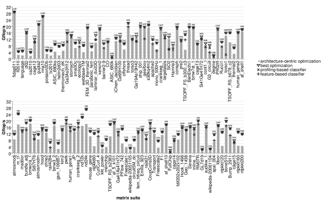
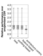
(a) Xeon Phi (224 threads)

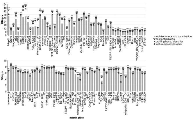
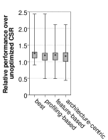
(b) Sandy Bridge-EP (32 threads)

Figure 2: Performance results of optimization selection on Xeon Phi and Sandy Bridge-EP. architecture-centric optimization refers to the optimization corresponding to the CMP class for Xeon Phi and MB class on Sandy Bridge-EP, while best optimization represents the maximum performance achieved with any of the tested optimizations (see Table 2).

On Xeon Phi, the importance of optimization selection is more prominent, providing an average speedup of $1.31\times$ with the profiling-based classifier and $1.30\times$ with the feature-based classifier, reaching $94.2\%$ and $93.5\%$ respectively of the best possible gain with the applied optimizations. This is mainly due to the architectural characteristics of the Xeon Phi coprocessor, which result in a quite balanced representation of each class. The coprocessor has a large amount of cores, which favor workload imbalance, and a very expensive (an order of magnitude bigger compared to multi-cores) cache miss latency, which further exposes irregularity in the accesses to the input vector. Thus, there are many matrices that exceed the LLC size and are not memory bandwidth bound. On the other hand, Sandy Bridge-EP is dominated by memory bandwidth bound matrices and can, therefore, only benefit from the correct classification of matrices belonging to minority classes. This makes higher accuracy rates more important on this architecture. Overall, our classifiers manage to optimize most of those matrices, leading to a $1.19\times$ and $1.20\times$ average speedup respectively and adding a 3% and 4% improvement over the architecture-centric optimization. Even though there are some misclassifications, they can be partially tolerated by the fact that the architecture-centric optimization can also be “harmful” for some matrices.

In total, the potential of an optimization selection approach for SpMV can be better estimated if we assume we have a “best” classifier, i.e., a classifier that always selects the best optimization presented in Figure 2, and compare it to an “architecture-centric” optimizer. In the box plots provided, we see that the “best” classifier improves SpMV performance over the “architecture-centric” by 37% on Xeon Phi and 9% on Sandy Bridge-EP on average.

It is important to point out that the achieved performance improvements presented in this work are limited by the optimizations we have selected. As this is not an actual optimization framework, we selected optimizations that can be easily implemented. Higher performance gains can be attained by a more elaborate examination of the wide variety of optimizations found in the literature and their association to our matrix classes. Selecting an even more suitable optimization after the matrix has been classified, based on its distinguishing structural features, is left for future work.

4.4 Runtime overhead

Our profiling-based optimization selection approach comprises two steps: running a number of micro-benchmarks on the input matrix and then applying our empirically-tuned classification algorithm to select the appropriate optimization. On the other hand, the online stage of the feature-based optimization selection methodology comes down to extracting the required features from the input matrix and then predicting its class using the pre-trained classifier.

	profiling-based	feature-based
Xeon Phi	462	14
Sandy Bridge-EP	462	16

Table 6: Average runtime overhead of optimization selection expressed in multi-threaded CSR-based SpMVs, using both classifiers presented in Section 3.2.

The runtime overhead of both classification approaches was measured in multithreaded CSR SpMV operations and is presented in Table 6, i.e., we report the ratio $\frac{T_{classification}}{T_{SpMV}}$, where $T_{classification}$ is the execution time of the classification and $T_{SpMV}$ the execution time of a single multithreaded SpMV operation. Apparently, the feature-based classifier has a significant advantage over its profiling-based alternative, as it requires only a couple dozen operations, which can be easily amortized in the context of an iterative numerical solver. We must note here that this overhead does not include any preprocessing required for applying an optimization. Among the optimizations applied in our evaluation, only the one for MB matrices requires preprocessing.

5 Related Work

Different sparse matrices have different sparsity patterns, and different architectures have different strengths and weaknesses. In order to achieve the best SpMV performance for the target sparse matrix on the target platform, an autotuning approach has long been considered to be beneficial. The first autotuning approaches attempted to tune parameters of specific sparse matrix storage formats. Towards this direction, the Optimized Sparse Kernel Interface (OSKI) library Vuduc et al. [2005] was developed as a collection of high performance sparse matrix operation primitives on single core processors. It relies on the SPARSITY framework Im et al. [2004] to tune the SpMV kernel, by applying multiple optimizations, including register blocking and cache blocking. Autotuning has also been used to find the best block and slice sizes of the input sparse matrix on modern CMPs and GPUs Choi et al. [2010].

There have been some research efforts closer to our work. The clSpMV framework Su and Keutzer [2012] is the first framework that analyzes the input sparse matrix at runtime, and recommends the best representation of the given sparse matrix, but it is restricted to GPU platforms. Towards the same direction, the authors in Guo et al. [2014] present an analytical and profile-based performance modeling to predict the execution time of SpMV on GPUs using different sparse matrix storage formats, in order the select the most efficient format for the target matrix. For each format under consideration, they establish a relationship between the number of nonzero elements per row in the matrix and the execution time of SpMV using that format, thus encapsulating to some degree the structure of the matrix in their methodology. Similarly, in Li et al. [2015], the authors propose a probabilistic model to estimate the execution time of SpMV on GPUs for different sparse matrix formats. They define a probability mass function to analyze the sparsity pattern of the target matrix and use it to estimate the compression efficiency of every format they examine. Combined with the hardware parameters of the GPU, they predict the performance of SpMV for every format. Since compression efficiency is the determinant factor in this approach, it is mainly targeted for memory bandwidth bound matrices. Closer to our approach is the SMAT autotuning framework Li et al. [2013]. This framework selects the most efficient format for the target matrix using feature parameters of the sparse matrix. It treats the format selection process as a classification problem, with each format under consideration representing a class, and leverages a data mining approach to generate a decision tree to perform the classification, based on the extracted feature parameters of the matrix. The distinguishing advantage of our optimization selection methodology over the aforementioned approaches, is that it decouples the decision making from specific optimizations, by predicting the major performance bottleneck of SpMV instead of SpMV execution time using a specific optimization. Thus, in contrary to the above frameworks, where incorporating a new optimization requires either retraining a model or defining a new one, our decision-making approach allows an autotuning framework to be easily extended, simply by assigning the new optimization to one of the classes.

6 Conclusions - Future Work

In this paper we presented a cross-platform methodology for optimizing the SpMV kernel and establish that, depending on the sparsity pattern of the matrix and the underlying architecture, a suitable optimization can be selected to improve SpMV performance. We formulate optimization selection for SpMV as a classification problem, with each class corresponding to a performance bottleneck. We first propose a profiling-based classifier, that relies on benchmarking the input matrix to perform the decision making. We also leverage machine learning to train Decision Tree and Naive Bayes classifiers that use comprehensive structural features to perform the classification and rely on the profiling-based classifier for the training process. Experimental evaluation on 115 sparse matrices and two platforms has demonstrated that our methodology is very promising, especially for the latest many-core architectures, which intensify various performance issues of the SpMV kernel.

Concerning future work, another direction that needs to be explored is whether a multi-level optimization approach would be beneficial for SpMV. It is very likely that, once the major performance issue of a matrix has been successfully addressed, another bottleneck will be exposed. Actually, the features that are extracted from the matrix and fed to our featured-based classifier can also be used in a following step to select even more targeted optimizations, depending solely on the sparsity pattern. We also intend to experiment with other machine learning techniques, in order to further improve the accuracy of our feature-based classifier. For example, semi-supervised learning, which allows some of the training data to be unlabeled, could be helpful, since there are matrices whose class cannot be easily determined. Finally, we plan to test our approach on GPU platforms.

References

- Agarwal et al. [1992] R. C. Agarwal, F. G. Gustavson, and M. Zubair. A high performance algorithm using pre-processing for the sparse matrix-vector multiplication. In Proceedings of the 1992 ACM/IEEE conference on Supercomputing, pages 32–41. IEEE Computer Society Press, 1992.
- Choi et al. [2010] J. W. Choi, A. Singh, and R. W. Vuduc. Model-driven autotuning of sparse matrix-vector multiply on gpus. In ACM Sigplan Notices, volume 45, pages 115–126. ACM, 2010.
- Cuthill and McKee [1969] E. Cuthill and J. McKee. Reducing the bandwidth of sparse symmetric matrices. In Proceedings of the 1969 24th national conference, pages 157–172. ACM, 1969.
- Dagum and Enon [1998] L. Dagum and R. Enon. Openmp: an industry standard api for shared-memory programming. Computational Science & Engineering, IEEE, 5(1):46–55, 1998.
- Davis and Hu [2011] T. A. Davis and Y. Hu. The university of florida sparse matrix collection. ACM Transactions on Mathematical Software (TOMS), 38(1):1, 2011.
- Geus and Röllin [1999] R. Geus and S. Röllin. Towards a fast parallel sparse matrix-vector multiplication. In PARCO, pages 308–315. World Scientific, 1999.
- Goumas et al. [2009] G. Goumas, K. Kourtis, N. Anastopoulos, V. Karakasis, and N. Koziris. Performance evaluation of the sparse matrix-vector multiplication on modern architectures. The Journal of Supercomputing, 50(1):36–77, 2009.
- Guo et al. [2014] P. Guo, L. Wang, and P. Chen. A performance modeling and optimization analysis tool for sparse matrix-vector multiplication on gpus. Parallel and Distributed Systems, IEEE Transactions on, 25(5):1112–1123, 2014.
- Im and Yelick [2001] E.-J. Im and K. Yelick. Optimizing sparse matrix computations for register reuse in sparsity. In Computational Science—ICCS 2001, pages 127–136. Springer, 2001.
- Im et al. [2004] E.-J. Im, K. Yelick, and R. Vuduc. Sparsity: Optimization framework for sparse matrix kernels. International Journal of High Performance Computing Applications, 18(1):135–158, 2004.
- Li et al. [2013] J. Li, G. Tan, M. Chen, and N. Sun. Smat: an input adaptive auto-tuner for sparse matrix-vector multiplication. In ACM SIGPLAN Notices, volume 48, pages 117–126. ACM, 2013.
- Li et al. [2015] K. Li, W. Yang, and K. Li. Performance analysis and optimization for spmv on gpu using probabilistic modeling. Parallel and Distributed Systems, IEEE Transactions on, 26(1):196–205, 2015.
- McCalpin [1995] J. D. McCalpin. Stream: Sustainable memory bandwidth in high performance computers, 1995.
- Mellor-Crummey and Garvin [2004] J. Mellor-Crummey and J. Garvin. Optimizing sparse matrix–vector product computations using unroll and jam. International Journal of High Performance Computing Applications, 18(2):225–236, 2004.
- Pichel et al. [2004] J. C. Pichel, D. B. Heras, J. C. Cabaleiro, and F. F. Rivera. Improving the locality of the sparse matrix-vector product on shared memory multiprocessors. In Parallel, Distributed and Network-Based Processing, 2004. Proceedings. 12th Euromicro Conference on, pages 66–71. IEEE, 2004.
- Pinar and Heath [1999] A. Pinar and M. T. Heath. Improving performance of sparse matrix-vector multiplication. In Proceedings of the 1999 ACM/IEEE conference on Supercomputing, page 30. ACM, 1999.
- Pooch and Nieder [1973] U. W. Pooch and A. Nieder. A survey of indexing techniques for sparse matrices. ACM Computing Surveys (CSUR), 5(2):109–133, 1973.
- Saad [1992] Y. Saad. Numerical methods for large eigenvalue problems, volume 158. SIAM, 1992.
- Su and Keutzer [2012] B.-Y. Su and K. Keutzer. clspmv: A cross-platform opencl spmv framework on gpus. In Proceedings of the 26th ACM international conference on Supercomputing, pages 353–364. ACM, 2012.
- Temam and Jalby [1992] O. Temam and W. Jalby. Characterizing the behavior of sparse algorithms on caches. In Proceedings of the 1992 ACM/IEEE conference on Supercomputing, pages 578–587. IEEE Computer Society Press, 1992.
- Toledo [1997] S. Toledo. Improving the memory-system performance of sparse-matrix vector multiplication. IBM Journal of research and development, 41(6):711–725, 1997.
- Vuduc et al. [2005] R. Vuduc, J. W. Demmel, and K. A. Yelick. Oski: A library of automatically tuned sparse matrix kernels. In Journal of Physics: Conference Series, volume 16, page 521. IOP Publishing, 2005.
- Vuduc and Moon [2005] R. W. Vuduc and H.-J. Moon. Fast sparse matrix-vector multiplication by exploiting variable block structure. In High Performance Computing and Communications, pages 807–816. Springer, 2005.
- Willcock and Lumsdaine [2006] J. Willcock and A. Lumsdaine. Accelerating sparse matrix computations via data compression. In Proceedings of the 20th annual international conference on Supercomputing, pages 307–316. ACM, 2006.