Bayesian recursive data pattern tomography

Abstract

We present a simple and efficient Bayesian recursive algorithm for the data-pattern scheme for quantum state reconstruction, which is applicable to situations where measurement settings can be controllably varied efficiently. The algorithm predicts the best measurements required to accurately reconstruct the unknown signal state in terms of a fixed set of probe states. In each iterative step, this algorithm seeks the measurement setting that minimizes the variance of the data-pattern estimator, which essentially measures the reconstruction accuracy, with the help of a data-pattern bank that was acquired prior to the signal reconstruction. We show that with this algorithm, it is possible to minimize the number of measurement settings required to obtain a reasonably accurate state estimator by using just the optimal settings and, at the same time, increasing the numerical efficiency of the data-pattern reconstruction.

I Introduction

In very general terms, quantum tomography involves a comprehensive toolset that allows an observer to carry out verification and diagnostics on quantum degrees of freedom. With it, the observer is able to acquire maximal information about a quantum source by characterizing its quantum state (quantum state tomography QST1 ; QST2 ; QST3 ). To perform this task, one usually needs a rather precisely calibrated measurement set-up. Calibrating a detection device for signals on an intensity level of a few quanta can be a challenge. In general, measurement schemes are lossy and noisy. For example, the so-called single-photon detectors are only able to distinguish between the presence and absence of a signal pulse (hence the alternative names “bucket” or “on/off” detectors). In addition, these detectors have wavelength-dependent efficiencies that are less-than-unity, and give dark photon counts in the presence of noise that may originate from either thermal fluctuation, afterpulsing for heterostructural detectors and other sources. The dead times incurred from minimizing such spurious counts further complicate photodetection. Precise calibration of measurement apparatuses (quantum process or detector tomography) is yet another well-established area in quantum tomography. More sophisticated device-calibration methods would generally entail the utilization of intrinsic quantum resources such as entanglement. Examples of such approaches include the “absolute calibration” method klyshko80 ; sergienko81 , and “self-testing” or “blind tomography” scarani ; Navascues . Quite often, device calibrations are carried out up to some experimental error uncertainties that are difficult to control. There are situations where detector calibration is impractical. For example, in wavefront sensing experiments wavefront , wavefront detectors that contain microlenses are practically impossible to calibrate reliably as they are, for close proximities between pairs of microlenses would result in calibration interference.

In this article, we discuss a particular tomography procedure that permits one to circumvent the need for measurement-device calibration when reconstructing the quantum state of any arbitrary signal — the data pattern tomography procedure proposed in 2010 data patterns 2010 . The idea is somewhat similar to that of optical image analysis with known optical response function classic . An observer measures responses (the data patterns, so to speak) for a set of known quantum probe states. Then, the observer matches them with the response obtained from the unknown signal of interest. This method is naturally insensitive to imperfections of the measurement set-up, since all device imperfections are automatically incorporated into and accounted for by the measured data patterns. This procedure can also be understood, in terms of reconstruction-subspace optimization, as a search for the optimal state estimator over the subspace that is spanned by the probe states.

The data-pattern scheme with coherent states as probe states was recently realized by the experimental groups in Oxford oxford and Paderborn paderborn for the reconstruction of few-photon states (thermal, heralded single-photon and two-photon states). It was shown that the data-pattern scheme is indeed feasible and is able to perform robust and accurate state reconstruction. At present, however, the procedure of data pattern inference is still far from optimal. In experiments oxford ; paderborn the reconstruction was done by considering only a set of probe states that was deemed sufficiently large (48 in Ref. oxford , 50-150 in Ref. paderborn ). One should understand that the choices of these “sufficiently large” numbers are not entirely ad hoc, as these choices are not based solely on the average number of photons in the signal, which can be inaccurate.

It is possible to estimate this “sufficiently large number” fairly accurately by making an educated guess of a class of plausible signal states that would closely describe the quantum source and choose a probe-state basis that best fits this class of states. In the language of statistics, this is equivalent to developing a useful prior for the data-pattern experiment. If the observer, after some rough preliminary calibration of the source, has reasons to believe that the unknown signal state is very likely residing in some operator subspace, he can make use of this insight to define the set of probe states that spans this subspace data patterns 2013 ; oxford ; spiral for data-pattern reconstruction data patterns 2010 ; data patterns 2013 .

From this pre-selected set of probe states and some fixed choice of measurement settings (or measurements in short), it is possible to optimize the inference procedure by incorporating more probe states from this search space to enhance the data-pattern fit. In this sense, a new and improved data-pattern fit is obtained by acquiring some more data patterns and incorporating them to the previous fit. However, if the optimization of the data-pattern fit is restricted to a fixed set of measurements, it may turn out that many of the pre-chosen probe states play little role in enhancing the fit. One such example would be the case of single-photon state inference in Ref. data patterns 2013 . In this report, approximately a third of the measured probe states practically give no constructive contributions to the final data-pattern fit in terms of reconstruction accuracy.

In the light of this finding, we propose an alternative methodology to optimize the data-pattern scheme. For situations in which adjusting measurement settings can be done quite precisely and efficiently in a well-controlled manner, we consider ways to optimally choose measurements for the signal state to provide the best fit for the given set of probe states. Since the probe states that collectively give a faithful description of the signal state can always be reasonably restricted to a finite number by some physical considerations of the source that allows the observer to truncate its dimension, one can optimize the subsequent measurements for a pre-chosen set of probe states with the aim of optimally utilizing these data patterns in order to increase the reconstruction accuracy.

Prior to the signal reconstruction, data patterns for the probe states are measured for various measurement settings and the subset of optimal settings for the signal reconstruction are directly determined from these patterns with a recursive numerical algorithm. In this way, the number of patterns to be used for signal reconstruction is minimized and numerical reconstruction can hence be carried out efficiently. With this same bank of data patterns, the observer can perform the same measurement optimization for other signal states for which these pre-chosen probe states are appropriate for their reconstruction.

For this purpose, we shall develop an efficient recursive Bayesian iterative procedure for the measurement optimization. The observer, with access to the data-pattern bank, can make use of this procedure to generate a sequence of optimal measurement settings that minimizes the reconstruction accuracy, and finally terminate this sequence after a natural stopping criterion is met. As a rule, when the reconstruction accuracy of the state estimator becomes comparable with the improvement of the data-pattern fit, it is then no longer necessary to perform any more measurement. Incorporating more data patterns from any other measurement will not lead to any appreciable increase in accuracy rosett ; enk ; moroder ; mogilevtsev2013 .

The outline of the article is as follows. In Sec. II, the basic elements of the recursive procedure is introduced. Next, we describe approximations that are valid for the data-pattern scheme for coping with the complexities of calculating Bayesian integrals and derive the expressions for the Bayesian update that is employed in the procedure in Sec. III. Following which, in Sec. IV, we shall formally discuss the measurement optimization procedure based on the Bayesian-update equations that were established in Sec. III, and its stopping criterion. Last, but not the least, in Sec. V, the mechanisms and results of this Bayesian numerical procedure are illustrated with some examples of low-intensity signal states with the help of probe coherent states.

II Basics

To lay the groundwork for subsequent discussions, let us outline the general scheme of things. We assume that there is a finite set of available probe states described by the density operators $\rho_{m}$, where $m=1\ldots M$. We would like to reconstruct the true signal state described by the density operator $\rho$, which is known, to some level of confidence after a preliminary calibration of the source, to be representable as a linear combination of these probe states,

$$\rho=\sum_{m=1}^{M}c^{\text{(true)}}_{m}\rho_{m},$$ (1)

where $c^{\text{(true)}}_{m}$ are real coefficients. The aim of the data-pattern inference procedure is to optimize these coefficients. To this end, we suppose that the experimental set-up allows us to vary measurement settings in a controlled and efficient manner, thereby allowing us to sequentially carry out different measurements on the source to obtain data patterns. Out of a total number of $K$ measurement settings employed, the $k$th setting yields one of two outcomes described by the positive operators $\Pi_{k}$ and $1-\Pi_{k}$ that compose a positive operator-valued measure (POVM) for this measurement. The probability of the outcome $\Pi_{k}$ for the $k$th measurement performed on the signal state is given by Born’s rule as

$$P_{k}=\mathrm{Tr}\{\Pi_{k}\rho\}=\sum_{m=1}^{M}c^{\text{(true)}}_{m}p_{km}=\sum_{m=1}^{M}c^{\text{(true)}}_{m}\mathrm{Tr}\{\Pi_{k}\rho_{m}\}$$ (2)

where $p_{km}$ is the probability for the measurement outcome $\Pi_{k}$ and the $m$th probe state. In practice, we have access to a finite number of signal and probe copies, say, $N$ each for every measurement. So, instead of probabilities $P_{k}$ and $p_{km}$, one measures frequencies $F_{k}$ and $f_{km}$, which are respectively the so-called data patterns for the signal state and the probe states data patterns 2010 ; data patterns 2013 ; spiral ; oxford ; paderborn . The goal of the data-pattern reconstruction scheme is to find the estimated coefficients $c_{m}$ that give the closest match between the signal patterns {$F_{k}$} and the probe patterns {$f_{km}$}. In all previous studies on the data-pattern scheme, this matching (or fitting) was done with least-squares inversion by minimising the squared distance

$$D=\sum\limits_{k=1}^{M}\left(F_{k}-\sum_{m=1}^{M}c_{m}f_{km}\right)^{2}$$ (3)

for the estimated coefficients $c_{m}$. We need a positive semidefinite state estimator $\rho_{\text{est}}\geq 0$ that is of unit trace, where the latter linear constraint can be straightforwardly imposed with a parametrization involving $M-1$ independent coefficients, such that $c_{M}=1-\sum_{m=1}^{M-1}c_{m}$. Different versions of least-squares inversion that account for the positivity constraint and other general linear constraints were used for data-pattern matching data patterns 2010 ; data patterns 2013 ). Efficient inference procedure that directly incorporates the positivity constraint in the search algorithm that improves the data pattern fit by accumulating more data patterns from a pre-chosen set was also established in Ref. spiral .

With the basic mathematical formalism now in place, one can understand why it is generally unnecessary to accumulate a huge dataset from many measurement settings to reconstruct unknown signals. For instance, in the idealized hypothetical situation where statistical fluctuation is absent, if the signal state is any one of the probe states, say $\rho=\rho_{m=m_{0}}$, then one measurement setting ($\Pi_{1}$) is enough to determine the state since one of the probe patterns $f_{1m_{0}}$ would precisely match the signal data pattern $F_{1}$. All other probe patterns give nonzero differences with $F_{1}$. This simple intuition suggests that in a realistic scenario where statistical fluctuation is present, if the unknown signal state is a linear combination of a few of the probe states, there should exist a numerical method to systematically search for a small set of optimized measurement settings that would typically be much less than the total number of probe states considered. This significant reduction in the total number $K$ of optimal measurement settings required would also greatly enhance the numerical efficiencies in reconstructing the state. In the discussions to come, for a fixed set of probe states, we shall derive a recursive iterative algorithm that decisively selects optimal measurement settings in a sequential manner using Bayesian statistical reasonings for finite data.

To choose optimal measurements sequentially, we shall introduce a numerical procedure that invokes an iterative Bayesian-update routine on the probability distribution for the state estimator that is a function of the coefficients $c_{m}$. The observer would start with a large bank of data patterns that are acquired through different measurement settings prior to the signal reconstruction. Since all information about the measurement set-up is encoded in the data patterns, the frequencies of the measurement outcomes, along with any existing systematic errors, for the unknown signal state are also encoded in its data patterns $F_{k}$. As this iterative algorithm looks for optimal solutions by inferring from data patterns, all systematic errors are automatically accounted for.

Let us discuss the essential elements for the iterative algorithm. After collecting data for $k$ measurement settings, the corresponding posterior probability distribution $w\left(\mathbf{c}\,|\mathbf{F}^{(k)}\right)$ describes the distribution of the column of coefficients $\mathbf{c}=(c_{1}\ldots c_{M-1})^{\textsc{T}}$, conditioned on the signal data patterns $\mathbf{F}^{(k)}=(F_{1}\ldots F_{k})^{\textsc{T}}$ obtained with $k$ different measurements. Performing an additional measurement of a different setting enlarges the set of data patterns for the signal. Consequently, the updated posterior distribution is

$$\begin{aligned} w\left(\mathbf{c}\,\Big{|}\mathbf{F}^{(k+1)}\right)=\frac{w\left(\mathbf{c}\,\Big{|}\mathbf{F}^{(k)}\right)[P_{k+1}(\mathbf{c})]^{NF_{k+1}}\left[1-P_{k+1}(\mathbf{c})\right]^{N(1-F_{k+1})}}{\int d\mathbf{c}\,w\left(\mathbf{c}\,\Big{|}\mathbf{F}^{(k)}\right)[P_{k+1}(\mathbf{c})]^{NF_{k+1}}\left[1-P_{k+1}(\mathbf{c})\right]^{N(1-F_{k+1})}},\end{aligned}$$ (4)

where the estimated probability for the $k$th measurement setting reads

$$P_{{k}}(\mathbf{c})\approx\sum_{m=1}^{M-1}c_{m}f_{{k}m}+\left(1-\sum_{m=1}^{M-1}c_{m}\right)f_{kM},$$ (5)

the integration measure is given by

$$d\mathbf{c}=\prod\limits_{m=1}^{M-1}dc_{m},$$

and $N$ is the number of signal-state copies used for each measurement setting. The integration in the denominator of Eq. (4) is carried out over the region $\Omega_{c}$ of coefficients $c_{m}$ where the estimator for $\rho$ in (1) is positive semidefinite.

III Quantum complexities in Bayesian reasoning

Generally, performing Bayesian updates for an unknown state characterized by a large number of state parameters is computationally demanding, since it involves calculating operator integrals over the region of admissible parameter values. (In our context, the denominator in Eq. (4).) This region is defined by the positivity constraint of the state estimator, $\rho_{\text{est}}\geq 0$, with the boundary representing rank-deficient states. To estimate the integral in Eq. (4), a number of statistical Monte-Carlo methods were suggested and implemented (see, for example, robin2010 and the relevant references therein). Incidently, the Bayesian procedure for choosing the measurements depending on the collected data was proposed in Ref. husar . This procedure also involves a statistical sampling method (sequential importance sampling douche ) that still does not effectively sample the state space according to the required posterior distribution. Only recently, a more efficient and direct Monte-Carlo approach that invokes Hamiltonian statistical methods to sample the state space according to any given arbitrary posterior distribution was introduced in Ref. berge . Despite this breakthrough, while this approach is efficient for single- and two-qubit cases, Hamiltonian Monte-Carlo sampling for Hilbert spaces of larger dimensions remains to be a relatively formidable task that requires more computational resources and a cleverer operator-space parametrization. For practical purposes, we shall henceforth adopt a much simpler and far more computationally efficient approximation that is similar to Kalman filtering (see kalman and the relevant references therein). As it will be seen below, it follows naturally from the specifications of the data-pattern reconstruction scheme.

First, let us outline some reasonable and useful approximations that are in accordance with the specifications of the data-pattern scheme. For a finite number of state copies $N$, the probe patterns $f_{km}$ are random variables. We shall assume that $N$ is sufficiently large, so that the maximum of the (Gaussian-approximated) posterior distribution $w\left(\mathbf{c},|\mathbf{F}^{(k)}\right)$ corresponds to a positive semidefinite $\rho$. This assumption is justified when the signal state is inside the state space (full rank) — the real situation in practice — and its consideration in practical implementations of the data-pattern reconstruction scheme on quantum states of the electromagnetic field can be appreciated in oxford ; paderborn . Measuring large samples of quantum systems in these experimental situations is typically not a very resource-intensive task.

Next, we proceed, in the spirit of Kalman filtering, to approximate the posterior distribution $w\left(\mathbf{c},|\mathbf{F}^{(k)}\right)$ with a Gaussian distribution of a data-dependent mean and variance (see Refs. kalman and robin2010 ). Thus, assuming the uninformative uniform prior distribution in the $\{c_{m}\}$-space, we arrive at the following simplified form of Eq. (4):

$$w\left(\mathbf{c}\,\Big{|}\mathbf{F}^{(k+1)}\right){\propto}\,w\left(\mathbf{c}\,\Big{|}\mathbf{F}^{(k)}\right)\exp\left(-\sum_{m,n=1}^{M-1}\frac{[f_{k+1,m}-f_{k+1,M}][f_{k+1,n}-f_{k+1,M})]}{2\sigma_{k+1}^{2}}c_{m}c_{n}\right)$$ (6)

$$\times\exp\left(\sum_{m=1}^{M-1}\frac{[\mu_{k+1}-f_{k+1,M}][f_{k+1,m}-f_{k+1,M}]}{\sigma_{k+1}^{2}}c_{m}\right),$$

where

$$\sigma_{k+1}^{2}=\frac{(NF_{k+1})(N(1-F_{k+1})+1)}{(N+2)^{2}(N+3)},$$ (7)

$$\mu_{k+1}=\frac{NF_{k+1}+1}{N+2}.$$

Here, Eq. (5) is used for evaluating $P_{k+1}(\mathbf{c})$.

Notice that one can cope with a posterior distribution extending outside the state space by using the procedure outlined in Ref. kalman . The procedure involves calculating the mean and variance for only the truncated posterior distribution of Eq. (6) that lies in the state space, and redefine the posterior distribution in the next step of the iteration to be the Gaussian distribution having these distribution parameters, so that no more than a very small portion of the updated posterior distribution extends outside the physically allowed space, or

$$\int_{\begin{subarray}{c}\text{outside the}\\ \text{state space}\end{subarray}}d\mathbf{c}\,w\left(\mathbf{c}\,\Big{|}\mathbf{F}^{(k)}\right)\leq\epsilon$$ (8)

for some $0<\epsilon\ll 1$. More details are given in the Appendix.

IV Choosing optimal measurement settings

To optimally select the appropriate subset of measurement settings out of all the choices that were used to accumulate the bank of data patterns prior for signal reconstruction, a recursive scheme to choose the next measurement setting according to the previously used settings and a suitable criterion for terminating this scheme are in order.

To set the stage for implementing the algorithm, we first specify that in this article, we shall take the mean squared error

$$\Delta_{\rho}^{2}=\sum^{M-1}_{m=1}\left<\left(c_{m}-c^{(\text{true})}_{m}+\{\text{noise}\}\right)^{2}\right>_{w}$$ (9)

to be the measure of the (averaged) reconstruction accuracy of the state estimator $\rho_{\text{est}}=\sum_{m}c_{m}\rho_{m}$ relative to the true signal state $\rho$, where $\langle c_{m}\rangle_{w}=\int d\mathbf{c}\;w\left(\mathbf{c}\,\Big{|}\mathbf{F}^{(k)}\right)c_{m}$ is the mean with respect to the posterior distribution of the $c_{m}$s and {noise} refers to an unbiased random perturbation on the signal state $\rho$. Expanding the right-hand side gives

$$\Delta_{\rho}^{2}=\mathrm{Bias}[\{c_{m}\}]+\mathrm{Var}[\{c_{m}\}]+\sigma^{2}_{\mathrm{noise}}\,,$$ (10)

where the magnitude of the bias term

$$\mathrm{Bias}[\{c_{m}\}]=\sum^{M-1}_{m=1}\left(\langle c_{m}\rangle_{w}-c^{(\text{true})}_{m}\right)^{2}$$ (11)

depends on the choice of reconstruction scheme for translating measurement data to a quantum state and the magnitude of experimental systematic errors. The size of $\sigma^{2}_{\mathrm{noise}}$ depends on the random environmental noise. Since we shall only consider, in the hypothetical absence of the positivity constraint and systematic errors, estimators $\rho_{\text{est}}$s that are generated from the data in an unbiased way $\left(\langle c_{m}\rangle_{w}=c^{(\text{true})}_{m}\right)$, the bias term becomes insignificant in the situation of large $N$, negligible systematic errors and realistic sources described by full-rank signal states, albeit very close to the boundary for practical quantum protocols. The noise variance also vanishes when the source is relatively well stabilized. As a result, only the variance term

$$\mathrm{Var}[\{c_{m}\}]=\sum^{M-1}_{m=1}\left<(c_{m}-\left<c_{m}\right>_{w})^{2}\right>_{w}$$ (12)

is relevant in determining the estimator’s accuracy. One can thus appreciate that when changes in the variance for each subsequent iterative step become smaller than the variance itself, then carrying out these subsequent steps by incorporating additional measurement settings into the reconstruction will not improve the reconstruction accuracy.

In view of the above reasoning, the natural figure of merit that reflects our knowledge about the investigated unknown signal state during the $k$th step of the iterative procedure, as a function of $w\left(\mathbf{c}\,\Big{|}\mathbf{F}^{(k)}\right)$, would be the coefficient variance:

$$\operatorname{Var}(\mathbf{c}|w,k) \equiv{\mathrm{Var}[\{c_{m}\}]}$$

$$=\sum_{m=1}^{M-1}\left\langle\left(c_{m}-\langle c_{m}\rangle_{w}\right)^{2}\right\rangle_{w}$$ (13)

$$=\int d\mathbf{c}\;w\left(\mathbf{c}\,\Big{|}\mathbf{F}^{(k)}\right)\sum_{m=1}^{M-1}(c_{m}-\langle c_{m}\rangle_{w})^{2}.$$

The estimated information gained by incorporating the $(k+1)$th measurement is therefore manifested as a decrease in the coefficient variance for this measurement. The predicted average variance after the ($k+1$)th measurement is then given by the average over all possible data of a given $N$:

$$\langle\operatorname{Var}(\mathbf{c}|\Pi_{k+1})\rangle=\sum_{n=0}^{N}p\left\{w;n,k\right\}\times\;$$ (14)

$$\operatorname{Var}(\mathbf{c}|w,k+1;F_{k+1}=n/N),$$

where $p\left\{w;n{,k}\right\}$ is the probability of obtaining $n$ successful outcomes of $\Pi_{k+1}$; $\operatorname{Var}(\mathbf{c}|w,k+1;F_{k+1}=n/N)$ is calculated from Eq. (IV) for $\mathbf{F}^{(k+1)}=(F_{1},\ldots,F_{k},F_{k+1}=n/N)$ (thus, all possible measured frequencies $F_{k+1}=0,1/N,\ldots,1$ are included in average variance estimation). This probability is estimated based on the previous posterior distribution $w\left(\mathbf{c}\,\Big{|}\mathbf{F}^{(k)}\right)$:

$$p\left\{w;n{,k}\right\}$$ (15)

$$= \int d\mathbf{c}\;\binom{N}{n}[P_{k+1}(\mathbf{c})]^{n}\left[1-P_{k+1}(\mathbf{c})\right]^{N-n}w\left(\mathbf{c}\,\Big{|}\mathbf{F}^{(k)}\right).$$

So, according to our prescription, for the ($k+1$)th step of the iterative update procedure, the observer should choose the measurement setting that minimizes the predicted average variance, that is one should look for

$$\Delta_{k+1}=\min_{\begin{subarray}{c}\text{all available}\\ \text{settings}\end{subarray}}\Big{\{}\langle\operatorname{Var}(\mathbf{c}|\Pi_{k+1})\rangle\Big{\}},$$ (16)

where the minimum is carried out over all measurement settings from the data-pattern bank. Hence, the criterion for terminating the iteration is when the decrease in the predicted variance is much less than the variance itself,

$$|\Delta_{k+1}-\operatorname{Var}(\mathbf{c}|w,k)|\ll\operatorname{Var}(\mathbf{c}|w,k),$$ (17)

where $\Delta_{k+1}$ is given by Eq. (16).

One can surmise that for some signal states (for example, the probe states themselves) only a few iterative steps (measurements on the signal) would be sufficient to obtain a good fit of the posterior distribution. In the preceding section, we shall demonstrate that this is indeed the case for various kinds of signals.

We close this section by reiterating that it is possible to technically cope with the numerical iteration even when the tails of the posterior distribution typically extends to regions outside the state space. One can improve on the final estimation of the posterior distribution by truncating the part outside the state space, followed by a Gaussian refitting. If the change in the variance becomes negligible, then approximating the correct posterior distribution with a function that extends outside the state space will not lead to any appreciable difference as far as signal reconstruction is concerned.

V Discussions & examples

In this section, we illustrate the mechanisms and results of the full recursive data-pattern tomography scheme. To this end, we shall specify the set of probe states and measurements for this scheme.

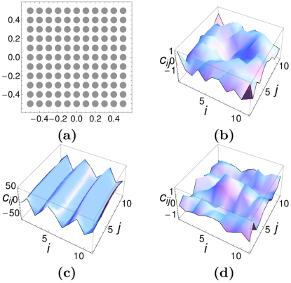
Figure 1: (Color online) (a) The lattice of probe coherent states in phase-space representation, indicated by an array of gray filled circles. The abscissa represents the real part of the complex amplitude that defines the phase space, whereas the ordinate represents the imaginary part. (b) Coefficients $c_{m}$ for the single-photon signal. (c) Coefficients $c_{m}$ for the signal coherent state with an amplitude $\alpha=1$ which magnitude is larger than the lattice width. (d) Coefficients $c_{m}$ for the signal even coherent state, $|\psi\rangle\propto|\alpha=0.5\rangle+|\alpha=-0.5\rangle$. Indices $i,j$ label the points on the lattice in panel (a); $i$ labels the abscissa starting from the lower-left corner, $j$ labels the ordinate starting from the lower-left corner.

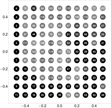
Figure 2: Simulation of the reconstruction process for the coherent state of amplitude $\alpha=0.5$, which is one of the probe states employed. Phase-space representation of all available measurement settings, where the lattice circles in Fig. 1(a) are replaced by filled numbered circles to display the sequence of optimal measurement settings as chosen by the recursive Bayesian algorithm. Black circles represent measurement-optimization stages before the stopping criterion is satisfied, and circles of shades of gray represent stages after the criterion is satisfied, with the lightest shade indicating the smallest change in reconstruction accuracy relative to the preceding step.

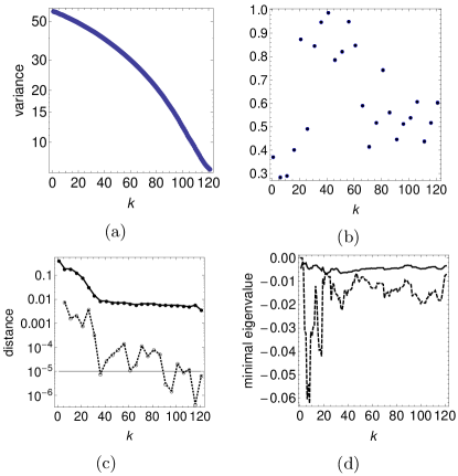
Figure 3: (Color online) Simulation of the reconstruction process for the coherent state of amplitude $\alpha=0.5$, which is one of the probe states employed. (a) Plot of the variance $\langle\operatorname{Var}(\mathbf{c}|\Pi_{k})\rangle$ against the iterative step number or the optimal setting label. (b) Reconstructed probabilities of measurement settings for the state estimator (filled circle) in the last step of the Bayesian iteration (blue empty circles) and the corresponding measured frequencies (black filled circles that are connected to the blue ones, both types of which in this case are close to each other). (c) Distance between the true state and its estimator averaged over the posterior distribution (solid lines and filled circles); distance between estimated signal states (averaged over the posterior distribution) for the $k$th and $(k+1)$th iterative steps (dotted line and empty circles). The number of copies per measurement setting is $N=1000$ for all probe and signal states. (d) The minimal eigenvalues for the estimators before (dotted line) and after shearing-refitting (solid line) for the $k$th iterative step.

V.1 Probe states

For practical purposes, it is advisable to use probe states that can be easily generated in the laboratory, and provide an accurate and computationally manageable representation of the unknown signal state. In previous works on the data-pattern scheme, it was shown that the usual coherent states satisfy these practical requirements rather well. One can routinely generate a large set of coherent states that can potentially provide accurate representations for a wide class of signal states data patterns 2010 ; data patterns 2013 . Apart from coherent states, one can also take a general set of Gaussian states as suitable candidates for the probe states. An example would be a set of thermal mixtures of coherent states. Interestingly, it has been shown that the inclusion of just one such thermal state in the set of probe states involving other Gaussian states can lead to a significant reduction in the number of probe states required to accurately represent some signal states data patterns 2013 .

To proceed we consider a set of probe coherent states that defines a square lattice that is centered at the origin of the two-dimensional phase space (see Fig. 1(a)). Without loss of generality, we limit ourselves to signal states that are characterized by small amplitudes in phase space. For the subsequent simulation examples, we consider three different signal states: the coherent state with amplitude $\alpha=1$, the single-photon Fock state, and the even coherent state of amplitude $\alpha=0.5$, that is the superposition $|\psi\rangle\propto|\alpha=0.5\rangle+|\alpha=-0.5\rangle$. Figures 1(b) through 1(d) illustrate these three signal states in phase space. With this set of probe states, the optimal fitting for all three signal states respectively give the operators $\rho$ that have essentially 100% fidelity with the signal states, which are exemplifying indications that our chosen probe-coherent-state basis can reliably represent a wide class of signal states.

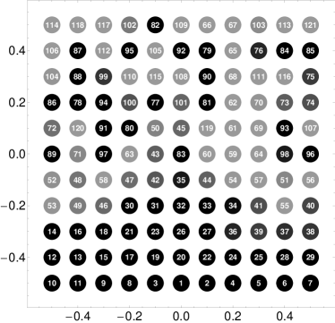
Figure 4: Simulation of the reconstruction process for the single-photon state. See Fig. 2 for the description of the figure.

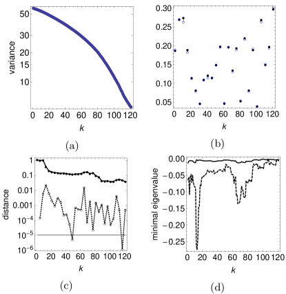
Figure 5: (Color online) Simulation of the reconstruction process for the single-photon state. See Fig. 3 for the descriptions of all figure panels.

V.2 Phase-Space Sampling

As a means of showcasing the mechanism of our recursive Bayesian method in the simplest and most straightforward way, let us take the intended measurements to be projections onto coherent states, so that the $k$th measurement is described by observing a coherent-state outcome $\Pi_{k}=|\beta_{k}\rangle\langle\beta_{k}|$ of some chosen complex amplitude $\beta_{k}$. A collection of these measurement projections define the scope of the two-dimensional phase space that is sampled by these measurements. For the assumed ideal lossless detection, the probability of observing the $k$th coherent-state outcome given a probe state $\rho_{m}$ is given by

$$p_{km}=\langle\beta_{k}|\rho_{m}|\beta_{k}\rangle=\exp\!\left(-|\alpha_{m}-\beta_{k}|^{2}\right),$$ (18)

where $\alpha_{m}$ denotes the complex amplitude of the probe coherent state. Deterministic sampling of the phase space is achievable experimentally using the unbalanced homodyne technique unb_homo1 ; unb_homo2 and has, for instance, been applied to wave-function reconstruction via phase retrieval unb_homo3 and Bell-inequality testing unb_homo4 . For non-ideal detection, this method of systematically sampling the phase space has been demonstrated experimentally paris .

For numerical experiments simulated with Monte Carlo techniques, the probabilities of respectively observing every coherent-state setting $k$ for the $m$th probe state are measured with a finite number of state copies $N_{\text{p}}$. The frequencies are taken as the probe patterns. Amplitudes of the probe states are selected as equidistant phase-space points that form a square lattice (see Fig. 1(a), for instance). Note that the matrix of the probabilities $p_{km}$ is generally not square. Typically, the number of employed measurement settings $K$ is not equal to the number of probe states $M$, and the sets of amplitudes {$\alpha_{m}$} and {$\beta_{k}$} may not even be overlapping in the sense that $\alpha_{m}\neq\beta_{k}$ for all $k$ and $m$. However, for the sake of simplicity we let $M=K$ and $\alpha_{m}=\beta_{m}$. We also assume that the signal is measured for a finite number of state copies $N_{\text{s}}$ per measurement setting such that $N_{\text{p}}=N_{\text{s}}=N$. Prior to the reconstruction, the probe-pattern bank was obtained by simulating all the projections on the phase-space lattice for every probe state with $N=1000$ copies.

V.3 Results

We are now ready to demonstrate that the recursive Bayesian iterative algorithm defined in Sec. IV can significantly reduce the number of optimal measurements needed for a faithful reconstruction of the signal state. For this purpose, we take the signal state to be one of the probe coherent state with amplitude 0.5. Figures 2 and 3 illustrate aspects of a simulation conducted with 121 probe states residing in the $11\times 11$ phase-space square lattice (see Fig. 2), which is also the same lattice illustrating the measurement settings. Figure 2 highlights the sequence of optimal measurement settings dictated by the recursive Bayesian algorithm as phase-space trajectories (indicated by integers in filled circles). The evolution phase-space trajectory is self-explanatorily indicated by the numbered circles. Figure 3(a) gives the plot of total variance of the posterior distribution, $\langle\operatorname{Var}(\mathbf{c}|\Pi_{k})\rangle$, against the iterative step number (with 121 being the largest) or the optimal setting label. From Fig. 3(c), one can see that after measuring around 58 optimal measurement settings, the changes in the squared distances, defined by Eqs. (IV) and (14), become much smaller than the distances themselves, implying that no further improvements can be exploited. One can also look at the distance between estimated signal states (averaged over the posterior distribution) for the $k$th and $(k+1)$th optimal setting (dotted line in Fig. 3(c)). Figure 3(d) illustrates how the shearing-refitting procedure affects the minimal eigenvalue of the estimated signal state.

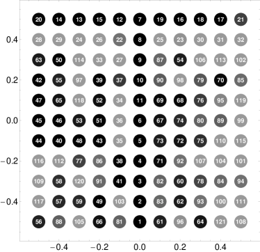
Figure 6: (Color online) Simulation of the reconstruction process for the even coherent state of amplitude $\alpha=0.5$. See Fig. 2 for the description of the figure.

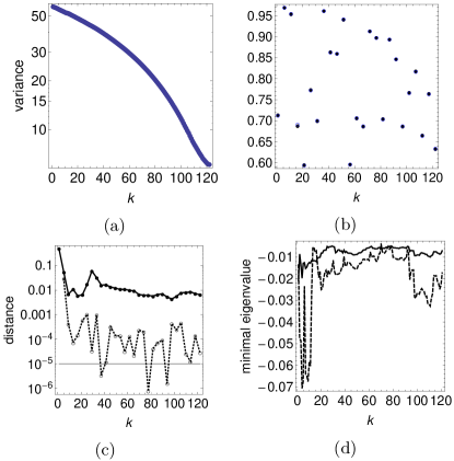
Figure 7: (Color online) Simulation of the reconstruction process for the single-photon state. See Fig. 3 for the descriptions of all figure panels.

Figures 4 and 5 show the simulated reconstruction process for a single-photon state, which is a nonclassical state having a highly singular Glauber–Sudarshan P function. All the typical features of the iterative procedure for the coherent-state signal are also present here. Again, the total number of optimal measurement settings employed is less than the number of parameters $M$ (Reading off from the panels (b) and (c), about $K=100$ measurement settings is sufficient for an accurate signal reconstruction). For the same $N$ value and stopping criterion, the reconstruction accuracy of the estimator for the coherent state is higher than that of the estimator for the single-photon state.

Figures 6 and 7 pertain to the reconstruction of another nonclassical state: the even coherent state $|\psi\rangle\propto|\alpha=0.5\rangle+|\alpha=-0.5\rangle$. One can see that, again, all the prominent features of the reconstruction procedure are the same as in the previous two examples. The number of optimal measurement settings needed (about $K=90$) is also less than the total number of parameters.

The reconstruction accuracy of the estimator for the even coherent state is higher than the single-photon state, as can be clearly seen by comparing the (b) panels in Figs. 5 and 7, where the estimated probabilities and measured frequencies are shown. On hindsight, it is to be expected that the single-photon state results in a less faithful representation in the coherent-state basis relative to the even (or odd) coherent state. The reason is that this state has a rather large classical component. An equal statistical mixture of just two coherent projectors of respectively $\left|\alpha=0.5\right>$ and $\left|\alpha=-0.5\right>$ would already give a rather high fidelity (0.8894).

We end this discussion by briefly summarizing the numerical technique that enforces the localization of the posterior distribution inside the admissible state-space. The update formulas (5) and (6) essentially specify a Gaussian distribution for the coefficient vector $\mathbf{c}$ without imposing the positivity restriction. In each iterative step of the reconstruction procedure, just before the estimation of the average variance, a corrected Gaussian distribution that localizes inside the state space is computed in the manner described in Ref. kalman .

To incorporate the positivity constraint for quantum states, we approximate the state space by a set of linear inequality constraints on the coefficient vector $\mathbf{c}=(c_{1}\,\,c_{2}\,\,\ldots\,\,c_{M-1})^{\textsc{T}}$. According to the definition of a quantum state, a density operator $\rho$ must satisfy the inequality $\left\langle{\Psi}\left|{\rho}\vphantom{\Psi}\right|\kern-1.2pt{\Psi}\right\rangle\geq 0$ for any ket $\left|{\Psi}\right\rangle$. In practice, we can only account for a finite set of inequality constraints $\left\langle{\Psi_{i}}\left|{\rho}\vphantom{\Psi_{i}}\right|\kern-1.2pt{\Psi_{i}}\right\rangle\geq 0$ defined by a finite set of test kets $\{|\Psi_{i}\rangle\}$. If this set of test kets is large enough, the finite set of inequalities provides a good approximation for the positivity constraint for operator $\rho$. It is worth noting, that if $\rho$ has a finite number of non-zero eigenvalues and the set of test kets includes all the eigenkets of $\rho$ corresponding to non-zero eigenvalues, the set of inequalities provide an exact description of the state space. In the examples above, the test-ket set includes the Fock states $|n\rangle$, with $n=0,\ldots,40$, and the probe coherent states. Equation (1) implies that the coefficients $c_{m}$ must satisfy the following inequalities

$$\sum_{m=1}^{M-1}c_{m}v_{m,i}\geq u_{i},$$ (19)

where $v_{m,i}=\left\langle{\Psi_{i}}\left|{\rho_{m}}\vphantom{\Psi_{i}}\right|\kern-1.2pt{\Psi_{i}}\right\rangle-\left\langle{\Psi_{i}}\left|{\rho_{M}}\vphantom{\Psi_{i}}\right|\kern-1.2pt{\Psi_{i}}\right\rangle$ and $u_{i}=-\left\langle{\Psi_{i}}\left|{\rho_{M}}\vphantom{\Psi_{i}}\right|\kern-1.2pt{\Psi_{i}}\right\rangle$, in order to satisfy the positivity constraint.

Appendix A describes the iterative procedure of distribution shearing of the initial posterior distribution with a significant portion extending outside the state space for a finite set of linear constraints, so that the final (Gaussian) posterior distribution extends outside the state space only minimally.

VI Conclusions

We have developed a simple and practical Bayesian procedure for enhancing the data-pattern reconstruction of signal states. The essence of the procedure is to sequentially choose the minimal set of optimal measurements needed to faithfully reconstruct the signal with a pre-chosen basis of probe states. In each step of the procedure, the measurement setting that minimizes the estimation error specified by the posterior distribution is incorporated into the previously measured settings. Upon consideration of specific features of the data-pattern scheme, we establish this recursive Bayesian procedure in the spirit of Kalman filtering. Such an approach allows us to handle large probe-state bases. We have demonstrated the mechanisms of our proposed Bayesian recursive data-pattern procedure with a set of more than one hundred probe coherent states to obtain accurate and efficient reconstruction of the coherent-state, single-photon-state and even-coherent-state signals. For some signal states, our recursive procedure even allows for accurate reconstruction using considerably less measurement settings than the elements of the probe-state basis used to represent the state. We expect that our scheme will be of much use in practical applications of data-pattern tomography.

VII Acknowledgments

A. M. and D. M. acknowledge the support of the National Academy of Sciences of Belarus through the program ”Convergence”, and FAPESP grant 2014/21188-0 (D. M.). Y. S. T., J. Ř., and Z. H. acknowledge the support of the Grant Agency of the Czech Republic (Grant No. 15-031945), the IGA Project of the Palacky University (Grant No. PRF 2015-002), and the European Union Seventh Framework Programme under Grant Agreement No. 308803 (Project BRISQ2).

Appendix A Distribution shearing and Gaussian refitting

The Gaussian posterior distribution can be parameterized as $w(\mathbf{c})\propto\exp\left(-\mathbf{c}\bm{\cdot}\mathbf{A}{\bm{\cdot}}\mathbf{c}+{\mathbf{b}}\bm{\cdot}\mathbf{c}\right)$, where $\mathbf{A}$ is an $(M-1)\times(M-1)$ matrix and ${\mathbf{b}}$ is a column vector with $(M-1)$ elements. For convenience, we introduce the new vectorial variable

$$\mathbf{c}^{\prime}=\mathbf{A}^{1/2}{\bm{\cdot}}\mathbf{c}-\frac{1}{2}\mathbf{A}^{-1/2}{\bm{\cdot}\mathbf{b}},$$ (20)

in which the expression for the posterior distribution simplifies immensely to $w(\mathbf{c}^{\prime})\propto\exp\left(-\mathbf{c}^{\prime}\bm{\cdot}\mathbf{c}^{\prime}\right)$. If the column $\mathbf{c}$ satisfies Eq. (19), then the new column $\mathbf{c}^{\prime}$ will satisfy a similar set of linear constraints $\mathbf{c}^{\prime}\bm{\cdot}\mathbf{v}_{i}^{\prime}\geq u_{i}^{\prime}$, where

$$\mathbf{v}_{i}^{\prime}=\mathbf{A}^{-1/2}{\bm{\cdot}}\mathbf{v}_{i},\;u_{i}^{\prime}=u_{i}-\frac{1}{2}\mathbf{v}_{i}\bm{\cdot}\mathbf{A}^{-1}{\bm{\cdot}}{\mathbf{b}}.$$ (21)

If we had only one constraint, say $\mathbf{c}^{\prime}\bm{\cdot}\mathbf{v}_{1}^{\prime}\geq u_{1}^{\prime}$, distribution shearing could be carried out in the following way. Owing to rotational symmetry of the Gaussian posterior distribution $w(\mathbf{c}^{\prime})$, only variations along the direction of $\mathbf{v}_{1}^{\prime}/\left|\mathbf{v}_{1}^{\prime}\right|$ matters. Upon introducing another variable $x=\mathbf{c}^{\prime}\bm{\cdot}\mathbf{v}_{1}^{\prime}/\left|\mathbf{v}_{1}^{\prime}\right|$, we consider the marginal distribution $w(x)\propto\exp(-x^{2})$ with the constraint $x\geq x_{0}=u_{1}^{\prime}/\left|\mathbf{v}_{1}^{\prime}\right|$. Hence, distribution shearing and Gaussian refitting would yield a new marginal distribution $\tilde{w}(x)\propto\exp\left(-(1+a)x^{2}+bx\right)$ of real coefficients $a$ and $b$ that gives the same mean value $\langle x\rangle$ for the physical portion of the initial distribution $w(x)$ inasmuch as

$$\frac{\int_{x_{0}}^{\infty}{dx}\,xw(x)}{\int_{x_{0}}^{\infty}{dx}\,w(x)}=\frac{\int_{x_{0}}^{\infty}{dx}\,x\tilde{w}(x)}{\int_{x_{0}}^{\infty}{dx}\,\tilde{w}(x)},$$ (22)

but with a smaller probability

$$p=\int_{-\infty}^{x_{0}}{dx}\,\tilde{w}(x)$$ (23)

of the variable $x$ lying outside the physical region that is defined by its linear constraint. After some straightforward evaluations of the integrals in Eqs. (22) and (23), it can be shown that the coefficients $a$ and $b$ satisfy the following system of equations:

$$b =2(1+a)x_{0}-2\sqrt{1+a}\operatorname{erf}^{-1}(2p-1),$$

$$\frac{\exp(-x_{0}^{2})}{\sqrt{\pi}(1-\operatorname{erf}(x_{0}))} =\frac{b}{2(1+a)}+\frac{\exp\left[-\left(\operatorname{erf}^{-1}(2p-1)\right)^{2}\right]}{2\sqrt{\pi}\sqrt{1+a}(1-p)}.$$ (24)

This linear system has a unique solution for ${a=}a(x_{0}{,p})$, ${b=}b(x_{0}{,p})$ that can be found easily using any sort of efficient numerical routines for solving equations. It then follows that the new Gaussian posterior distribution in $\mathbf{c}^{\prime}$ takes the form

$$\begin{gathered}\tilde{w}(\mathbf{c}^{\prime})\propto\exp\Bigl{[}-\mathbf{c}^{\prime}\bm{\cdot}\mathbf{c}^{\prime}-a(x_{0}{,p})\left(\mathbf{c}^{\prime}\bm{\cdot}\mathbf{v}_{1}^{\prime}/\left|\mathbf{v}_{1}^{\prime}\right|\right)^{2}+\\ +b(x_{0}{,p})\left(\mathbf{c}^{\prime}\bm{\cdot}\mathbf{v}_{1}^{\prime}/\left|\mathbf{v}_{1}^{\prime}\right|\right)\Bigr{]}.\end{gathered}$$ (25)

After reverting to the original column $\mathbf{c}$, we obtain

$$\tilde{w}(\mathbf{c})\propto\exp\left(-\mathbf{c}\bm{\cdot}(\mathbf{A}+\delta\mathbf{A}){\bm{\cdot}}\mathbf{c}+({\mathbf{b}}+\delta{\mathbf{b}})\bm{\cdot}\mathbf{c}\right),$$ (26)

where

$$\delta\mathbf{A}=a(x_{0}{,p})\mathbf{v}_{1}{{\mathbf{v}_{1}}^{\textsc{T}}}/\left|\mathbf{v}_{1}^{\prime}\right|^{2}$$ (27)

and

$$\delta{\mathbf{b}}=b(x_{0}{,p})\mathbf{v}_{1}/\left|\mathbf{v}_{1}^{\prime}\right|+a(x_{0}{,p})\left(\mathbf{v}\bm{\cdot}\mathbf{A}^{-1}{\bm{\cdot}}{\mathbf{b}}\right)\mathbf{v}/\left|\mathbf{v}_{1}^{\prime}\right|^{2}.$$ (28)

Our present situation, on the other hand, requires us to deal with a set of more than one linear constraints. Naively, one may attempt to carry out distribution shearing sequentially for all the constraints. That is, one selects the first constraint and calculates the quantities $\mathbf{v}_{i}^{\prime}$ and $u_{i}^{\prime}$ from Eq. (21) and updates $\mathbf{A}$ and ${\mathbf{b}}$ according to Eqs. (27) and (28), then move on to the next constraint and repeat the previous procedures, and so on. However, such a simplistic methodology usually fails, since distribution shearing along one direction $\mathbf{v}_{i}$ can make situation worse for several other directions $\mathbf{v}_{j\neq i}$, thereby causing the procedure to diverge. An important property of the elementary one-dimensional shearing process, defined by Eqs. (22) and (23), is additivity: reducing the violation probability from $p=p_{0}$ to $p=p_{2}$ is precisely equivalent to first reducing it from $p=p_{0}$ to some intermediate value $p=p_{1}$, followed by a second reduction from $p=p_{1}$ to $p=p_{2}$. Therefore, the path that is taken to reduce the violation probability $p$ is irrelevant. So, for a convergent numerical method, in each iterative step of the shearing process we choose the constraint with the strongest deviation ${\big{|}}x_{0}^{(i)}{\big{|}}={\big{|}}u_{i}-\frac{1}{2}\mathbf{v}_{i}\bm{\cdot}\mathbf{A}^{-1}{\bm{\cdot}\mathbf{b}}{\big{|}}/\left|\mathbf{A}^{-1/2}{\bm{\cdot}}\mathbf{v}_{i}\right|$. The posterior distribution $w(\mathbf{c})$ is sheared and refit to $\tilde{w}(\mathbf{c})$ by considering this constraint, where $p$ for this constraint is reduced by 0.25% if it is greater than 1%. Otherwise, the shearing procedure terminates. For all the examples in Sec. V.2, this method of distribution shearing and Gaussian refitting converges rather efficiently.

References

- (1) Y. S. Teo, Introduction to Quantum-State Estimation (World Scientific Publishing Co., Singapore, 2015).
- (2) Quantum State Estimation, Lecture Notes in Physics, edited by J. Řeháček and M. Paris (Springer, Berlin, 2004).
- (3) Y. S. Teo, H. Zhu, B.-G. Englert, J. Řeháček, and Z. Hradil, Phys. Rev. Lett. 107, 020404 (2011); Y. S. Teo, B.-G. Englert, J. Řeháček, and Z. Hradil, Phys. Rev. A 84, 062125 (2011); Y. S. Teo, B. Stoklasa, B.-G. Englert, J. Řeháček, and Z. Hradil, Phys. Rev. A 85, 042317 (2012).
- (4) D. N. Klyshko, Sov. J. Quantum Electron. 10, 1112 (1980).
- (5) A. A. Malygin, A. N. Penin, and A. V. Sergienko, Sov. Phys. JETP Lett. 33, 477 (1981).
- (6) V. Scarani, Acta Phys. Slov. 62, 347,(2012).
- (7) T. H. Yang, T. Vértesi, J. D. Bancal, V. Scarani, and M. Navascués, Phys. Rev. Lett. 113, 040401 (2014).
- (8) B. Stoklasa, L. Mot’ka, J. Řeháček, Z. Hradil, and L. L. Sánchez-Soto, Nat. Commun. 5, 3275 (2014).
- (9) J. Řeháček, D. Mogilevtsev, and Z. Hradil, Phys. Rev. Lett. 105, 010402(2010).
- (10) R. G. Gonzalez and R. E. Woods, Digital Image Processing 2nd ed. (Prentice Hall, Englewood Cliffs, NJ 2002).
- (11) M. Cooper, M. Karpiński, B. J. Smith, Nat. Commun. 5, 4332 (2014).
- (12) G. Harder, C. Silberhorn, J. Řeháček, Z. Hradil, L. Mot’ka, B. Stoklasa, and L. L. Sánchez-Soto, Phys. Rev. A 90, 042105, (2014).
- (13) D. Mogilevtsev, A. Ignatenko, A. Maloshtan, B. Stoklasa, J. Řeháček, and Z. Hradil, New J. Phys. 15, 025038 (2013).
- (14) L. Mot’ka, B. Stoklasa, J. Řeháček, Z. Hradil, V. Karasek, D. Mogilevtsev, G. Harder, C. Silberhorn, and L. L. Sánchez-Soto, Phys. Rev. A 89, 054102 (2014).
- (15) D. Rosset, R. Ferretti-Schöbitz, J.-D. Bancal, N. Gisin, and Y.-C. Liang Phys. Rev. A 86, 062325 (2012).
- (16) S. J. van Enk and R. Blume-Kohout, New J. Phys. 15, 025024 (2013).
- (17) T. Moroder, M. Kleinmann, P. Schindler, T. Monz, O. Gühne, and R.Blatt, Phys. Rev. Lett. 110, 180401 (2013).
- (18) D. Mogilevtsev, Z. Hradil, J. Řeháček, V. S. Shchesnovich, Phys. Rev. Lett. 111, 120403 (2013).
- (19) R. Blume-Kohout, New. J. Phys. 12, 043034 (2010).
- (20) F. Huszár and N. M. T. Houlsby, Phys. Rev. A 85, 052120 (2012).
- (21) Sequential Monte Carlo in Practice, edited by A. Doucet, N. de Freitas, and N. Gordon (Springer-Verlag, New York 2001).
- (22) J. Shang, Y.-L. Seah, H. K. Ng, D. J. Nott, and B.-G. Englert, New J. Phys. 17, 043017 (2015); New J. Phys. 17, 043018 (2015).
- (23) K. M. R. Audenaert and S. Scheel, New J. Phys. 11, 023028 (2009).
- (24) S. Wallentowitz and W. Vogel, Phys. Rev. A 53, 4528 (1996).
- (25) T. Opatrný and D.-G. Welsch, Phys. Rev. A 55, 1462 (1997).
- (26) N. Nakajima, Phys. Rev. A 59, 4164 (1999).
- (27) C. F. Wildfeuer and J. P. Dowling, Phys. Rev. A 78, 032113 (2008).
- (28) A. R. Rossi, S. Olivares, and M. G. A. Paris, Phys. Rev. A 70, 055801 (2004); A. R. Rossi and M. G. A. Paris, Eur. Phys. J. D 32, 223 (2005); G. Zambra, A. Andreoni, M. Bondani, M. Gramegna, M. Genovese, G. Brida, A. Rossi, and M. G. A. Paris, Phys. Rev. Lett. 95 063602 (2005).