Discrete Artificial Boundary Conditions
for the Korteweg-de Vries Equation

Abstract

We consider the derivation of continuous and fully discrete artificial boundary conditions for linearized Korteweg-de Vries equation. We show that we can obtain them for any constant velocities and any dispersion. The discrete artificial boundary conditions are provided for two different numerical schemes. In both continuous and discrete case, the boundary conditions are non local with respect to time variable. We propose fast evaluations of discrete convolutions. We present various numerical tests which show the effectivness of the artificial boundary conditions.

1 Introduction

Korteweg-de Vries (KdV) equations are typical dispersive nonlinear partial differential equations (PDEs). Zabusky and Kruskal [24] observed that KdV equation owns wave-like solutions which can retain their initial forms after collision with another wave. This led them to name these solitary wave solutions “solitons”.

These special solutions were observed and investigated for the first time in 1834 by Scott Russell [11, 18]. Later in 1895, Korteweg and de Vries [14] showed that the soliton could be expressed as a solution of a rather simple one-dimensional nonlinear PDE describing small amplitude waves in a narrow and shallow channel of water [1]:

$$\frac{\partial\eta}{\partial\tau}=\frac{3}{2}\frac{\partial}{\partial\xi}\left(\frac{1}{2}\eta^{2}+\frac{2}{3}\alpha\eta+\frac{1}{3}\sigma\frac{\partial^{2}\eta}{\partial\xi^{2}}\right),\qquad\sigma=\frac{1}{3}h^{3}-\frac{Th}{\rho g},\qquad\tau\in{\mathbb{R}}^{+},\quad\xi\in{\mathbb{R}},$$ (1.1)

where $\alpha$ is some constant, $g$ denotes the gravitational constant, $\rho$ is the density, $T$ the surface tension and $\eta=\eta(\xi,\tau)$ denotes the surface displacement of the wave above the undisturbed water level $h$. The equation (1.1) can be written in non-dimensional, simplified form by the transformation [1]:

$$t=\frac{1}{2}\sqrt{\frac{{g}{h\sigma}}{\tau}},\qquad x=-\frac{\xi}{\sqrt{\sigma}},\qquad u=\frac{1}{2}\eta+\frac{1}{3}\alpha$$ (1.2)

to obtain the usual KdV equation

$$u_{t}+6uu_{x}+u_{xxx}=0,\qquad t\in{\mathbb{R}}^{+},\quad x\in{\mathbb{R}},$$ (1.3)

(subscripts $x$ and $t$ denoting partial differentiations), with the soliton solution is given by

$$u(x,t)=\gamma\operatorname{sech}^{2}\bigl{(}\beta(x-ct)\bigr{)},\qquad t\in{\mathbb{R}}^{+},\quad x\in{\mathbb{R}}.$$ (1.4)

The KdV equation (1.3) has a broad range of applications [12]: description of the asymptotic behaviour of small- but finite-amplitude shallow-water waves [14], hydromagnetic waves in a cold plasma, ion-acoustic waves [21], interfacial electrohydrodynamics [13], internal wave in the coastal ocean [17], water wave power stations [7], acoustic waves in an anharmonic crystal [25], or pressure pulse propagation in blood vessels [15].

In this paper, we focus on the linearized KdV equation (also known as generalized Airy equation) in one space dimension

$$u_{t}+U_{1}u_{x}+U_{2}u_{xxx}=h(t,x),\qquad t\in{\mathbb{R}}^{+},\quad x\in{\mathbb{R}},$$ (1.5)

where $h$ stands for a source term and $U_{1}$ and $U_{2}$ are real constants such that $U_{1}\in{\mathbb{R}}$ and $U_{2}>0$. Recall that for $U_{1}=0$ and $U_{2}=1$ we recover the case considered by Zheng, Wen & Han [28]. Although the PDE (1.5) looks very simple, it has a lot of applications, e.g.  Whitham [22] used it for the modelling of the propagation of long waves in the shallow water equations, see also [23].

We emphasize the fact that the restriction of the solution to equation (1.5) to a finite interval is not periodic. Thus concerning the numerical simulation, we cannot use the FFT method and we consider instead the equation set on an interval and supplemented with specially designed boundary conditions. Since the linear PDE (1.5) is defined on an unbounded domain, one has to confine the unbounded domain in a numerical finite computational domain for simulation. A common used method in such situation consists in reducing the computational domain by introducing artificial boundary conditions. Such artificial boundary conditions are constructed with the goal to approximate the exact solution on the whole domain restricted to the computational one. They are called absorbing boundary conditions (ABCs) if they lead to a well-posed initial boundary value problem where some energy is absorbed at the boundary. If the approximate solution coincides on the computational domain with the exact solution on the whole domain, they are called transparent boundary conditions (TBCs). See [2] for a review on the techniques used to construct such transparent or artificial boundary conditions for the Schrödinger equation.

The linearity property of equation (1.5) allows to use many analytical tools such as the Laplace transform. Using this tool, Zheng, Wen & Han [28] derived the exact TBCs for equation (1.5) at fixed boundary points and then obtained an initial boundary value problem "equivalent" to the problem in the whole space domain. Moreover, using a dual Petrov-Galerkin scheme [20] the authors proposed a numerical approximation of this initial boundary value problem. Thus the derivation in [28] of the adapted boundary conditions is carried out at the continuous level and then discretized afterwards. Recently, Zhang, Li and Wu [26] revisited the approach of Zheng, Wen & Han [28] and proposed a fast approximation of the exact TBCs based on Padé approximation of the Laplace-transformed TBCs.

In this paper we will follow a different strategy: we first discretize the equation (1.5) with respect to time and space and then derive the suitable artificial boundary conditions for the fully discrete problem using the $\mathcal{Z}$-transformation. The goal of this paper is therefore to derive analogous conditions of the transparent boundary conditions obtained by the authors in [28] but in the fully discrete case. These discrete artificial boundary conditions are superior since they are by construction perfectly adapted to the used interior scheme and thus retain the stability properties of the underlying discretization method and theoretically do not produce any reflections when compared to the discrete whole space solution. However, there will be some small errors induced by the numerical root finding routine and the numerical inverse $\mathcal{Z}$-transformation and also later due to the fast sum-of-exponentials approximation. Let us finally remark that there exists also an alternative approach in this “discrete spirit”, namely to use discrete multiple scales, following the work of Schoombie [19].

The paper is organized as follow. In Section 2 we use the ideas of Zheng, Wen & Han [28] to obtain the TBCs for the linearized KdV equation (1.5) and we briefly recall the results given in [28] for the special case $U_{1}=0$ and $U_{2}=1$. In Section 3 we present an appropriate space and time discretization and explain the procedure to derive the artificial boundary conditions for the purely discrete problem mimicking the ideas presented in Section 2. Since exact ABCs are too time-consuming, especially for higher dimensional problems, we propose in Section 4 to use a sum-of-exponentials approach [4], to speed up the (approximate) computation of the discrete convolutions at the boundaries. Finally, in Section 5 we present some numerical benchmark examples from the literature to illustrate our findings.

2 Transparent boundary conditions for the continuous case

The motivation for this section is twofold. First, we briefly recall from the literature the construction of TBCs for the 1D linearized KdV equation (1.5) for the special case $U_{1}=0$ and $U_{2}=1$ and the well-posedness of the resulting initial boundary value problem [28].

Secondly, we extend the derivation of TBCs to the generalized case $U_{1}\in{\mathbb{R}}$ and $U_{2}>0$; these results will serve us as a guideline for the completely discrete case in Section 3.

To do so, we consider the Cauchy problem

$$u_{t}+U_{1}u_{x}+U_{2}u_{xxx} =h(t,x),\qquad t\in{\mathbb{R}}^{+},\quad x\in{\mathbb{R}},$$ (2.1)

$$u(0,x) =u_{0}(x),\qquad x\in{\mathbb{R}},$$ (2.2)

$$u \to 0,\qquad x\to\pm\infty,$$ (2.3)

where (for simplicity) the initial function $u_{0}$ and the source term $h$ are assumed to be compactly supported in a finite computational interval $[a,b]$, with $a<b$ and where $U_{1}\in{\mathbb{R}}$ and $U_{2}>0$ are given constants. For the construction of TBCs in the case of non-compactly supported initial data we refer the interested reader to [10].

Remark 2.1.

Changing the sign of $U_{2}$ means to reverse the time direction, we therefore only consider the positive case. Moreover, if one reads the equation as $u_{t}/U_{2}+(U_{1}/U_{2})u_{x}+u_{xxx}=h(t,x)/U_{2}$, we can perform the change of unknown $v(U_{2}t,x)=u(t,x)$ and the equation for $v$ becomes

$$v_{\tilde{t}}+cv_{x}+v_{xxx}=g(\tilde{t},x),\quad\tilde{t}=U_{2}t,\ c=U_{1}/U_{2},\ g(\tilde{t},x)=h(\tilde{t}/U_{2},x)/U_{2}.$$

The dispersive constant $U_{2}$ can therefore be eliminated from the generalized Airy equation and be considered to be equal to $1$.

The construction of (continuous) artificial boundary conditions associated to problem (2.1)–(2.3) is established by considering the problem on the complementary of $[a,b]$, i.e.

$$u_{t}+U_{1}u_{x}+U_{2}u_{xxx} =0,\qquad t\in{\mathbb{R}}^{+},\quad x<a\quad\text{or}\quad x>b,$$ (2.4)

$$u(0,x) =0,\qquad x<a\quad\text{or}\quad x>b,$$ (2.5)

$$u \to 0,\quad x\to\pm\infty.$$ (2.6)

Denoting by $\widehat{u}=\widehat{u}(s,x)$ the Laplace transform in time of the function $u=u(t,x)$, we obtain from (2.4) the transformed exterior problems

$$s\widehat{u}+U_{1}\widehat{u}_{x}+U_{2}\widehat{u}_{xxx} =0,\qquad x<a\quad\text{or}\quad x>b,$$ (2.7)

$$\widehat{u} \to 0,\quad x\to\pm\infty,$$ (2.8)

where $s\in{\mathbb{C}}$, with $\operatorname{Re}(s)>0$, stands for the argument of the transformation, i.e. the dual time variable. The general solutions of the ODE (2.7) are given explicitly by

$$\widehat{u}(s,x)=c_{1}(s)\,e^{\lambda_{1}(s)x}+c_{2}(s)\,e^{\lambda_{2}(s)x}+c_{3}(s)\,e^{\lambda_{3}(s)x},\qquad x<a\quad\text{or}\quad x>b,$$ (2.9)

where $\lambda_{1}(s)$, $\lambda_{2}(s)$, $\lambda_{3}(s)$ denote the roots of the (depressed) cubic equation

$$s+U_{1}\lambda+U_{2}\lambda^{3}=0.$$ (2.10)

The three solutions are given by

$$\lambda_{k}(s)=\omega^{k-1}\zeta(s)-\frac{1}{3}\frac{U_{1}}{U_{2}}\frac{1}{\omega^{k-1}\zeta(s)},\quad k=1,2,3,$$ (2.11)

where $\omega=\exp(2i\pi/3)$ and

$$\zeta(s)=-\frac{1}{2^{1/3}}\left(\frac{s}{U_{2}}+\sqrt{\left(\frac{s}{U_{2}}\right)^{2}+\frac{4}{27}\left(\frac{U_{1}}{U_{2}}\right)^{3}}\right)^{1/3}.$$

Theorem 2.1.

The roots of the cubic equation (2.10) possess the following separation property

$$\operatorname{Re}(\lambda_{1}(s))<0,\qquad\operatorname{Re}(\lambda_{2}(s))>0,\qquad\operatorname{Re}(\lambda_{3}(s))>0.$$ (2.12)

The proof of the theorem 2.1 is given in Appendix A.

This result is crucial for defining later the TBCs; the separation property allows to separate the fundamental solutions into outgoing and incoming waves.

Remark 2.2.

Considering, as in [28], the case $U_{1}=0$ and $U_{2}=1$ we have

$$\lambda_{1}(s)=-\sqrt[3]{s},\qquad\lambda_{2}(s)=-\omega\sqrt[3]{s},\qquad\lambda_{3}(s)=-\omega^{2}\sqrt[3]{s}.$$

Now using the decay condition (2.8), the general solution (2.9), the separation property (2.12) and since solutions of (2.7) have to belong to $L^{2}(\mathbb{R})$, we obtain

$$c_{1}(s)=0\quad\text{for}\quad x\leq a,\qquad c_{2}(s)=c_{3}(s)=0\quad\text{for}\quad x\geq b,$$ (2.13)

which yields the following TBCs in the Laplace-transformed space

$$\widehat{u}_{xx}(s,a)-\bigl{(}\lambda_{2}(s)+\lambda_{3}(s)\bigr{)}\,\widehat{u}_{x}(s,a)+\lambda_{2}(s)\lambda_{3}(s)\,\widehat{u}(s,a)=0,$$ (2.14)

$$\widehat{u}(s,b)-\frac{1}{\lambda_{1}^{2}(s)}\,\widehat{u}_{xx}(s,b)=0,\qquad\widehat{u}_{x}(s,b)-\frac{1}{\lambda_{1}(s)}\,\widehat{u}_{xx}(s,b)=0.$$ (2.15)

Since $\lambda_{1}$, $\lambda_{2}$ and $\lambda_{3}$ are roots of the cubic equation (2.10) we obtain immediately

$$\lambda_{2}(s)\lambda_{3}(s)=-\frac{s}{U_{2}\lambda_{1}(s)}\qquad\text{and}\qquad\lambda_{2}(s)+\lambda_{3}(s)=-\lambda_{1}(s),$$

and hence the transformed left TBC (2.14) can be rewritten solely in terms of $\lambda_{1}(s)$

$$\widehat{u}(s,a)-\frac{U_{2}\lambda_{1}(s)^{2}}{s}\,\widehat{u}_{x}(s,a)-\frac{U_{2}\lambda_{1}(s)}{s}\,\widehat{u}(s,a)=0.$$ (2.16)

Now applying the inverse Laplace transform to equations (2.16) and (2.15) we get

$$u(t,a)-U_{2}\,\mathcal{L}^{-1}\left(\frac{\lambda_{1}(s)^{2}}{s}\right)*u_{x}(t,a)-U_{2}\,\mathcal{L}^{-1}\left(\frac{\lambda_{1}(s)}{s}\right)*u_{xx}(t,a)=0,$$ (2.17)

$$u(t,b)-\mathcal{L}^{-1}\left(\frac{1}{\lambda_{1}(s)^{2}}\right)*u_{xx}(t,b)=0,\qquad u_{x}(t,b)-\mathcal{L}^{-1}\left(\frac{1}{\lambda_{1}(s)}\right)*u_{xx}(t,b)=0,$$ (2.18)

where $\mathcal{L}^{-1}(f(s))$ stands for the inverse Laplace transform of $f$ and $*$ denotes the convolution operator. We emphasize that those boundary conditions strongly depend on $U_{1}$ and $U_{2}$ through the root $\lambda_{1}(s)$.

Remark 2.3.

Considering, as in [28], the special case $U_{1}=0$ and $U_{2}=1$ we easily obtain from (2.17)–(2.18)

$$u(t,a)-I_{t}^{1/3}u_{x}(t,a)+I_{t}^{2/3}u_{xx}(t,a)=0,$$ (2.19)

$$u(t,b)-I_{t}^{2/3}u_{xx}(t,b)=0,\qquad u_{x}(t,b)+I_{t}^{1/3}u_{xx}(t,b)=0,$$ (2.20)

where $I_{t}^{p}$ with $p>0$ is the nonlocal-in-time fractional integral operator given by the Riemann-Liouville formula

$$I_{t}^{p}f(t)=\frac{1}{\Gamma(p)}\int_{0}^{t}(t-\tau)^{p-1}f(\tau)\,d\tau,$$

where $\Gamma(z)=\int_{0}^{+\infty}e^{-t}t^{z-1}\,dt$ is the Gamma function. We refer to [28] for more details.

To summarize our findings so far, the derived initial boundary value problem reads

$$u_{t}+U_{1}u_{x}+U_{2}u_{xxx}=0,\qquad t\in{\mathbb{R}}^{+},~{}x\in[a,b],$$ (2.21)

$$u(0,x)=u_{0}(x),\qquad x\in[a,b],$$ (2.22)

$$u(t,a)-U_{2}\,\mathcal{L}^{-1}\biggl{(}\frac{\lambda_{1}(s)^{2}}{s}\biggr{)}*u_{x}(t,a)-U_{2}\,\mathcal{L}^{-1}\biggl{(}\frac{\lambda_{1}(s)}{s}\biggr{)}*u_{xx}(t,a)=0,$$ (2.23)

$$u(t,b)-\mathcal{L}^{-1}\Bigl{(}\frac{1}{\lambda_{1}(s)^{2}}\Bigr{)}*u_{xx}(t,b)=0,$$ (2.24)

$$u_{x}(t,b)-\mathcal{L}^{-1}\Bigl{(}\frac{1}{\lambda_{1}(s)}\Bigr{)}*u_{xx}(t,b)=0.$$ (2.25)

Note that a solution of (2.21)–(2.25) can be regarded as the restriction on $[a,b]$ of the solution on the whole space domain.

For the special case $U_{1}=0$ and $U_{2}=1$ (cf. Remark 2.3) the following stability theorem is shown in [28].

Theorem 2.2 ([28]).

The initial boundary value problem (2.21)–(2.25) for $U_{1}=0$ and $U_{2}=1$ is $L^{2}$-stable. More precisely, for any $t>0$, there is a constant positive number $c(t)$ such that

$$\int_{a}^{b}u^{2}(t,x)\,dx\leq c(t)\,\Bigl{(}\int_{a}^{b}u_{0}^{2}(x)\,dx+\int_{0}^{t}\int_{a}^{b}h^{2}(t,x)\,dxdt\Bigr{)}.$$ (2.26)

In the sequel we use the same procedure to obtain the artificial boundary conditions for the fully discrete case, i.e. for the discretized version of the equation (1.5). These so-called discrete artificial boundary conditions are better adapted to the numerical scheme and thus do not alter the stability properties. Also, they do not suffer from discretization errors of convolution integrals and theoretically do not produce any unphysical reflections. However, since some steps in the calculation of the convolution coefficients, like the root finding and the inverse $\mathcal{Z}$-transformation have to be done numerically, this procedure will lead to some small errors.

3 Discrete transparent boundary conditions

In this section we present how to obtain the artificial boundary conditions in the fully discrete case for the problem (2.1)–(2.3). For simplicity we focus here on the case without source term, i.e. we assume $h(t,x)=0$ for all $t>0$ and $x\in{\mathbb{R}}$. Moreover we consider the problem restricted to the computational interval $[a,b]$ for the finite time $t\in[0,T]$, i.e.

$$u_{t}+U_{1}u_{x}+U_{2}u_{xxx} =0,\qquad t\in[0,T],\quad x\in[a,b],$$ (3.1)

$$u(0,x) =u_{0}(x),\qquad x\in[a,b].$$ (3.2)

Let us denote by $(t_{n})_{0\leq n\leq N}$ a uniform subdivision of the time interval $[0,T]$ given by $t_{n}=n\Delta t$ with the temporal step size $\Delta t=T/N$:

$$0=t_{0}<t_{1}<\cdots<t_{N-1}<t_{N}=T.$$

We also define $(x_{j})_{0\leq j\leq J}$ a uniform subdivision of $[a,b]$ given by $x_{j}=a+j\Delta x$ with the spatial step size $\Delta x=(b-a)/J$:

$$a=x_{0}<x_{1}<\cdots<x_{J-1}<x_{J}=b.$$

We emphasize here that the temporal discretization must remain uniform due to the usage of the $\mathcal{Z}$-transform to derive the discrete TBCs. On the other hand, the space discretization in the interior domain could have been non uniform. In the following, we denote by $u_{j}^{(n)}$ the pointwise approximation of the solution $u(t_{n},x_{j})$.

We will consider in the sequel two different numerical schemes based on trapezoidal rule in time (semi discrete Crank-Nicolson approximation). The first one is the Rightside Crank-Nicolson (proposed by Mengzhao [16]) (R-CN) scheme defined for $U_{1}=0$ and $U_{2}>0$. It reads

$$\frac{u_{j}^{(n+1)}-u_{j}^{(n)}}{\Delta t}+\frac{U_{2}}{2(\Delta x)^{3}}\left(u_{j+2}^{(n+1)}-3u_{j+1}^{(n+1)}+3u_{j}^{(n+1)}-u_{j-1}^{(n+1)}\right)\\ +\frac{U_{2}}{2(\Delta x)^{3}}\left(u_{j+2}^{(n)}-3u_{j+1}^{(n)}+3u_{j}^{(n)}-u_{j-1}^{(n)}\right)=0.$$ (3.3)

The second one is the Centered Crank-Nicolson (C-CN) scheme [16] which is used for the generalized linear Korteweg-de Vries equation (1.5) where $U_{1}\in{\mathbb{R}}$ and $U_{2}\geq 0$. It reads

$$\begin{split}\frac{u_{j}^{(n+1)}-u_{j}^{(n)}}{\Delta t}&+\frac{U_{1}}{4\Delta x}\left(u_{j+1}^{(n+1)}-u_{j-1}^{(n+1)}\right)+\frac{U_{1}}{4\Delta x}\left(u_{j+1}^{(n)}-u_{j-1}^{(n)}\right)\\ &+\frac{U_{2}}{4(\Delta x)^{3}}\left(u_{j+2}^{(n+1)}-2u_{j+1}^{(n+1)}+2u_{j-1}^{(n+1)}-u_{j-2}^{(n+1)}\right)\\ &+\frac{U_{2}}{4(\Delta x)^{3}}\left(u_{j+2}^{(n)}-2u_{j+1}^{(n)}+2u_{j-1}^{(n)}-u_{j-2}^{(n)}\right)=0.\end{split}$$ (3.4)

Here, the convection term is discretized in a centered way. Indeed, using simply an upwind Crank-Nicholson scheme for the first order term and (R-CN) scheme for the third order term leads to a strongly dissipative scheme.

Both schemes are absolutely stable and their truncation errors are respectively

$$\begin{split}E_{\rm R-CN}&=O(\Delta x+\Delta t^{2}),\\ E_{\rm C-CN}&=O(\Delta x^{2}+\Delta t^{2}).\\ \end{split}$$ (3.5)

The stencil of the different scheme involves respectively 4 nodes for (R-CN) and 5 nodes for (C-CN) schemes. This structure will have a strong influence on the computation of the roots for the corresponding equation to (2.10) at the discrete level. For the (R-CN) scheme, we will recover as in the continuous case a cubic equation, but a quartic equation for the (C-CN) scheme. The later case will turn out to be more difficult.

3.1 Discrete artificial boundary conditions for (R-CN) scheme

Let us first consider the (R-CN) scheme (3.3) for the interior problem, i.e. with a spatial index $j$ such that $1\leq j\leq J-2$. Let us recall that this scheme is only valid in the case $U_{1}=0$ and $U_{2}>0$. For this scheme, as in the continuous case, we will obtain one boundary condition at point $x_{0}=a$ and two boundary conditions at the right side which will involve the two nodes $x_{J-1}$ and $x_{J}$, cf. the continuous ABCs (2.23)–(2.25).

In order to derive appropriate artificial boundary conditions, we follow the same procedure as in Section 2, but on a purely discrete level. First we apply the $\mathcal{Z}$-transform with respect to the time index $n$, which is the discrete analogue of the Laplace transform in time, to the partial difference equation (3.3). We refer the reader to the appendix of [2, 8, 9] for a proper definition of the $\mathcal{Z}$-transform and its basic properties. The standard definition reads

$$\hat{u}(z)=\mathcal{Z}\{(u^{n})_{n}\}(z)=\sum_{k=0}^{\infty}u^{k}z^{-k},\qquad|z|>R\geq 1,$$ (3.6)

where $R$ is the convergence radius of the Laurent series and $z\in\mathbb{C}$.

Denoting by $\widehat{u}_{j}=\widehat{u}_{j}(z)$ the $\mathcal{Z}$-transform of the sequence $(u_{j}^{(n)})_{n\in{\mathbb{N}}_{0}}$ we obtain from (3.3) the homogeneous third order difference equation

$$\widehat{u}_{j+2}-3\widehat{u}_{j+1}+\left(3+\frac{2(\Delta x)^{3}}{U_{2}\Delta t}\frac{z-1}{z+1}\right)\widehat{u}_{j}-\widehat{u}_{j-1}=0,\qquad 1\leq j\leq J-2.$$ (3.7)

It is well-known that homogeneous difference equations with constant coefficients possess solutions of the power form $\widehat{u}_{j}=\sum_{k}c_{k}(z)\,r^{j}_{k}(z)$, where $r=r(z)$ solves the cubic equation

$$r^{3}-3r^{2}+\left(3+p\right)r-1=0,$$ (3.8)

with

$$p=\mu\frac{z-1}{z+1},\quad\mu=\frac{2(\Delta x)^{3}}{U_{2}\Delta t}.$$

Equation (3.8) admits three fundamental solutions denoted here by $r_{1}$, $r_{2}$ and $r_{3}$ that can be computed analytically or numerically up to a very high precision. Thus the general solution of (3.7) on the exterior domains is of the form

$$\widehat{u}_{j}(z)=c_{1}(z)\,r_{1}^{j}(z)+c_{2}(z)\,r_{2}^{j}(z)+c_{3}(z)\,r_{3}^{j}(z),\qquad j\leq 1\text{ or }j\geq J-2.$$

Let

$$\zeta(z)=\left(\frac{-p+\sqrt{p^{2}+\frac{4}{27}p^{3}}}{2}\right)^{1/3}.$$

The three solutions of (3.8) are

$$r_{j}(z)=\omega^{j-1}\zeta(z)-\frac{p}{3}\frac{1}{\omega^{j-1}\zeta(z)}+1,\quad j=1,2,3.$$ (3.9)

If we consider $z=\rho e^{i\theta}$, the roots $r_{j}(z)$ may be discontinuous due to branch changes with respect to $\theta$ in the complex plane. One example of this phenomenom can be seen on left part of figure 1 where we plot the evolution of roots $r_{i}$ for $\rho=(1+10^{-2})$ and $\mu=1$. On one side, we clearly see that branch changes occur. On the other side, we always have simultaneously one root inside the unit disk and two outside. Instead of considering roots $r_{k}$, it is more convenient to identify roots by continuity. We refer to these continuous roots as $\ell_{k}$ (see right part of figure 1). We therefore have the following theorem.

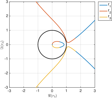
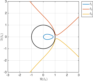
Branch change of roots $r_{k}$	Continuous roots $\ell_{k}$

Figure 1: Discontinuous and continuous roots $r_{k}$ and $\ell_{k}$

Theorem 3.1.

For any $\Delta x>0$, $\Delta t>0$ and $|z|>1$, the continuous roots of the cubic algebraic equation (3.8) are well separated according to

$$|\ell_{1}(z)|<1,\qquad|\ell_{2}(z)|>1,\qquad|\ell_{3}(z)|>1,\qquad\text{for all }z,$$ (3.10)

which defines the discrete separation property.

The proof of the theorem 3.1 is given in Appendix B.

Like in the continuous case (2.13), using the decay condition we obtain,

• for the left exterior domain $c_{1}(z)=0$, $j\leq 1$ and thus $\widehat{u}_{j}(z)=c_{2}(z)\,\ell_{2}^{j}(z)+c_{3}(z)\,\ell_{3}^{j}(z)$, $j\leq 1$

• for the right exterior domain $c_{2}(z)=c_{3}(z)=0$, $j\geq J-2$ and thus $\widehat{u}_{j}(z)=c_{1}(z)\,\ell_{1}^{j}(z)$, $j\geq J-2$

Let us now derive the boundary conditions for (R-CN) scheme.

Left boundary. On the left boundary we only need one relation. It is easy to see that

$$\widehat{u}_{j+1}(z)-\bigl{(}\ell_{2}(z)+\ell_{3}(z)\bigr{)}\,\widehat{u}_{j}(z)+\ell_{2}(z)\ell_{3}(z)\,\widehat{u}_{j-1}(z)=0.$$ (3.11)

Applying it for $j=1$ and denoting by $\mathcal{Z}^{-1}\{f(z)\}$ the inverse $\mathcal{Z}$-transform of $f(z)$, we obtain

$$\mathcal{Z}^{-1}\{\ell_{2}(z)\ell_{3}(z))\}*_{d}u_{0}^{(n)}-\mathcal{Z}^{-1}\{\ell_{2}(z)+\ell_{3}(z))\}*_{d}u_{1}^{(n)}+u_{2}^{(n)}=0,\quad n=0,1,2\dots,$$ (3.12)

where $*_{d}$ stands for the discrete convolution with respect to the temporal index $n$:

$$P*_{d}u_{i}^{(n)}=\sum_{k=0}^{n}P^{(k)}u_{i}^{(n-k)},$$

for $P=(P^{k})$ a sequence and $i$ an integer. Let us denote the convolution kernels by $k_{1,R}(z)=\ell_{2}(z)+\ell_{3}(z)$ and $k_{2,R}(z)=\ell_{2}(z)\ell_{3}(z)$ and by $Y_{i,R}$ the sequences of the inverse $\mathcal{Z}$-transform of kernel $k_{i,R}$ i.e. $Y_{i,R}=\mathcal{Z}^{-1}\{k_{i,R}(z)\}$. Then (3.12) can be written

$$Y_{2,R}*_{d}u_{0}^{(n)}-Y_{1,R}*_{d}u_{1}^{(n)}+u_{2}^{(n)}=0,\quad n=0,1,2\dots.$$ (3.13)

Right boundary. On the right boundary we need two relations since the fully discrete scheme involved four grid points. It is easy to see that

$$\widehat{u}_{j+2}(z)=\ell_{1}(z)^{2}\,\widehat{u}_{j}(z),\qquad\text{and}\qquad\widehat{u}_{j+1}(z)=\ell_{1}(z)\,\widehat{u}_{j}(z),$$ (3.14)

Applying them for $j=J-2$ and using inverse $\mathcal{Z}$-transformation, we obtain

$$u_{J}^{(n)}-Y_{4,R}*_{d}u_{J-2}^{(n)}=0,\quad u_{J-1}^{(n)}-Y_{3,R}*_{d}u_{J-2}^{(n)}=0,\quad n=0,1,2\dots,$$ (3.15)

where $k_{3,R}(z)=\ell_{1}(z)$ and $k_{4,R}(z)=\ell_{1}^{2}(z)$.

Remark 3.1.

We can easily obtain continuous roots $\ell_{k}$. We compute roots $r_{k}(z)$ where $z=\rho e^{i\theta}$ for a fixed radius $\rho$ and various angle $\theta$ thanks to (3.9). For each values of $\theta$, we sort roots thanks to the relation $r_{1}(\theta)<r_{2}(\theta)<r_{3}(\theta)$.

Remark 3.2.

We draw on Figure 2 (top figures) the behaviour of the inverse $\mathcal{Z}$-transform only for the two kernels $k_{1,R}(z)$ and $k_{3,R}(z)$ (the behavior of $k_{2,R}(z)$ and $k_{4,R}(z)$ being analogous). We clearly see that the signs of the coefficients alternate. This will possibly create subtractive cancellation errors when we will use them in the boundary convolutions. Following [4, 5], we modify the convolution kernels. The idea is to multiply a $\mathcal{Z}$-transformed kernel $k_{i,R}(z)$ by $\xi(z)=1+z^{-1}$ which corresponds to add two neighboured values in the series $\mathcal{Z}^{-1}\{k_{i,R}(z)\}$. We draw on Figure 2 (bottom figures) the behavior of the inverse $\mathcal{Z}$-transform for $\xi(z)k_{1,R}(z)$ and $\xi(z)k_{3,R}(z)$. We can clearly see that the signs of the coefficients do not alternate anymore. In the sequel we introduce the notations $Y_{i,R}^{\xi}=\mathcal{Z}^{-1}\{\xi(z)k_{i,R}(z)\}$. We refer to section 5 for more details on the numerical procedure used to compute the inverse $\mathcal{Z}$-transform for a kernel.

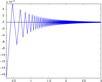
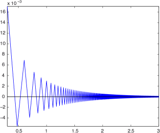
$\mathcal{Z}^{-1}(k_{1,R}(z))$	$\mathcal{Z}^{-1}(k_{3,R}(z))$
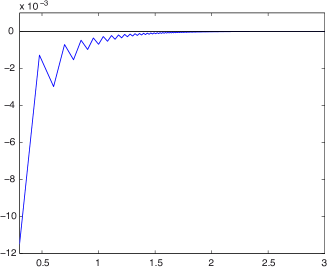
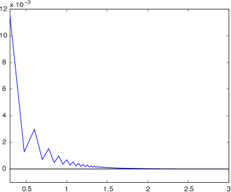
$\mathcal{Z}^{-1}(\xi(z)k_{1,R}(z))$	$\mathcal{Z}^{-1}(\xi(z)k_{3,R}(z))$

Figure 2: Coefficients of the inverse $\mathcal{Z}$-transform for the kernels $k_{i,R}(z)$, $i=1,3$ and kernels $\xi(z)k_{i,R}(z)$, $i=1,3$ with $\Delta t=4/2560$, $\Delta x=12/5000$ and $r=1.001$.

Remark 3.2 yields the algorithm used in Section 5 to solve numerically the problem. Assuming that the solution on the previous time level $(u_{j}^{(n)})_{0\leq j\leq J}$ is known, $(u_{j}^{(n+1)})_{0\leq j\leq J}$ is given for $n\geq 0$ by

$$\begin{cases}Y_{2,R}^{\xi}*_{d}u_{0}^{(n+1)}-Y_{1,R}^{\xi}*_{d}u_{1}^{(n+1)}+u_{2}^{(n+1)}=-u_{2}^{n},\\[5.69054pt] -\alpha u_{j-1}^{(n+1)}+(3\alpha+1)u_{j}^{(n+1)}-3\alpha u_{j+1}^{(n+1)}+\alpha u_{j+2}^{n+1}\\[5.69054pt] \hskip 56.9055pt=\alpha u_{j-1}^{(n)}-(3\alpha-1)u_{j}^{(n)}+3\alpha u_{j+1}^{(n)}-\alpha u_{j+2}^{(n)},\qquad 1\leq j\leq J-2,\\[5.69054pt] u_{J-1}^{(n+1)}-Y_{3,R}^{\xi}*_{d}u_{J-2}^{(n+1)}=-u_{J-1}^{n},\\[5.69054pt] u_{J}^{(n+1)}-Y_{4,R}^{\xi}*_{d}u_{J-2}^{(n+1)}=-u_{J}^{n},\end{cases}$$ (3.16)

with the mesh ratio $\alpha=U_{2}\Delta t/(2({\Delta x})^{3})$.

3.2 Discrete artificial boundary conditions for (C-CN) scheme

We treat here the case of the (C-CN) scheme for the interior nodes with a spatial index $j$ such that $2\leq j\leq J-2$. Since we consider a difference scheme with a five points stencil, we need two artificial boundary conditions on each side of the computational interval $[a,b]$.

In order to derive suitable artificial boundary conditions for the (C-CN) scheme (3.4) we follow the same procedure as in Section 3.1 for (R-CN) scheme. First we apply the $\mathcal{Z}$-transform with respect to the time index $n$, denoting by $\widehat{u}_{j}$ the $\mathcal{Z}$-transform of the sequence $(u_{j}^{(n)})_{n\in{\mathbb{N}}_{0}}$ we obtain from (3.4) the homogeneous fourth order difference equation:

$$\widehat{u}_{j+2}-\left(2-\frac{U_{1}(\Delta x)^{2}}{U_{2}}\right)\widehat{u}_{j+1}+\frac{4(\Delta x)^{3}}{U_{2}\Delta t}\frac{z-1}{z+1}\widehat{u}_{j}+\left(2-\frac{U_{1}(\Delta x)^{2}}{U_{2}}\right)\widehat{u}_{j-1}-\widehat{u}_{j-2}=0,$$ (3.17)

for the spatial index range $2\leq j\leq J-2$.

The solutions of this difference equation are again of the power form $\widehat{u}_{j}(z)=\sum_{k}c_{k}(z)\,\ell^{j}_{k}(z)$, where $\ell=\ell(z)$ solves now the quartic equation

$$\ell^{4}-\left(2-a\right)\ell^{3}+2p\ell^{2}+\left(2-a\right)\ell-1=0,$$ (3.18)

with $a=U_{1}(\Delta x)^{2}/U_{2}$ and $p=2\lambda(z-1)/(z+1)$.

Equation (3.18) admits four roots which can be computed numerically or analytically by the well-known Ferrari’s solution formula. As in the case of the cubic equation we identify these roots by continuity and refer to them as $\ell_{k}$ for $k=1,2,3,4$. Thus the general solution of (3.17) is of the form

$$\widehat{u}_{j}(z)=c_{1}(z)\,\ell_{1}^{j}(z)+c_{2}(z)\,\ell_{2}^{j}(z)+c_{3}(z)\,\ell_{3}^{j}(z)+c_{4}(z)\,\ell_{4}^{j}(z).$$

Like in the previous sections we can show the following theorem

Theorem 3.2.

For any $U_{1}\in{\mathbb{R}}$, $U_{2}>0$, $\Delta x>0$, $\Delta t>0$ and $|z|>1$, the continuous roots of the quartic algebraic equation (3.18) are well separated according to

$$|\ell_{1}(z)|<1,\qquad|\ell_{2}(z)|<1,\qquad|\ell_{3}(z)|>1,\qquad|\ell_{4}(z)|>1,\qquad\text{for all }z,$$ (3.19)

which defines the discrete separation property.

The proof of the theorem is given in Appendix C.

As previously, using theorem 3.2 and the decay condition of the solution we obtain

• for the left exterior domain $c_{1}(z)=c_{2}(z)=0$, $j\leq 2$ and thus $\widehat{u}_{j}(z)=c_{3}(z)\,\ell_{3}^{j}(z)+c_{4}(z)\,\ell_{4}^{j}(z)$, $j\leq 2$

• for the right exterior domain $c_{3}(z)=c_{4}(z)=0$, $j\geq J-2$ and thus $\widehat{u}_{j}(z)=c_{1}(z)\,\ell_{1}^{j}(z)+c_{2}(z)\,\ell_{2}^{j}(z)$, $j\geq J-2$

Right boundary. On the right boundary we need two relations. It is easy to see that

$$\widehat{u}_{j+2}(z)-\bigl{(}\ell_{1}(z)+\ell_{2}(z)\bigr{)}\widehat{u}_{j+1}(z)+\ell_{1}(z)\ell_{2}(z)\widehat{u}_{j}(z)=0,$$ (3.20)

$$\widehat{u}_{j+2}(z)-2(\ell_{1}(z)+\ell_{2}(z))\widehat{u}_{j+1}(z)+(\ell_{1}(z)+\ell_{2}(z))^{2}\widehat{u}_{j}(z)-(\ell_{1}(z)\ell_{2}(z))^{2}\widehat{u}_{j-2}(z)=0,$$ (3.21)

which will give a link between $u_{J}^{(n)}$, $u_{J-1}^{(n)}$, $u_{J-2}^{(n)}$ and $u_{J-4}^{(n)}$ with $j=J-2$.

For brevity of the notation we introduce $Y_{i,C}=\mathcal{Z}^{-1}\{k_{i,C}(z)\},i=1,2,3,4$ with

$$k_{1,C}(z)=\ell_{1}(z)+\ell_{2}(z),\qquad k_{2,C}(z)=\bigl{(}\ell_{1}(z)+\ell_{2}(z)\bigr{)}^{2},$$

$$k_{3,C}(z)=\ell_{1}(z)\ell_{2}(z),\qquad k_{4,C}(z)=\bigl{(}\ell_{1}(z)\ell_{2}(z)\bigr{)}^{2},$$

and we obtain from (3.23)–(3.24)

$$\begin{split}u_{J}^{(n)}-Y_{1,C}*_{d}u_{J-1}^{(n)}+Y_{3,C}*_{d}u_{J-2}^{(n)}&=0,\\ u_{J}^{(n)}-2Y_{1,C}*_{d}u_{J-1}^{(n)}+Y_{2,C}*_{d}u_{J-2}^{(n)}-Y_{4,C}*_{d}u_{J-4}^{(n)}&=0.\end{split}$$ (3.22)

Left boundary. On the left boundary we need now two relations. We can easily verify

$$\widehat{u}_{j}(z)-\bigl{(}\ell_{3}(z)+\ell_{4}(z)\bigr{)}\,\widehat{u}_{j-1}(z)+\ell_{3}(z)\ell_{4}(z)\,\widehat{u}_{j-2}(z)=0,$$ (3.23)

$$\widehat{u}_{j+2}(z)-2(\ell_{3}(z)+\ell_{4}(z))\widehat{u}_{j+1}(z)+(\ell_{3}(z)+\ell_{4}(z))^{2}\widehat{u}_{j}(z)-(\ell_{3}(z)\ell_{4}(z))^{2}\widehat{u}_{j-2}(z)=0,$$ (3.24)

which give a link between $u_{0}^{(n)}$, $u_{1}^{(n)}$, $u_{2}^{(n)}$, $u_{3}^{(n)}$ and $u_{4}^{(n)}$ setting $j=2$. Indeed, denoting by $Y_{i,C}=\mathcal{Z}^{-1}\{k_{i,C}(z)\}$, $i=5,6,7,8$ with

$$k_{5,C}(z)=\ell_{3}(z)+\ell_{4}(z),\qquad k_{6,C}(z)=(\ell_{3}(z)+\ell_{4}(z))^{2},$$

$$k_{7,C}(z)=\ell_{3}(z)\ell_{4}(z),\qquad k_{8,C}(z)=(\ell_{3}(z)\ell_{4}(z))^{2},$$

we obtain from (3.23)-(3.24)

$$\begin{split}Y_{7,C}*_{d}u_{0}^{(n)}-Y_{5,C}*_{d}u_{1}^{(n)}+u_{2}^{(n)}&=0,\\ -Y_{8,C}*_{d}u_{0}^{(n)}+Y_{6,C}*_{d}u_{2}^{(n)}-2Y_{5,C}*_{d}u_{3}^{(n)}+u_{4}^{(n)}&=0.\end{split}$$ (3.25)

Following Remark 3.2, we finally obtain the algorithm used in Section 5 to solve numerically the problem. Assuming that the solution $(u_{j}^{(n)})_{0\leq j\leq J}$ on the previous time level is known, then $(u_{j}^{(n+1)})_{0\leq j\leq J}$ is given for $n\geq 0$ by

$$\begin{cases}Y_{7,C}^{\xi}*_{d}u_{0}^{(n)}-Y_{5,C}^{\xi}*_{d}u_{1}^{(n)}+u_{2}^{(n)}=-u_{2}^{(n-1)},\\[5.69054pt] -Y_{8,C}*_{d}u_{0}^{(n)}+Y_{6,C}*_{d}u_{2}^{(n)}-2Y_{5,C}*_{d}u_{3}^{(n)}+u_{4}^{(n)}=-u_{4}^{(n-1)},\\[5.69054pt] \displaystyle{-\frac{\alpha}{2}u_{j-2}^{(n+1)}+(\alpha-\beta)u_{j-1}^{(n+1)}+u_{j}^{(n+1)}+(-\alpha+\beta)u_{j+1}^{(n+1)}+\frac{\alpha}{2}u_{j+2}^{(n+1)}}\\[5.69054pt] \quad=\displaystyle{\frac{\alpha}{2}u_{j-2}^{(n)}+(-\alpha+\beta)u_{j-1}^{(n)}+u_{j}^{(n)}+(\alpha-\beta)u_{j+1}^{(n+1)}-\frac{\alpha}{2}u_{j+2}^{(n+1)}},\quad 1\leq j\leq J-2,\\[5.69054pt] u_{J}^{(n)}-Y_{1,C}^{\xi}*_{d}u_{J-1}^{(n)}+Y_{3,C}^{\xi}*_{d}u_{J-2}^{(n)}=-u_{J}^{(n-1)},\\[5.69054pt] u_{J}^{(n)}-2Y_{1,C}^{\xi}*_{d}u_{J-1}^{(n)}+Y_{2,C}^{\xi}*_{d}u_{J-2}^{(n)}-Y_{4,C}^{\xi}*_{d}u_{J-4}^{(n)}=-u_{J}^{(n-1)}.\end{cases}$$ (3.26)

with the mesh ratios $\alpha=U_{2}\Delta t/(2({\Delta x})^{3})$ and $\beta=U_{1}\Delta t/(4\Delta x)$.

Remark 3.3.

Concerning the implementation, it is usual to define the midpoint unknown $v_{j}^{(n+1/2)}=(u_{j}^{(n+1)}+u_{j}^{(n)})/2$, with $v_{j}^{(-1/2)}=u_{j}^{(0)}$. In this case, (3.16) for the (R-CN) scheme reads

$$\begin{cases}\displaystyle Y_{2,R}^{\xi,(0)}v_{0}^{(n+1/2)}-Y_{1,R}^{\xi,(0)}v_{1}^{(n+1/2)}+v_{2}^{(n+1/2)}=-v_{2}^{(n-1/2)}-\sum_{k=1}^{n}Y_{2,R}^{\xi,(k)}v_{0}^{(n+1/2-k)}-\\ \hskip 113.81102pt\displaystyle Y_{2,R}^{\xi,(n+1)}u_{0}^{(0)}/2+\sum_{k=1}^{n}Y_{1,R}^{\xi,(k)}v_{1}^{(n+1/2-k)}+Y_{1,R}^{\xi,(n+1)}u_{1}^{(0)}/2,\\[5.69054pt] v_{j}^{(n+1/2)}+\alpha\left(v_{j+2}^{(n+1/2)}-3v_{j+1}^{(n+1/2)}+3v_{j}^{(n+1/2)}-v_{j-1}^{(n+1/2)}\right)=u_{j}^{n},\ 1\leq j\leq J-2.\\[5.69054pt] \displaystyle-Y_{3,R}^{\xi,(0)}v_{J-2}^{(n+1/2)}+v_{J-1}^{(n+1/2)}=-v_{J-1}^{(n-1/2)}+\sum_{k=1}^{n}Y_{3,R}^{\xi,(k)}v_{J-2}^{(n+1/2-k)}+Y_{3,R}^{\xi,(n+1)}u_{J-2}^{(0)}/2,\\[5.69054pt] \displaystyle-Y_{4,R}^{\xi,(0)}v_{J-2}^{(n+1/2)}+v_{J}^{(n+1/2)}=-v_{J}^{(n-1/2)}+\sum_{k=1}^{n}Y_{4,R}^{\xi,(k)}v_{J-2}^{(n+1/2-k)}+Y_{4,R}^{\xi,(n+1)}u_{J-2}^{(0)}/2,\end{cases}$$ (3.27)

For the (C-CN) scheme, (3.26) reads for $\ 1\leq j\leq J-2$.

$$\begin{cases}\displaystyle Y_{7,C}^{\xi,(0)}v_{0}^{(n+1/2)}-Y_{5,C}^{\xi,(0)}v_{1}^{(n+1/2)}+v_{2}^{(n+1/2)}=-v_{2}^{(n-1/2)}-\sum_{k=1}^{n}Y_{7,C}^{\xi,(k)}v_{0}^{(n+1/2-k)}-\\ \hskip 113.81102pt\displaystyle Y_{7,C}^{\xi,(n+1)}u_{0}^{(0)}/2+\sum_{k=1}^{n}Y_{5,C}^{\xi,(k)}v_{1}^{(n+1/2-k)}+Y_{5,C}^{\xi,(n+1)}u_{1}^{(0)}/2,\\[5.69054pt] \displaystyle-Y_{8,C}^{\xi,(0)}v_{0}^{(n+1/2)}+Y_{6,C}^{\xi,(0)}v_{2}^{(n+1/2)}-2Y_{5,C}^{\xi,(0)}v_{3}^{(n+1/2)}+v_{4}^{(n+1/2)}\\ \displaystyle\quad=-v_{4}^{(n-1/2)}+\sum_{k=1}^{n}Y_{8,C}^{\xi,(k)}v_{0}^{(n+1/2-k)}+Y_{8,C}^{\xi,(n+1)}u_{0}^{(0)}/2-\sum_{k=1}^{n}Y_{6,C}^{\xi,(k)}v_{2}^{(n+1/2-k)}\\[5.69054pt] \displaystyle\qquad-Y_{6,C}^{\xi,(n+1)}u_{2}^{(0)}/2+2\sum_{k=1}^{n}Y_{5,C}^{\xi,(k)}v_{3}^{(n+1/2-k)}+Z_{5}^{(n+1)}u_{3}^{(0)},\\[5.69054pt] \displaystyle-\frac{\alpha}{2}v_{j-2}^{(n+1/2)}+(\alpha-\beta)v_{j-1}^{(n+1/2)}+v_{j}^{(n+1/2)}+(-\alpha+\beta)v_{j+1}^{(n+1/2)}+\frac{\alpha}{2}v_{j+2}^{(n+1/2)}=u_{j}^{n},\\[5.69054pt] \displaystyle Y_{3,C}^{\xi,(0)}v_{J-2}^{(n+1/2)}-Y_{1,C}^{\xi,(0)}v_{J-1}^{(n+1/2)}+v_{J}^{(n+1/2)}=-v_{J}^{(n-1/2)}-\sum_{k=1}^{n}Y_{3,C}^{\xi,(k)}v_{J-2}^{(n+1/2-k)}-\\ \hskip 113.81102pt\displaystyle Y_{3,C}^{\xi,(n+1)}u_{J-2}^{(0)}/2+\sum_{k=1}^{n}Y_{1,C}^{\xi,(k)}v_{J-1}^{(n+1/2-k)}+Y_{1,C}^{\xi,(n+1)}u_{J-1}^{(0)}/2,\\[5.69054pt] \displaystyle-Y_{4,C}^{\xi,(0)}v_{J-4}^{(n+1/2)}+Y_{2,C}^{\xi,(0)}v_{J-2}^{(n+1/2)}-2Y_{1,C}^{\xi,(0)}v_{J-1}^{(n+1/2)}+v_{J}^{(n+1/2)}\\ \displaystyle\quad=-v_{J}^{(n-1/2)}+\sum_{k=1}^{n}Y_{4,C}^{\xi,(k)}v_{J-4}^{(n+1/2-k)}+Y_{4,C}^{\xi,(n+1)}u_{J-4}^{(0)}/2-\sum_{k=1}^{n}Y_{2,C}^{\xi,(k)}v_{J-2}^{(n+1/2-k)}\\ \displaystyle\qquad-Y_{2,C}^{\xi,(n+1)}u_{J-2}^{(0)}/2+2\sum_{k=1}^{n}Y_{1,C}^{\xi,(k)}v_{J-1}^{(n+1/2-k)}+Y_{1,C}^{\xi,(n+1)}u_{J-1}^{(0)}.\end{cases}$$ (3.28)

Solving (3.27) or (3.28), we recover $u_{j}^{(n+1)}$ by $u_{j}^{(n+1)}=2v_{j}^{(n+1/2)}-u_{j}^{(n)}$.

4 The Sum-of-Exponentials Approach

An ad-hoc implementation of the discrete convolutions of the form

$$\sum_{k=1}^{n}X_{m}^{(k)}u_{j}^{(n-k)}$$

with convolution coefficients $X_{m}^{(n)}$ has still one disadvantage. The boundary conditions are non–local in time (and space for higher dimensions) and therefore computations are too expensive. As a remedy, to get rid of the time non-locality, we use as in [4] the sum of exponentials ansatz, i.e. to approximate the convolution coefficients $X_{m}^{(n)}$ by a finite sum (say $L_{m}$ terms) of exponentials that decay with respect to time. This approach allows for a fast (approximate) evaluation of the discrete convolution since the convolution can now be evaluated with a simple recurrence formula for $L_{m}$ auxiliary terms and the numerical effort per time step now stays constant.

4.1 The Exponential Approximation

To do so we will follow the ideas of [4] and approximate the coefficients of a sequence $X_{m}^{(n)}$ by the following sum-of-exponentials ansatz

$$X_{m}^{(n)}\approx\widetilde{X}_{m}^{(n)}:=\begin{cases}X_{m}^{(n)},&n=0,\dots,\nu_{m}-1,\\ \sum_{l=1}^{L_{m}}b_{m,l}q_{m,l}^{-n},&n=\nu_{m},\nu_{m}+1,\dots\,,\end{cases}$$ (4.1)

where $L_{m}\in{\mathbb{Z}}$, $\nu_{m}\geq 0$ are given integer parameters, e.g. $L_{m}=20$, $\nu_{m}=2$, that have to be chosen appropriately to guarantee good approximation properties of $\widetilde{X}_{m}^{(n)}$. In the following, $X_{m}^{(n)}$ has to be seen as $Y_{m,R}^{\xi,(n)}$ or $Y_{m,C}^{\xi,(n)}$ respectively for (R-CN) and (C-CN) schemes.

In [4] the authors presented a deterministic method of choosing such an optimal approximation, i.e. finding the set $\{b_{m,l},q_{m,l}\}$ for fixed $L_{m}$ and $\nu_{m}$.

The “split” definition of $\widetilde{X}_{m}^{(n)}$ in (4.1) is motivated by the fact that the implementation of the discrete TBCs involves a convolution sum with $k$ ranging only from 1 to $k=n$. Since the first coefficient $X_{m}^{(0)}$ does not appear in this convolution, it makes no sense to include it in our sum-of-exponential approximation, which aims at simplifying the evaluation of the convolution. Hence, one may choose $\nu_{m}=1$ in (4.1). We observe numerically that the two first coefficients have a larger magnitude compared to the other ones. This suggests even to exclude $Z_{m}^{(1)}$ from this approximation and to choose $\nu_{m}=2$ in (4.1). We use this choice in our numerical implementation.

Let us fix $L_{m}$ and consider the formal power series:

$$g_{m}(x):=s^{(\nu_{m})}+s^{(\nu_{m}+1)}x+s^{(\nu_{m}+2)}x^{2}+\dots,\quad|x|\leq 1.$$ (4.2)

If there exists the $[L_{m}-1|L_{m}]$ Padé approximation

$$\tilde{g}_{m}(x):=\frac{P_{L_{m}-1}(x)}{Q_{L_{m}}(x)}$$

of (4.2), then its Taylor series

$$\tilde{g}_{m}(x)=\widetilde{X}_{m}^{(\nu_{m})}+\widetilde{X}_{m}^{(\nu_{m}+1)}x+\widetilde{X}_{m}^{(\nu_{m}+2)}x^{2}+\dots$$

satisfies the conditions

$$\widetilde{X}_{m}^{(n)}=X_{m}^{(n)},\qquad n=\nu_{m},\nu_{m}+1,\dots,2L_{m}+\nu_{m}-1,$$ (4.3)

due to the definition of the Padé approximation rule.

Theorem 4.1 ([4]).

Let $Q_{L_{m}}(x)$ have $L_{m}$ simple roots $q_{m,l}$ with $|q_{m,l}|>1,\quad l=1,\dots,L_{m}$. Then

$$\widetilde{X}_{m}^{(n)}=\sum_{l=1}^{L_{m}}b_{m,l}^{\phantom{n}}q_{m,l}^{-n},\qquad n=\nu_{m},\nu_{m}+1,\dots\,,$$ (4.4)

where

$$b_{m,l}:=-\frac{P_{L_{m}-1}(q_{m,l})}{Q_{L_{m}}^{\prime}(q_{m,l})}\,q_{m,l}^{\phantom{i}}\neq 0,\qquad l=1,\dots,L_{m}.$$ (4.5)

Evidently, the approximation of the convolution coefficients $X_{m}^{(n)}$ by the representation (4.1) using a $[L_{m}-1|L_{m}]$ Padé approximant to (4.2) behaves as follows: the first $2L_{m}$ coefficients are reproduced exactly, see (4.3). However, the asymptotics of $X_{m}^{(n)}$ and $\widetilde{X}_{n}^{(n)}$ (as $n\to\infty$) differ strongly – algebraic versus exponential decay.

4.2 Fast Evaluation of the Discrete Convolution

Let us consider the approximation (4.1) with $\nu_{m}=2$ for the discrete convolution kernel appearing in the discrete TBCs. With these “exponential” coefficients the approximated convolution

$$\tilde{C}_{m,j}^{(n)}:=\sum_{k=2}^{n}\widetilde{X}_{m}^{(k)}u_{j}^{(n-k)},\qquad\widetilde{X}_{m}^{(n)}=\sum_{l=1}^{L_{m}}b_{m,l}^{\phantom{n}}q_{m,l}^{-n},\qquad|q_{l}|>1,$$ (4.6)

of the discrete function $u_{j}^{(n-k)}$, $k=1,2,\dots$ with the coefficients $\widetilde{X}_{m}^{(n)}$ can be calculated by recurrence formulas, and this will reduce the numerical effort significantly.

A straightforward calculation ([4]) yields (for $\nu_{m}=2$):

$$\tilde{C}_{m,j}^{(n)}(\{u_{j}^{(n)})_{n}\}=\sum_{l=1}^{L_{m}}\tilde{C}_{m,j,l}^{(n)},\qquad n\geq 2,$$ (4.7)

where

$$\tilde{C}_{m,j,l}^{(2)}\equiv 0,$$

$$\tilde{C}_{m,j,l}^{(n)}=q_{m,l}^{-1}\tilde{C}_{m,j,l}^{(n-1)}+b_{m,l}^{\phantom{n}}q_{m,l}^{-1}u_{j}^{(n-2)},$$ (4.8)

$n=2,3,\dots$, $l=1,\dots,L_{m}$.

In order to use this fast evaluation procedure in our implementation point of view, we must transform it before to use it for midpoint $v_{j}^{(n+1/2)}$ unknown. It is easy to see that the second relation of (4.8) can be transformed as

$$\tilde{C}_{m,j,l}^{(n)}\{(u_{j}^{(n)})_{n}\}=b_{m,l}\sum_{k=2}^{n-1}q_{m,l}^{-k}u_{j}^{(n-k)}.$$ (4.9)

For example, let us consider the last TBC of (3.16)

$$u_{J}^{(n+1)}-Y_{4,R}^{\xi}*_{d}u_{J-2}^{(n+1)}=-u_{J}^{n}.$$

We have to see $Y_{4,R}^{\xi}*_{d}u_{J-2}^{(n+1)}$ as

$$Y_{4,R}^{\xi,(0)}u_{J-2}^{(n+1)}+Y_{4,R}^{\xi,(1)}u_{J-2}^{(n)}+\tilde{C}_{4,J-2}^{(n+1)}\{(u_{J-2}^{(n+1)})_{n}\}.$$

In order to get an equation for $v_{J-2}^{(n+1/2)}$, we write the previous relation at discrete time level $n$ and average the equations. We therefore get

$$v_{J}^{(n+1/2)}-Y_{4,R}^{\xi,(0)}v_{J-2}^{(n+1/2)}-Y_{4,R}^{\xi,(1)}v_{J-2}^{(n-1/2)}\\ =-v_{J}^{(n-1/2)}+\frac{1}{2}\left(\tilde{C}_{4,J-2}^{(n+1)}\{(u_{J-2}^{(n+1)})_{n}\}+\tilde{C}_{4,J-2}^{(n)}\{(u_{J-2}^{(n)})_{n}\}\right).$$ (4.10)

Thanks to (4.7) and (4.9), we obtain

$$v_{J}^{(n+1/2)}-Y_{4,R}^{\xi,(0)}v_{J-2}^{(n+1/2)}-Y_{4,R}^{\xi,(1)}v_{J-2}^{(n-1/2)}\\ =-v_{J}^{(n-1/2)}+\tilde{C}_{4,J-2}^{(n)}\{(v_{J-2}^{(n+1/2)})_{n}\}+\sum_{l=1}^{L_{m}}b_{4,l}q_{4,l}^{-n}v_{0}^{(1/2)}.$$ (4.11)

These equation then replaces the last one of (3.27).

These computations can be easily transferred to other convolutions appearing in other TBCs.

5 Numerical Results

In this section we first present the numerical procedure used to compute the inverse $\mathcal{Z}$-transforms required for the discrete absorbing boundary conditions. Then we consider two different examples for which we give some numerical results. The first example can be considered for either (R-CN) or (C-CN) scheme since $U_{1}=0$, $U_{2}=1$. The second one can only be considered for the (C-CN) scheme since in this ones $U_{1}=U_{2}=1$.

5.1 Numerical procedure for the inverse $\mathcal{Z}$-transform

In this section, we recall for a self-contained presentation the numerical procedure presented in [29] to compute the inverse $\mathcal{Z}$-transform.

Let us recall that if we consider the sequence $(u_{n})_{n\in{\mathbb{N}}}$, then its $\mathcal{Z}$-transform reads

$$U(z)=\sum_{k=0}^{\infty}u_{k}z^{-k},\quad|z|>R.$$

Assuming we know $U(z)$, we can recover the value of the sequence $u_{n}$ thanks to the relation

$$u_{n}=\frac{1}{2i\pi}\oint_{S_{r}}U(z)z^{n-1}dz,\quad r>R,$$

where $S_{r}$ denotes any circle of radius $r>R$. Performing the change of variable $z=re^{i\varphi}$, we obtain

$$u_{n}=\frac{r^{n}}{2\pi}\int_{0}^{2\pi}U(re^{i\varphi})e^{in\varphi}\,d\varphi.$$

Discretizing the angular variable $\varphi$ with $N$ nodes, we obtain the approximation

$$u_{n}\approx\frac{r^{n}}{N}\sum_{k=0}^{N-1}U\left(re^{i\frac{2\pi}{N}k}\right)e^{i\frac{2\pi}{N}kn}.$$

Let us now consider the finite sequence $\displaystyle\big{(}f_{n}\big{)}_{n=0}^{N-1}$. Its discrete Fourier transform is given by

$$F_{k}=\mathscr{F}\{f_{n}\}(k)=\sum_{n=0}^{N-1}f_{n}\omega_{N}^{-nk}$$

and we recover the value of $f_{n}$ through

$$f_{n}=\mathscr{F}^{-1}\{F_{k}\}(n)=\frac{1}{N}\sum_{k=0}^{N-1}F_{k}\omega_{N}^{nk}$$

where $\omega_{N}=e^{i\frac{2\pi}{N}}$. Therefore, if we define $U_{k}=U(r\omega_{N}^{k})$, we have

$$u_{n}\approx\frac{r^{n}}{N}\sum_{k=0}^{N-1}U_{k}\omega_{N}^{k}=r^{n}\mathscr{F}^{-1}\{U_{k}\}(n),\quad 0\leq n<N.$$

Thus, in order to obtain approximation of $u_{n}$, we have to multiply the inverse discrete Fourier transform of $U(z)$ evaluated at nodes $z_{k}=re^{2i\pi k/N}$ by $r^{k}$. The inverse discrete Fourier transform if easily obtain thanks for inverse fast Fourier transform.

Note that the choice of the inversion radius $r$ is crucial to guarantee the good approximation of the inverse $\mathcal{Z}$-transform and then the convergence of the numerical scheme as presented in Figure 8. Note that in [29] the best choice of $r$ seems to be $1.02$ while in our case it seems to be $1.001$. For a concise discussion on the choice of $r$ we refer the reader to [29].

5.2 Numerical Example 1

Let us first consider the example from Zheng, Wen and Han [28] which is concerned with the following equation ($U_{1}=0,~{}U_{2}=1$):

$$u_{t}+u_{xxx} =0,\qquad x\in{\mathbb{R}},$$ (5.1)

$$u(0,x) =e^{-x^{2}},\qquad x\in{\mathbb{R}},$$ (5.2)

$$u \to 0,\qquad|x|\to\infty.$$ (5.3)

The fundamental solution of equation (5.1) is [28]

$$E(t,x)=\frac{1}{\sqrt[3]{3t}}\operatorname{Ai}\left(\frac{x}{\sqrt[3]{3t}}\right),$$

where $\operatorname{Ai}(\cdot)$ is the Airy function. The exact solution of (5.1)-(5.3) can be written in terms of $E(t,x)$ as

$$u_{\rm exact}(t,x)=E(t,x)*e^{-x^{2}},$$

where $*$ denotes the convolution product on the whole real axis.

We present in Figure 3 the exact solution and the approximate solution obtained with (R-CN) scheme for $\Delta t=4/2560$, $\Delta x=12/5000$ and $r=1.001$ at different times $t=1,2,3,4$. We see that the (R-CN) solution is a very good approximation of the exact solution all along the time. No unphysical reflections can be seen at the boundaries. The same can be obtained by using the (C-CN) scheme.

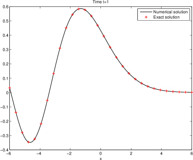
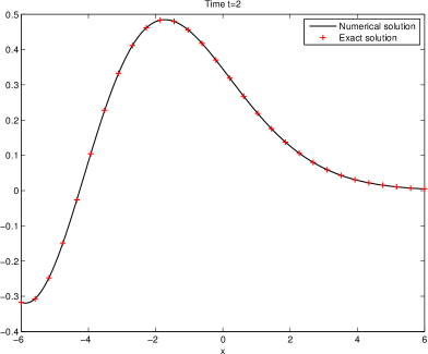
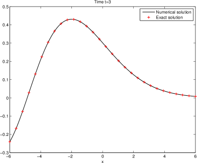
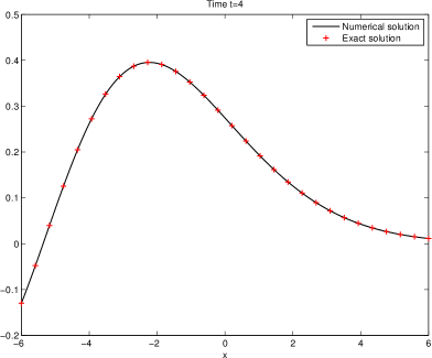
Figure 3: Numerical and exact solutions at times $t=1$, $t=2$, $t=3$ and final time $T=4$ for the first example with $\Delta t=4/2560$, $\Delta x=12/5000$ and $r=1.001$.

We present in Figure 4 a comparison at time $T=1$ between the exact solution and the approximate solution obtained with the sum of exponential approach either for various values of $N$ ($N=640,1280,2560$) and a fixed value of $L_{m}$ ($L_{m}=20$) or for a fixed value of $N$ ($N=2560$) and various values of $L_{m}$ ($L_{m}=10,20$). In each case $\Delta x=12/5000$ and $r=1.001$. We observe that the accuracy of the approximate solution depend on $N$ for a fixed $L_{m}$ and on $L_{m}$ for a fixed $N$.

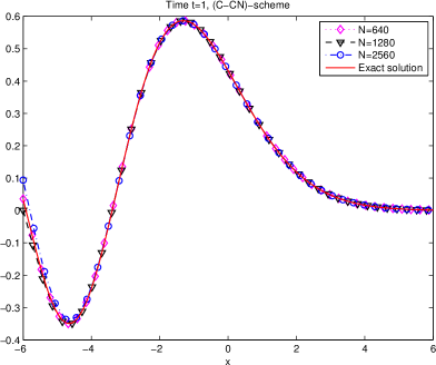
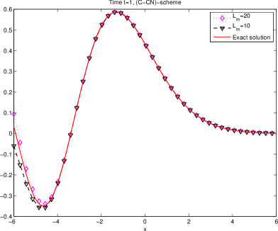
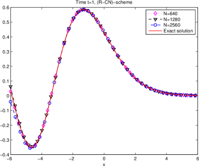
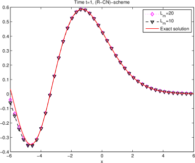
Figure 4: Comparison at time $T=1$ between the exact solution and the approximate solution obtained with the sum of exponential approach for the (C-CN) scheme (top figures) and the (R-CN)-scheme (bottom figures). The left figures are obtained with a fixed $L_{m}=20$ and various $N=640,1280,2560$ and the right figures with a fixed $N=2560$ and various $L_{m}=10,20$ for (C-CN) and (R-CN)-schemes.

Let us define as $e^{(n)}$ the relative $\ell^{2}$-error at time $t=n\Delta t$ given by:

$$e^{(n)}=\left\|u^{(n)}_{\rm exact}-u^{(n)}_{\rm num}\right\|_{2}/\left\|u^{(n)}_{\rm exact}\right\|_{2},$$

where we use trapezoidal rule to compute the $\ell^{2}$-norm. Note that here $u_{\rm num}$ stands for the numerical solution computed with either (R-CN) or (C-CN) scheme. We decided to compute from $e^{(n)}$ two error functions; first the maximum in time and secondly the $\ell^{2}$-error in time:

$$rel.ErrTm=\max_{0<n<N}\left(e^{(n)}\right),\qquad rel.ErrL2=\left(\Delta t\sum_{n=1}^{N}(e^{(n)})^{2}\right)^{1/2}.$$

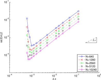
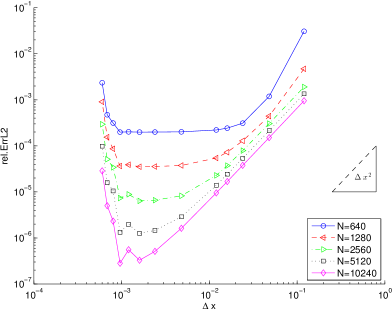
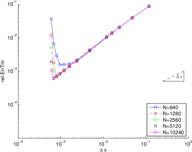
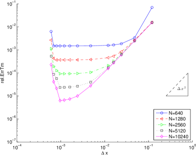
Figure 5: Relative errors with respect to $\Delta x$ at time $T=4$ for the (R-CN) scheme (figures on left) and the (C-CN)-scheme (figures on right) and for different values of $N$.

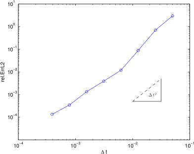
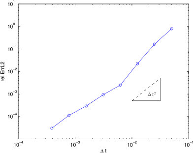
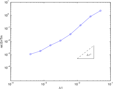
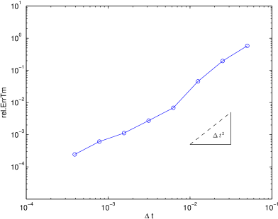
Figure 6: Relative errors with respect to $\Delta t$ at time $T=4$ for the (R-CN) scheme (figures on left) and the (C-CN)-scheme (figures on right) and for $J=20000$.

The behaviour of these two errors with respect to $\Delta x$ are presented in Figure 5. We observe that we obtained numerically the expected order of accuracy for each scheme: the (R-CN) scheme has a convergence order of one and the (C-CN) scheme is of order two. We can also see that for each value of $N$ there is a saturation phenomena for the error, for very small $\Delta x$ the round-off errors balances with the errors in the solution. Also, changing $\Delta x$ also modifies the roots of the cubic/quartic equations needed in the boundary convolution and the numerical inverse $\mathcal{Z}$-transform of the convolution kernels may degrade the overall accuracy (at least for the selected inversion radius).

We present in Figure 6 the $rel.ErrTm$ and $rel.ErrL2$ with respect to $\Delta t$ for $J=20000$ and $r=1.001$. Again we obtain for each scheme a numerical rate of convergence of order two in time. Surprisingly, the saturation effects from the previous figure do not show up, although with smaller $\Delta t$ the size of the boundary convolutions is increasing and this often leads to additional errors.

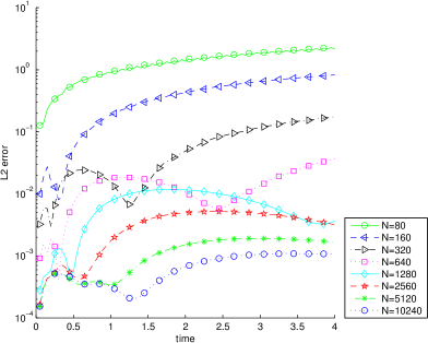
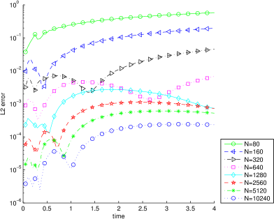
Figure 7: Evolution of the $\ell^{2}$ error between $T=0$ and $T=4$ for the (R-CN) scheme (figure on left) and the (C-CN)-scheme (figure on right) and for $J=20000$ and various values of $N$.

We present in Figure 7 the evolution of the $\ell^{2}$-error with respect to time for various values of $N$, $J=20000$ and $r=1.001$. As expected, the error decreases for increasing $N$, i.e. finer mesh size. In any case, the error remains moderately bounded over the whole simulation time which shows the usefulness of the proposed method. At the beginning the first increase is due to the interaction with the artificial boundaries and the second long term growth is due to an accumulation effect of errors, e.g. due to the increasing time convolution at the boundaries.

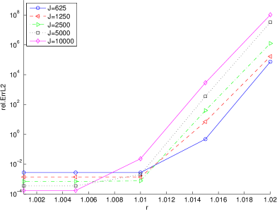
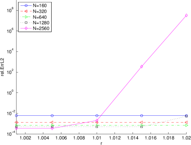
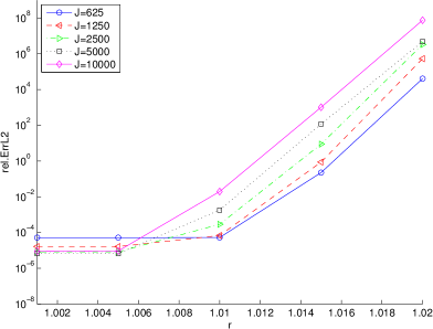
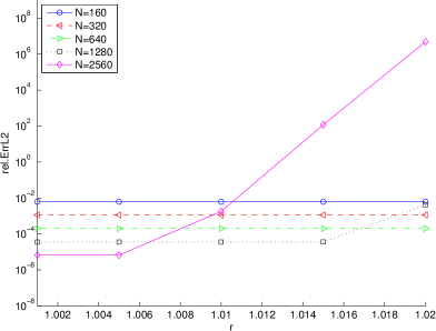
Figure 8: Error with respect to $r$ at time $T=4$ for the (R-CN) scheme (top figures) and the (C-CN)-scheme (bottom figures) with either $N=2560$ and various $J$ (figures on the left) or $J=5000$ and various $N$ (figures on the right).

We present in Figure 8 the $rel.ErrL2$ with respect to $r$ for each scheme and either with $N=2560$ and various $J$ or $J=5000$ and various $N$. The choice of $r$ in the inverse $\mathcal{Z}$-transform procedure is clearly impacting the error and depend on the values of $J$ and $N$. It seems that our choice, $r=1.001$, is a good choice for a large set of values of $N$ and $J$.

5.3 Numerical Example 2

Let us now consider a second example. We consider the dispersive equation (1.5) with $U_{1}=U_{2}=1$ and we choose as initial condition

$$u_{0}(x)=\exp(-8(x-5)^{2})\sin\left(\frac{50\pi}{4}\right),$$

for $0\leq x\leq 10$ and for a final time $T=4.8\times 10^{-4}$. This example was already considered in [6]. Note that using the Fourier transform, the problem being a linear and periodic problem, we can compute the exact solution ${u}_{\rm exact}(t,x)$. Indeed, applying the Fourier transformation in the space variable to the equation (1.5) we obtain

$$\widehat{u}_{t}+i\xi\widehat{u}-i\xi^{3}\widehat{u}=0,$$

where $\xi$ stands for the Fourier variable. Then it is easy to see that the transformed exact solution reads

$$\widehat{u}_{\rm exact}(t,\xi)=\widehat{u}_{0}\exp\left(-\left(i\xi-i\xi^{3}\right)t\right).$$

Using the inverse Fourier transform we have the exact solution of the problem. A reference solution is computed using 50000 points in space and 2560 iterations in time and used for Figures 9 and 10.

We present in Figure 9 the exact solution and the approximate solution obtained with (C-CN) scheme for $\Delta t=T/2560$, $\Delta x=10/5000$ and $r=1.001$ at final time. We see that the (C-CN) solution is a very good approximation of the exact oscillatory solution, the two solutions are nearly indistinguishable.

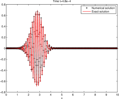
Figure 9: Numerical and exact solutions at final time for the second example with $\Delta t=T/2560$, $\Delta x=10/5000$ and $r=1.001$.

We present in Figure 10 the relative $\ell^{2}$-error $e^{(n)}$ computing at final time (i.e. for n=N) with respect to $\Delta x$ and for various values of $N$ and $r=1.001$. Again, we see that we obtain the order two as predicted. As for the first example there is a saturation phenomena.

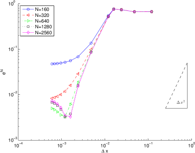
Figure 10: Relative error $e^{(N)}$ with respect to $\Delta x$ for various values of $N$ using (C-CN) scheme for the second example

Conclusion and Outlook

In this work we presented some new discrete absorbing boundary conditions adapted to two different numerical schemes for the linearized KdV equation (1.5). The orders of each scheme in time and space are shown numerically and given evidence that they are not perturbed by the discrete absorbing boundary conditions. To speed up the calculations of the costly boundary convolutions, especially in higher-dimensional cases, we proposed to use the sum-of-exponentials ansatz. We gave finally two numerical examples that supported our theoretical findings.

Future work will be to design an automatic good choice of the inversion radius, establish a transformation rule in the spirit of [4] for the KdV equation, treat the 2D and the nonlinear case.

Appendix A Proof of theorem 2.1

We saw in Remark 2.1 that the dispersive constant $U_{2}$ can be forced to be equal to $1$. Without loss of generality, we therefore consider for this proof $U_{2}=1$. The behavior of the roots is given on Figure 11.

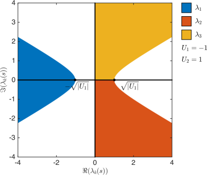
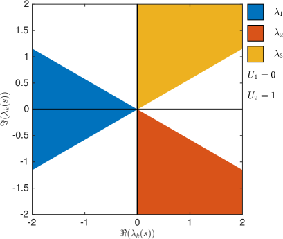
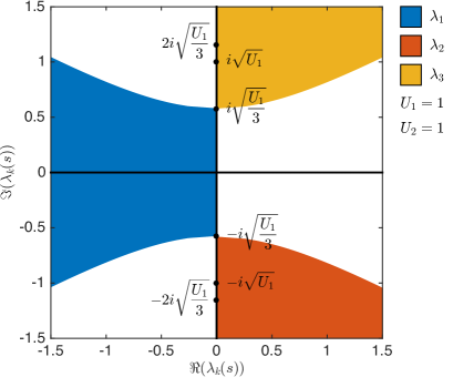
Figure 11: Roots $\lambda_{1}(s)$, $\lambda_{2}(s)$, $\lambda_{3}(s)$ to the equation (2.10) for $U_{1}=-1,\ 0,\ 1$ and $U_{2}=1$.

We prove here the result for stricly positive or negative velocity $U_{1}$. In both cases, we want to determine the domains $\mathbb{D}_{k}$, image of $\mathbb{C}^{+}=\{z\in\mathbb{C},\ \text{Re }z>0\}$, by roots $\lambda_{k}$ defined by (2.11)

$$\begin{array}[]{ccl}{\mathbb{C}}^{+}&\longrightarrow&\mathbb{D}_{k}\\ s&\longmapsto&\lambda_{k}(s).\end{array}$$

Since ${\mathbb{C}}^{+}$ is simply connected, we just have to identify the boundary of each domain $\mathbb{D}_{k}$ and a single point inside it to completely determined them. The boundaries are given by the image of $s=\varepsilon+i\xi$, $\varepsilon>0$, $\varepsilon\ll 1$ and $\xi\in{\mathbb{R}}$.

A.1 Case $U_{1}>0$

We perform an asymptotic expansion with respect to $\varepsilon$. Let us define $A=\sqrt{|\xi^{2}-(4/27)U_{1}^{3}|}$, $B=((\xi+A)/2)^{1/3}$, $C=B-U_{1}/(3B)$ and $D=B+U_{1}/(3B)$. Let us consider $\xi>0$.

For $\xi^{2}>4U_{1}^{3}/27$, the general expression for roots is for $k=1,2,3$

$$\lambda_{k}=-\left(\omega^{k-1}Be^{i\pi/6}-\frac{U_{1}}{3}\frac{1}{\omega^{k-1}Be^{i\pi/6}}\right)+\left(\omega^{k-1}Be^{2i\pi/3}-\frac{U_{1}}{3}\frac{1}{\omega^{k-1}Be^{2i\pi/3}}\right)\frac{\varepsilon}{3A}+O(\varepsilon^{2}),$$

and we have

$$\begin{array}[]{l}\displaystyle\lambda_{1}(s)=-\left(\frac{\sqrt{3}}{2}C+\frac{i}{2}D\right)-\left(\frac{1}{2}C-i\frac{\sqrt{3}}{2}D\right)\frac{\varepsilon}{3A}+O(\varepsilon^{2}),\\[5.69054pt] \displaystyle\lambda_{2}(s)=-\left(-\frac{\sqrt{3}}{2}C+\frac{i}{2}D\right)-\left(\frac{1}{2}C+i\frac{\sqrt{3}}{2}D\right)\frac{\varepsilon}{3A}+O(\varepsilon^{2}),\\[5.69054pt] \displaystyle\lambda_{3}(s)=iD+C\frac{\varepsilon}{3A}+O(\varepsilon^{2}).\end{array}$$

It is easy to show that $A$, $B$, $C$ and $D$ are positive for any $\xi^{2}>4U_{1}^{3}/27$. Clearly, we have $\operatorname{Re}{\lambda_{1}}<0$, $\operatorname{Re}{\lambda_{2}}>0$ and $\operatorname{Re}{\lambda_{3}}>0$. Concerning $\lambda_{1}$, since $-C/2<0$ and $D/2>0$, domain $\mathbb{D}_{1}$ is located on the left and above the complex curve $-(\sqrt{3}C+iD)/2$. The conclusion for $\lambda_{2}$ is similar and we conclude that domain $\mathbb{D}_{2}$ is located on the left and below the complex curve $(\sqrt{3}C-iD)/2$. The domain $\mathbb{D}_{3}$ is located on the right of the complex curve $iD$.

For $\xi^{2}<4U_{1}^{3}/27$, we define $E=((i\xi+A)/2)^{1/3}$ and have $|E|=\sqrt{U_{1}/3}$. We therefore can write $E=\sqrt{U_{1}/3}e^{i\theta(\xi)}$ with $0<\theta(\xi)<\pi/6$. We obtain

$$\lambda_{k}(s)=-2\sqrt{\frac{U_{1}}{3}}i\sin{\left(\theta+(k-1)\frac{2\pi}{3}\right)}-2\sqrt{\frac{U_{1}}{3}}\cos{\left(\theta+(k-1)\frac{2\pi}{3}\right)}\frac{\varepsilon}{3A}+O(\varepsilon^{2}).$$

We can conclude that $\lambda_{1}$ is located on the left of the complex curve $if(\theta)$, $-\sqrt{U_{1}/3}<f(\theta)<0$, $\lambda_{2}$ is on the right of the complex curve $ig(\theta)$, $-\sqrt{U_{1}}<g(\theta)<-\sqrt{U_{1}/3}$ and $\lambda_{3}$ is on the right of $ih(\theta)$, $\sqrt{U_{1}}<h(\theta)<2\sqrt{U_{1}/3}$.

The situation is completely symetric if we consider $\xi<0$. We therefore recover the figure 11 and we have shown the separation property

$$\operatorname{Re}(\lambda_{1}(s))<0,\qquad\operatorname{Re}(\lambda_{2}(s))>0,\qquad\operatorname{Re}(\lambda_{3}(s))>0.$$

A.2 Case $U_{1}<0$

Like in the previous case, we perform an asymptotic expansion and consider $\xi>0$. Let us define $\tilde{A}=\sqrt{\xi^{2}+4|U_{1}|^{3}/27}$, $\tilde{B}=((\xi+\tilde{A})/2)^{1/3}$, $\tilde{C}=\tilde{B}-U_{1}/(3\tilde{B})$ and $\tilde{D}=\tilde{B}+U_{1}/(3\tilde{B})$. For any $\xi\in{\mathbb{R}}$, we have $\tilde{A}>0$, $\tilde{B}>0$, $\tilde{C}>0$ and $\tilde{D}>0$. The general expression for roots is for $k=1,2,3$

$$\lambda_{k}=-\left(\omega^{k-1}\tilde{B}e^{i\pi/6}-\frac{U_{1}}{3}\frac{1}{\omega^{k-1}\tilde{B}e^{i\pi/6}}\right)+\left(\omega^{k-1}\tilde{B}e^{2i\pi/3}-\frac{U_{1}}{3}\frac{1}{\omega^{k-1}\tilde{B}e^{2i\pi/3}}\right)\frac{\varepsilon}{3A}+O(\varepsilon^{2}).$$

Thus, the asymptotics of $\lambda_{k}$ are given by

$$\begin{array}[]{l}\displaystyle\lambda_{1}(s)=-\left(\frac{\sqrt{3}}{2}\tilde{C}+\frac{i}{2}\tilde{D}\right)-\left(\frac{1}{2}\tilde{C}-i\frac{\sqrt{3}}{2}\tilde{D}\right)\frac{\varepsilon}{3A}+O(\varepsilon^{2}),\\[5.69054pt] \displaystyle\lambda_{2}(s)=-\left(-\frac{\sqrt{3}}{2}\tilde{C}+\frac{i}{2}\tilde{D}\right)-\left(\frac{1}{2}\tilde{C}+i\frac{\sqrt{3}}{2}\tilde{D}\right)\frac{\varepsilon}{3A}+O(\varepsilon^{2}),\\[5.69054pt] \displaystyle\lambda_{3}(s)=i\tilde{D}+\tilde{C}\frac{\varepsilon}{3A}+O(\varepsilon^{2}).\end{array}$$

Thanks to the signs of $\tilde{A}$, $\tilde{B}$, $\tilde{C}$ and $\tilde{D}$, the conclusions can be drawn by a simliar study to the $U_{1}>0$ case and we have $\operatorname{Re}(\lambda_{1}(s))<0$, $\operatorname{Re}(\lambda_{2}(s))>0$ and $\operatorname{Re}(\lambda_{3}(s))>0$.

Appendix B Proof of theorem 3.1

We consider here the continuous roots $\ell_{k}$ of (3.8) and ordered them thanks to the relation $|\ell_{1}(z)|\leq|\ell_{2}(z)|\leq|\ell_{3}(z)|$. We defined $p=\mu(z-1)/(z+1)$. If we note $z=x+iy$, $(x,y)\in{\mathbb{R}}^{2}$, then

$$p=\lambda\frac{(x^{2}+y^{2}-1)+2iy}{(x+1)^{2}+y^{2}}.$$

Since $|z|>1$, we have $x^{2}+y^{2}-1>0$ and

$$\operatorname{Re}{p}>0.$$

Thus, instead of studying $\ell_{k}$ as functions of $z$, we now consider them as functions of variable $p$ and try to identify the domains $\mathbb{D}_{k}$

$$\begin{array}[]{llcl}\ell_{k}:&{\mathbb{C}}^{+}&\longrightarrow&\mathbb{D}_{k}\\ &p&\longmapsto&\ell_{k}(p)\end{array}$$

Let us first show that $\ell_{k}$ can not belong to the unit circle. Let us assume that there exists $\theta\in[0,2\pi)$ such that $\ell_{2}=e^{i\theta}$. Since $\ell_{k}$ is a root of (3.8), then

$$e^{3i\theta}-3e^{2i\theta}+(3+p)e^{i\theta}-1=0.$$

It leads to $p=e^{i\theta}-3+e^{-i\theta}-e^{2i\theta}$. We therefore obtain

$$\operatorname{Re}{p}=-2(\cos\theta-1)^{2}\leq 0.$$

We have a contradiction since we had assume that $\operatorname{Re}{p}>0$. Thus, $\ell_{k}$ can not belong to the unit circle. Since we consider the continuous roots $\ell_{k}$ and ${\mathbb{C}}^{+}$ is simply connected, then $\mathbb{D}_{k}\in B(0,1)$ or $\mathbb{D}_{k}\in\bar{B}(0,1)$, the complementary of $B(0,1)$ in ${\mathbb{C}}$. In order to find if $\mathbb{D}_{k}$ lie inside or outside the unit circle, we just have to determine the domains for a single value of $p$.

Next, we know that if we consider a third order algebraic equation

$$x^{3}+bx^{2}+cx+d=0$$

then its roots satisfies

$$\begin{array}[]{l}x_{1}+x_{2}+x_{3}=-b\\ x_{1}x_{2}+x_{2}x_{3}+x_{3}x_{1}=c\\ x_{1}x_{2}x_{3}=-d.\end{array}$$

Therefore, $\ell_{1}$, $\ell_{2}$ and $\ell_{3}$ satisfy

$$\begin{array}[]{l}\ell_{1}\ell_{2}\ell_{3}=1\\ \ell_{1}+\ell_{2}+\ell_{3}=3\\ \ell_{1}\ell_{2}+\ell_{2}\ell_{3}+\ell_{3}\ell_{1}=3+p.\end{array}$$

The first relation implies $|\ell_{1}|\leq 1\leq|\ell_{3}|$. We therefore automatically have one root which lies inside the unit circle and one outside. It remains to understand the behavior of $\ell_{2}(p)$. In order to see the location of $\ell_{2}$ in the complex plane, we can therefore take any value of $p$ such that $\operatorname{Re}{p}>0$. If we take $p=3$, we have

$$|\ell_{1}|\approx 0.18,\quad|\ell_{2}|\approx 2.34,\quad|\ell_{3}|\approx 2.34.$$

Thus, $|\ell_{2}(p)|>1$ for any $p\in\mathbb{C}^{+}$ and we have shown

$$|\ell_{1}(p)|<1,\quad|\ell_{2}(p)|>1,\quad|\ell_{3}(p)|>1,\quad p\in{\mathbb{C}}^{+}.$$

Appendix C Proof of theorem 3.2

The proof is similar to the previous one. Let us consider a root $\ell_{k}$ and show that it can not be equal to $e^{i\theta}$. Let us assume that $\ell_{k}=e^{i\theta}$. Then

$$e^{4i\theta}-(2-a)e^{3i\theta}+pe^{2i\theta}+(2-a)e^{i\theta}-1=0.$$

Since $a\in{\mathbb{R}}$, this leads to

$$p=2i((2-a)\sin\theta-\sin 2\theta)\in i{\mathbb{R}}.$$

But, $\operatorname{Re}{p}>0$. This is a contradiction and $\ell_{k}\neq e^{i\theta}$.
We moreover have

$$\begin{array}[]{l}\ell_{1}+\ell_{2}+\ell_{3}+\ell_{4}=2-a,\\ \ell_{1}\ell_{2}+\ell_{1}\ell_{3}+\ell_{1}\ell_{4}+\ell_{2}\ell_{3}+\ell_{2}\ell_{4}+\ell_{3}\ell_{4}=p,\\ \ell_{1}\ell_{2}\ell_{3}+\ell_{1}\ell_{2}\ell_{4}+\ell_{2}\ell_{3}\ell_{4}+\ell_{1}\ell_{3}\ell_{4}=a-2,\\ \ell_{1}\ell_{2}\ell_{3}\ell_{4}=-1.\end{array}$$

If we sort the roots as $|\ell_{1}|\leq|\ell_{2}|\leq|\ell_{3}|\leq|\ell_{4}|$, the last equation leads to

$$|\ell_{1}(p)|<1\quad\text{and}\quad|\ell_{4}(p)|>1.$$

Computing $\ell_{2}$ and $\ell_{3}$ for $p=1$ for example prove that $|\ell_{2}(p)|<1$ and $|\ell_{3}(p)|>1$. We therefore have the discrete separation property of the roots.

References

- [1] M.J. Ablowitz, and P.A. Clarkson, Solitons, nonlinear evolution equations and inverse scattering, Cambridge University Press, New York (1991).
- [2] X. Antoine, A. Arnold, C. Besse, M. Ehrhardt, and A. Schädle, A review of transparent and artificial boundary conditions techniques for linear and nonlinear Schrödinger equations, Commun. Comput. Phys., 4 (2008), 729-796.
- [3] X. Antoine, C. Besse, and S. Descombes, Artificial boundary conditions for one-dimensional cubic nonlinear Schrödinger equations, SIAM J. Numer. Anal. 43 (2006), 2272-2293.
- [4] A. Arnold, M. Ehrhardt, and I. Sofronov, Discrete transparent boundary conditions for the Schrödinger equation: fast calculation, approximation, and stability, Commun. Math. Sci. 1 (2003), 501-556.
- [5] A. Arnold, M. Ehrhardt, M. Schulte, and I. Sofronov, Discrete transparent boundary conditions for the Schrödinger equation on circular domains, Commun. Math. Sci. 10 (2012), 889-916.
- [6] W.L. Briggs, and T. Sarie, Finite difference solutions of dispersive partial differential equations, Math. Comput. Simul. 25 (1983), 268-278.
- [7] J. Cruz, Ocean Wave Energy - Current Status and Future Prospects, Springer, 2008.
- [8] M. Ehrhardt, Discrete artificial boundary conditions, PhD, Technische Universität Berlin, 2001.
- [9] M. Ehrhardt, and A. Arnold, Discrete transparent boundary conditions for the Schrödinger equation, Riv. Math. Univ. Parma 6 (2001), 57-108.
- [10] M. Ehrhardt, Discrete Transparent Boundary Conditions for Schrödinger-type equations for non-compactly supported initial data, Appl. Numer. Math. 58 (2008), 660-673.
- [11] C. Eilbeck, (1998) http://www.ma.hw.ac.uk/~chris/scott_russell.html
- [12] C.S. Gardner, J.M. Greene, M.D. Kruskal, and R.M. Miura, Method for solving the Korteweg-de Vries equation, Phys. Lett. 19 (1967), 1095-1097.
- [13] H. Gleeson, P. Hammerton, D.T. Papageorgiou, and J.-M. Vanden-Broeck, A new application of the Korteweg-de Vries Benjamin-Ono equation in interfacial electrohydrodynamics, Phys. Fluids 19 (2007), 031703
- [14] D.J. Korteweg, and G. de Vries, On the Change of Form of Long Waves Advancing in a Rectangular Canal, and on a New Type of Long Stationary Waves, Philosophical Magazine 39 (1895), 422-443.
- [15] N.A. Kudryashov, and I.L. Chernyavskii, Nonlinear Waves in Fluid Flow through a Viscoelastic Tube, Fluid Dynamics 41 (2006), 49-62.
- [16] Q. Mengzhao, Difference schemes for the dispersive equation, Computing, 31 (1983), 261–267.
- [17] L.A. Ostrovsky, and Y.A. Stepanyants, Do internal solitons exist in the ocean?, Reviews of Geophysics, 27 (1989), 293-310.
- [18] J.S. Russell, Report of the committee on waves, Rep. Meet. Brit. Assoc. Adv. Sci. 7th Liverpool (1837) 417, London, John Murray.
- [19] S.W. Schoombie, A discrete multiple scales analysis of a discrete version of the Korteweg-de Vries equation, J. Comp. Phys. 101 (1992), 55-70.
- [20] J. Shen, A new dual-Petrov-Galerkin method for third and higher odd-order differential equations: application to the KdV equation, SIAM J. Numer. Anal. 41 (2003), 1595-1619.
- [21] H. Washimi, and T. Taniuti, Propagation of ion-acoustic solitary waves of small amplitude, Phys. Rev. Lett. 17 (1966), 966.
- [22] G.B. Whitham, Linear and nonlinear waves, Wiley, New York, 1974.
- [23] J.D. Wright, Corrections to the KdV Approximation for Water Waves, SIAM J. Math. Anal. 37 (2005), 1161-1206.
- [24] N.J. Zabusky, and M.D. Kruskal, Interactions of Solitons in a Collisionless Plasma and the Recurrence of Initial States, Phys. Rev. Lett. 15 (1965), 240-243.
- [25] N.J. Zabusky, Phenomena Associated with the Oscillations of a Nonlinear Model String, in Mathematical Models in Physical Sciences, S. Drobot (ed.) Prentice-Hall, Englewood Cliffs, New Jersey, 1963.
- [26] W. Zhang, H. Li, and X. Wu, Local absorbing boundary conditions for a linearized Korteweg-de Vries equation, Phys. Rev. E 89 (2014), 053305.
- [27] C. Zheng, Numerical simulation of a modified KdV equation on the whole real axis, Numer. Math. 105 (2006), 315-335.
- [28] C. Zheng, X. Wen, and H. Han, Numerical Solution to a Linearized KdV Equation on Unbounded Domain, Numer. Meth. Part. Diff. Eqs. 24 (2008), 383-399.
- [29] A. Zisowsky, Discrete transparent boundary conditions for systems of evolution equations, PhD, Technische Universität Berlin, 2003.