Finite Size Effects in the Nagel-Schreckenberg Traffic Model

Abstract

We examine the Nagel-Schreckenberg traffic model for a variety of maximum speeds. We show that the low density limit can be described as a dilute gas of vehicles with a repulsive core. At the transition to jamming, we observe finite-size effects in a variety of quantities describing the flow and the density correlations, but only if the maximum speed $V_{\text{max}}$ is larger than a certain value. A finite-size scaling analysis of several order parameters shows universal behavior, with scaling exponents that depend on $V_{\text{max}}$. The jamming transition at large $V_{\text{max}}$ can be viewed as the nucleation of jams in a background of freely flowing vehicles. For small $V_{\text{max}}$ no such clean separation into jammed and free vehicles is possible.

I Introduction

The flow of traffic represents a many-particle non-equilibrium problem with important practical consequences. Traffic flow shows well defined collective behavior where the free flow of traffic at low density changes abruptly with growing density to a denser phase with jams. The jams themselves show organized motions with start-stop waves as the cars creep forward. In addition to free flow and jam phases, there are also instances of synchronized flow at low velocity. Understanding the collective dynamical behavior and controlling the jams will give insight into effective traffic management. The flow of traffic also gives us an example of a non-equilibrium system with a phase transition, and it is interesting to inquire into the cause of the transition and whether long-range correlations appear near the transition.

Traffic behavior has been studied for decades, using a variety of approaches, including fluid dynamics models Lighthill and Whitham (1955), Boltzmann equations Prigogine and Herman (1971), and most recently, cellular automaton (CA) approaches Chowdhury (2000); Helbing (2001); Nagatani (2002). In CA models, the vehicles occupy discrete sites and have discrete velocities, hopping from site to site according to simple rules. Despite their simplicity, these CA models appear to capture much of the collective behavior observed in real traffic.

In 1992, Nagel and Schreckenberg (NS) Nagel and Schreckenberg (1992) introduced a relatively simple CA model for traffic flow. The road is represented as a set of $L$ equally spaced sites, each of which can be occupied by at most one of $N$ vehicles. Vehicles have discrete velocities $v_{n}$ from $0$ to a maximum velocity $V_{\text{max}}$. The hopping dynamics follow 4 simple rules, applied in the following sequence. First, each car with $v_{n}<V_{\text{max}}$ increases its velocity by one. The gap to the next car $g_{n}=r_{{n+1}}-r_{n}-1$ is computed, where $r_{n}$ is the position of the n-th car. If the car has a speed greater than $g_{n}$, it will brake to reduce its speed to $g_{n}$ to prevent a collision (gap rule). Variations in driver behavior are modeled by then lowering the speed $v_{n}\to v_{n}-1$ with a fixed probability $p$. Finally, the position is updated via $r_{n}\to r_{n}+v_{n}$.

The NS model mimics some, but by no means all, of the observed features of traffic flow. As the first of a series of increasingly detailed CA traffic models, it has been widely studied during the past twenty years to understand the nature of the phase transition from free flow to jams. Nagel and Schreckenberg Nagel and Schreckenberg (1992) showed that at low density $d=N/L$, a free flow state occurred where the cars all have a speed of $V_{\text{max}}$ or $V_{\text{max}}-1$, with a mean speed of $V_{\text{max}}-p$. At a certain density, the steady state changes to a phase with a nonzero fraction of the cars participate in a jam of slowly moving or stopped vehicles. Nagel and Paczuski Nagel and Paczuski (1995) showed in a variant of the NS model, where cars with $V=V_{\text{max}}$ maintain their velocity as a kind of cruise control, that the jam lifetime showed a power law distribution at the transition to the jam phase. Lubeck et al. Lübeck et al. (1998) studied the density distribution in the NS model and suggested that the free flow and jam phases coexist after the transition. Chowdhury et al. Chowdhury et al. (1997, 1998) examined the gap distribution and time-headway distribution (the time delay between two consecutive cars passing a site) and also concluded that there is a two phase coexistence after the transition. Roters et al. Roters et al. (1999) investigated the dynamical structure factor and concluded that a continuous phase transition occurs, but later work Chowdhury et al. (2000); Roters et al. (2000) suggested that the simulations were not long enough and that the critical behavior was actually a crossover phenomenon. Kerner et al. Kerner et al. (2002) observed evidence of two first order phase transitions, with an intermediate phase of synchronized flow between the free flow phase and the jam phase.

Many quantities have been used to study the transition to the jam phase. A number of them use the velocity distribution, such as the number of stopped cars ($V=0$) Vilar and Souza (1994), slowly moving cars ($V\leq V_{\text{max}}/2$) Jost and Nagel (2003) or cars not moving at the speed limit ($V<V_{\text{max}}$) Nagel and Paczuski (1995). Other authors have chosen the number of vehicles forced to brake Miedema et al. (2014) or the difference between the average velocity and the free flow velocity Souza and Vilar (2009). All of these resemble order parameters, being nearly to zero in the free flow phase and nonzero in the jam phase. Other quantities have been studied that not necessarily zero in the free phase, but show an abrupt change at the transition, such as the vehicle flux Nagel and Schreckenberg (1992) or the change in the vehicle’s kinetic energy per step Zhang et al. (2011); Zhang and Zhang (2014). A number of different traffic correlations have also been studied, including different characteristic velocities in the spatial dynamical structure factor Lübeck et al. (1998), different maxima in the velocity-position correlation Roters et al. (1999), the gap or time-headway distribution Chowdhury et al. (1998), the number of cars moving cooperatively de Wijn et al. (2012) and velocity correlations among the cars Lakouari et al. (2014).

Despite this effort, a comprehensive picture of the transition in the NS model is still incomplete, with different approaches producing differing conclusions about the nature of the transition or the presence of long range order. In this paper, we will examine how the value of $V_{\text{max}}$ affects the transition. We will show that, while the static structure factor shows long range behavior appearing at the transition for any $V_{\text{max}}$, we only see finite-size effects in the order parameter for $V_{\text{max}}\gtrsim 6$. This indicates that the nature of the long range behavior is different at high and low values of $V_{\text{max}}$. We use these finite-size effects to extract the scaling behavior at the transition for several order parameters. Our work indicates that the onset of the jam phase can be analyzed as a two phase coexistence of free flow and localized jams, as others have observed Lübeck et al. (1998); Chowdhury et al. (1998); Roters et al. (1999). We show that the presence or absence of long range correlations can be attributed to a qualitative change in the way jams nucleate at high and low values of $V_{\text{max}}$.

Despite the fact that the NS model misses some features observed in actual traffic flow Kerner (2013); Kerner et al. (2014), it remains a useful model to probe the nature of a nonequilibrium phase transition. It also provides a backdrop to understand the transitions observed in real traffic flow, which exhibits an intermediate synchronized flow phase Kerner et al. (2002, 2014) in some conditions.

In section II of this paper, we review the details of our simulation and the quantities we use in our analysis. Section III presents a quantitative analytic model of the behavior of the free flow phase as a repulsive-core gas. Section IV contains our analysis of the phase transition, long range correlations and finite-size effects. Section V discusses how the value of $V_{\text{max}}$ affects the fluctuations of jammed regions and how that affects the finite-size effects we see. Our conclusions are summarized in Section VI.

II Methodology

All the simulations in this paper are done for a single lane track with periodic boundary conditions. The track lengths varied from 5,000 to 100,000. We initially distributed the cars uniformly around the track. The system was then evolved for at least $10^{6}$ time steps to form a random steady state, a time step being one update of all $N$ vehicle positions and velocities. We then sampled the system every ten time steps for the next $10^{7}$ to $10^{8}$ time steps, the exact length depending on the system size.

Since this is a non-equilibrium problem, we were careful to look for non-ergodic effects and sensitivity to initial conditions. We used different random seeds to generate 5-10 different steady states for each choice of density and track length. We also did simulations using two different random number generators. We have seen no evidence that the choice of initial condition or random generator affected our results, although we have seen the need for long simulation times (much longer than typically used) to ensure that we are seeing the steady state behavior. If you use the ending configuration of a system at a higher density, and use its ending configuration (minus a few cars) as a starting configuration at lower density, you see the same results as starting from an initially uniform distribution of cars for the lower density. The values we show in this paper represent averages over simulation time, initial condition and random number generator.

To analyze this model, we chose to study density correlations using the static structure factor $S(q)$

$$S(q)=\langle|\rho(q)|^{2}\rangle\qquad\rho(q)=\sum_{r=1}^{L}e^{-iqr}n(r)\,,$$

and the pair correlation $G(r)$

$$G(r)=\frac{1}{L}\sum_{q}e^{iqr}\left(\frac{S(q)}{N}-1\right)=\left\langle\frac{1}{N}\sum_{l=1}^{L}n(l)n(l+r)\right\rangle,$$

where $n(r)=1$ if there is a car at site $r$ and zero otherwise. The angle brackets denote an average over configurations. The other function we examine is the nearest neighbor distribution $P(r)$

$$P(r)=\left\langle\frac{1}{N}\sum_{n=0}^{N-1}\delta(r_{{n+1}}-r_{n},r)\right\rangle\,,$$

where $r_{n}$ denotes the position of the n-th car and $\delta(,)$ denotes a Kronecker delta. $P(r)$ is simply the probability that the distance to the next car ahead is equal to $r$ .

III Free Flow Regime

In this model, the only interaction between the vehicles is the gap rule, which comes into play only when the distance to the next car is less than or equal to $V_{\text{max}}$. At low density $d=N/L$, when the vehicle spacing is typically much larger than $V_{\text{max}}$, naively applying the other dynamical rules produces a steady state with each vehicle having a speed of $V_{\text{max}}$ or $V_{\text{max}}-1$ with a mean speed of $V_{\text{max}}-p$. If the vehicles have this speed distribution, the vehicle spacing evolves as a random walk with a diffusion constant of $p(1-p)$. However, this produces a steady state where all spacings between cars are equally likely, including spacings of less than $V_{\text{max}}$.

Therefore, even in the dilute regime, the gap rule followed by the random slowdown, forces some cars to spend a small fraction of the time at a speed of $V_{\text{max}}-2$ because the gap to the vehicle ahead of it is $V_{\text{max}}-1$. This vehicle will, on the next time step, have a gap of $V_{\text{max}}-1$ or larger. Thus each car has a “repulsive core” that strongly favors at least $V_{\text{max}}-2$ empty sites ahead of it. In Fig. 1 we show a typical example.

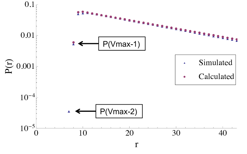
Figure 1: (Color online) Semilog plot of simulated $P(r)$ and that calculated from the Appendix for $V_{\text{max}}=9$ and $p=0.1$ at a density $d=0.04$, about half the critical density for the jams to form.

If we assume that no cars have a gap of less than $V_{\text{max}}-1$, we show in the Appendix that we can find $P(r)$ from a simple kinetic equation. For $r>V_{\text{max}}+2$, $P(r)$ obeys a drift-diffusion Fokker-Planck equation in the continuum limit

$$\frac{\partial P(r)}{\partial t}=\alpha\frac{\partial P(r)}{\partial r}+(p(1-p)+\alpha/2)\frac{\partial^{2}P(r)}{\partial r^{2}}\,,$$ (1)

where $\alpha=P(V_{\text{max}})$. The term $\alpha/2$ is the leading repulsive core correction to the diffusion constant. The steady state solution to the Eq. (1) for $r>V_{\text{max}}+2$ is

$$P(r)=P_{0}\exp\left(-\frac{\alpha}{p(1-p)+\alpha/2}\,r\right)\,,$$ (2)

where $P_{0}$ is a constant determined from solving the equations for $P(V_{\text{max}}+1)$ and $P(V_{\text{max}}+2)$, together with the normalization condition $\sum_{r}P(r)=1$.

There is a simple interpretation of the form of Eq. (2). Each vehicle has an excluded region of size $\approx V_{\text{max}}$ ahead of it. If the typical vehicle spacing is $L/N=1/d$, the effective free space between vehicles is $1/d-V_{\text{max}}\approx p(1\!-\!p)/\alpha+1/2$. An example of the agreement between the simulations and this analytic model are shown in Fig. 1.

The model above assumes that no vehicles have a gap of less than $V_{\text{max}}-1$. The event that first results in a gap of $V_{\text{max}}-2$ requires a configuration of three cars, each separated by a gap of $V_{\text{max}}-1$, with the middle car then slowing down by the randomization rule while the last car does not. Thus we need three body interactions to see violations of this analytic model.

Since three-body interactions are neglected, we expect that the pair correlation function $G(r)$ in the dilute limit can be found from the nearest neighbor distribution $P(r)$ via an Ornstein-Zernicke relation

$$G(r)=P(r)+\sum_{i=1}^{r-1}P(i)\,G(r-i)\,.$$ (3)

Figure 2(a) shows the nearest neighbor correlation $P(r)$ and the $G(r)$ we get from the simulations in this regime. Since $P(r)$ is vanishingly small for $r<V_{\text{max}}$, Eq. (3) predicts that $P(r)$ and $G(r)$ are identical up to $r=2V_{\text{max}}$ which Fig. 2(a) shows. The $G(r)$ that we find from the Eq. (3) is indistinguishable from the simulations. Figure 2(b) shows the corresponding structure factor $S(q)$. The peaks in $S(q)$ at multiples of $q=2\pi/V_{\text{max}}$ are simply the result of the repulsive core seen in $G(r)$. We note for future reference that $S(q)$ shows no upturn at $q\to 0$, indicating there is no long range order in the dilute regime.

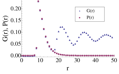
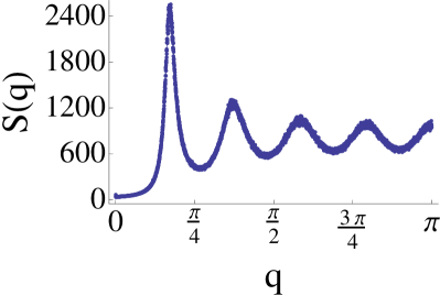
Figure 2: (Color online) (a) Simulated nearest neighbor distribution $P(r)$ and pair correlation $G(r)$ for $V_{\text{max}}=9$ and $p=0.1$ at a density $d=0.08$. (b) Structure factor $S(q)$ obtained from $G(r)$ through Eq. (3) and from simulations.

IV Finite Size Effects: Long-Range Correlation

As the vehicles density is raised, the repulsive core gas description we developed above remains qualitatively correct, with a gradual growth in the number of vehicles spaced at shorter distances $V_{\text{max}}-2$, $V_{\text{max}}-3$, …. When the jams appear, we see an abrupt change in the shape of the nearest neighbor distribution $P(r)$ with the sudden appearance of a nonzero fraction of vehicles with $r=1,2$. As Fig. 3(a) shows, the pair correlation $G(r)$ no longer agrees with $P(r)$ for $r\leq 2V_{\text{max}}$, and the Ornstein-Zernicke relation (3) between the two no longer holds. At the same time, Fig. 3(b) exhibits an upturn in $S(q)$ for $q\to 0$, indicating the appearance of long range correlations in the density.

We interpret this as indicating that the free flow phase is still stable, but that we have nucleated a new phase of localized jams that appear and disappear. Indeed, by examining the permanent stability of a localized jam, Gerwinski and Krug Gerwinski and Krug (1999) have shown that the jams should be stable at a density $\geq(1-p)/(1+V_{\text{max}}-2p)$, which is a higher density than where we see the onset of jams.

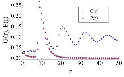
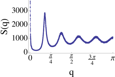
Figure 3: (Color online) (a) Nearest neighbor distribution $P(r)$ and pair correlation $G(r)$ for $V_{\text{max}}=9$ and $p=0.1$ for a density $d=0.088$, just above the density where jams appear. (b) Corresponding structure factor $S(q)$ with an upturn near $q\to 0$.

The upturn in $S(q)$ for small $q$ indicates some long-range order, which implies that we might observe finite-size effects in various quantities that are sensitive to the presence of that long range order. Figure 4 shows how the average velocity changes with density for different values of $V_{\text{max}}$ and different track lengths. For $V_{\text{max}}\lesssim 6$ we observe no length dependence. The figure also shows that once the density is well above the transition density, the system is insensitive to both the value of $V_{\text{max}}$ and the system size.

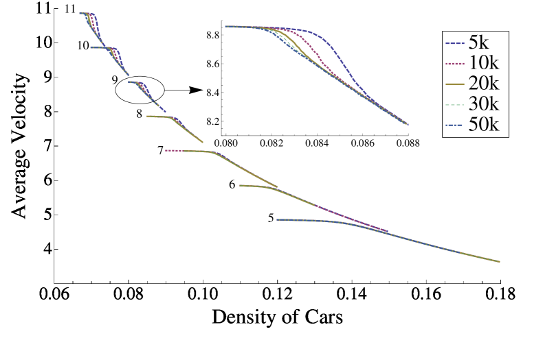
Figure 4: (Color online) The dependence of the mean velocity on density for various values of $V_{\text{max}}$ and $p=0.1$, and a variety of track lengths (shown as different colors).

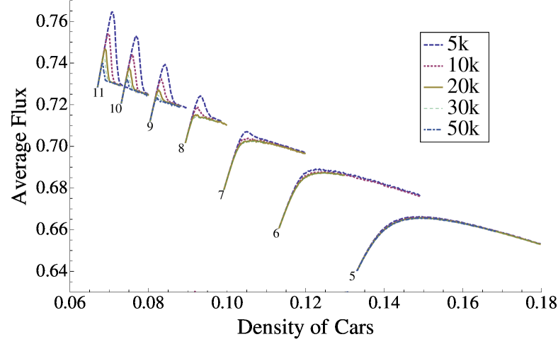
Figure 5: (Color online) The average flux versus density for various $V_{\text{max}}$ with $p=0.1$ and track lengths (different colors) of $L=$ 5k, 10k, 20k, 30k, 40k, 50k.

This size sensitivity is even more apparent in the mean flux of vehicles, presented in Fig. 5. As in the previous figure, it is only for $V_{\text{max}}\gtrsim 6$ that we see this size sensitivity. It also means that in a system of smaller size, the vehicle flux is actually higher than it is in larger systems, and that the size of the effect depends on $V_{\text{max}}$. This behavior is the reverse of what one would expect from hysteresis, where a large system would get trapped in a high flux free flow regime while a smaller system would not.

Since the value of $V_{\text{max}}$ represents the number of degrees of freedom for each car, it is not surprising that the finite-size behavior can depend on the number of degrees of freedom, as it does in equilibrium systems. However, we do not have any clear evidence that there is a critical value of $V_{\text{max}}$ for which the finite-size effects appear, but they are clearly suppressed for $V_{\text{max}}\leq 5$.

To characterize the transition, we need a quantity sensitive to the presence of jams. We discussed in the Introduction a variety of choices that others have used that are based on the velocity distribution. In this study, where we focus on the spatial distribution of the cars, we have used the gaps rather than the vehicle speeds to characterize the jams. The gap rule, however, produces a strong correlation between the speed of a vehicle and the distance to the next car, so our order parameter is closely related to these other choices.

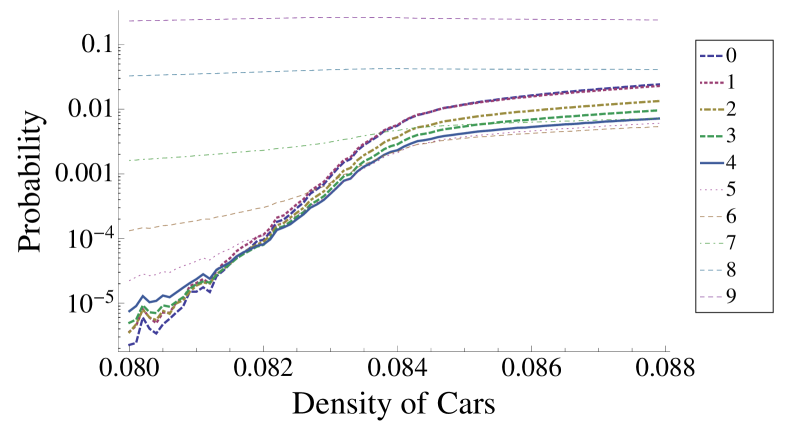
Figure 6: (Color online) Probability of finding a gap of a particular size for various densities for $V_{\text{max}}=9$ and $p=0.1$.

Figure 6 shows how the probability of finding gaps of different sizes varies with density near the transition. We see that the probability of having a gap $\leq V_{\text{max}}/2$ changes dramatically here. Therefore, we will define the order parameter $x_{0}$ to be the fraction of vehicles with a gap $\leq V_{\text{max}}/2$. We could have used just the vehicles with a gap of zero Vilar and Souza (1994), but using all of these gaps gives us more reliable statistics.

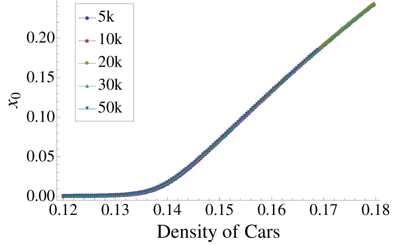
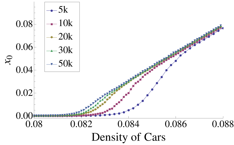
Figure 7: (Color online) Plots of the probability of having gap $\leq V_{\text{max}}/2$ for different track lengths and $p=0.1$ for (a) $V_{\text{max}}=5$ and (b) $V_{\text{max}}=9$.

Figure 7 shows that this order parameter $x_{0}$ exhibits the same finite-size effects, including its dependence on $V_{\text{max}}$, that we observed for the mean flux and velocity. These finite-size effects observed for $V_{\text{max}}\gtrsim 6$ are most pronounced for small systems, not large systems, unlike the hysteresis seen in an equilibrium first order transition.

In order to examine the long range correlations in this transition, we use a finite-size scaling approach Fisher (1967); Barber (1983); Ferrenberg and Landau (1991). Accordingly, we assume that the order parameter $x_{0}$ near the transition point depends on the size of the system as:

$$x_{0}=L^{-a_{0}}f(L/\xi)\,,$$ (4)

where $a_{0}$ is the scaling exponent, and $\xi$ is the correlation length, which itself depends on $L$ via

$$\xi\propto(d-d_{c}(L))^{-\nu}\,,$$ (5)

where $d_{c}(L)$ is the critical density.

In most finite-size scaling studies, the transition point itself is dependent on the system size. That effect is usually considered as a correction to scaling Ferrenberg and Landau (1991), and $d_{c}(L)$ then considered independent of $L$. We found that we got much better scaling fits by considering a length dependent critical density via

$$d_{c}(L)=d_{0}+cL^{-b}\,,$$ (6)

where $d_{0}$ is the critical density for the infinite system. We have tested Balouchi (2016) this approach on the 3d Ising model, which was studied by Ferrenberg and Landau Ferrenberg and Landau (1991) in their study of finite-size scaling corrections, and we find excellent agreement with their results.

To find the shift in the critical density, the typical approach Ferrenberg and Landau (1991) is to study a quantity like a susceptibility that has a peak at the transition. Our order parameter has no maximum at the transition, so we study its derivative Ferrenberg and Landau (1991) instead. While at first thought, a quantity like $\langle x_{0}^{2}\rangle$ might act like a susceptibility, we have found that this jamming transition is not like an equilibrium transition with large fluctuations in the order parameter correlations before the transition. Instead, we are seeing the nucleation of a different phase (the jams) in a background of the free phase, and the fluctuations in $x_{0}$ basically track $x_{0}$.

Instead, we examined the dynamic susceptibility, $\chi_{4}$, which was used to study glassy behavior in the NS model in the $p\to 1$ limit de Wijn et al. (2012)

$$\chi_{4}=\frac{1}{\langle{v^{2}}\rangle-\langle{v}\rangle^{2}}\,\left\langle\frac{1}{N}\sum_{i=1}^{N}\sum_{j=0}^{N}(v_{i}-\overline{v})(v_{j}-\overline{v})\right\rangle\,,$$ (7)

where $v_{i}$ is the velocity of the i-th car at a particular time and $\overline{v}$ denotes the mean speed of all the cars at that time. $\chi_{4}$ measures the number of vehicles that move cooperatively .

As Fig. 8 shows, $\chi_{4}$ has finite-size effects for $V_{\text{max}}\gtrsim 6$ with a peak as it goes through the transition. We assume $\chi_{4}$ obeys a finite-size scaling form

$$\chi_{4}=L^{-a_{4}}f(L/\xi)\,.$$

Using the peak in $\chi_{4}$ in Fig. 8 as the critical density, we find for $V_{\text{max}}=9$ and $p=0.1$ that the bulk transition occurs at $d_{0}=0.08122\pm 0.00004$, and the shift in the transition due to the finite system size has an amplitude of $c=0.375\pm 0.006$ and a scaling exponent of $b=0.54\pm 0.02$.

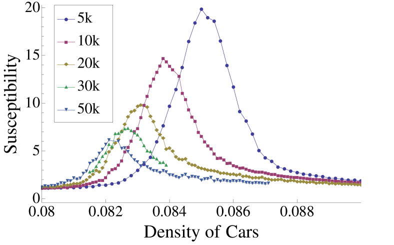
Figure 8: (Color online) The dynamic susceptibility $\chi_{4}$ for $V_{\text{max}}=9$, $p=0.1$ and various system sizes.

If we instead calculate the derivative of our order parameter $x_{0}$ and use its peak to calculate the shift of the transition point, we find $d_{0}=0.08267\pm 0.00001$, $c=9.415\pm 5.278$, and $b=0.956\pm 0.065$. There is no reason to expect that the peak in the derivative of $x_{0}$ should be at the same place as the $\chi_{4}$ peak, so it is not surprising the two results give different results for the shift in the transition point.

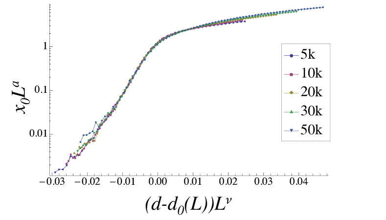
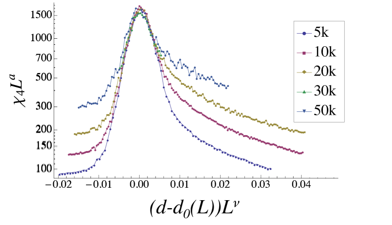
Figure 9: (Color online) Scaling plots of (a) $x_{0}L^{a_{0}}$ and (b) $\chi_{4}L^{a_{4}}$ versus $(d-d_{c}(L))L^{\nu}$ for $V_{\text{max}}=9$ and $p=0.1$.

After determining the shift in the transition, we collapse the data onto a single curve by plotting the quantity versus $(d-d_{c}(L))L^{\nu}$ and adjust the exponents to minimize the area bounded by the scaled data. The scaled plots of $x_{0}$ and $\chi_{4}$ are shown in Fig. 9. No matter which method we use to determine the shift in the transition point, we find that $x_{0}$ and $\chi_{4}$ produce values for the correlation length exponent $\nu$ of $0.13\pm 0.02$ and $0.14\pm 0.02$ respectively. The scaling exponent for the amplitude of $x_{0}$ is $a_{0}=0.24\pm 0.04$ and that of $\chi_{4}$ is $a_{4}=0.52\pm 0.02$. We also examined the scaling behavior of several alternative order parameters: the probability of a car having a speed $<V_{\text{max}}/2$ Jost and Nagel (2003), the difference between the mean speed and that of the free flow speed Souza and Vilar (2009), and the difference between the variance in the velocity and its value in the free flow regime Balouchi (2016). All of them gave results for $\nu$ and the scaling amplitude exponent $a_{0}$ that were consistent with those found for $x_{0}$.

We determined the values of $\nu$ and the scaling exponents for the amplitude of $x_{0}$ and $\chi_{4}$ for a range of values of $V_{\text{max}}$ and $p$. The values of the exponents for different values of $V_{\text{max}}$ and $p=0.1$ are shown in Fig. 10. The scaling behavior of $\chi_{4}$ and $x_{0}$ both yielded values for $\nu$ that were statistically the same for $V_{\text{max}}>7$. For $V_{\text{max}}=6$ and $V_{\text{max}}=7$, the finite-size dependence was so weak that we could not get reliable values for the scaling amplitude of $x_{0}$, and we were only able to extract a value for $\nu$ from $\chi_{4}$.

While this data does not imply a sharp change in the scaling behavior for $V_{\text{max}}=6$, it does indicate that the finite-size effects for $V_{\text{max}}>7$ are completely different than for $V_{\text{max}}\leq 6$, which is already apparent in Figs. 4 and 5. Figure 10 clearly shows that the exponent $\nu$ appears to vanish or take on unphysical negative values for $V_{\text{max}}=5$ and 6, indicating that the long range correlations are absent below $V_{\text{max}}=7$.

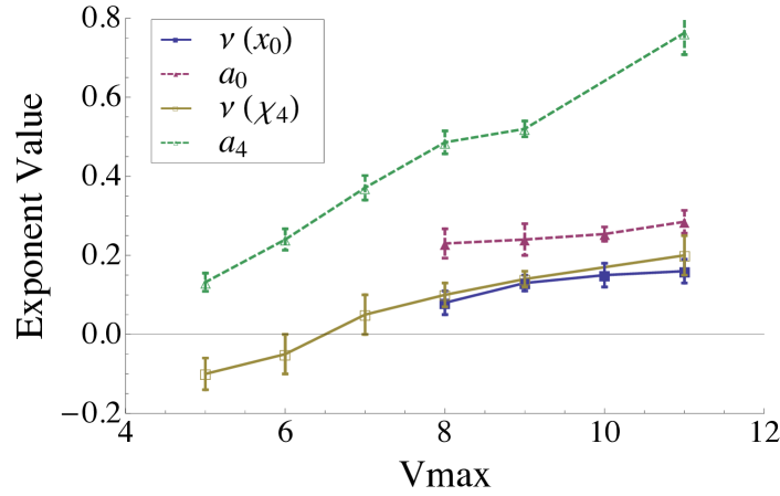
Figure 10: (Color online) Exponents $\nu$ and $a$ for various values of $V_{\text{max}}$, with $p=0.1$. The smaller error bars on $V_{\text{max}}=9$ result from using more track sizes.

Table 1 shows the scaling exponents for $V_{\text{max}}=9$ and three values of $p$, and we see no significant variation of $\nu$ or $a_{0}$ with $p$.

$p$	$\nu$	$a_{0}$
0.1	$0.13\pm 0.02$	$0.24\pm 0.04$
0.2	$0.12\pm 0.02$	$0.26\pm 0.04$
0.5	$0.14\pm 0.02$	$0.30\pm 0.01$

Table 1: (Color online) Exponents $\nu$ and $a_{0}$ for $V_{\text{max}}=9$ and various values of $p$.

The results agree with our expectation that we do not observe any variation of the exponents for $0<p<1$, since the value of $p$ controls the amount of stochastic behavior and the rate the system evolves through its configurations. Of course, in the special limits $p\to 0$ Zhang et al. (2011) and $p\to 1$ de Wijn et al. (2012) glassy, irreversible, behavior is observed instead.

V Growth of the Jams

As we noted earlier in Fig. 3, the finite-size effects that appear at the transition are accompanied by an upturn in the structure factor $S(q)$ for small $q$. It is therefore tempting to see whether the upturn in $S(q)$ merely reflects long range spatial correlations in $x_{0}$. We therefore define a local density $n_{0}(r)$ which is 1 if a vehicle is at site $r$ and the gap to the next car ahead is less than $V_{\text{max}}/2$. The extensive quantity $N_{0}=\sum_{r}n_{0}(r)\equiv x_{0}N$ provides a measure of the number of cars participating in a jam.

V.1 Spatial Correlations of Jams

To study the spatial correlations in $n_{0}(r)$, we examine the static structure factor

$$S_{0}(q)=\langle|\rho_{0}(q)|^{2}\rangle\qquad\rho_{0}(q)=\sum_{r}n_{0}(r)e^{-iqr}\,.$$

In Fig. 11 we show the magnitude of $S(q)$ and $S_{0}(q)$ at small values of $q$ for a several densities spanning the transition to jamming for $V_{\text{max}}=9$ and $p=0.1$. We see that most of the upturn in $S(q)$ for small $q$ in the transition to jamming comes from correlations in $n_{0}(r)$ of order less than a hundred lattice spacings or so. The behavior for $V_{\text{max}}=5$ is similar, except that the width of the peak in $S_{0}(q)$ (and $S(q)$) is much wider, indicating that the jammed regions are significantly smaller at low $V_{\text{max}}$.

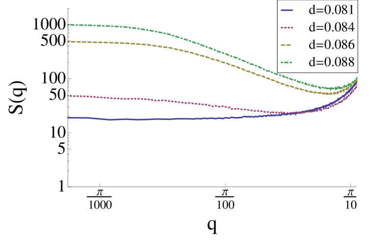
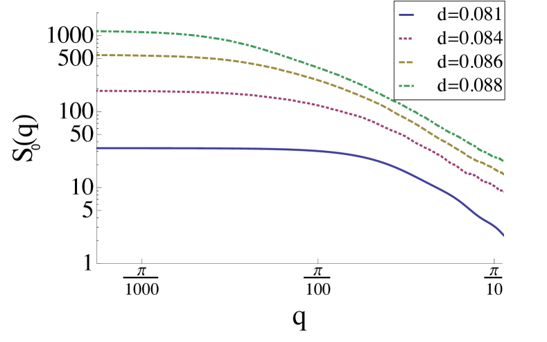
Figure 11: (Color online) Behavior of (a) the total structure factor $S(q)$ and (b) the structure factor for jammed vehicles $S_{0}(q)$ for small $q$. The data are for $V_{\text{max}}=9$, $p=0.1$ and $L=5000$. The densities correspond to before the transition, in the transition region, and beyond the transition.

This behavior is also visible in Fig. 12, where we display the variation of $S(q)$ and $S_{0}(q)$ with density for the longest wavelength $q=2\pi/L$ in our simulation.

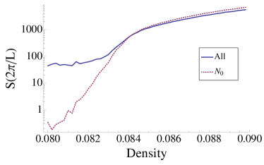
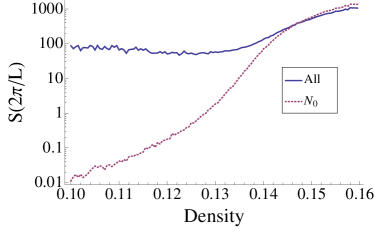
Figure 12: (Color online) Behavior of $S(q\!=\!2\pi/L)$ and $S_{0}(q\!=\!2\pi/L)$ for $L=10000$. (a) $V_{\text{max}}=9$ and (b) $V_{\text{max}}=5$, both with $p=0.1$.

The behavior for $V_{\text{max}}=5$, shown in Fig. 12(b) is very similar to that seen for $V_{\text{max}}=9$, so we can conclude that the upturn in $S(q)$ in the transition region is due to long-range correlations in $n_{0}(r)$. This is surprising, since we did not see finite-size effects for $V_{\text{max}}=5$. We will see in the next section that it is the dynamics and statistics of the jams that is different for the two situations.

V.2 Jam Dynamics

To explore the difference between the low $V_{\text{max}}$ and high $V_{\text{max}}$ behavior, we looked at the time evolution of system at the transition area. Figure 13 shows how $N_{0}(t)$ behaves for different densities for $V_{\text{max}}=9$ and $V_{\text{max}}=5$. The densities shown are chosen so that the system is initially in the pure free-flow phase, then early in the transition region near the peak flux from Fig 5, then late in the transition region, and finally in the jam phase. In the free flow phase, we see isolated fluctuations into the jam phase very rarely for $V_{\text{max}}\!=\!9$, while these fluctuations are more frequent in the $V_{\text{max}}\!=\!5$ simulations. In the transition region close to the peak in the flux shown in Fig. 5, the $V_{\text{max}}\!=\!9$ simulations still show isolated bursts of appearance of the jam phase, while for $V_{\text{max}}\!=\!5$ the number of jammed vehicles is fluctuating but always nonzero.

Figure 13: Time evolution of the number of cars in jam $N_{0}$ for a track of length 5,000 for $V_{\text{max}}=9$ (left) and $V_{\text{max}}=5$ (right) and $p=0.1$.

Since our order parameter $x_{0}$ for small $V_{\text{max}}$ might be showing this behavior due to an inability to cleanly separate freely flowing vehicles from jammed vehicles, we also used an order parameter that examines second neighbor correlations. Instead of just asking that the distance to the car ahead be less than $V_{\text{max}}/2$, we consider three cars in succession located at $r_{n}$, $r_{n+1}$, $r_{n+2}$ and require each pair of cars to be spaced by less than $V_{\text{max}}/2$.

$$\phi(r)=\begin{cases}1&r_{n}=r\mbox{ and }\\ &|r_{n+1}-r_{n}|<V_{\text{max}}/2\mbox{ and }\\ &|r_{n+2}-r_{n+1}|<V_{\text{max}}/2\\ 0&\mbox{otherwise\, ,}\\ \end{cases}$$

The total number of cars with this condition is $\Phi_{0}=\sum_{r}\phi_{(}r)$.

We show in Fig. 14 the fraction of the time the two order parameters are nonzero for $V_{\text{max}}=5$ and $V_{\text{max}}=9$. For $V_{\text{max}}=5$ both order parameters are always nonzero after $d=0.115$, but that is actually a density before the peak flux in Fig. 5 occurs for $V_{\text{max}}=5$, so the two order parameters become identical before the transition to jams occurs. For $V_{\text{max}}=9$, the two order parameters coincide and the transition from nearly zero to unity is the density range where we see finite-size effects.

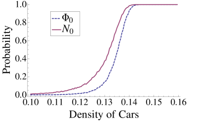
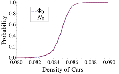
Figure 14: (Color online) Fraction of the time that the two order parameters $N_{0}$ and $\Phi_{0}$ are nonzero for different densities for (a) $V_{\text{max}}=5$ and (b) $V_{\text{max}}=9$.

So improving our definition of a jammed vehicle does not change the conclusion that the nucleation of the jams for $V_{\text{max}}\lesssim 6$ is qualitatively different than those for $V_{\text{max}}\gtrsim 7$.

The difference in behavior for different $V_{\text{max}}$ is also clearly visible in histograms of the fraction of the cars in a jam, $\Phi_{0}/N$. Figure 15 shows the histograms for the same simulations shown in Fig. 13. The peak at $\Phi_{0}/N=0$ is the vehicles in the free-flow phase. While the distributions for the free flow regime at low density and the jammed regime are similar for both values of $V_{\text{max}}$, they are clearly different in the transition regime. For $V_{\text{max}}\!=\!9$ the jam phase appears as a distinct phase in the transition region, while for $V_{\text{max}}\!=\!5$ this does not happen, with the distribution of jammed cars growing smoothly out of the free-flow phase.

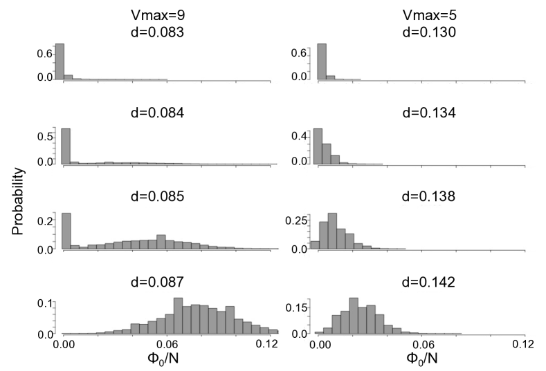
Figure 15: Histogram of $\Phi_{0}/N$ for the simulations show in Fig. 13.

Figure 16 shows how the length of the track affects themselves in the time evolution $\Phi_{0}$ and in the distribution of $\Phi_{0}$. The density in all of the plots is the same, but the histogram and the time evolution for the shortest track is characteristic of the free phase regime. For the intermediate track length, the behavior is that of two-phase coexistence. The longest track length data show it to be in the jam phase. Therefore we see that shorter track lengths inhibit the transition to jamming and thus we expect to see finite-size effects.

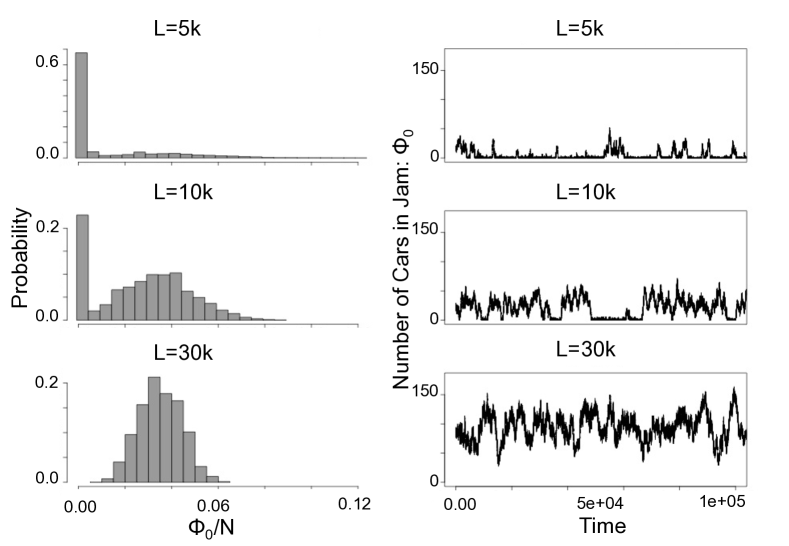
Figure 16: Time evolution and histogram of $\Phi_{0}/N$ for systems with same density $d=0.084$ and different lengths.

The transition region at high $V_{\text{max}}$ can thus be thought of as a coexistence of cars condensed into jams and cars flowing freely. The appearance of a single localized jam will reduce the density of freely flowing cars elsewhere, and this effect is more significant for shorter tracks. Since the probability of creating a jammed region drops as the density of freely flowing cars goes down, the appearance of one jam inhibits the appearance of an additional one, stabilizing the dilute gas of jams.

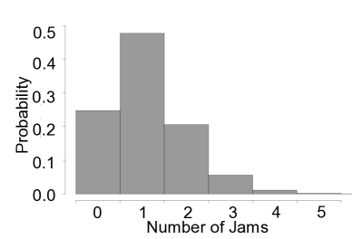
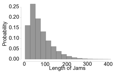
Figure 17: Statistics for 200,000 samples in a system of size $L=10,000$ for $V_{\text{max}}=9$, $p=0.1$ and $d=0.084$. (a) Distribution of number of jams (b) Distribution of jam lengths.

This picture favors a fewer large jams rather many small jams. Figure 17 shows a histogram of the number of jams for $V_{\text{max}}=9$ at a density $d=0.084$, and also the distribution of jam lengths. The distribution is not Poisson, as we would expect for independent events. Instead, we see a marked tendency for one or two large jams, with the probability of three or more jams greatly reduced. We find that the jam would be of order 50 sites in length, in agreement with the width of $S_{0}(q)$ for small $q$ seen in Fig. 11.

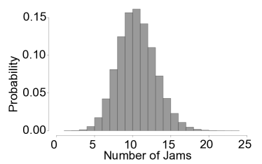
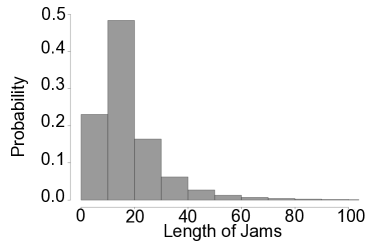
Figure 18: Statistics for 200,000 samples in a system of size $L=10,000$ for $V_{\text{max}}=5$, $p=0.1$ and $d=0.142$. (a) Distribution of number of jams and (b) Distribution of jam lengths.

For low $V_{\text{max}}$, the system does not break easily into tightly packed jams and a lower density of freely flowing cars. The nucleation of one jam does not depress the density of freely flowing cars sufficiently to inhibit the formation of subsequent jams. As a result, the low $V_{\text{max}}$ system does not have a clear transition region where isolated jams appear, and it is the isolated jams that are responsible for the finite-size effects we see at higher $V_{\text{max}}$. This is clearly seen in the distribution of numbers of jams and jam lengths shown in Fig. 18. The simulations were done at a density close to the peak flux for $V_{\text{max}}=5$. The jams are smaller and more frequent than in the $V_{\text{max}}=9$ data of Fig. 17.

Once the nucleation of one jam does not significantly inhibit the formation of a second one, we have reached the heavily jammed region and the finite-size effects that appear at high $V_{\text{max}}$ disappear. The mean velocity and flux then follow the relations shown in Figs. 4 and 5 that are insensitive to the value of $V_{\text{max}}$.

V.3 Coexistence at the Transition

This picture of a few localized jams condensing out of the free flow phase allows us to make a quantitative description of the finite-size effects in the large $V_{\text{max}}$ simulations. If we assume the jams consist of cars traveling as fast as the gap rule would allow, then their mean speed would be

$$V_{\text{J}}=\sum_{i<V_{\text{max}}/2}(i-1)\,P(i)\,,$$ (8)

and the fraction of the track occupied by the jams is

$$L_{\text{J}}=N\sum_{i<V_{\text{max}}/2}i\,P(i)\,.$$ (9)

Since $N_{0}$ is the number of cars in a jam, then the density of free cars is changed to

$$d_{\text{eff}}=\frac{N-N_{0}}{L-L_{\text{J}}}\,,$$ (10)

We then expect that the mean velocity of the mixture would be

$$V_{\text{tot}}=\frac{N_{0}}{N}V_{\text{J}}+\left(1-\frac{N_{0}}{N}\right)V_{\text{F}}(d_{\text{eff}})\,,$$ (11)

where $V_{\text{F}}(d_{\text{eff}})$ is the flow velocity in the free flow phase taken from the average velocity plot (Fig. 4) at an effective density $d_{\text{eff}}$ given by Eq. (10). We evaluate Eqs. (8), (9), and $V_{\text{F}}(d_{\text{eff}})$ directly from our simulations to find $V_{\text{tot}}$. Figure 19 shows the result of this for several track lengths. The agreement with the simulations is excellent in the transition region, and underestimates the mean velocity at higher density where this simple picture of two phase coexistence breaks down.

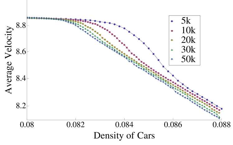
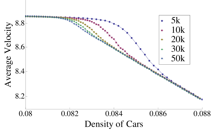
Figure 19: (Color online) (a) Calculated and (b) simulated average velocity for different track lengths versus density of cars for $V_{\text{max}}=9$ and $p=0.1$.

VI Conclusions

We have shown that the interactions in the NS model for a dilute gas of vehicles can be described as weakly interacting except for a repulsive interaction of range $\approx V_{\text{max}}$. The gap distribution can be found from solving the kinetic equations keeping only these pair interactions. Spatial correlations among cars further apart can be described quantitatively through an Ornstein-Zernicke relation.

As the density is raised to the point where jams form, we see that the nearest neighbor interactions fail to describe the density correlations. The jam formation results in a peak in the gap distribution $P(r)$ for small $r$ arising from jammed vehicles. At the same time, the structure factor $S(q)$ shows a significant upturn for small $q$, indicating the onset of long range correlations. These new correlations are not the result of including just second or third neighbor correlations.

Several authors Lübeck et al. (1998); Chowdhury et al. (1998); Roters et al. (1999) have noticed that the transition to jams can be described as the nucleation of isolated jams in a background of freely flowing cars. Our work shows that the characteristics of the transition depend on the value of $V_{\text{max}}$. In this regard, $V_{\text{max}}$ plays the role of the number of degrees of freedom (possible velocities) for each object, much like the role of the number of components of a spin variable in an equilibrium system.

Systems with $V_{\text{max}}\gtrsim 6$ show a transition with an intermediate phase that exhibits significant finite size effects. We attribute these effects to the existence of large isolated jams that coexist with the free flow phase in this intermediate regime. These large jams act to segregate vehicles and keep the free flow phase stable. The finite-size scaling analysis shows that these long range correlations appear to be universal, with scaling exponents that depend on $V_{\text{max}}$. We are able to quantitatively fit the overshoot seen in the vehicle flux in a finite size system by accounting for the segregation of the vehicles into jams. While our choice for an order parameter was convenient in terms of getting good statistics, we have shown that other order parameters that have been used also show these finite size effects.

For $V_{\text{max}}\lesssim 6$ we are unable to separate the vehicles into two phases and finite size effects in the transition region are either absent or extremely small. However, both high and low values of $V_{\text{max}}$ show an upturn in the structure factor, indicating that the regions of large correlated motion, even if they cannot be cleanly denoted as jams, are responsible for the long range correlations in $S(q)$.

Since we see a smooth growth of the order parameter with density, a peak in the susceptibility $\chi_{4}$ and long range correlations in the density, we would characterize the transition to jamming as a second order transition. However, unlike an equilibrium second order transition, the finite size effects arise not from long range correlations but rather because the jam formation lowers the density and delays the onset to multiple jams.

*

Appendix A Kinetic Model for Dilute Traffic

In the dilute limit, the interaction between cars produced by the gap rule only applies to a pair of vehicles at a time, and simultaneous interactions among a triple of adjacent vehicles are rare. We define a distribution function $f(v,g)$ as the probability that a car has a velocity $v$ and the gap to the vehicle ahead is $g$.

From this distribution we can calculate the velocity distribution $P_{v}(v)$ as

$$P_{v}(v)=\sum\limits_{g=0}^{L-1}f(v,g)\,.$$ (12)

We can also calculate the distribution of gaps $\Delta(g)$ via

$$\Delta(g)=\sum_{v=0}^{V_{\text{max}}}f(v,g)\,,$$ (13)

from which we can find the nearest neighbor distribution $P(r)$ from the relation $P(r)=\Delta(r-1)$.

Each of the 4 rules of the NS model alters the form of $f(v,g)$. We find it simplest to examine $f(v,g)$ right after the velocity updates and before the position update. This is tantamount to assigning the position update as the first step instead of the last.

The position update rule produces an altered distribution $\hat{f}(v,g)$ via

$$\hat{f}(v,g)=\sum_{u=0}^{m}P_{v}(u)f(v,g+v-u)_{t}\,,$$ (14)

where for convenience we have denoted $V_{\text{max}}$ as $m$, since it will appear frequently in this section. Since we are ignoring triple correlations, the speed distribution of the vehicle ahead is $P_{v}(v)$ from Eq. (12). The velocity update rules then alter the $\hat{f}(v,g)$ distribution. For gaps greater than or equal to $V_{\text{max}}$ the rules yield

$$f(m,g) = (1-p)\left[\hat{f}(m,g)+\hat{f}(m\!-\!1,g)\right]$$

$$f(m\!-\!1,g) = p\left[\hat{f}(m,g)+\hat{f}(m\!-\!1,g)\right]+$$

$$+(1-p)\hat{f}(m\!-\!2,g)$$

$$f(v,g) = p\hat{f}(v,g)+(1-p)\hat{f}(v-1,g)$$

$$\qquad\qquad v=1\dots m-2$$

$$f(0,g) = p\hat{f}(0,g)\,,$$ (15)

while for gaps smaller than $V_{\text{max}}$ we have

$$f(v,g)_{t+1} = 0\qquad v=g+1\dots m$$

$$f(g,g)_{t+1} = (1-p)\left[\sum_{u=g-1}^{m}\hat{f}(u,g)\right]$$

$$f(g\!-\!1,g)_{t+1} = p\left[\sum_{u=g-1}^{m}\hat{f}(u,g)\right]+(1-p)\hat{f}(g\!-\!2,g)$$

$$f(v,g)_{t+1} = p\hat{f}(v,g)+(1-p)\hat{f}(v-1,g)$$

$$\qquad v=1\dots g-2$$

$$f(0,g)_{t+1} = p\hat{f}(0,g)\,.$$ (16)

Our simulations show that the 3 velocity update steps for dilute traffic rapidly create a local equilibrium in the velocity distribution where the vehicle is moving at the highest speed it can with probability $1-p$, or at the next to highest speed with probability $p$. For $g\geq m$, the highest speed is $V_{\text{max}}$ and so the distribution is

$$f(v,g)=\begin{cases}(1-p)\Delta(g)&v=m\\ p\Delta(g)&v=m-1\\ 0&v=0\dots m-2\,,\\ \end{cases}$$ (17)

while for gaps less than $V_{\text{max}}$ we have

$$f(v,g)=\begin{cases}0&v=g+1\dots m\\ (1-p)\Delta(g)&v=g\\ p\Delta(g)&v=g-1\\ 0&v=0\dots g-2\,.\\ \end{cases}$$ (18)

Deviations from this distribution relax exponentially as $p^{n}$ after $n$ steps.

The leading order correction that arises from the gap rule occurs when a faster vehicle catches up to a slower vehicle so that the gap between them is $V_{\text{max}}-1$. The gap rule then limits the speed of the car behind to $V_{\text{max}}-1$, causing it to spend a fraction of its time at a speed of $V_{\text{max}}-2$. The fraction of vehicles that do that is $P_{v}(V_{\text{max}}-2)=p\Delta(V_{\text{max}}-1)$.

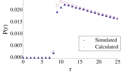
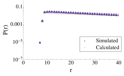
Figure 20: (Color online) Plots of the simulations and Eq. (23) for $V=9$ and $p=0.1$ at a density of 0.02 on (a) a regular scale and (b) a semilog scale.

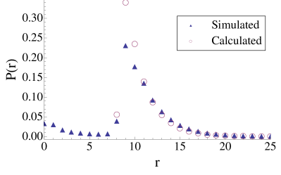
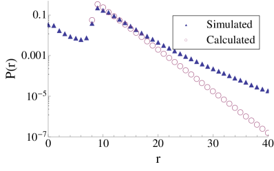
Figure 21: (Color online) Comparison of the simulations and the analytic prediction at a higher density of 0.09 for $V_{\text{max}}=9$ and $p=0.1$.

The speed distribution from Eq. (12) is then

$$P_{v}(m\!-\!2) = \alpha p$$

$$P_{v}(m\!-\!1) = (1-\alpha)p+\alpha(1-p)$$

$$P_{v}(m) = (1-\alpha)(1-p)\,,$$ (19)

where $\alpha=\Delta(m\!-\!1)$ is the fraction of cars with a gap of $V_{\text{max}}-1$. Putting this speed distribution into Eq. (14) with the assumed distribution for $f(v,g)$ given by Eqs. (17) and (18), we can produce an evolution equation for the gap distribution of the form

$$\Delta(g)_{t+1}=\sum_{g^{\prime}}\Gamma(g^{\prime}\to g)\Delta(g^{\prime})_{t}\,.$$

We find for $g\geq m+2$ that

$$\Delta(g)_{t+1}-\Delta(g)_{t} = A(\Delta(g\!-\!1)_{t}-\Delta(g)_{t})+$$ (20)

$$B(\Delta(g\!+\!1)_{t}-\Delta(g)_{t})+$$

$$C(\Delta(g\!+\!2)_{t}-\Delta(g)_{t})$$

$$\equiv \Phi[\Delta(g)]\,,$$

where $A=p^{\prime}(1-\alpha)$, $B=p^{\prime}+\alpha(1-3p^{\prime})$ and $C=\alpha p^{\prime}$, with $p^{\prime}=p(1-p)$. The evolution equations for smaller gaps are then

$$\Delta(m\!+\!1)_{t+1}\!-\!\Delta(m\!+\!1)_{t} = \Phi[\Delta(m\!+\!1)]+A\Delta(m\!-\!1)_{t}$$

$$\Delta(m)_{t+1}\!-\!\Delta(m)_{t} = \Phi[\Delta(m)]$$

$$+ (1\!-\!3p^{\prime}\!+\!\alpha(1\!-\!2p^{\prime}))\Delta(m\!-\!1)_{t}$$

$$\Delta(m\!-\!1)_{t+1} = \alpha\,.$$ (21)

In the continuum limit and for $g>m+1$, Eq. (20) becomes a drift-diffusion Fokker-Plank equation of the form

$$\frac{\partial\Delta}{\partial t}=\alpha\frac{\partial\Delta}{\partial g}+(p(1-p)+\alpha/2)\frac{\partial^{2}\Delta}{\partial g^{2}}\,,$$ (22)

for which the steady-state solution is of the form

$$\Delta(g)\propto\exp\left(-\frac{\alpha}{p(1-p)+\alpha/2}\,g\right)\,.$$ (23)

If we solve Eqs. (20) and (21) and compare them to our simulations, we see from Fig. 20 that the agreement is excellent except near the peak of the distribution. Since both distributions are normalized, the error at the peak results in slightly different slopes for large $g$. At higher densities, the agreement is not as good. Figure 21 shows the analytic description predicts the position of the peak at $g=V_{\text{max}}$, but the presence of the second jam phase in the simulations alters the distribution.

References

- Lighthill and Whitham (1955) M. J. Lighthill and G. B. Whitham, Proc. Roy. Soc. A, 229, 317 (1955).
- Prigogine and Herman (1971) I. Prigogine and R. Herman, Kinetic Theory of Vehicular Traffic (Elsevier, 1971).
- Chowdhury (2000) D. Chowdhury, Phys. Rep. 329, 199 (2000).
- Helbing (2001) D. Helbing, Rev. Mod. Phys. 73, 1067 (2001).
- Nagatani (2002) T. Nagatani, Rep. Prog. Phys. 65, 1331 (2002).
- Nagel and Schreckenberg (1992) K. Nagel and M. Schreckenberg, J. Phys. I 2, 2221 (1992).
- Nagel and Paczuski (1995) K. Nagel and M. Paczuski, Phys. Rev. E 51, 2909 (1995).
- Lübeck et al. (1998) S. Lübeck, M. Schreckenberg, and K. D. Usadel, Phys. Rev. E 57, 1171 (1998).
- Chowdhury et al. (1997) D. Chowdhury, K. Ghosh, A. Majumdar, S. Sinha, and R. B. Stinchcombe, Physica A 246, 471 (1997).
- Chowdhury et al. (1998) D. Chowdhury, A. Pasupathy, and S. Sinha, Eur. Phys. J. B 5, 781 (1998).
- Roters et al. (1999) L. Roters, S. Lübeck, and K. D. Usadel, Phys. Rev. E 59, 2672 (1999).
- Chowdhury et al. (2000) D. Chowdhury, J. Kertész, K. Nagel, L. Santen, and A. Schadschneider, Phys. Rev. E 61, 3270 (2000).
- Roters et al. (2000) L. Roters, S. Lübeck, and K. D. Usadel, Phys. Rev. E 61, 3272 (2000).
- Kerner et al. (2002) B. S. Kerner, S. L. Klenov, and D. E. Wolf, J. Phys. A-Math. Gen. 35, 9971 (2002).
- Vilar and Souza (1994) L. C. Q. Vilar and A. M. C. Souza, Physica A 211, 84 (1994).
- Jost and Nagel (2003) D. Jost and K. Nagel, Transport Res. Rec. 1852, 152 (2003).
- Miedema et al. (2014) D. M. Miedema, A. S. de Wijn, and P. Schall, Phys. Rev. E 89, 062812 (2014).
- Souza and Vilar (2009) A. M. C. Souza and L. C. Q. Vilar, Phys. Rev. E 80, 021105 (2009).
- Zhang et al. (2011) W. Zhang, W. Zhang, and W. Chen, e-print arXiv:1102.5704 [nlin.CG] (2011).
- Zhang and Zhang (2014) W. Zhang and W. Zhang, Eur. Phys. J. B 87, 4 (2014).
- de Wijn et al. (2012) A. S. de Wijn, D. M. Miedema, B. Nienhuis, and P. Schall, Phys. Rev. Lett. 109, 228001 (2012).
- Lakouari et al. (2014) N. Lakouari, K. Jetto, H. Ez-Zahraouy, and A. Benyoussef, Int. J. Mod. Phys. C 25, 1350089 (2014).
- Kerner (2013) B. S. Kerner, Physica A 392, 5261 (2013).
- Kerner et al. (2014) B. S. Kerner, S. L. Klenov, and M. Schreckenberg, Phys. Rev. E 89, 052807 (2014).
- Note (1) The gap between the cars is .
- Gerwinski and Krug (1999) M. Gerwinski and J. Krug, Phys. Rev. E 60, 188 (1999).
- Fisher (1967) M. E. Fisher, Rep. Prog. Phys. 30, 615 (1967).
- Barber (1983) M. N. Barber, in Phase Transitions and Critical Phenomena (Academic Press, London, 1983).
- Ferrenberg and Landau (1991) A. M. Ferrenberg and D. P. Landau, Phys. Rev. B 44, 5081 (1991).
- Balouchi (2016) A. Balouchi, Ph.D. thesis, Louisiana State University (2016).
- Note (2) The expression for here is the equal time correlation used in Ref. de Wijn et al. (2012).