Turing Computation with
Recurrent Artificial Neural Networks

Abstract

We improve the results by Siegelmann & Sontag [1, 2] by providing a novel and parsimonious constructive mapping between Turing Machines and Recurrent Artificial Neural Networks, based on recent developments of Nonlinear Dynamical Automata. The architecture of the resulting R-ANNs is simple and elegant, stemming from its transparent relation with the underlying NDAs. These characteristics yield promise for developments in machine learning methods and symbolic computation with continuous time dynamical systems. A framework is provided to directly program the R-ANNs from Turing Machine descriptions, in absence of network training. At the same time, the network can potentially be trained to perform algorithmic tasks, with exciting possibilities in the integration of approaches akin to Google DeepMind’s Neural Turing Machines.

1 Introduction

The present work provides a novel and alternative approach to the one offered by Siegelmann and Sontag [1, 2] of mapping Turing machines to Recurrent Artificial Neural Networks (R-ANNs). Here we employ recent theoretical developments from symbolic dynamics enabling the mapping from Turing Machines to two-dimensional piecewise affine-linear systems evolving on the unit square, i.e. Nonlinear Dynamical Automata (NDA)[3, 4]. With this in place, we are able to map the resulting NDA onto a R-ANN, therefore providing an elegant constructive method to simulate a Turing machine in real time by a first-order R-ANN. There are two main advantages to the proposed approach. The first one is the parsimony and simplicity of the resulting R-ANN architecture in respect to previous approaches. The second one is the transparent relation between the network and its underlying piecewise affine-linear system. These two characteristics open the door to key future developments when considering learning applications (see Google DeepMind’s Neural Turing Machines[5] for a relevant example with promising future integration possibilities) – with the exciting possibility of a symbolic read-out of a learned algorithm from the network weights – and when considering extensions of the model to continuous dynamics, which could provide a theoretical basis to query the computational power of more complex neuronal models.

2 Methods

In this section we outline a mapping from Turing machines to R-ANNs. Our construction involves two stages. In the first stage a Generalized Shift [3] emulating a Turing Machine is built, and its dynamics encoded on the unit square via a procedure called Gödelization, defining a piecewise-affine linear map on the unit square, i.e. a NDA. In the second stage, the resulting NDA is mapped onto a first-order R-ANN. Next, the theoretical methods employed are discussed in detail.

2.1 Turing Machines

A Turing Machine [6] is a computing device endowed with a doubly-infinite one-dimensional tape (memory support with one symbol capacity at each memory location), a finite state controller and a read-write head that follows the instructions encoded by a $\delta$ transition function. At each step of the computation, given the current state and the current symbol read by the read-write head, the machine controller determines via $\delta$ the writing of a symbol on the current memory location, a shift of the read-write head to the memory location to the left ($\mathcal{L}$) or to the right ($\mathcal{R}$) of the current one, and the transition to a new state for the next computation step. At a computation step, the content of the tape together with the position of the read-write head and the current controller state define a machine configuration.

More formally, a Turing Machine is a 7-tuple $M_{\text{TM}}=(Q,\mathbf{N},\mathbf{T},q_{0},\sqcup,F,\delta)$, where $Q$ is a finite set of control states, $\mathbf{N}$ is a finite set of tape symbols containing the blank symbol $\sqcup$, $\mathbf{T}\subset\mathbf{N}\setminus\{\sqcup\}$ is the input alphabet, $q_{0}$ is the starting state, $F\subset Q$ is a set of ‘halting’ states and $\delta$ is a partial transition function, determining the dynamics of the machine. In particular, $\delta$ is defined as follows:

$$\delta:Q\times\mathbf{N}\rightarrow Q\times\mathbf{N}\times\{\mathcal{L},\mathcal{R}\}.$$ (1)

2.2 Dotted sequences and Generalized Shifts

A Turing machine configuration can be described by a bi-infinite dotted sequence on some alphabet $\mathbf{A}$; it can then be defined as:

$$s=\ldots d_{i_{-3}}d_{i_{-2}}d_{i_{-1}}.d_{i_{0}}d_{i_{1}}d_{i_{2}}\ldots,$$ (2)

where $l=\ldots d_{i_{-3}}d_{i_{-2}}$ describes the part of the tape on the left of the read-write head, $r=d_{i_{0}}d_{i_{1}}d_{i_{2}}\ldots$ describes the part on its right, $q=d_{i_{-1}}$ describes the current state of the machine controller, and the dot denotes the current position of the read-write head, i.e. the symbol to its right. The central dot splits the tape into two one-sided infinite strings $\alpha^{\prime},\beta$, where $\alpha^{\prime}$ is the left part of the dotted sequence in reverse order. The first symbol in $\alpha$ represents the current state of the Turing Machine, whereas the first symbol in $\beta$ represents the symbol currently under the controller’s head. The transition function $\delta$ can be straightforwardly extended to a function $\hat{\delta}$ operating on dotted sequences, so that $\hat{\delta}:\mathbf{A}^{\mathbb{Z}}\rightarrow\mathbf{A}^{\mathbb{Z}}$.

A Generalized Shift acts on dotted sequences, and is defined as a pair $M_{GS}=(\mathbf{A}^{\mathbb{Z}},\Omega)$, with $\mathbf{A}^{\mathbb{Z}}$ being the space of dotted sequences, $\Omega:\mathbf{A}^{\mathbb{Z}}\rightarrow\mathbf{A}^{\mathbb{Z}}$ defined by

$$\Omega(s)=\sigma^{F(s)}(s\oplus G(s))$$ (3)

with

$$F :\mathbf{A}^{\mathbb{Z}}\rightarrow\mathbb{Z}$$ (4)

$$G :\mathbf{A}^{\mathbb{Z}}\rightarrow\mathbf{A}^{e}$$ (5)

where $\sigma$ shifts the symbols to the left or to the right, or does not shift them at all, as determined by the function $F(s)$. In addition, the Generalized Shift can operate a substitution, with $G(s)$ being the function which substitutes a substring of length $e$ in the Domain of Effect (DoE) of $s$ with a new substring. Both the shift and the substitution are functions of the content of the Domain of Dependence (DoD), a substring of $s$ of length $\ell$.

A Turing Machine can be emulated by a Generalized Shift with $\mbox{DoD}=\mbox{DoE}=d_{i_{-2}}d_{i_{-1}}.d_{i_{0}}$ and the functions $F,G$ appropriately chosen such that $\Omega(s)=\hat{\delta}(s)$ for all $s$ (see [7] for a detailed exposition).

2.3 Gödel codes

Gödel codes (or Gödelizations) [8] map strings to numbers and, in particular, allow the mapping of the space of one-sided infinite sequences to the real interval $[0,1]$. Let $\mathbf{A}^{\mathbb{N}}$ be the space of one-sided infinite sequences over an alphabet $\mathbf{A}$, $s$ be an element of $\mathbf{A}^{\mathbb{N}}$, $r_{k}$ the $k$-th symbol in $s$, $\gamma:\mathbf{A}\rightarrow\mathbb{N}$ a one-to-one function associating each symbol in the alphabet $\mathbf{A}$ to a natural number, and $g$ the number of symbols in $\mathbf{A}$. Then a Gödelization is a mapping $\psi$ from $\mathbf{A}^{\mathbb{N}}$ to $[0,1]\subset\mathbb{R}$ defined as:

$$\psi(s):=\sum\limits_{k=1}^{\infty}\gamma(r_{k})g^{-k}.$$ (6)

Conveniently, Gödelization can be employed on a Turing machine configuration, represented as a dotted sequence $\alpha.\beta\in\mathbf{A}^{\mathbb{Z}}$. The Gödel encoding $\psi_{x}$ and $\psi_{y}$ of $\alpha^{\prime}$ and $\beta$ define a representation of $s$ $(\psi_{x}(\alpha^{\prime}),\psi_{y}(\beta))$ known as symbol plane or symbologram representation, which is contained in the unit square ${[0,1]}^{2}\subset\mathbb{R}^{2}$. The choice of encoding $\psi_{x}$ and $\psi_{y}$ to use on the machine configurations is arbitrary. Therefore, to enable the construction of parsimonious Nonlinear Dynamical Automata our encoding will assume that $\beta$ always contains tape symbols only, and that the first symbol of $\alpha^{\prime}$ is always a state symbol, the rest being tape symbols only. Based on these assumptions, the particular encoding is defined as:

$$\psi_{x}(\alpha^{\prime}) =\gamma_{q}(a_{1})n_{q}^{-1}+\sum\limits_{k=1}^{\infty}\gamma_{s}(a_{k+1})n_{s}^{-k}n_{q}^{-1},$$ (7)

$$\psi_{y}(\beta) =\sum\limits_{k=1}^{\infty}\gamma_{s}(b_{k})n_{s}^{-k},$$

with $n_{q}=\lvert Q\rvert$, i.e. the number of states in the Turing Machine, $n_{s}=\lvert\mathbf{N}\rvert$, i.e. the number of tape symbols in the Turing Machine, $\gamma_{q}$ and $\gamma_{s}$ enumerating $Q$ and $\mathbf{N}$ respectively, and with $a_{k}$ and $b_{k}$ being the $k$-th symbol in $\alpha^{\prime}$ and $\beta$ respectively.

2.3.1 Encoded Generalized Shift and affine-linear transformations

The substitution and shift operated by a Generalized Shift on a dotted sequence $s=\alpha.\beta$ can be represented as an affine-linear transformation on $(\psi_{x}(\alpha^{\prime}),\psi_{y}(\beta))$, i.e. the symbologram representation of $s$. In particular, a substitution and shift on a dotted sequence can be broken down into substitutions and shifts on its one-sided components. In the following, we will show how substitutions and shifts on a one-sided infinite sequence can be represented as affine-linear transformations on its Gödelization. These results will be useful in showing how the symbologram representation of a Generalized Shift leads to a piecewise affine-linear map on a rectangular partition of the unit square.
Let $s=d_{1}d_{2}d_{3}\ldots$ be a one-side infinite sequence on some alphabet $\mathbf{A}$. Substituting the $n$-th symbol in $s$ with $\hat{d}_{n}$ yields $\hat{s}=d_{1}\ldots d_{n-1}\hat{d}_{n}d_{n+1}\ldots$, so that

$$\psi(s) =\gamma(d_{1})g^{-1}+\ldots\gamma(d_{n-1})g^{-(n-1)}+\gamma(d_{n})g^{-n}+\gamma(d_{n+1})g^{n+1}+\ldots,$$

$$\psi(\hat{s}) =\gamma(d_{1})g^{-1}+\ldots\gamma(d_{n-1})g^{-(n-1)}+\gamma(\hat{d}_{n})g^{-n}+\gamma(d_{n+1})g^{n+1}+\ldots,$$

$$=\psi(s)-\gamma(d_{n})g^{-n}+\gamma(\hat{d}_{n})g^{-n}.$$

As the previous example illustrates, Gödelizing a sequence resulting from a symbol substitution is equivalent to applying an affine-linear transformation on the original Gödelized sequence. In particular, the parameters of the affine-linear transformation only depend on the position and identities of the symbols involved in the substitution. Shifting $s$ to the left by removing its first symbol or shifting it to the right by adding a new one yields respectively $s_{l}=d_{2}d_{3}d_{4}\ldots$ and $s_{r}=b\;d_{1}d_{2}d_{3}d_{4}\ldots$, where $b$ is the newly added symbol. In this case

$$\psi(s_{l}) =\gamma(d_{2})g^{-1}+\gamma(d_{3})g^{-2}+\gamma(d_{4})g^{-3}+\ldots$$

$$=g\psi(s)-\gamma(d_{1}),$$

and

$$\psi(s_{r}) =\gamma(b)g^{-1}+\gamma(d_{1})g^{-2}+\gamma(d_{2})g^{-3}+\gamma(d_{3})g^{-4}+\ldots$$

$$=g^{-1}\psi(s)+\gamma(b)g^{-1}.$$

Again, the resulting Gödelized shifted sequence can be obtained by applying an affine-linear transformation to the original Gödelized sequence.

2.4 Nonlinear Dynamical Automata

A Nonlinear Dynamical Automaton (NDA) is a triple $M_{NDA}=(X,P,\Phi)$, with $P$ being a rectangular partition of the unit square, that is

$$P=\{D^{i,j}\subset X|~{}1\leq i\leq m,\;1\leq j\leq n,\;m,n\in\mathbb{N}\},$$ (8)

so that each cell $D^{i,j}$ is defined as the cartesian product $I_{i}\times J_{j}$, with $I_{i},J_{j}\subset[0,1]$ being real intervals for each bi-index $(i,j)$, $D^{i,j}\cap D^{k,l}=\emptyset$ if $(i,j)\neq(k,l)$, and $\bigcup_{i,j}D^{i,j}=X$.
The couple $(X,\Phi)$ is a time-discrete dynamical system with phase space $X={[0,1]}^{2}\subset\mathbb{R}^{2}$ (i.e. the unit square) and with flow $\Phi:X\rightarrow X$, a piecewise affine-linear map such that $\Phi_{|D^{i,j}}:=\Phi^{i,j}$. Specifically, $\Phi^{i,j}$ takes the following form:

$$\Phi^{i,j}(\mathbf{x})=\left(\begin{array}[]{c}a^{i,j}_{x}\\ a^{i,j}_{y}\end{array}\right)+\left(\begin{array}[]{cc}\lambda^{i,j}_{x}&0\\ 0&\lambda^{i,j}_{y}\end{array}\right)\left(\begin{array}[]{c}x\\ y\end{array}\right).$$ (9)

The piecewise affine-linear map $\Phi$ also requires a switching rule $\Theta(x,y)\in\llbracket 1,m\rrbracket\times\llbracket 1,n\rrbracket$ to select the appropriate branch, and thus the appropriate dynamics, as a function of the current state. That is, $\Phi(x,y)=\Phi^{i,j}(x,y)\iff\Theta(x,y)=(i,j)$.

Each cell $D^{i,j}$ of the partition $P$ of the unit square can be seen as comprising all the Gödelized dotted sequences that contain the same symbols in the Domain of Dependence. That is, for a Generalized Shift simulating a Turing Machine, the first two symbols in $\alpha^{\prime}$ and the first symbol in $\beta$.
The unit square is thus partitioned in a number of $I$ intervals equal to $m=n_{q}n_{s}$, and one of $J$ intervals equal to $n=n_{s}$, with $n_{q}$ being the number of states in $Q$ and $n_{s}$ the number of symbols in $\mathbf{N}$, for a total of $n_{q}n_{s}^{2}$ cells. As each cell corresponds to a different Domain of Dependence of the underlying Generalized Shift in symbolic space, it is associated with a different affine-linear transformation representing the action of a substitution and shift in vector space. The transformation parameters $(a^{i,j}_{x},a^{i,j}_{y})$ and $(\lambda^{i,j}_{x},\lambda^{i,j}_{y})$ can be derived using the methods outlined in subsubsection 2.3.1.
Thus, a Turing Machine can be represented as a Nonlinear Dynamical Automaton by means of its Gödelized Generalized Shift representation.

3 NDAs to R-ANNs

The aim of the second stage of our methodology is to map the orbits of the NDA (i.e. $\Phi^{i,j}(x,y)$) to orbits of the R-ANN, which we will denote by $\zeta^{i,j}(x,y)$.

Let $\rho(\cdot)$ denote the proposed map. Its role is to encode the affine-linear dynamics at each $\Phi^{i,j}$ branch in the architecture and weights of the network, and emulate the overall dynamics $\Phi$ by suitably activating certain neural units within the R-ANN given the switching rule $\Theta$. Therefore, we generically define the proposed map as follows:

$$\zeta=\rho(\mathcal{I},\mathcal{A},\Phi,\Theta),$$ (10)

where $\mathcal{I}$ is the identity matrix mapping (identically) the initial conditions of the NDA to the R-ANN and $\mathcal{A}$ is the adjacency matrix specifying the network architecture and weights, which will be explained in subsequent sections. In addition, $\rho$ defines different neural dynamics for each type of the neural units, that is, $\zeta=(\zeta_{1},\zeta_{2},\zeta_{3})$ corresponding to MCL, BSL and LTL, respectively (see below for the definitions of these acronyms). The details of the R-ANN architecture and its dynamics are subsequently discussed.

3.1 Network architecture and neural dynamics

The proposed map, $\rho$, attempts to mirror the affine-linear dynamics (given by Equation 9) of an NDA on the partitioned unit square (see Equation 8) by endowing the R-ANN with a structure capturing the characteristic features of a piecewise-affine linear system, i.e. a state, a switching rule and a set of transformations.
To achieve this, we propose a network architecture with three layers, namely a Machine Configuration Layer (MCL) encoding the state, a Branch Selection Layer (BSL) implementing the switching rule and a Linear Transformation Layer (LTL), as depicted in Figure 1.
The neural units within the various layers make use of either the Heaviside ($H$) or the Ramp ($R$) activation functions defined as follows:

$$H(x)=\begin{cases}0&\mbox{if }x<0\\ 1&\mbox{if }x\geq 0\\ \end{cases}$$ (11)

$$R(x)=\begin{cases}0&\mbox{if\;}x<0\\ x&\mbox{if\;}x\geq 0\\ \end{cases}.$$ (12)

Since $\Phi$ is a two-dimensional map, this suggests only two neural units ($c_{x},c_{y}$) in the MCL layer encoding its state at every step. A set of BSL units functionally acts as a switching system that determines in which cell $D^{i,j}$ the current Turing machine configuration belongs to and then triggers the specific LTL unit emulating the application of an affine-linear transformation $\Phi^{i,j}$ on the current state of the system. The result of the transformation is then fed back to the MCL for the next iteration. On the symbolic level, one iteration of the emulated NDA corresponds to a tape and state update of the underlying Turing machine, which can be read out by decoding the activation of the MCL neurons.

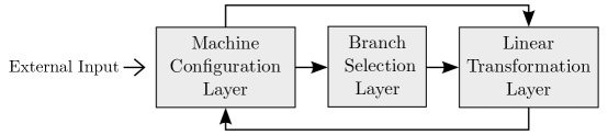
Figure 1: Connectivity between neural layers within the network.

3.1.1 Machine Configuration Layer

The role of the MCL is to store the current Gödelized configuration of the simulated Turing Machine at each computation step, and to synaptically transmit it to the BSL and LTL layers. The layer comprises two neural units ($c_{x}$ and $c_{y}$), as needed to store the Gödelized dotted sequence representing a Turing Machine configuration (see Equation 7).

The R-ANNs is thus initialized by activating this layer, given the NDA initial conditions $(\psi_{x}(\alpha^{\prime}),\psi_{x}(\beta))$ which are identically transformed via $\mathcal{I}$ by the map $\rho(\cdot)$ as follows:

$$(c_{x},c_{y})=(\psi_{x}(\alpha^{\prime}),\psi_{x}(\beta))\equiv\zeta_{1}=\rho(\mathcal{I},\cdot,\cdot,\cdot)_{|(\psi_{x}(\alpha^{\prime}),\psi_{x}(\beta))}$$ (13)

At each iteration, the units in this layer receive input from the LTL units, and are activated via the ramp activation function (Equation 12); in other words $\zeta_{1}\equiv(c_{x},c_{y})=(R(\sum_{i}t^{i}_{x}),R(\sum_{j}t^{j}_{y})$). Finally, the MCL synaptically projects onto the BSL and LTL (refer to Figure 2 for details of the connectivity).

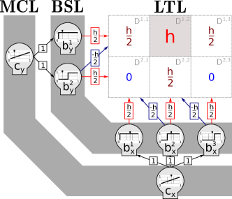
(a) Branch Selection Layer

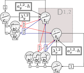
(b) Complete branch connection layout

Figure 2: Detailed feedforward connectivity and weights for a neural network simulating a NDA with only 6 branches.

3.1.2 Branch Selection Layer

The BSL embodies the switching rule $\Theta(x,y)$ and coordinates the dynamic switching between LTL units. In particular, if at the current step the MCL activation is $(c_{x},c_{y})\in D^{i,j}=I_{i}\times J_{j}$, with $I_{i}=[\xi_{i},\xi_{i+1})$ being the $i$-th interval on the $x$-axis and $J_{j}=[\eta_{j},\eta_{j+1})$ being the $j$-th interval on the $y$-axis, the BSL units activate only the $(t^{i,j}_{x},t^{i,j}_{y})$ units in the LTL. In this way, only one couple of LTL units is active at each step. The switching rule is mapped by $\rho(\cdot)$ as follows:

$$\zeta_{2}(x,y)=\rho(\cdot,\cdot,\cdot,\Theta(x,y)=(i,j)).$$ (14)

The BSL is composed of two groups of Heaviside (Equation 11) units, implementing respectively the $x$ and the $y$ component of the switching rule of the underlying piecewise affine-linear system, namely: i) the $b_{x}$ group receives input with weight $1$ from the $c_{x}$ unit of the MCL layer, and comprises $n_{q}n_{s}$ units (i.e. $b^{i}_{x},1\leq i\leq n_{q}n_{s}$); ii) the $b_{y}$ group receives input with weight $1$ from $c_{y}$ and comprises $n_{s}$ units (i.e. $b^{j}_{y},1\leq i\leq n_{s}$). The activation of the two groups of units is defined as:

$$b_{x}^{i} =H(c_{x}-\xi^{i})\quad \quad\xi^{i} =\min(I_{i}),$$ with (15)

$$b_{y}^{j} =H(c_{y}-\eta^{j})\quad \quad\eta^{j} =\min(J_{i}).$$ with

Each $b_{x}^{i}$ and $b_{y}^{j}$ BSL unit has an activation threshold, defined as the left boundary of the $I_{i}$ and $J_{j}$ intervals, respectively, and implemented as input from an always-active bias unit (with weight $-\xi^{i}$ for the $b_{x}^{i}$ unit and $-\eta^{j}$ for $b_{y}^{j}$). Therefore, an activation of $(c_{x},c_{y})$ in the MCL corresponding to a point on the unit square belonging to cell $D^{i,j}$, would trigger active all units $b_{x}^{k}$ with $k\leq i$. The same would occur for all neural units $b_{y}^{k}$ with $k\leq j$.

Each $b_{x}^{i}$ unit establishes synaptic excitatory connections (with weight $\frac{h}{2}$) to all LTL units corresponding to cells $D^{k,i}$ (i.e. $(t_{x}^{k,i},t_{y}^{k,i})$) and inhibitory connections (with weight $\frac{-h}{2}$) to all LTL units corresponding to cells $D^{k,i-1}$ (i.e. $(t_{x}^{k,i-1},t_{y}^{k,i-1})$), with $k=1,\ldots,n_{s}$; for a graphical representation see Figure 2. Similarly, each $b_{y}^{j}$ unit establishes synaptic excitatory connections to all LTL units corresponding to cells $D^{j,k}$ and inhibitory connections to all LTL units corresponding to cells $D^{j-1,k}$, with $k=1,\ldots,n_{q}n_{s}$. Together, the $b^{i}_{x}$ and $b^{j}_{y}$ units completely counterbalance through their synaptic excitatory connections the natural inhibition (of bias $h$, which value and definition will be discussed in the following section) of the LTL units corresponding to cell $D^{i,j}$ (i.e. $(t_{x}^{i,j},t_{y}^{i,j})$).

In other words each couple of LTL units $(t_{x}^{i,i},t_{y}^{i,j})$ receives an input of $B_{x}^{i}+B_{y}^{j}$, defined as follows:

$$B_{x}^{i} = b_{x}^{i}\frac{h}{2}+b_{x}^{i+1}\frac{-h}{2},$$ (16)

$$B_{y}^{j} = b_{y}^{j}\frac{h}{2}+b_{y}^{j+1}\frac{-h}{2},$$

where the input sum

$$B_{x}^{i}+B_{y}^{j}=\begin{cases}h&\mbox{ if }(c_{x},c_{y})\in D_{i,j}\\ \frac{h}{2}&\mbox{ if }c_{x}\in I_{i},c_{y}\not\in J_{j}\quad\mbox{ or }\quad c_{x}\not\in I_{i},c_{y}\in J_{j}\\ 0&\mbox{ if }(c_{x},c_{y})\not\in D_{i,j}\end{cases}$$ (17)

only triggers the relevant LTL unit if it reaches the value $h$. That is, if $(c_{x},c_{y})\in D_{i,j}$ then $B_{x}^{i}+B_{y}^{j}=h$, and the pair $(t^{i,i}_{x},t^{i,j}_{y})$ is selected by the BSL units. Otherwise $(t^{i,i}_{x},t^{i,j}_{y})$ stays inactive as $B_{x}^{i}+B_{y}^{j}$ is either equal to $\frac{h}{2}$ or $0$, which is not enough to win the LTL pair natural inhibition. An example of this mechanism is shown in Figure 2 , where the LTL units in cell $D^{1,2}$ are activated via mediation of $b_{x}=\{b^{1}_{x},b^{2}_{x},b^{3}_{x}\}$ and $b_{y}=\{b^{1}_{y},b^{2}_{y}\}$. Here, both $b^{3}_{x}$ and $b^{2}_{y}$ are not excited since $c_{x}$ and $c_{y}$, respectively, are not activated enough to drive them towards their threshold. However, $b_{x}^{2}$ excites (with weights $\frac{h}{2}$) the LTL units in cell $D^{2,2}$ and $D^{1,2}$ and inhibits (with weights $\frac{-h}{2}$) the LTL units in cell $D^{2,1}$ and $D^{1,1}$. Equally, $b_{y}^{2}$ excites (with weights $\frac{h}{2}$) the LTL units in cell $D^{2,1}$, $D^{2,2}$ and $D^{2,3}$ and inhibits (with weights $\frac{-h}{2}$) the LTL units in cells $D^{1,1}$, $D^{1,2}$ and $D^{1,3}$. The $b_{x}^{1}$ and $b_{y}^{1}$ units excite cells $\{D^{2,1},D^{1,1}\}$ and $\{D^{1,1},D^{1,2},D^{1,3}\}$, respectively, but these do not inhibit any cells (due to boundary conditions).

3.1.3 Linear Transformation Layer

The LTL layer can be functionally divided in sets of two units, where each couple applies two decoupled affine-linear transformations corresponding to one of the branches of the simulated NDA. On the symbolic level, this endows the LTL with the ability to generate an updated machine configuration from the previous one. In the LTL, a branch $(i,j)$ of a NDA, $\Phi^{i,j}(x,y)=(\lambda^{i,j}_{x}x+a^{i,j}_{x},\lambda^{i,j}_{y}y+a^{i,j}_{y})$, is simulated by the LTL units $(t^{i,j}_{x},t^{i,j}_{y})$. Mathematically, this induces the following mapping:

$$(t^{i,j}_{x},t^{i,j}_{y}) = \zeta_{3}^{i,j}(x,y)=\rho(\cdot,\cdot,\Phi^{i,j}(x,y),\cdot).$$ (18)

The affine-linear transformation is implemented synaptically, and it is only triggered when the BSL units provide enough excitation to enable $(t^{i,j}_{x},t^{i,j}_{y})$ to cross their threshold value and execute the operation. The read-out of this process corresponds to:

$$\begin{array}[]{lcl}t^{i,j}_{x}&=&R(\lambda^{i,j}_{x}c_{x}+a^{i,j}_{x}-h+B_{x}^{i}+B_{y}^{j}),\\ t^{i,j}_{y}&=&R(\lambda^{i,j}_{y}c_{y}+a^{i,j}_{y}-h+B_{x}^{i}+B_{y}^{j}).\end{array}$$ (19)

A strong inhibition bias $h$ (implemented as a synaptic projection from a bias unit) plays a key role in rendering the LTL units inactive in absence of sufficient excitation. The bias value is defined as follows

$$-\frac{h}{2}\leq-\max_{i,j,k}(a^{i,j}_{k}+\lambda^{i,j}_{k})\quad\text{with}\quad k=\{x,y\}.$$ (20)

Hence, each of the BSL inputs $B^{i}_{x}$ and $B^{i}_{y}$ contributes respectively to half of the necessary excitation ($\frac{h}{2}$) needed to counterbalance the LTL’s natural inhibition (refer to Equation 16 and Equation 17).

The LTL units receive input from the two CSL units $(c_{x},c_{y})$, with synaptic weights of $(\lambda^{i,j}_{x},\lambda^{i,j}_{y})$, and they are also endowed with an intrinsic constant LTL neural dynamics $(a^{i,j}_{x},a^{i,j}_{y})$. If the input from the BSL layer is enough for these neurons to cross the threshold mediated by the Ramp activation function, the desired affine-linear transformation is applied. The read-out is an updated encoded Turing machine configuration, which is then synaptically fed back to the CSL units $(c_{x},c_{y})$, ready for the next iteration (or next Turing machine computation step on the symbolic level).

3.1.4 NDA-simulating first order R-ANN

The NDA simulation (and thus Turing machine simulation) by the R-ANN is achieved by a combination of synaptic and neural computation among the three neural types (MCL, BSL, and LTL) and with a total of

$$n_{\text{units}}=\underbrace{\vphantom{n_{q}}2}_{\text{MCL}}+\underbrace{n_{s}+n_{s}n_{q}}_{\text{BSL}}+\underbrace{2n^{2}_{s}n_{q}}_{\text{LTL}}+\underbrace{\vphantom{n_{q}}1}_{\text{bias unit}}$$ (21)

neural units, where $n_{q}$ and $n_{s}$ are the number of states and the number of symbols in the Turing Machine to be simulated, respectively. These units are connected as specified by an adjacency matrix $\mathcal{A}$ of size $n_{\text{units}}\times n_{\text{units}}$, following the connectivity pattern described in Figure 1 and with synaptic weights as entries from the set

$$\{0,1,\frac{h}{2},\frac{-h}{2}\}\cup\{a^{i,j}_{k}-h\;|\;i=1,\ldots,n_{q}n_{s}\enskip,\enskip j=1,\ldots,n_{s}\enskip,\enskip k=x,y\},$$

the second component being the set of biases.

An important modelling issue to consider is that of the halting conditions for the ANN, i.e. when to consider the computation completed. In the original formulation of the Generalized Shift, there is no explicit definition of halting condition. As our ANN model is based on this formulation, a deliberate choice has to be made in its implementation. Two choices seem to be the most reasonable. The first one involves the presence of an external controller halting the computation when some conditions are met, i.e. an homunculus [4]. The second one is the implementation of a fixed point condition, intrinsic to the dynamical system, representing a TM halting state as an Identity branch on the NDA. In this way a halting configuration will result in a fixed point on the NDA, and thus on the R-ANN. In other words, the network’s computation is considered completed if and only if

$$\zeta_{1}(x^{\prime},y^{\prime})=(x^{\prime},y^{\prime}).$$ (22)

In the present study we decided to use a fixed point halting condition, but the use of a homunculus would likely be more appropriate in other contexts such as interactive computation [9, 10, 11] or cognitive modelling, where different kinds of fixed points are required in order to describe sequential decision problems [12], such as linguistic garden paths [4, 10].

The implementation of the R-ANN defined like so simulates a NDA in real-time and, thus, it simulates a Turing Machine in real time. More formally, it can be shown that under the map $\rho(\cdot)$ the commutativity property $\zeta\circ\rho=\rho\circ\Phi$ is satisfied, which extends the previously demonstrated commutativity property between Turing machines and NDAs [9, 13, 14].

4 Discussion

In this study we described a novel approach to the mapping of Turing Machines to first-order R-ANNs. Interestingly, R-ANNs can be constructed to simulate any piecewise affine-linear system on a rectangular partition of the $n$-dimensional hypercube by extending the methods discussed

The proposed mapping allows the construction, given any Turing Machine, of a R-ANN simulating it in real time. As an example of the parsimony we claim, a Universal Turing Machine can be simulated with a fraction of the units than previous approaches allowed for: the proposed mapping solution derives a R-ANN that can simulate Minsky’s 7-states 4-symbols UTM [15] in real-time with 259 units (as per Equation 21), approximately 1/3 of the 886 units needed in the solution proposed by Siegelmann and Sontag [1], and with a much simpler architecture.

In future work we plan to overcome some of the issues posed by the mapping and parts of its underlying theory, especially in relation to learning applications. Key issues to overcome are the missing end-to-end differentiability, and the need for a de-coupling of states and data in the encoding. A future development would see the integration of methods of data access and manipulation akin to that in Google DeepMind’s Neural Turing Machines [5]. A parallel direction of future work would see the mapping of Turing machines to continuous-time dynamical systems (an example with polynomial systems is provided in [16]). In particular, heteroclinic dynamics  [12, 13, 17, 18] – with machine configurations seen as metastable states of a dynamical system – and slow-fast dynamics [19, 20] are promising new directions of research.

References

References

- [1] H. T. Siegelmann and E. D. Sontag, “On the computational power of neural nets,” Journal of computer and system sciences, vol. 50, no. 1, pp. 132–150, 1995.
- [2] H. T. Siegelmann and E. D. Sontag, “Turing computability with neural nets,” Appl. Math. Lett, vol. 4, no. 6, pp. 77–80, 1991.
- [3] C. Moore, “Unpredictability and undecidability in dynamical systems,” Physical Review Letters, vol. 64, no. 20, p. 2354, 1990.
- [4] P. beim Graben, B. Jurish, D. Saddy, and S. Frisch, “Language processing by dynamical systems,” International Journal of Bifurcation and Chaos, vol. 14, no. 02, pp. 599–621, 2004.
- [5] A. Graves, G. Wayne, and I. Danihelka, “Neural turing machines,” arXiv preprint arXiv:1410.5401, 2014.
- [6] A. M. Turing, “On computable numbers, with an application to the entscheidungsproblem,” Proc. London Math. Soc, vol. 42, 1937.
- [7] C. Moore, “Generalized shifts: unpredictability and undecidability in dynamical systems,” Nonlinearity, vol. 4, no. 2, p. 199, 1991.
- [8] K. Gödel, “Über formal unentscheidbare sätze der principia mathematica und verwandter systeme i,” Monatshefte für Mathematik und Physik, vol. 38, pp. 173 – 198, 1931.
- [9] P. beim Graben, “Quantum Representation Theory for Nonlinear Dynamical Automata,” in Advances in Cognitive Neurodynamics ICCN 2007, pp. 469–473, Springer, 2008.
- [10] P. beim Graben, S. Gerth, and S. Vasishth, “Towards dynamical system models of language-related brain potentials,” Cognitive neurodynamics, vol. 2, no. 3, pp. 229–255, 2008.
- [11] P. Wegner, “Interactive foundations of computing,” Theoretical Computer Science, vol. 192, pp. 315 – 351, 1998.
- [12] M. I. Rabinovich, R. Huerta, P. Varona, and V. S. Afraimovich, “Transient cognitive dynamics, metastability, and decision making,” PLoS Computational Biology, vol. 4, no. 5, p. e1000072, 2008.
- [13] P. beim Graben and R. Potthast, “Inverse problems in dynamic cognitive modeling,” Chaos: An Interdisciplinary Journal of Nonlinear Science, vol. 19, no. 1, p. 015103, 2009.
- [14] P. beim Graben and R. Potthast, “Universal neural field computation,” in Neural Fields, pp. 299–318, Springer, 2014.
- [15] M. Minsky, “Size and structure of universal turing machines using tag systems,” in Recursive Function Theory: Proceedings, Symposium in Pure Mathematics, vol. 5, pp. 229–238, 1962.
- [16] D. S. Graça, M. L. Campagnolo, and J. Buescu, “Computability with polynomial differential equations,” Advances in Applied Mathematics, vol. 40, no. 3, pp. 330–349, 2008.
- [17] I. Tsuda, “Toward an interpretation of dynamic neural activity in terms of chaotic dynamical systems,” Behavioral and Brain Sciences, vol. 24, pp. 793 – 810, 2001.
- [18] M. Krupa, “Robust heteroclinic cycles,” Journal of Nonlinear Science, vol. 7, no. 2, pp. 129–176, 1997.
- [19] M. Desroches, M. Krupa, and S. Rodrigues, “Inflection, canards and excitability threshold in neuronal models,” Journal of mathematical biology, vol. 67, no. 4, pp. 989–1017, 2013.
- [20] M. Desroches, A. Guillamon, R. Prohens, E. Ponce, S. Rodrigues, and A. E. Teruel, “Canards, folded nodes and mixed-mode oscillations in piecewise-linear slow-fast systems,” SIAM Review, vol. in press, 2015.