Influence of the nonlinearity parameter on the solar-wind sub-ion magnetic energy spectrum: FLR-Landau fluid simulations

Abstract

The cascade of kinetic Alfvén waves (KAWs) at the sub-ion scales in the solar wind is numerically simulated using a fluid approach that retains ion and electron Landau damping, together with ion finite Larmor radius corrections. Assuming initially equal and isotropic ion and electron temperatures, and an ion beta equal to unity, different simulations are performed by varying the propagation direction and the amplitude of KAWs that are randomly driven at a transverse scale of about one fifth of the proton gyroradius in order to maintain a prescribed level of turbulent fluctuations. The resulting turbulent regimes are characterized by the nonlinearity parameter, defined as the ratio of the characteristic times of Alfvén wave propagation and of the transverse nonlinear dynamics. The corresponding transverse magnetic energy spectra display power laws with exponents spanning a range of values consistent with spacecraft observations. The meandering of the magnetic field lines together with the ion temperature homogenization along these lines are shown to be related to the strength of the turbulence, measured by the nonlinearity parameter. The results are interpreted in terms of a recently proposed phenomenological model where the homogenization process along field lines induced by Landau damping plays a central role.

1 Introduction

An important issue when studying turbulence in the solar wind concerns the energy spectrum $E(k_{\perp})$ of the transverse magnetic fluctuations at sub-ion scales. Spacecraft observations reveal a power law in a range of scales extending roughly to the electron gyroscale $\rho_{e}$ (Alexandrova et al., 2008, 2013; Bruno & Carbone, 2013), but the question arises of the universality of the spectral exponent (Sahraoui et al., 2009, 2010, 2011; Alexandrova et al., 2012; Chen et al., 2013). Observational values reported in Fig. 5 of Sahraoui et al. (2013) are distributed within an interval $[-3.1,-2.5]$ with a peak of probability near $-2.8$, a range whose extension significantly exceeds the dispersion usually reported for the MHD-range spectral exponent, evaluated for example as $-1.63\pm 0.14$ in Smith et al. (2006). It turns out that, in some instances, the MHD and sub-ion ranges are separated by a short “transition range” located near the proton gyroscale $\rho_{i}$ where the spectrum displays a power-law with an exponent close to $-4$. The origin of this range is not fully understood, although the effect of monochromatic waves and coherent structures such as Alfvén vortices has recently been suggested (Alexandrova & Lion, private communication).

Clearly, the power-law observed for the transverse magnetic energy spectrum at the sub-ion scales is steeper than the $k_{\perp}^{-7/3}$ prediction obtained by assuming a purely inertial cascade and adapting to the ion scales the critical balance argument (Goldreich & Shridhar, 1995; Nazarenko & Schekochihin, 2011) that leads to the $k_{\perp}^{-5/3}$ spectrum in the MHD range. Although it cannot be completely excluded that the observed variations of the spectral index originate from difficulties in the use of the Taylor hypothesis (on which most of the analysis of observational data are based) beyond the ion scales, or from a possible influence of the solar wind velocity and of its angle with the ambient field (Sahraoui & Huang, private communication), we shall here focus on physical processes amenable to numerical simulations in the framework of fully kinetic descriptions or suitable fluid models.

Gyrokinetic simulations presented in Howes et al. (2011b) display a sub-ion magnetic energy spectrum exponent very close to the $-2.8$ most probable value reported from solar wind observations. A more recent simulation performed with a different code shows a $-3.1$ sub-ion range (Told et al., 2015). Although retaining only the low-frequency dynamics, such simulations require huge computational resources, making a parametric study difficult.

On the other hand, reduced fluid models, assuming isothermal ions and electrons, lead to a $k_{\perp}^{-8/3}$ spectrum, where the departure from the $-7/3$ exponent has been related to intermittency corrections originating from coherent structures (Boldyrev & Perez, 2012; Boldyrev et al., 2013). A $-8/3$ exponent is also obtained in numerical simulations of electron-MHD in the presence of a strong ambient field (Meyrand & Galtier, 2013). In addition, energy spectra steeper than $-7/3$, associated with coherent structures and deformation of the particle distribution functions, are reported from fully kinetic particle-in-cell (PIC) simulations with a reduced mass ratio (Wan et al., 2015), and from hybrid Eulerian Vlasov-Maxwell models (Servidio et al., 2015).

It turns out that, as the cascade proceeds, kinetic Alfvén waves (KAWs) become compressible, making Landau damping relevant. A phenomenological model was presented in Howes et al. (2008, 2011a) where, due to this effect, the cascade is non conservative and the energy flux decays exponentially as the cascade proceeds. This leads to an exponential multiplicative correction to the $k^{-7/3}$ spectrum which, under specific choices of parameters, can indeed look like a steeper power law. The intrinsic non-universality of the observed power-law energy spectrum is however not really reproduced. This model was recently revisited in Passot & Sulem (2015) by noting that Landau damping does not only lead to dissipation of the wave energy along the cascade but also induces a homogenization process of fields such as the temperatures along the distorted magnetic field lines, which affects the characteristic transfer time and thus the energy cascade. It in particular modifies the power-law exponent that appears to be sensitive to the nonlinearity parameter defined as the ratio of the Alfvén wave period to the nonlinear stretching time. Non-universality due to Landau damping was also reported in three-dimensional PIC simulations of whistler turbulence (Gary et al., 2012), and in fact turns out to be a generic property of systems for which the characteristic times of dissipation and transfer display the same variation in terms of the wavenumber (Bratanov et al., 2013).

The aim of the present paper is to address the question of the non-universality of the sub-ion magnetic energy spectrum for a proton-electron plasma with initially equal and isotropic equilibrium mean temperatures, using numerical simulations of the FLR-Landau fluid described in Sections 2 and 5 of Sulem & Passot (2015) (and references therein). The paper is organized as follows. In Section 2, we briefly review the main features of the FLR-Landau fluid model and specify the numerical setting. Section 3 discusses diagnostic tools. The main results are presented in Section 4 which, on the basis of FLR-Landau fluid numerical simulations, correlates the sub-ion exponent of the transverse magnetic spectrum to the nonlinearity parameter. Section 5 analyzes the meandering of magnetic field lines in various turbulence regimes. Section 6 provides an interpretation of the numerical observations, based on a recently developed phenomenological model (Passot & Sulem, 2015). An important ingredient of this latter approach is the homogenization process along the magnetic field lines of quantities such as the temperatures, which, in the case of ions but not of electrons, is supposed to affect the energy transfer. Section 7 demonstrates that this homogenization effect is indeed captured in the numerical simulations. Section 8 is the Conclusion.

2 The FLR-Landau fluid

2.1 Main features of the model

The FLR-Landau fluid model appears as a system of dynamical equations for the proton density and velocity, the magnetic field, the ion and electron parallel and perpendicular gyrotropic pressures and heat fluxes. The electric field is given by a generalized Ohm’s law which includes the Hall term and the electron pressure gradient, but neglects electron inertia. The fluid hierarchy is closed by expressing the gyrotropic fourth-rank moments in terms of the above quantities, in a way consistent with the low-frequency linear kinetic theory. It in particular retains Landau damping and finite Lamor radius (FLR) corrections (originating from the non-gyrotropic parts of the fluid moments and evaluated algebraically in terms of the retained quantities), leading to an accurate description of the dispersion and dissipation of KAWs.

It is of interest at this point to give a flavor of the way Landau damping is retained in such a fluid model. A main assumption is that, up to the distortion of the magnetic field lines that is taken into account, Landau damping keeps the same form as in the linear regime, an hypothesis probably valid when the turbulence fluctuations are not too strong (Kanekar et al., 2015). Although the present simulations involve a closure of the hierarchy at the level of the fourth-rank moments in order to retain a nonlinear dynamics for the gyrotropic heat fluxes and also to provide a better description of Landau damping in the nonlinear regime (see Schekochihin et al. (2015) for a discussion), the physical interpretation is easier in the simplified framework where the closure is done at the level of the heat fluxes. The equations for ion and electron gyrotropic pressures involve terms of the form $\nabla\cdot(q{\widehat{\mathbf{b}}})$ where $q$ is the parallel or perpendicular heat flux for the ions or the electrons, and ${\widehat{\mathbf{b}}}$ the unit vector parallel to the local magnetic field. In a magnetized weakly collisional plasma, each of the gyrotropic heat fluxes is modeled as $q\sim{\widehat{\mathbf{b}}}\cdot\nabla{\widetilde{T}}$ where ${\widetilde{T}}$ refers to the corresponding temperature fluctuations (Spitzer & Härm, 1953) Differently, in the collisionless regime, the heat flux scales like $v_{th}{\widetilde{T}}$ (Hollweg, 1974), where $v_{th}$ is the associated thermal velocity. Transition between these two regimes in the solar wind was recently studied both from observational data (Bale et al., 2013) and numerical simulations (Landi et al., 2014). The low-frequency linear kinetic theory reproduces this scaling, but the relation involves a Hilbert transform along the equilibrium magnetic field lines, making the system dissipative as a consequence of Landau damping (see e.g. Snyder et al. (1997)). In the nonlinear regime, as discussed in Passot et al. (2014), the distortion of the magnetic field lines is to be retained, requiring an approximation of the Hilbert transform along distorted lines. Substituting the resulting expressions for the heat fluxes into the pressure equations results in a homogenization process along the distorted magnetic lines, through the operator (having the dimension of an inverse time scale) $v_{th}{\widehat{b}}\cdot\nabla{\cal H}$ where ${\cal H}$ refers to the Hilbert transform along the magnetic field line (or in practice an approximation of it). The parallel or perpendicular ion or electron thermal velocity $v_{th}$ can be viewed as the rms particle streaming velocity and the operator $v_{th}{\mathbf{b}}\cdot\nabla$ phenomenologically associated with a homogenization frequency $\omega_{H}\sim v_{th}k_{\|}$, where $k_{\|}$ refers to an inverse correlation length along the magnetic field lines. One may thus expect that the streaming process is more efficient for the electrons than for the ions, and also when the strength of the turbulence (as measured by the nonlinearity parameter) is weaker, because the parallel wavenumber $k_{\|}$ is relatively smaller in this case, a point addressed in more details in Section 7.

2.2 Numerical setting

When numerically integrated, the FLR-Landau fluid equations given in Sulem & Passot (2015) are written in non-dimensional variables, using the Alfvén velocity $v_{A}$, the ion gyrofrequency $\Omega_{i}$ and the ambient magnetic field $B_{0}$ as basic units. Furthermore, weak linear hyper-viscosity and hyper-diffusivity terms are supplemented in the equations for the velocity and magnetic field components respectively. In the spectral space, these terms involve the same Fourier symbol $\nu(k_{z}^{8}+k_{\perp}^{8})$ where the coefficient $\nu$ is chosen as small as possible, while permitting the development of a small-scale fast-decaying range for the energy spectrum of the corresponding fields. These dissipative terms are added not only for preventing the development of numerical noise, but also to mimic the effect of the Landau dissipation at scales that are too small to be retained in the simulations. We checked that the resulting numerical dissipation is sufficiently small not to affect the power-law ranges. Terms corresponding to the work of the nongyrotropic pressure force are not retained in the equations for the ion parallel and perpendicular pressures. In a stationary regime where mean temperatures remain almost constant, these terms have a minor effect. Nevertheless, the resulting model is not exactly conservative, which does not appear to be a serious concern in situations involving both driving and numerical dissipation.

Run	$R_{0.2}^{80}$	$R_{0.13}^{80}$	$R_{0.08}^{80}$	$R_{0.08}^{83.6}$	$R_{0.08}^{86}$
$L_{\perp}/L_{\|}$	0.18	0.18	0.18	0.11	0.07
Propagation angle of injected KAWs	$80^{\circ}$	$80^{\circ}$	$80^{\circ}$	$83.6^{\circ}$	$86^{\circ}$
$\delta B_{\perp 0}/B_{0}={\langle|b_{\perp}|^{2}\rangle}^{1/2}$	0.2	0.13	0.08	0.08	0.08
$A=(k_{z}^{(0)}/k_{\perp}^{(0)})(B_{0}/\delta B_{\perp 0})$	0.9	1.38	2.25	1.38	0.88
Transverse magnetic spectrum exponent	-2.3	-2.6	-3.6	-2.8	-2.3

Table 1: Run parameters and spectral exponents. Here $k_{\perp}^{(0)}$ and $k_{z}^{(0)}$ are the transverse and parallel wavenumbers of the injected KAWs.

The FLR-Landau fluid equations are integrated using a Fourier pseudo-spectral method in a three-dimensional periodic domain, with a partial dealiasing ensured by spectral truncation at 2/3 of the maximal wavenumber in each coordinate direction. Parallelism is implemented using the so-called pencil decomposition. In order to focus on the quasi-transverse dynamics, the spatial extension of the domain is larger in the parallel direction than in the transverse ones. Time integration is performed with an explicit $3^{\rm rd}$-order Runge-Kutta scheme. A strong stability constraint on the time step originates from the use of a realistic ion-electron mass ratio, while long integration times (typically involving $10^{6}$ time steps) are needed to reach a stationary state and obtaining significant statistical quantities in this regime. For these reasons, the resolutions used at this stage were limited to $128^{3}$ or $256^{2}\times 128$ grid points.

In the present simulations where the smallest perpendicular wavenumber is $k_{\perp}d_{i}\approx 0.18$ (here $d_{i}$ denotes the ion inertial length), it is reasonable, when motivated by the solar wind physics, to look at the largest retained scales as produced by the MHD cascade, and thus to assume that they display a significant scale anisotropy. As solar wind turbulence dominantly involves Alfvénic fluctuations, we are led to include in the simulations, a driving that mimicks the injection of KAWs. For this purpose, we supplemented in the velocity equation a random forcing with components

$$F_{i}(t,\mathbf{x})=\sum_{1<n<N}F_{i,n}^{0}\ \cos(\omega_{{}_{KAW}}({\mathbf{k}}_{n})t-{\mathbf{k}}_{n}\cdot{\mathbf{x}}+\phi_{i,n}),$$ (1)

for different wavevectors ${\mathbf{k}}_{n}$, where $F_{i,n}^{0}$ and $\phi_{i,n}$ are the amplitude and phase of the $n^{th}$ mode of the $i^{th}$ component of the external driver $F_{i}$. When taking for $\omega_{{}_{KAW}}({\mathbf{k}})$ the KAW frequency at wavevector ${\mathbf{k}}$, the system will generate KAWs by resonance at this frequency. KAW frequencies are calculated from the linearized FLR-Landau fluid system, using a symbolic mathematics software. The dispersion relation is tabulated and used as an input in the FLR-Landau fluid code. Eight KAWs (four forward and four backward propagating waves with an orthogonal polarization) with wavevector components $(\pm 2\pi/L_{\perp},\pm 2\pi/L_{\perp})$ ,  $(\pm 2\pi/L_{\perp},\mp 2\pi/L_{\perp})$, $(0,\pm 2\pi/L_{\perp})$  and $(\pm 2\pi/L_{\perp},0)$ in the transverse spectral plane and  $\pm 2\pi/L_{\|}$ in the parallel direction (where $L_{\perp}$ and $L_{\|}$ refer to the dimensions of the computing box) are excited, those at the largest scales propagating in a direction making a prescribed angle with the ambient magnetic field, chosen from 80 to 86 degrees by varying $L_{\|}$. The driving is turned on (resp. off) when the sum of the kinetic and magnetic energies is below (resp. above) prescribed thresholds, taken such that the rms magnetic field fluctuations remain at a prescribed level (from 0.057 to 0.2). An alternative procedure, discussed in TenBarge et al. (2014) and implemented in gyrokinetic simulations (Howes et al., 2011b), consists in driving counterpropagating Alfvén waves by means of a parallel body current, using an oscillating antenna which obeys a Langevin equation.

Simulations were performed assuming initially equal isotropic ion and electron temperatures and $\beta=1$ for each particle species. We use a computational domain of transverse size $L_{\perp}=34.6\,d_{i}$, and different longitudinal extensions $L_{\|}$, leading to different propagation angles $\theta={\rm atan}(L_{\|}/L_{\perp})$ for the driven KAWs. The other parameter we vary is the rms amplitude of the transverse (normalized) magnetic fluctuations $a=\delta B_{\perp 0}/B_{0}$. These quantities enters the definition of $A=k_{z}^{(0)}/k_{\perp}^{(0)}(B_{0}/\delta B_{\perp 0})=(L_{\perp}/L_{\|})(B_{0}/\delta B_{\perp 0})$, a ratio of two quantities that are taken asymptotically small but of the same order in the gyrokinetic theory. Table 1 summarizes the parameters of the various simulations, referred to as $R_{a}^{\theta}$.

Due to the modest resolution of the present simulations, the retained wavenumbers in the transverse direction do not exceed a few $\rho_{i}^{-1}$. Nevertheless, as these simulations do no include a transition range which, as recalled in the Introduction, is not always observed in solar wind data, the power-laws for the transverse magnetic field obtained numerically can be viewed as characteristic of the sub-ion scales and extrapolated down to the electron gyroscale, thus permitting comparisons with the predictions of the phenomenological model introduced in Passot & Sulem (2015) and discussed in Section 6.

3 Diagnostic tools

3.1 Magnetic field lines

In addition to the usual Eulerian quantities, it is useful to consider individual field lines at a time when turbulence has reached a steady state. We considered 32 such lines originating from points distributed over an array of $8\times 4$ equispaced grid points in the range $10\leq x\leq 24$, $10\leq y\leq 24$, in the plane $z=0$. The magnetic field lines are computed by solving numerically the equation ${d{\mathbf{x}}}/{ds}={\widehat{\mathbf{b}}}({\mathbf{x}})$, where $s$ is the curvilinear abscissa along a field line, using a standard variable-order, variable-step Adams method. In order to make the computation of the field lines less time consuming, while keeping a reasonably good accuracy, we have adopted an approximate description of the magnetic field where only the Fourier modes of ${\mathbf{B}}$ with amplitude larger then $10^{-5}$ have been retained (Borgogno et al., 2008). This leads us to use of the order of $7\times 10^{4}$ to $10^{5}$ Fourier modes for each scalar component in the strong turbulence regime and about $10^{4}$ for weak turbulence.

3.2 Parallel wavenumber

An important issue, especially in the strong turbulence regime, is the distinction between the wavenumber $k_{z}$ along the uniform ambient magnetic field, and the quantity $k_{\|}$ arising in the nonlinear regime. While the former can just be viewed as a Fourier variable, the latter is rather defined as the inverse correlation length of the amplitude of the magnetic field fluctuations along the magnetic field lines and, as such, turns out to be a function of the considered transverse scale. This leads to define the quantity $k_{\|}(k_{\perp})$ for which a computation formula is given in Cho et al. (2002):

$$k_{\|}(k_{\perp})\approx\left(\frac{\sum_{k_{\perp}\leq k^{\prime}_{\perp}<k_{\perp}+\delta k_{\perp}}|\widehat{{\mathbf{B}}_{L}\cdot\nabla{\mathbf{b}}_{l}|^{2}_{\mathbf{k}^{\prime}}}}{B_{L}^{2}\sum_{k_{\perp}\leq k^{\prime}_{\perp}<k_{\perp}+\delta k_{\perp}}|\widehat{{\mathbf{b}}_{l}}|^{2}_{\mathbf{k}^{\prime}}}\right)^{1/2}.$$ (2)

In Eq. (2), ${\mathbf{B}}_{L}$ is the local mean field obtained by eliminating modes whose perpendicular wavenumber is greater than $k_{\perp}/2$, and ${\mathbf{b}}_{l}$ the fluctuating field obtained by eliminating modes whose perpendicular wavenumber is less than $k_{\perp}/2$. In order to reduce statistical fluctuations on the evaluation of $k_{\|}$ when turbulence has reached a steady state, averaging is performed over 70 to 200 outputs, depending on the conditions.

4 Nonlinearity parameter and spectral exponent

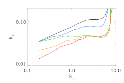
Figure 1: Parallel wavenumber $k_{\|}(k_{\perp})$ for runs $R_{0.2}^{80}$ (black), $R_{0.13}^{80}$ (blue), $R_{0.08}^{80}$ (green), $R_{0.08}^{83.6}$ (orange) and $R_{0.08}^{86}$ (red).

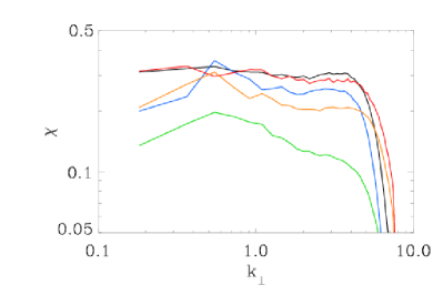
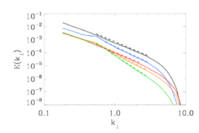
Figure 2: Nonlinearity parameter $\chi$ (top) and transverse magnetic energy spectrum $E(k_{\perp})$ (bottom) for the same runs as in Fig. 1 (same color code).

It is usually believed that strong turbulence in an anisotropic system in the presence of propagating waves is characterized by a “critical balance” condition where the characteristic times of the transverse nonlinear dynamics and of the wave propagation along the magnetic field lines display the same scaling in terms of the transverse wavenumber $k_{\perp}$. This leads to define a “nonlinearity parameter” $\chi=\omega_{NL}/\omega_{W}$ as the ratio of the associated frequencies. In the present situation where the turbulent cascade is dominated by the Alfvén wave dynamics, $\omega_{W}={\overline{\omega}}(k_{\perp}\rho_{i})k_{\|}v_{A}$. The function ${\overline{\omega}}$, which is provided by the linear kinetic theory, is equal to 1 at the MHD scales and varies like $k_{\perp}\rho_{i}$ when $k_{\perp}\rho_{i}\gg 1$. Furthermore, $\omega_{NL}$ corresponds to the rate of strain of the magnetic field by the electron velocity gradients. In the sub-ion range, electron velocity (which is significantly larger than ion velocity) scales approximately like the electric current. When the energy spectrum $E(k_{\perp})$ of the transverse magnetic fluctuations is sufficiently shallow for local interactions to be dominant (which turns out to be the case for $\beta$ of order unity), we estimate $\omega_{NL}\sim{\overline{\alpha}}[k_{\perp}^{3}E(k_{\perp})]^{1/2}$, where ${\overline{\alpha}}={\overline{\omega}}$. Modeling of non-local contributions is presented in Passot & Sulem (2015).

The longitudinal wavenumber $k_{\|}(k_{\perp})$, computed as indicated in Section 3.2, is displayed in Fig. 1 for the various simulations listed in Table 1. We note that in the case of run $R_{0.08}^{80}$, $k_{\|}$ is almost constant (down to the scales where hyperviscosity and hyperdiffusivity are significant and lead to a rapid increase), suggesting that this simulation corresponds to a weak turbulence regime. In contrast, for larger amplitude or larger propagation angle, $k_{\|}(k_{\perp})$ grows as a power law and saturates only at smaller scales.

Figure 2 (top) displays the nonlinearity parameter $\chi(k_{\perp})=(k_{\perp}^{3}E_{k})^{1/2}/k_{\|}(k_{\perp})v_{A}$ (assuming ${\overline{\alpha}}={\overline{\omega}}$), averaged over a time interval when the system has reached a stationary state, for the various runs listed in Table 1. Two types of behavior can be distinguished. In situations where the parameter $A$ is small, either because of a relatively large amplitude or a small ratio $L_{\|}/L_{\perp}$, the nonlinearity parameter $\chi(k_{\perp})$ is essentially constant, signature of a critically balanced turbulence. Differently, in simulations for which $A$ is larger, $\chi(k_{\perp})$ has a tendency to decrease.

Figure 2 (bottom) displays the corresponding transverse energy spectra of the transverse magnetic fluctuations, averaged on the same time interval as the nonlinearity parameter. If at the smallest scales the spectra rapidly decay due to the hyper-viscosity and hyperdiffusivity, one can clearly see a power-law behavior in the close sub-ion range, in spite of the moderate extension of this range due to numerical constraints. An important observation is that the spectral exponent is not universal, but turns out to be correlated with the saturated value of the nonlinear parameter: as the latter is larger, the spectrum is shallower.

In connection with the above result, a few comments are in order. A first remark is that no transition range is present in the simulations, suggesting that the same power-law spectrum extends from the ion to the electron gyroscale. Furthermore, a similar result is obtained by Gary et al. (2012) in numerical simulations of whistler waves for which the power-law spectrum at scales larger than the electron scales is reported to be shallower when, all other parameters being fixed, the turbulence energy flux is increased. On the other hand, apparently different conclusions have been drawn from solar wind observational data. Recently, Bruno et al. (2014) investigated the behavior of the spectral slope of interplanetary magnetic field fluctuations at proton scales from the WIND and MESSENGER spacecrafts at 1 AU and 0.56 AU, respectively, moving from fast to slow wind regions. They confirm the variability of the spectral slope, but exponents in the interval $-3.75$ to $-1.75$ are reported, with a tendency to approach $−5/3$ within the slowest wind, a value significantly in excess of theoretical and numerical predictions. They also observed a tendency for the spectrum to be steeper where the speed is higher, and to be flatter within the subsequent slower wind, following a gradual transition between these two states. They conclude that the value of the spectral index depends on the power associated with the fluctuations within the inertial range, the higher the power, the steeper the slope. Similar conclusions were reached by Smith et al. (2006). Comparisons with simulations where for example all the parameters are fixed except the amplitude of the turbulence fluctuations, is not straightforward. Indeed, as noted by Bruno et al. (2014), fluctuations within faster wind not only have larger amplitudes but are also more Alfvénic, i.e. display a larger cross-helicity. Furthermore, average values of the spectral index at proton scales, based on statistical studies employing a large data set, would depend on the relative amount of fast and slow wind present in the data set itself. Further analysis are needed for matching results of numerical simulations and observational data, mostly by making more specific the conditions in which the problem is addressed. It should in particular be stressed that, according to both the FLR-Landau fluid simulations and the phenomenological model, the turbulence state cannot be characterized by the sole amplitude of the turbulence fluctuations, but rather by the nonlinearity parameter which is however difficult to estimate from solar wind observations.

5 Magnetic field line meandering

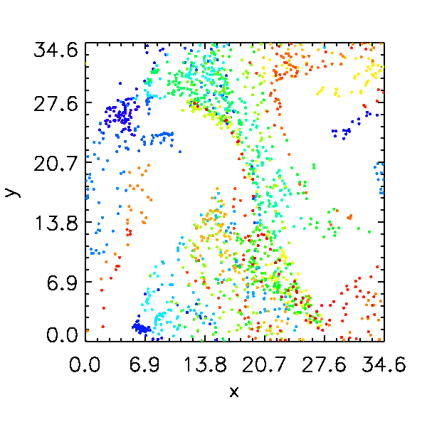
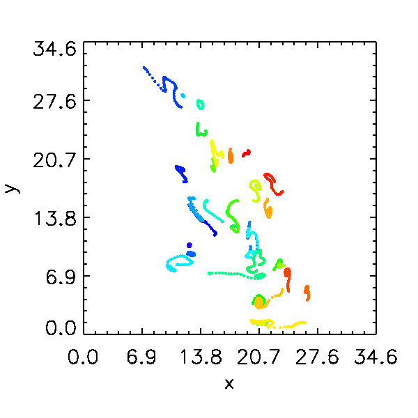
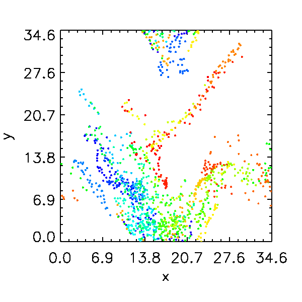
Figure 3: Poincaré map for runs $R_{0.2}^{80}$ (left), $R_{0.08}^{80}$ (middle) and $R_{0.08}^{86}$ in the transverse plane $z=L_{z}/2$, of 32 magnetic field lines originating from equidistributed points in a square of the plane $z=0$, whose linear dimensions are about $L_{\perp}/3$, at a time when turbulence has reached a stationary regime. Various colors correspond to the different field lines.

A main observation of Section 4 is that the strength of the turbulence and the spectral exponent at the sub-ion scales are governed by the nonlinearity parameter that itself results from the driving conditions, characterized by the parameter $A$ rather than by the amplitude of the turbulence fluctuations only. It is thus of interest to also analyze the influence of the parameter $A$ in physical space. For this purpose, we explore the magnetic field line properties at a given time when turbulence has reached a stationary state. Taking advantage of the periodicity of the computational domain, these (non periodic) lines are computed beyond the computational domain. Turbulence statistical homogeneity then allows one to explore various regions when integration is carried out on many spatial periods. It is then convenient to consider the Poincaré maps defined by the intersection points of the considered magnetic lines with a transverse plane, here chosen to be located at $z=L_{\|}/2$. These points can be viewed as the projections of the intersection points of the field lines with parallel transverse planes separated by a distance $L_{\|}$. The erratic character of the intersection points associated with a given line and the mixing of the different lines can then be viewed as reflecting the strength of the turbulence.

We have considered Poincaré maps for magnetic field lines corresponding to runs $R_{0.2}^{80}$, $R_{0.08}^{80}$ and $R_{0.08}^{86}$. The first two runs differ by the amplitude of the turbulent fluctuations, while the third one is characterized by the same level of fluctuations as the second one but has the same parameter $A$, and essentially the same nonlinearity parameter $\chi$, as the first one. Figure 3 displays the 50 intersections for the 32 considered magnetic lines (each of them characterized by a different color), in the three simulations. Interestingly, although they correspond to a different level of fluctuations, runs $R_{0.2}^{80}$ and $R_{0.08}^{86}$ (that display the same $\chi$) both display an erratic distribution of the intersection points of magnetic field lines in the transverse plane and a significant mixing of these lines, a situation that appears to be associated to a regime of strong turbulence. On the other hand, for run $R_{0.08}^{80}$ that corresponds to a regime of weak turbulence, the successive intersection points of individual field lines form distinct clusters, a configuration which is not significantly affected when increasing the extension of the considered field lines and thus the number of intersections. These observations indicate that the degree of meandering of the magnetic field lines is not associated with the amplitude of the turbulence fluctuations but rather to the value of the nonlinearity parameter, which governs the weak or strong character of the turbulence. This remark could be of interest in the context of propagation of solar energetic particles (SEP) for which the sole Fokker-Planck equation cannot explain the fast longitudinal diffusion (Latinen et al., 2015).

6 A phenomenological model

The non universality of the transverse energy spectrum of the magnetic fluctuations at the sub-ion scales and its sensitivity to the nonlinearity parameter, observed numerically with the FLR-Landau fluid, is also predicted by the phenomenological model presented in Passot & Sulem (2015), aimed at determining the stationary magnetic energy spectrum at scales smaller than the transition range if it exists. We here briefly review this model in the simpler situation where the nonlinear interactions are mostly local, which is the case for $\beta=1$ because the energy spectrum is not very steep. Ion and electron mean temperatures are assumed equal and isotropic.

In addition to the nonlinear frequency $\omega_{NL}=\Lambda[k_{\perp}^{5}\rho_{i}^{2}E_{k}]^{1/2}$ (here $\Lambda$ is a numerical constant of order unity, and $E_{k}$ holds for $E(k_{\perp}$)), and the frequency $\omega_{W}={\overline{\omega}}k_{\|}v_{A}$ (where ${\overline{\omega}}$ scales like $k_{\perp}\rho_{i}$) of KAWs propagating along the (distorted) magnetic field lines, additional characteristic time scales have to be considered. Landau resonance induces a damping rate, given by $\gamma={\overline{\gamma}}k_{\|}v_{A}$ where ${\overline{\gamma}}$ scales approximately like $k_{\perp}^{2}\rho_{i}^{2}$, at least for $\beta$ of order unity, but also a homogenization frequency $\omega_{H}=\mu k_{\|}v_{th}$ (where $\mu$ is a proportionality constant), which in the case of ions is comparable to the other inverse characteristic time scales. Due to the mass ratio, the corresponding frequency is much higher in the case of the electrons, making the homogenization of the electron along the magnetic field lines too fast for having a significant dynamical effect. This point will be addressed in the next section. The problem then arises of evaluating the characteristic transfer time, or its inverse $\omega_{tr}$. For this purpose, we proceed in the spirit of the classical two-point closures, such as the EDQNM model, classically used in hydrodynamic turbulence (Orszag, 1970, 1976; Sulem et al., 1975; Lesieur, 2008) and also in the context of homogeneous MHD where the influence of large-scale Alfvén wave on the inertial dynamics is to be retained (Pouquet et al., 1976). Details are given in the Appendix. One is led to write

$$\omega_{tr}=\frac{\omega_{NL}^{2}}{\omega_{W}+\omega_{H}}=\frac{\Lambda^{2}{\overline{\alpha}}^{2}k_{\perp}^{3}E_{k}}{{\overline{\omega}}v_{A}k_{\|}+\mu v_{th}k_{\|}}$$ (3)

where ${\overline{\alpha}}={\overline{\omega}}\sim k_{\perp}\rho_{i}$.

One can then define a turbulent energy flux by

$$\epsilon=C\omega_{tr}k_{\perp}E_{k},$$ (4)

where $C$ is a negative power of the Kolmogorov constant. Substituting Eq. (3) into Eq. (4), one gets

$$\epsilon=\frac{C\Lambda^{2}{\overline{\alpha}}^{2}k_{\perp}^{4}E_{k}^{2}}{({\overline{\omega}}v_{A}+\mu v_{th})k_{\|}}.$$ (5)

At scales for which $k_{\perp}\rho_{i}\gg 1$, determining $k_{\|}$ from the critical balance argument $\omega_{NL}\propto\omega_{W}$, it follows that, to leading order (taking, up to a simple rescaling, the corresponding proportionality constant equal to $\Lambda$ which then identifies with the nonlinearity parameter),

$$E_{k}\sim\Lambda^{-4/3}C^{-2/3}\epsilon^{2/3}k_{\perp}^{-7/3}.$$ (6)

Here, due to Landau damping, $\epsilon$ is a function of $k_{\perp}$ and decays along the cascade.

Indeed, retaining linear Landau damping leads to the phenomenological equation for KAW’s energy spectrum (Howes et al., 2008, 2011a)

$$\partial_{t}E_{k}+{\mathcal{T}}_{k}=-2\gamma E_{k}+S_{k},$$ (7)

where $S_{k}$ is the driving term acting at large scales and ${\mathcal{T}}_{k}$ the transfer term related to the energy flux $\epsilon$ by ${\mathcal{T}}_{k}=\partial\epsilon/\partial{k_{\perp}}$. Due to Landau damping, energy is not transferred conservatively along the cascade, making $\epsilon$ scale-dependent. For a steady state and outside the injection range, one has

$${d\epsilon}/{dk_{\perp}}=-2\gamma E_{k}\equiv-2{\overline{\gamma}}v_{A}k_{\|}E_{k},$$ (8)

where, using Eq. (5) (after multiplying the numerator and denominator of the RHS by $k_{\|}$),

$$k_{\|}E_{k}=\frac{C^{-1}\Lambda^{-2}}{k_{\perp}{\overline{\alpha}}^{2}v_{A}^{2}}({\overline{\omega}}v_{A}+\mu v_{th})\left(\frac{v_{A}^{2}k_{\|}^{2}}{k_{\perp}^{3}E_{k}}\right)\epsilon.$$ (9)

In a critically balanced regime, where $k_{\|}v_{A}=(k_{\perp}^{3}E_{k})^{1/2}$, Eq. (8) is then solved as

$$\epsilon=\epsilon_{0}\exp\left[-2C^{-1}\Lambda^{-2}\int_{k_{0}}^{k_{\perp}}\frac{{\overline{\gamma}}}{\xi{\overline{\alpha}}^{2}}({\overline{\omega}}+\mu\beta^{1/2})d\xi\right].$$ (10)

This (scale-dependent) energy flux is to be substituted in Eq. (6), using ${\overline{\alpha}}={\overline{\omega}}$ and ${\overline{\gamma}}/{\overline{\omega}}^{2}\approx\delta(\beta)$, which can be approximated by $0.78\rho_{e}/\rho_{i}$ when using Eqs. (62) and (63) of Howes et al. (2006) with $\beta=1$. Furthermore, in this range, ${\overline{\omega}}\approx a(\beta)k_{\perp}$ with $a(\beta)=(1+\beta)^{-\frac{1}{2}}$. This leads to $\epsilon_{k}\sim\epsilon_{0}k_{\perp}^{-\zeta}\exp[-2a(\beta)C^{-2}\Lambda^{-2}\delta(\beta)k_{\perp}]$, with $\zeta=2\delta(\beta)C^{-1}\mu\Lambda^{-2}\beta^{1/2}$. This results in a steepening of the algebraic prefactor of the magnetic spectrum which is now given by

$$E_{k}\sim k_{\perp}^{-(7/3+2\zeta/3)}\exp\left[-\frac{4}{3}a(\beta)\delta(\beta)C^{-1}\Lambda^{-2}(k_{\perp}\rho_{i})\right].$$ (11)

We note in particular that increasing the nonlinearity parameter $\Lambda$ makes the power law spectrum shallower.

7 Landau damping and particle streaming

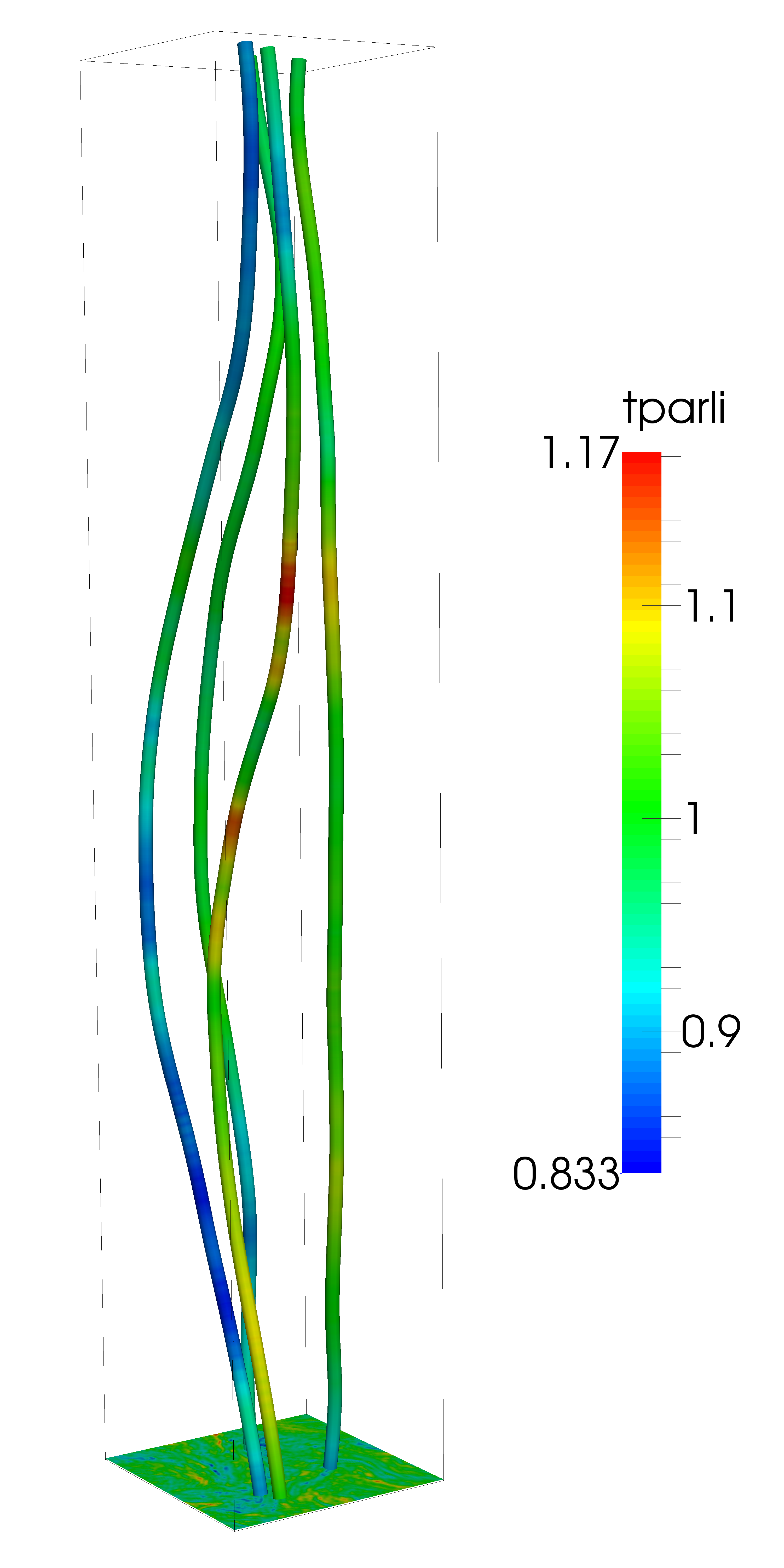
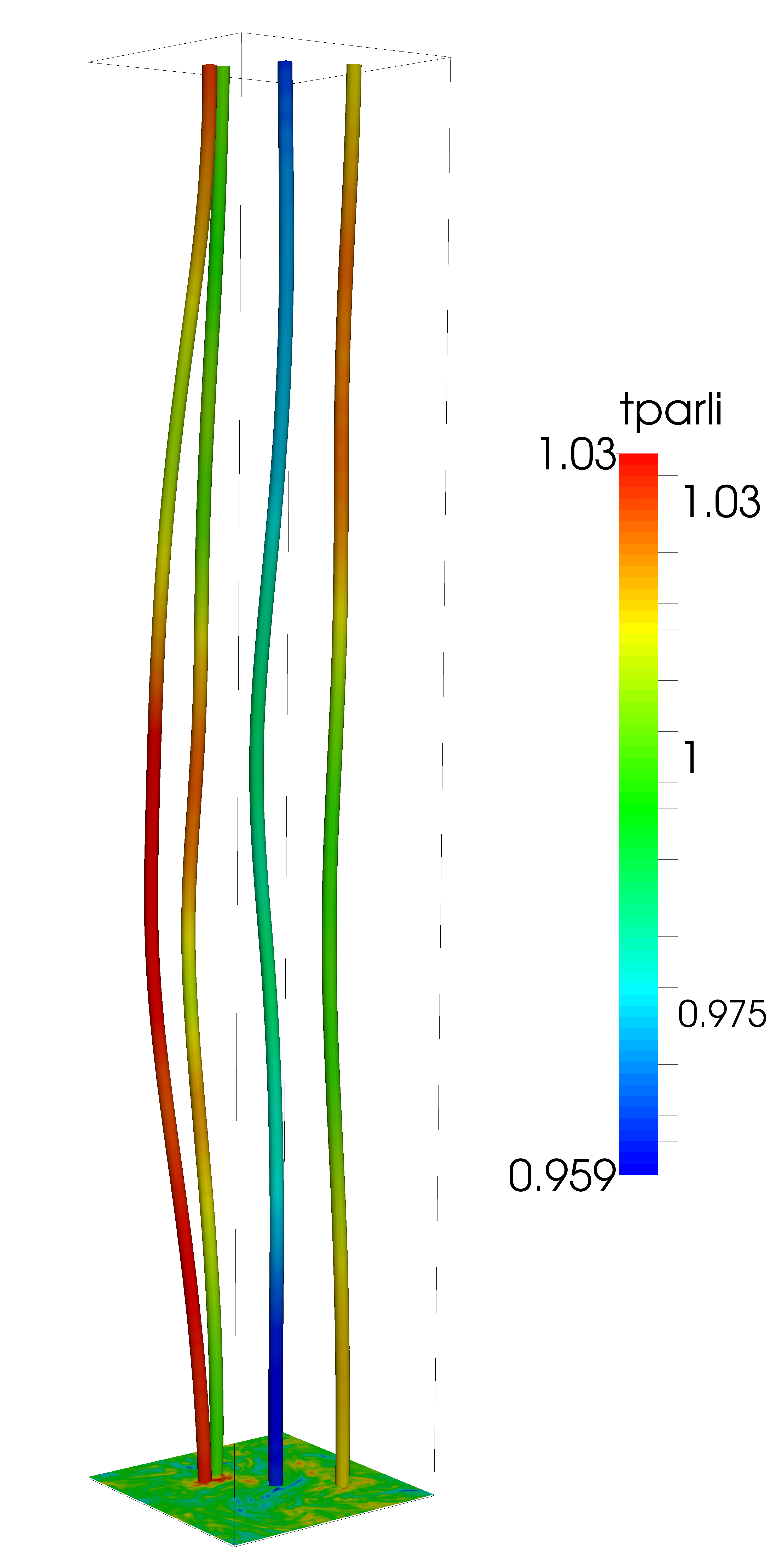
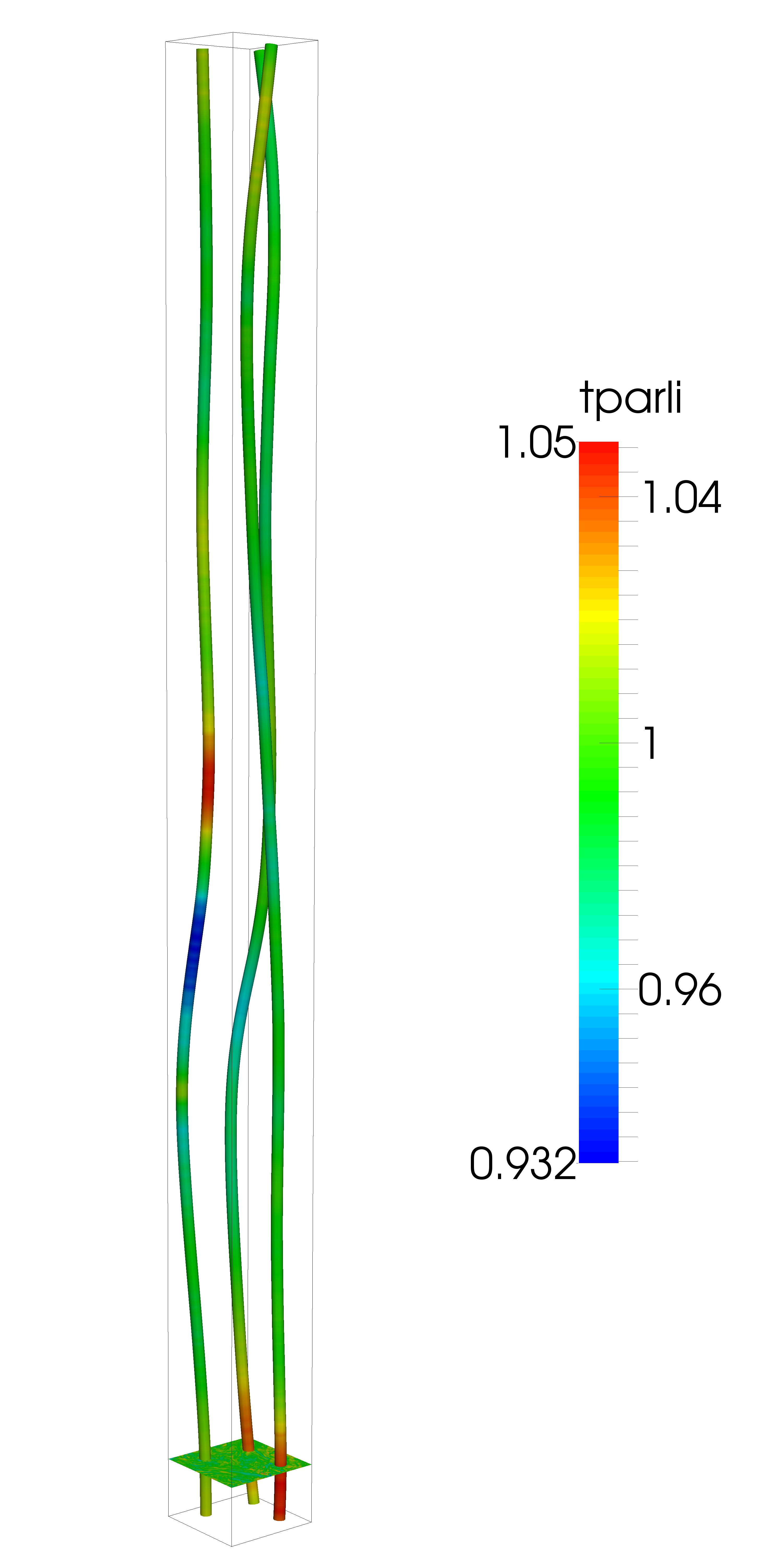
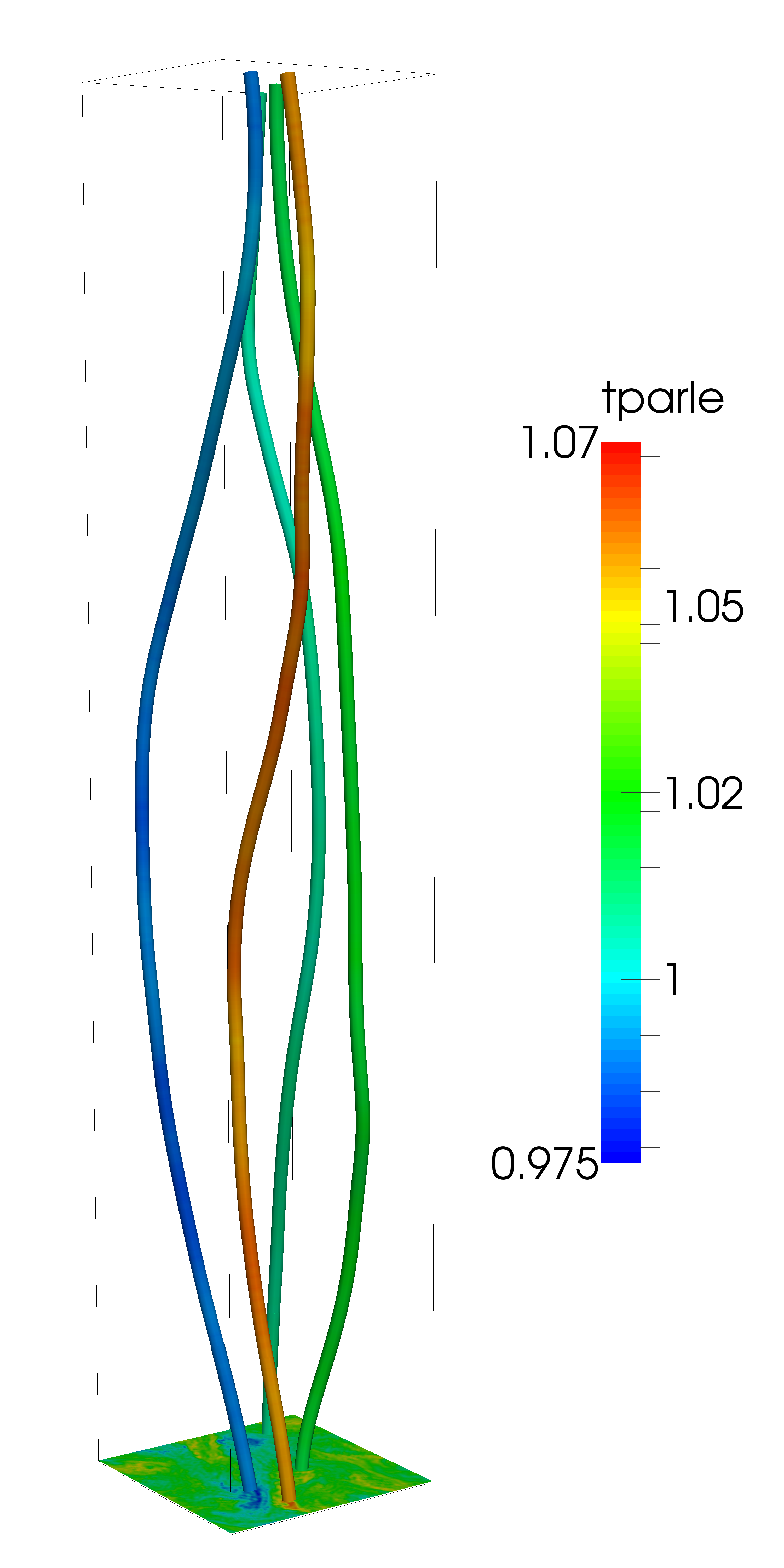
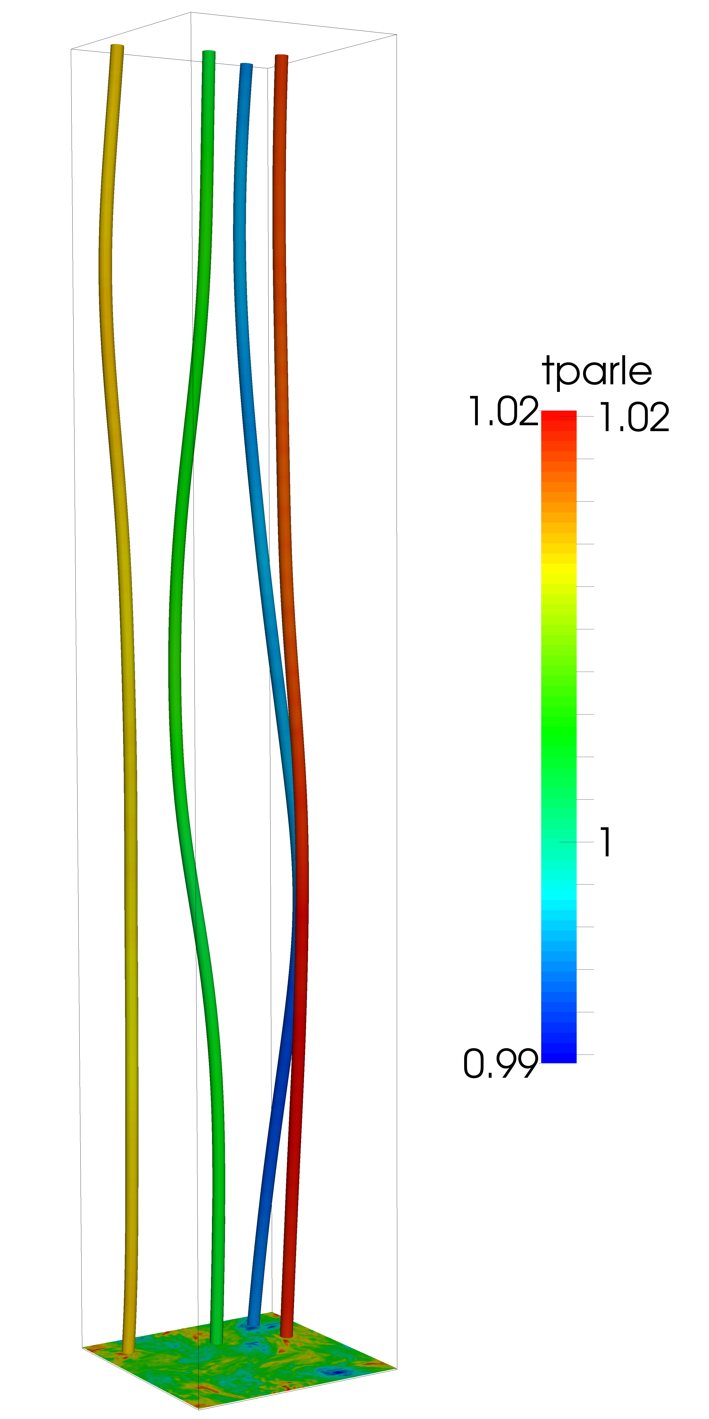
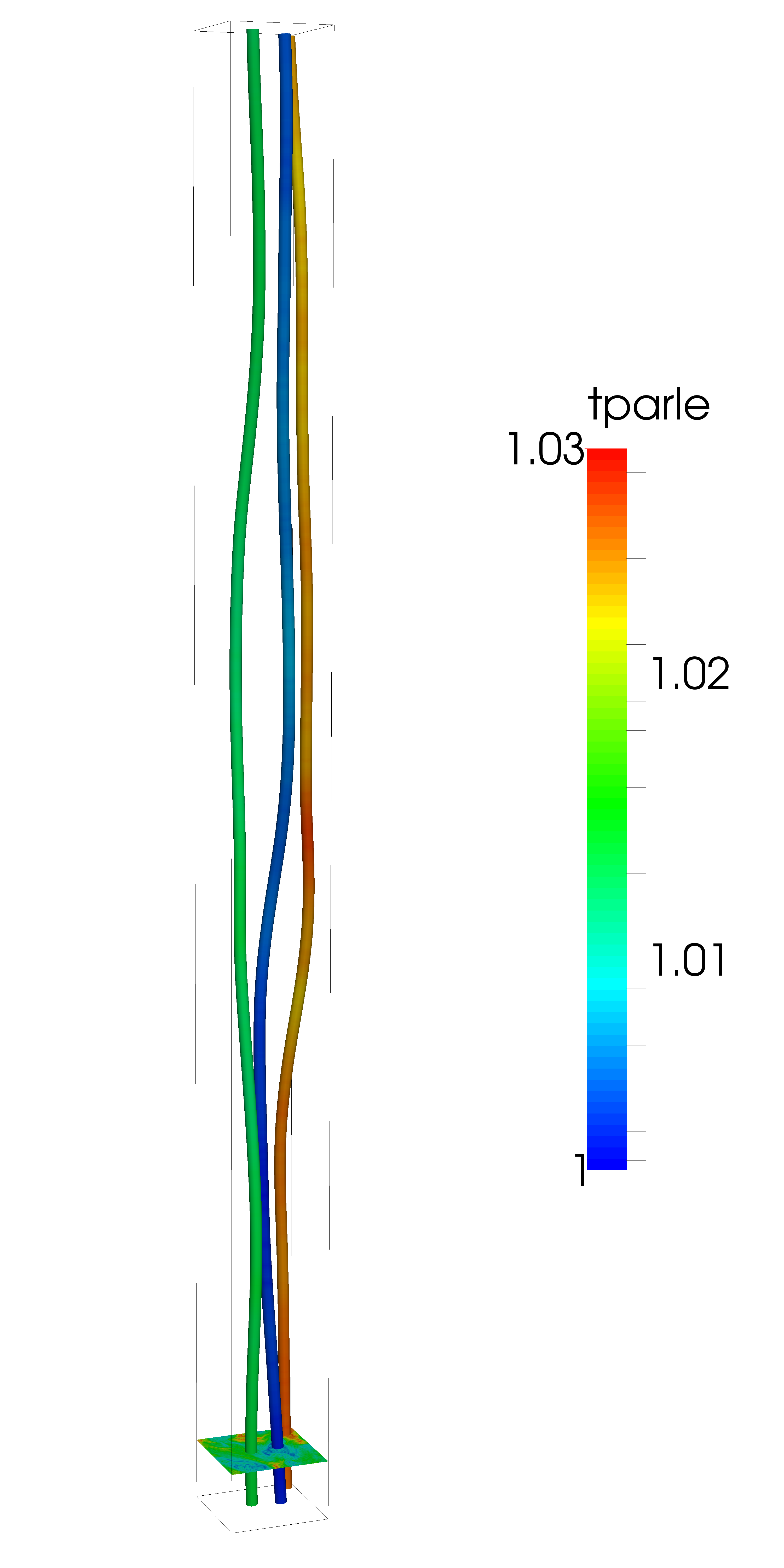
Figure 4: Magnetic field lines colored in function of the parallel temperature of the ions (top) and of the electrons (bottom) for the runs $R_{0.2}^{80}$ (left), $R_{0.08}^{80}$ (middle) and $R_{0.08}^{86}$ (right), when turbulence has reached a stationary state. Different field lines are displayed for the ions and the electrons in order to make more visible the variations of the electron temperature from one line to the other.

Run	$R_{0.2}^{80}$		$R_{0.08}^{80}$		$R_{0.08}^{86}$
$T_{\|i}$	$\sigma_{s}^{2}=1.5\times 10^{-3}$	$L_{s}=13.0$	$\sigma_{s}^{2}=5\times 10^{-5}$	$L_{s}=22.4$	$\sigma_{s}^{2}=1.4\times 10^{-4}$	$L_{s}=34.2$
	$\sigma_{z}^{2}=2.2\times 10^{-3}$	$L_{z}=10.1$	$\sigma_{z}^{2}=8\times 10^{-5}$	$L_{z}=15.9$	$\sigma_{z}^{2}=1.5\times 10^{-4}$	$L_{z}=12.3$
$T_{\|e}$	$\sigma_{s}^{2}=2.2\times 10^{-5}$	$L_{s}=23.6$	$\sigma_{s}^{2}=1.1\times 10^{-6}$	$L_{s}=22.7$	$\sigma_{s}^{2}=1.3\times 10^{-6}$	$L_{s}=53.5$
	$\sigma_{z}^{2}=1.8\times 10^{-4}$	$L_{z}=16.5$	$\sigma_{z}^{2}=9.0\times 10^{-6}$	$L_{z}=16.0$	$\sigma_{z}^{2}=1.3\times 10^{-5}$	$L_{z}=44.6$
$T_{\perp i}$	$\sigma_{s}^{2}=2.2\times 10^{-3}$	$L_{s}=17.2$	$\sigma_{s}^{2}=2.2\times 10^{-4}$	$L_{s}=26.5$	$\sigma_{s}^{2}=2.7\times 10^{-4}$	$L_{s}=42.0$
	$\sigma_{z}^{2}=2.3\times 10^{-3}$	$L_{z}=13.9$	$\sigma_{z}^{2}=2.3\times 10^{-4}$	$L_{z}=19.8$	$\sigma_{z}^{2}=2.6\times 10^{-4}$	$L_{z}=25.0$
$T_{\perp e}$	$\sigma_{s}^{2}=2.2\times 10^{-5}$	$L_{s}=24.3$	$\sigma_{s}^{2}=1.7\times 10^{-6}$	$L_{s}=28.0$	$\sigma_{s}^{2}=3.2\times 10^{-5}$	$L_{s}=67.7$
	$\sigma_{z}^{2}=5.9\times 10^{-5}$	$L_{z}=18.5$	$\sigma_{z}^{2}=6.4\times 10^{-6}$	$L_{z}=16.7$	$\sigma_{z}^{2}=4.4\times 10^{-5}$	$L_{z}=70.0$
$|B|^{2}$	$\sigma_{s}^{2}=7.8\times 10^{-3}$	$L_{s}=16.2$	$\sigma_{s}^{2}=8.9\times 10^{-4}$	$L_{s}=25.1$	$\sigma_{s}^{2}=1.1\times 10^{-3}$	$L_{s}=46.3$
	$\sigma_{z}^{2}=9.4\times 10^{-3}$	$L_{z}=9.2$	$\sigma_{z}^{2}=8.2\times 10^{-4}$	$L_{z}=17.2$	$\sigma_{z}^{2}=1.1\times 10^{-3}$	$L_{z}=24.5$
$|B_{\perp}|^{2}$	$\sigma_{s}^{2}=1.8\times 10^{-3}$	$L_{s}=14.3$	$\sigma_{s}^{2}=2.7\times 10^{-5}$	$L_{s}=15.0$	$\sigma_{s}^{2}=5.9\times 10^{-5}$	$L_{s}=34.0$
	$\sigma_{z}^{2}=2.8\times 10^{-3}$	$L_{z}=14.1$	$\sigma_{z}^{2}=2.4\times 10^{-5}$	$L_{z}=15.3$	$\sigma_{z}^{2}=5.0\times 10^{-5}$	$L_{z}=36.9$

Table 2: Variance of the ion and electron parallel temperatures along magnetic field lines ($\sigma_{s}^{2}$) and along parallels to the $z$-axis ($\sigma_{z}^{2}$), together with the corresponding correlation lengths $L_{s}$ and $L_{z}$ for runs $R_{0.2}^{80}$, $R_{0.08}^{80}$ and $R_{0.08}^{86}$.

A main feature of the phenomenological model discussed in Section 6 concerns the role played by the homogenization of quantities like temperatures along the magnetic field lines, through an effect of particle streaming. The aim of this section is to get some insight into this process. One may expect that it is more efficient for the electrons than for the ions, because of the mass ratio. The question also arises of the influence of the amplitude of the turbulence fluctuations. This issue is qualitatively exemplified in Fig. 4 which displays a few magnetic field lines colored according to the parallel temperature of the ions (top) and of the electrons (bottom) for the runs $R_{0.2}^{80}$ (left), $R_{0.08}^{80}$ (middle) and $R_{0.08}^{86}$ (right). We indeed observe that the parallel electron temperature is significantly more uniform than the parallel ion temperature and that the homogenization process is more efficient for run $R_{0.2}^{80}$ than for run $R_{0.08}^{80}$ corresponding to a smaller nonlinearity parameter. The significant inhomogenity of the ion temperature along the magnetic field lines of run $R_{0.08}^{86}$ demonstrates that $\chi$ rather than the level of the turbulence fluctuations prescribes the dynamics.

These observations can be made more quantitative by computing the variances $\sigma^{2}_{S}$ and $\sigma^{2}_{z}$ and the correlation lengths $L_{s}$ and $L_{z}$ of the ion and electron parallel and perpendicular temperatures, averaged over the 32 field lines mentioned in Section 3.1 (subscript $s$) and over the corresponding lines parallel to the z-axis (subscript $z$). Table 2 collects data concerning run $R_{0.2}^{80}$, $R_{0.08}^{80}$ and $R_{0.08}^{80}$. For comparison, variances and correlation lengths are also presented for the magnetic field amplitude $|B|$ and the transverse component $|B_{\perp}|^{2}$.

Table 2 clearly shows that temperature fluctuations as measured by their respective variances are more important for the ions than for the electrons, and decrease with the amplitude of the magnetic fluctuations, even for comparable values of the nonlinearity parameter $\chi$. The temperature variances along field lines are usually smaller than along the z-direction, except for the perpendicular ion temperature which is less sensitive to Landau damping.

For each run and each particle species, the temperature correlation lengths $L_{s}$ and $L_{z}$ are defined as the integral up to the first zero of the normalized correlation function $\langle T_{\|}({\mathbf{x}^{\prime}}+{\mathbf{x})}T_{\|}({\mathbf{x}^{\prime}})\rangle/\langle T_{\|}({\mathbf{x}})^{2}\rangle$ computed along each of the 32 selected lines and averaged over them. When considering the ideal case of a sinusoidal fluctuation of wavenumber $k=1$, this definition leads to a correlation length equal to one. A correlation $L_{s}$ along the magnetic field lines will thus correspond to a parallel wavenumber $K_{\|}=1/L_{s}$. Similar definitions are given in the case of the fields $|B|^{2}$ and $|B_{\perp}|^{2}$. It is of interest to compare the quantity $K_{\|}$ evaluated for $|B|^{2}$, with the scale-dependent parallel wavenumber $k_{\|}$ previously discussed. From Table 2, the values $K_{\|}$ corresponding to runs $R_{0.2}^{80}$, $R_{0.08}^{80}$ and $R_{0.08}^{86}$ are $0.06$, $0.04$ and $0.02$ respectively, which from Fig. 1 roughly corresponds to values of $k_{\|}$ between $k_{\perp}=0.4$ and $0.6$, a range where the transverse magnetic spectrum starts displaying a power law (Fig. 2, bottom). The correlation length of $|B|^{2}$ in the z-direction is significantly smaller than along the field lines, in contrast with the variances which are of the same order of magnitude. This variation is due to the $B_{z}$ component, as for $|B_{\perp}|^{2}$ both variances and correlations lengths are similar in both directions. The correlation lengths of $|B_{\perp}|^{2}$ are indeed prescribed by the KAW wavelength, and are thus essentially independent of the amplitude of the turbulent fluctuations. When comparing the correlations length for runs $R_{0.2}^{80}$ and $R_{0.08}^{86}$, one recovers the $2.5$ geometric scaling factor between the longitudinal extensions of the computational domains, which is also the ratio of the respective parallel wavelengths of the driven waves.

Considering electron temperatures, the correlation lengths along the field lines are roughly the same for the three runs, up to the $2.5$ scaling factor for $R_{0.08}^{86}$. They are significantly larger than in the z-direction, indicating that Landau damping leads to homogenization along the field lines, but not to isothermal electrons in the full domain. Concerning the ion temperatures, the two runs with the same nonlinearity parameter have similar correlation lengths up to the geometric factor (larger along the field lines than in the z-direction). In contrast, for the run with a smaller value of $\chi$, the correlation lengths are larger.

To summarize, these results show that Landau damping, as implemented in the FLR-Landau fluid code, induces a homogenization of temperature fluctuations along the field lines. They also comfort the assumption of the phenomenological model that the electron homogenization time scale can be ignored, as this process appears to be essentially independent of the turbulence characteristics. The ion temperature correlation length normalized by the parallel wavelength of the driven waves is sensitive to the nonlinearity parameter, suggesting that the nonlinear dynamics is indeed coupled to the ion homogenization process. The influence of this effect on the energy transfer is permitted by the fact that the frequencies $\omega_{H}\sim v_{th}k_{\|}$ and $\omega_{NL}=k_{\perp}v_{e}\sim[k_{\perp}^{5}E_{k}]^{1/2}$ are of the same order of magnitude near the ion gyroscale. Using the fact that $v_{th}\sim v_{A}\sim 1$, we indeed check that, for run $R_{0.2}^{80}$, the ratio $\omega_{NL}/\omega_{H}$ is $0.34$ at $k_{\perp}=1.1$, $0.55$ for $k_{\perp}=2$ and $0.9$ for $k_{\perp}=2.9$, while for run $R_{0.08}^{80}$ this ratio takes the values $0.19$, $0.25$ and $0.34$ for the corresponding values of $k_{\perp}$. This indicates that Landau damping is more efficient in the latter run which displays the steeper spectrum. For comparison, in the case of run $R_{0.08}^{86}$, this ratio takes the values $0.33$, $0.56$ and $0.84$, rather similar to those of run $R_{0.2}^{80}$ that is characterized by the same nonlinearity parameter.

8 Conclusion

The three-dimensional FLR-Landau fluid simulations of sub-ion turbulence in the solar wind analyzed in this paper show a non-universal power-law spectrum for the transverse magnetic energy, with an exponent depending on the nonlinearity parameter, a quantity which is varied by changing the propagation angle and the relative amplitude of the driven KAWs. The nonlinearity parameter, rather than the amplitude of the magnetic fluctuations, prescribes the turbulence strength, governing for example the meandering of the magnetic field lines. The simulation results are supported by a phenomenological model where the departure from the usually predicted $k_{\perp}^{-7/3}$ spectrum originates from the sensitivity of the transfer time to the particle streaming along the magnetic field lines induced by Landau damping. Interestingly, similar simulations where Landau resonance is eliminated by prescribing zero heat fluxes (bi-adiabatic approximation) leads to a $-7/3$ exponent, whatever the value of the nonlinearity parameter. Details will be given elsewhere.

The FLR-Landau fluid simulations also clearly point out the importance of the dynamics along the field lines and in particular the anisotropic homogenization process, which contrasts with the often used assumption of isothermal electrons.

The present simulations, together with the phenomenological modeling, provide an interpretation of the significant dispersion of the sub-ion spectral exponent measured in the solar wind. An interesting development would be to evaluate the nonlinearity parameter from satellite data. This turns out to be a difficult but important issue, especially because correlation of the spectral exponent with the sole amplitude of the turbulence fluctuations in various regions of the solar wind leads to different conclusions.

Although the present simulations seem sufficient to characterize the energy spectrum of the transverse magnetic fluctuations at the sub-ion scales, higher resolutions are in project to capture part of the MHD range and also to increase the extension of the simulated sub-ion spectral domain. The latter development is important to reach scales where the electron-MHD approximation starts to apply.

Appendix A Estimate of the characteristic energy transfer time

Writing the Navier-Stokes equation, or any quadratically nonlinear initial value problem, (neglecting for the sake of simplicity driving and dissipation) in the symbolic form $\partial_{t}u=uu$ and taking the statistical moments, we are led to write (assuming spatial homogeneity)

$$\partial_{t}\langle uu\rangle=\langle uuu\rangle$$ (A1)

$$\partial_{t}\langle uuu\rangle=\langle uuuu\rangle\equiv\langle uu\rangle\langle uu\rangle+\langle uuuu\rangle_{c}$$ (A2)

where we separate the Gaussian contribution symbolically written $\langle uu\rangle\langle uu\rangle$, from the fourth-rank cumulant $\langle uuuu\rangle_{c}$. Neglecting this latter contribution would correspond to the quasi-normal approximation, where the unlimited growth of the third-rank correlations leads to unphysical effects such as negative energy spectra (Ogura, 1963; O’Brien & Francis, 1962; Orszag, 1976). The fourth-order cumulant, providing a coupling with the higher moments of the fluid hierarchy, actually ensures saturation of these correlations. By an argument similar to that used to introduce the concept of turbulent viscosity, we write $\langle uuuu\rangle_{c}=-\eta\langle uuu\rangle$. After a transient, we thus get a quasi-equilibrium state where $\langle uuu\rangle=\eta^{-1}\langle uu\rangle\langle uu\rangle$, which is substituted in Eq. (A1) that becomes

$$\partial_{t}\langle uu\rangle=\eta^{-1}\langle uu\rangle\langle uu\rangle.$$ (A3)

This equation is in fact an integrodifferential equations involving wavevector triads. Here, we will drastically simplify this model by assuming strict locality of the interactions. When turning to the energy spectrum, we are then led to write

$$\partial_{t}E_{k}=\eta^{-1}\omega_{NL}^{2}E_{k},$$ (A4)

on a dimensional basis, noting that only energy spectrum and wavenumber are entering the equation. We can then define an energy transfer time $\tau_{tr}=\omega_{tr}^{-1}$ with $\omega_{tr}=\eta^{-1}\omega_{NL}^{2}$, where the relaxation rate $\eta$ of triple correlations is estimated as the sum of the frequency of the contributing processes. In purely hydrodynamic turbulence $\eta=\omega_{NL}$, so $\omega_{tr}=\omega_{NL}$. In standard (weak) wave turbulence where $\omega_{W}\gg\omega_{NL}$, we have $\omega_{tr}=\omega_{NL}^{2}/\omega_{W}$. Here, we also have to take into account the contribution of the homogenization process along the field lines of frequency $\omega_{H}$. Note that, except in pure hydrodynamic turbulence, it is not necessary to retain $\omega_{NL}$ in the definition of $\eta$ as it either negligible compared with $\omega_{W}$ when the turbulence is weak or displaying the same $k_{\perp}$ scaling in the case of critical-balanced turbulence. This leads us to write

$$\omega_{tr}=\frac{\omega_{NL}^{2}}{\omega_{W}+\omega_{H}}=\frac{\Lambda^{2}{\overline{\alpha}}^{2}k_{\perp}^{3}E_{k}}{{\overline{\omega}}v_{A}k_{\|}+\mu v_{th}k_{\|}}$$ (A5)

where ${\overline{\alpha}}={\overline{\omega}}\sim k_{\perp}\rho_{i}$, while $\Lambda$ and $\mu$ are numerical constant.

References

- Alexandrova et al. (2013) Alexandrova, O., Chen, C. H. K., Sorriso-Valvo, L., Horbury, T. S., & Bale, S. D. 2013, Space Sci. Rev., 178, 102
- Alexandrova et al. (2008) Alexandrova, O., Lacombe, C., & Mangeney, A. 2008, Ann. Geophys., 26, 3585–3596
- Alexandrova et al. (2012) Alexandrova, O., Lacombe, C., Mangeney, A., Grappin, R., & Maksimovic, M. 2012, Astrophys. J., 760, 121
- Bale et al. (2013) Bale, S. D., Pulupa, M., Salem, C., Chen, C. H. K., & Quataert, E. 2013, J. Astrophys. Lett., 769, L22
- Boldyrev et al. (2013) Boldyrev, S., Horaites, K., Xia, Q., & Perez, J. C. 2013, Astrophys. J, 777, 41
- Boldyrev & Perez (2012) Boldyrev, S., & Perez, J. C. 2012, Astrophys. J. Lett., 758, L44
- Borgogno et al. (2008) Borgogno, D., Grasso, D., Pegoraro, F., & Schep, T. J. 2008, Phys. Plasmas, 15, 102308
- Bratanov et al. (2013) Bratanov, V., Jenko, F., Hatch, D. R., & Wilczek, M. 2013, Phys. Rev. Lett., 111, 075001
- Bruno et al. (2014) Bruno, B., Trenchi, L., & Telloni, D. 2014, J. Astrophys. Lett., 793, L15
- Bruno & Carbone (2013) Bruno, R., & Carbone, V. 2013, Living Rev. Solar Phys., 10
- Chen et al. (2013) Chen, C. H. K., Boldyrev, S., Xia, Q., & Perez, J. C. 2013, Phys. Rev. Lett., 110, 225002
- Cho et al. (2002) Cho, J., Lazarian, A., & Vishniac, E. T. 2002, Astrophys. J. Lett., 566, L49
- Gary et al. (2012) Gary, S. P., Chang, O., & Wang, J. 2012, Astrophys. J., 755, 142
- Goldreich & Shridhar (1995) Goldreich, P., & Shridhar, S. 1995, Astrophys. J., 438, 763
- Hollweg (1974) Hollweg, J. V. 1974, J. Geophys. Res., 29, 3845
- Howes et al. (2006) Howes, G. G., Cowley, S. C., Dorland, W., & Hammett, G. W. 2006, Astrophys. J., 651, 590
- Howes et al. (2008) Howes, G. G., Cowley, S. C., Dorland, W., et al. 2008, J. Geophys. Res., 113, A05105
- Howes et al. (2011a) Howes, G. G., TenBarge, J. M., & Dorland, W. 2011a, Phys. Plasmas, 18, 102305
- Howes et al. (2011b) Howes, G. G., TenBarge, J. M., Dorland, W., et al. 2011b, Phys. Rev. Lett., 107, 035004
- Kanekar et al. (2015) Kanekar, A., Schekochihin, A. A., Dorland, W., & Loureiro, N. F. 2015, J. Plasma Phys., 81, 305810104
- Landi et al. (2014) Landi, S., Matteini, L., & Pantelini, F. 2014, J. Astrophys. Lett., 790, L12
- Latinen et al. (2015) Latinen, T., Kopp, A., Effenberger, F., Dalla, S., & Mash, M. S. 2015, arXiv:1508.03164v1 [astro-ph.SR]
- Lesieur (2008) Lesieur, M. 2008, Turbulence in fluids ( ed.) (Springer)
- Meyrand & Galtier (2013) Meyrand, R., & Galtier, S. 2013, Phys. Rev. Lett., 111, 264501
- Nazarenko & Schekochihin (2011) Nazarenko, S. V., & Schekochihin, A. A. 2011, J. Fluid Mech., 677, 134
- O’Brien & Francis (1962) O’Brien, E. F., & Francis, G. C. 1962, J. Fluid. Mech., 13, 369
- Ogura (1963) Ogura, Y. 1963, J. Fluid. Mech., 16, 33
- Orszag (1970) Orszag, S. A. 1970, J. Fluid Mech., 41, 363
- Orszag (1976) Orszag, S. A. 1976, in Fluid Dynamics 1973, ed. R. Balian & J. L. Peube, Les Houches Summer School of Theoretical Physics (Gordon and Breach), 236–374
- Passot et al. (2014) Passot, T., Henri, P., Laveder, D., & Sulem, P. L. 2014, Euro. Phys. J. D, 68, 207
- Passot & Sulem (2015) Passot, T., & Sulem, P. L. 2015, Astrophys. J. Lett., 812, L37
- Pouquet et al. (1976) Pouquet, A., Frisch, U., & Léorat, J. 1976, J. Fluid Mech., 77, 321
- Sahraoui et al. (2010) Sahraoui, F., Goldstein, M. L., Belmont, G., Canu, P., & Rezeau, L. 2010, Phys. Rev. Lett., 105, 131101
- Sahraoui et al. (2009) Sahraoui, F., Goldstein, M. L., Robert, P., & Khotyaintsev, Y. V. 2009, Phys. Rev. Lett., 102, 231102
- Sahraoui et al. (2013) Sahraoui, F., Huang, S. Y., Belmont, G., et al. 2013, Astrophys. J., 777, 11
- Sahraoui et al. (2011) Sahraoui, F., Goldstein, M. L., Belmont, G., et al. 2011, Planet. Space Sc., 59, 585
- Schekochihin et al. (2015) Schekochihin, A. A., Parker, J. T., Highcock, E. G., et al. 2015, eprint arXiv:1508.05988
- Servidio et al. (2015) Servidio, S., Valentini, F., Perrone, D., et al. 2015, J. Plasma Phys., 81, 325810107
- Smith et al. (2006) Smith, C. W., Hamilton, K., Vasquez, B. J., & Leamon, R. J. 2006, Astrophys. J. Lett., 645, L85
- Snyder et al. (1997) Snyder, P. B., Hammett, G. W., & Dorland, W. 1997, Phys. Plasmas, 4, 3974
- Spitzer & Härm (1953) Spitzer, L., & Härm, R. 1953, Phys. Rev., 89, 977
- Sulem et al. (1975) Sulem, P. L., Lesieur, M., & Frisch, U. 1975, Ann. Geophys., 31
- Sulem & Passot (2015) Sulem, P. L., & Passot, T. 2015, J. Plasma Phys., 81(1), 325810103
- TenBarge et al. (2014) TenBarge, J. M., Howes, G. C., Dorland, W., & Hammett, G. W. 2014, Comp. Phys. Comm., 185, 578
- Told et al. (2015) Told, D., Jenko, F., TenBarge, J. M., Howes, G. G., & Hammett, G. 2015, Phys. Rev. Lett., 115, 025003
- Wan et al. (2015) Wan, M., Matthaeus, W. H., Roytershteyn, V., et al. 2015, Phys. Rev. Lett., 114, 175002