Centripetal focusing of gyrotactic phytoplankton in solid-body rotation

Abstract

A suspension of gyrotactic microalgae Chlamydomonas augustae swimming in a cylindrical water vessel in solid-body rotation is studied. Our experiments show that swimming algae form an aggregate around the axis of rotation, whose intensity increases with the rotation speed. We explain this phenomenon by the centripetal orientation of the swimming direction towards the axis of rotation. This centripetal focusing is contrasted by diffusive fluxes due to stochastic reorientation of the cells. The competition of the two effects lead to a stationary distribution, which we analytically derive from a refined mathematical model of gyrotactic swimmers. The temporal evolution of the cell distribution, obtained via numerical simulations of the stochastic model, is in quantitative agreement with the experimental measurements in the range of parameters explored.

I Introduction

Many phytoplankton species are able to swim and their motility affects several basic processes in their life and ecology Smayda (1997); Reynolds (2006); Kiørboe (2008); Elgeti et al. (2015). Swimming allows phytoplankton to explore the water column, moving from the well-lit surface layers during the day to the nutrients-rich deeper layers at night Lieberman et al. (1994); Cullen (1985) (see also Bollens et al. (2011) and references therein). In order to perform this vertical migration, many phytoplankton cells are guided by an orienting mechanism when swimming. One of the simplest mechanism leading to orientation in the vertical direction is bottom-heaviness Wager (1910). The unbalanced distribution of mass inside the cell induces a mechanical torque, due to gravity and buoyancy forces, which orients the cell in the direction opposite to gravity. This torque competes with the viscous torque, due to the hydrodynamic shear, which tends to rotate the cell. When the swimming direction results from the balance between this two torques, the organism is said to be gyrotactic Kessler (1985); Pedley and Kessler (1987, 1992).

Gyrotaxis generates remarkable spatial distributions of swimming cells. In laminar conditions, it produces beam-like accumulations in vertical pipe flows Kessler (1985) and concentrated thin layers in horizontal shear flows Durham et al. (2009). More recently, it has been shown by theoretical analysis and numerical simulations, that gyrotaxis induces intense small-scale fractal clustering in turbulent flows Durham et al. (2013); Zhan et al. (2014); Fouxon and Leshansky (2015); Gustavsson et al. (2015), providing a mechanisms for the micro-patchiness observed in motile phytoplankton Malkiel et al. (1999). Turbulence is characterized by extreme fluctuations of fluid acceleration, which can locally exceed gravity even at moderate Reynolds numbers La Porta et al. (2001). The origin of these fluctuations has been traced back to small-scale vortices generating intense centripetal accelerations Biferale et al. (2005). For applications in turbulent flow, the gyrotactic model has been recently modified to take into account the effect of fluid acceleration in the mechanical torque De Lillo et al. (2013). Remarkably, numerical simulations of turbulent flows have shown that the effect of fluid acceleration is to enhance the patchiness of gyrotactic phytoplankton by gathering cells into small-scale vortices De Lillo et al. (2014).

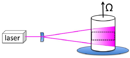
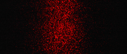
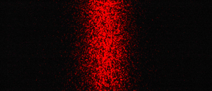
Figure 1: Online version in colour. Sketch of the experimental setup. The cylindrical vessel filled with a suspension of C. augustae is placed over a table rotating with angular velocity $\Omega=2\pi f$. A blue laser (power $100\,mW$, wavelength $\lambda=450\,nm$) vertical sheet, generated by a cylindrical lens, is directed in the central plane of the vessel. Fluorescent images of cells are acquired by a Nikon CCD camera at resolution $3000\times 2000$ pixels with a low-pass red filter at $600\,nm$. The rectangular area represents the measurement region. The pictures on the right are two examples of the images (central part) taken by the camera at the time $t=600\,s$ for $f=5\,Hz$ (top) and $f=8\,Hz$ (bottom).

In this work, we study experimentally, analytically and numerically the behavior of gyrotactic swimming cells in a controlled environment of uniform vorticity – i.e. a cylindrical water vessel in solid-body rotation. Preliminary, qualitative, results of the experiment were described in Ref De Lillo et al. (2014). We show that phytoplankton cells, initially uniformly distributed in the container, aggregate towards the axis of rotation eventually reaching a stationary, Gaussian-like distribution. We show analytically and by means of numerical simulations that a stochastic formulation of the refined gyrotactic model De Lillo et al. (2014), which takes into account the fluctuations of the swimming direction, is able to reproduce quantitatively the time evolution of a distribution of cells and the asymptotic accumulation at different rotation frequency.

The remaining of the paper is organized as follows. In Section II we introduce the experimental method, the theoretical model, the different analytical techniques and the numerical method. In Section III we discuss the data analysis and we compare the experimental results with the theoretical and numerical predictions. Finally, Section IV is devoted to conclusions. Technical details on the analytical computations are presented in the Appendices.

II Methods

II.1 Laboratory experiments

We performed laboratory experiments using cultures of the unicellular freshwater flagellate strain of Chlorophyceae, Chlamydomonas augustae. C. augustae is inoculated in $250\,ml$ Erlenmeyer flasks containing $200\,ml$ of liquid Z medium Andersen (2005). Cultures are kept at constant temperature of $25^{o}\,C$ under artificial illumination provided by fluorescent light producing about $2000\,lux$ with a $16:8\,h$ light:dark cycle. Culture growth is estimated by measuring the dry biomass concentration and the number of cells. Samples for dry weight ($dw$) calculation are taken in triplicate and a gravimetric determination is performed Chini Zittelli et al. (2000). Triplicate cell counts are carried out for each sample by loading $0.01\,ml$ of sample on a Thoma’s counting chamber and the averaged value was determined. Cell counts are performed by using a hemocytometer. Experiments are realized about $3$ weeks after inoculation of the culture and after dilution into fresh medium to reach a concentration of $\simeq 5\times 10^{4}\,cell/ml$ to avoid collective phenomena.

The experimental setup is sketched in Fig. 1. A suspension of gyrotactic cells is placed in a small cylindrical vessel of inner radius $R=18\,mm$ and height $H=57\,mm$ over a plate that rotates at angular velocity $\Omega$, digitally controlled. After a short spin-up time of order $R/(\nu\Omega)^{1/2}$ ($\nu$ is the kinematic viscosity of water) the fluid in the vessel reaches the solid-body rotation regime Greenspan and Howard (1963), at which we defines the reference zero time for the experiment. We remark that this regime is reached after a series of physical processes characterized by complex secondary flows. Nonetheless, this initial transient is negligible since the spin-up time for our vessel is of the order of few seconds and the displacement of the swimming cells in this transient is very small.

All these preparatory processes are performed in darkness or with a low power red light at wavelength $655\,nm$ not seen by algae Harris (2009). At time $t=0$ and every $\Delta t$ (typically $\Delta t=15\,s$) a blue laser sheet (power $100\,mW$, wavelength $\lambda=450\,nm$) from one side of the vessel is turned on for less than one second and a picture of the vessel is taken by the camera and acquired by the computer. Each experiment, for a specific value of $\Omega$, lasts for $15$ minutes after which the plate is stopped and the culture is homogenized. Control experiments are performed in similar conditions by using a suspension of cells killed with a solution of $8\%$ v/v ethanol. The frequency of rotation $f=\Omega/(2\pi)$ ranges between $4\,Hz$ and $8\,Hz$, corresponding to a centripetal acceleration $a_{c}=\Omega^{2}R$ at the border of the vessel between $11\,m/s^{2}$ and $45\,m/s^{2}$, in all cases larger than the gravitational acceleration.

The laser sheet induces fluorescence of the C. augustae cells whose emission spectrum has a peak around $685\,nm$ (determined by a spectrophotometer) Harris (2009). Fluorescence images are taken by a digital camera (resolution $3000\times 2000$ pixels) with a red filter (B+W $091$ Dark Red) which cuts all wavelengths below $600\,nm$. Samples of the fluorescence images are shown in Fig. 1. Calibration of the images with the cell density is performed by taking pictures of homogeneous suspension (not in rotation) with known concentrations (determined by a hemocytometer). Images of the vessel filled with distilled water are used to define the background noise (due to background light and CCD noise) which is averaged over realizations and space and removed from the experimental images. Spatial calibration is performed by a micrometric pattern inside the vessel filled with water, which is also used to compensate the optical deformation induced by the cylindrical surface of the vessel.

Images acquired by the camera at different times are used to measure the evolution of the radial density $n_{exp}(r,t)$ of algae, after averaging over the vertical direction (we do not observe significant dependence of the local density on the vertical coordinate). The radial density is computed over a portion of the image of height $h=30$ mm and width $2R_{v}=24$ mm centered at the cylinder axis. We limit the acquisition to $R_{v}<R$ in order to reduce optical deformations and possible wall effects.

II.2 Mathematical models

The mathematical model for gyrotactic algae was introduced by Kessler and Pedley Kessler (1985); Pedley and Kessler (1987, 1990), on the basis of the observation that bottom-heavy swimming micro-organisms focus in the center of a pipe when the fluid flows downwards. The swimming direction results from the competition between gravity-buoyant torque, due to bottom-heaviness, and the shear-induced viscous torque. Recently, the model has been extended to include the acceleration induced by the fluid flow De Lillo et al. (2013, 2014), an effect which can be important in turbulence La Porta et al. (2001).

Due to the small size ($\sim 10\mu m$) and the small density mismatch with the fluid (less than $5\%$), cells are represented as point-like, spherical and neutrally buoyant particles (for a recent refined analysis see Ref. O’Malley and Bees (2012)) transported by the fluid velocity ${\bm{u}}({\bm{x}},t)$ at cell position $\bm{x}$ with a superimposed swimming velocity ${\bm{v}}_{s}$

$$\dot{\bm{x}}={\bm{u}}+v_{s}{\bf p}\,.$$ (1)

The magnitude of the swimming velocity, $v_{s}$, is assumed constant, while the swimming direction ${\bf p}$ evolves as

$$\dot{\bf p}=-\frac{1}{2v_{o}}\left[\bm{A}-(\bm{A}\cdot{\bf p}){\bf p}\right]+\frac{1}{2}{\bm{\omega}}\times{\bf p}+{\bf\Gamma_{\mathrm{r}}}\,.$$ (2)

The first term describes the orientation towards the direction opposite to the acceleration $\bm{A}$ in the cell reference of frame with characteristic speed $v_{o}=3\nu/\delta$ ($\delta$ is the cell center-of-mass displacement relative to the geometrical center and $\nu$ the fluid kinematic viscosity). In the original model only gravity is taken into account and ${\bm{A}}={\bm{g}}$. Here, following De Lillo et al. (2013, 2014), we consider the total acceleration, due to gravity and fluid acceleration ${\bm{a}}=d{\bm{u}}/dt$ (acceleration due to swimming is neglected), so that $\bm{A}=\bm{g}-\bm{a}$. The second term in the rhs of (2) represents cell rotation due to the local vorticity ${\bm{\omega}}={\bm{\nabla}}\times{\bm{u}}$. The last term $\bm{\Gamma}_{\mathrm{r}}$ represents rotational diffusion in the swimming directions, which phenomenologically models the intrinsic stochasticity in the swimming behavior Hill and Häder (1997).

We emphasize the simplicity of the above model that neglects many details, including the unsteadiness of swimming due to flagella beating, deviations from spherical shape, cell-cell interactions and the feedback of cell motion on the surrounding fluid.

II.3 Deterministic motion in solid body rotation

We study analytically and numerically the motion of gyrotactic swimmers in the velocity field generated by the solid body rotation of the cylinder along its vertical axis: ${\bm{u}}=(-\Omega y,\Omega x,0)$. Vorticity is parallel to gravity, ${\bm{\omega}}={\bm{\nabla}}\times{\bm{u}}=(0,0,2\Omega)$, and the (centripetal) acceleration ${\bm{a}}=(-\Omega^{2}x,-\Omega^{2}y,0)$ is orthogonal to gravity ${\bm{g}}=(0,0,-g)$.

We start by considering the dynamics in the absence of stochastic terms (i.e. $\bm{\Gamma}_{\mathrm{r}}=0$ in (2)) whose effects will be discussed in the following Section. In this limit it is possible to derive analytically the motion of swimming cells and show that they accumulate exponentially in time on the axis of rotation.

By introducing cylindrical coordinates with ${\bf x}=({\bf r},z)$ and ${\bf p}=({\bf p}_{r},p_{z})$, such that $\bm{A}=(\Omega^{2}\bm{r},-g)$ and $\bm{u}=(\Omega\bm{r}^{\perp},0)$ (with ${\bm{r}}^{\perp}=(-y,x)$), Eqs. (1-2) become

$$\dot{\bf r} = \Omega{\bf r}^{\perp}+v_{s}{\bf p}_{r}$$ (3)

$$\dot{z} = v_{s}p_{z}$$ (4)

$$\dot{\bf p}_{r} = -\frac{1}{2B}\left[\gamma{\bf r}+p_{z}{\bf p}_{r}-\gamma({\bf r}\cdot{\bf p}_{r}){\bf p}_{r}\right]+\Omega{\bf p}_{r}^{\perp}$$ (5)

$$\dot{p}_{z} = \frac{1}{2B}\left[1-p_{z}^{2}+\gamma({\bf r}\cdot{\bf p}_{r})p_{z}\right]$$ (6)

where ${\bf p}_{r}^{\perp}=(-p_{y},p_{x})$. The two parameters $B\equiv v_{o}/g$ and $1/\gamma\equiv g/\Omega^{2}$ represents the characteristic time of reorientation under gravity and the radial distance at which fluid and gravitational acceleration are equal.

A solution of the above equations can be obtained under the hypothesis of local equilibrium in the swimming direction, i.e. by assuming $\dot{\bf p}=0$ locally. Physically this requires that the characteristic orientation time $B$ is faster than the typical displacement time. Within this approximation one can show (see Appendix A) that the equilibrium swimming direction ${\bf p}^{eq}$ is simply opposite to the total acceleration, $-\bm{A}$, i.e.

$${\bf p}^{eq}=\frac{\bm{a}\!-\!\bm{g}}{|(\bm{a}\!-\!\bm{g})|}=\left(\frac{-\gamma\bm{r}}{\sqrt{1+(\gamma r)^{2}}},\frac{1}{\sqrt{1+(\gamma r)^{2}}}\right)\,.$$ (7)

When $\gamma r\ll 1$, the distance from the axis evolves as $\dot{r}=-\gamma v_{s}r$ implying that cells position moves exponentially towards the rotation axis $r=0$:

$$r(t)=r(0)e^{-\gamma v_{s}t}\,.$$ (8)

For general values of $\gamma r$ the time evolution of $r(t)$ is more complicated but asymptotically the above results remain valid (see Appendix A for details).

II.4 Stationary distribution in presence of rotational diffusivity

The deterministic model predicts that swimming cells should converge on the rotation axis. In reality, stochastic reorientation of the swimming direction, due to different biological behaviors, causes the cells to weakly deviate from the convergent trajectories predicted by (8), preventing the population from collapsing onto the rotation axis and eventually producing accumulation in a finite volume.

Because we are considering stochastic effects, which can be conveniently modeled as rotational diffusivity Hill and Häder (1997); Pedley and Kessler (1992), in the following we will not discuss individual trajectories, rather we shall focus on the cell density $n(\bm{x},t)$ which can be directly compared with the experimental measurements. We report here the basic ingredients and results of our approach, which is based on the so-called Generalized Taylor Dispersion theory Frankel and Brenner (1989), applied to gyrotactic phytoplankton Bearon et al. (2011, 2012). The interested reader can find details of this approach in Refs. Hill and Bees (2002); Manela and Frankel (2003); Bearon et al. (2011, 2012) (see also Appendix B).

We introduce the probability density function $\mathcal{P}({\bm{x}},{\bf p},t)$ to find a cell at position ${\bf x}$ swimming in direction ${\bf p}$. The evolution of $\mathcal{P}$ is ruled by the Fokker-Planck equation

$$\partial_{t}\mathcal{P}+{\bm{\nabla}}_{\bm{x}}\cdot(\dot{\bm{x}}\mathcal{P})+{\bm{\nabla}}_{\bf p}\cdot(\dot{\bf p}\mathcal{P}-d_{\mathrm{r}}{\bm{\nabla}}_{\bf p}\mathcal{P})=0\,,$$ (9)

where $\dot{\bm{x}}$ and $\dot{\bf p}$ are given by (1) and (2) and $d_{\mathrm{r}}$ is the rotational diffusivity coefficient Pedley and Kessler (1990, 1992). The quantity we are interested in is the population density, $n(\bm{x},t)=\int\mathrm{d}{\bf p}\,\mathcal{P}({\bm{x}},{\bf p},t)$. Essentially, we seek for an effective evolution equation for the population density in terms of the advection-diffusion equation Pedley and Kessler (1990, 1992); Bees et al. (1998); Hill and Bees (2002); Manela and Frankel (2003); Bearon et al. (2011, 2012)

$$\partial_{t}n+{\bm{\nabla}}_{\bm{x}}\cdot(\bm{V}n-\mathbb{D}\bm{\nabla}_{\bm{x}}n)=0\,,$$ (10)

where $\bm{V}$ and $\mathbb{D}$ are the effective drift and diffusivity tensor, respectively.

Leaving the details in the Appendix B, the main idea for going from (9) to (10) is to assume that the orientation dynamics is the fastest process. Consequently, we can treat ${\bf p}$ as a random unit vector with probability density function $f({\bf p})$ given by the stationary solution of the Fokker-Planck equation $\partial_{t}f+\bm{\nabla}_{\bf p}\cdot(\dot{{\bf p}}f-d_{\mathrm{r}}\nabla_{\bf p}f)=0$ Pedley and Kessler (1990, 1992); Bees et al. (1998). Within this approximation the effective drift becomes $\bm{V}=\bm{u}+v_{s}\langle{\bf p}\rangle=\bm{u}+v_{s}\int\mathrm{d}{\bf p}\,{\bf p}f({\bf p})$. The derivation of the diffusivity tensor is more complicated. The Generalized Taylor dispersion has been used to derive $\mathbb{D}$ in homogeneous shear flow Hill and Bees (2002); Manela and Frankel (2003). The method can be extended to inhomogeneous shears provided that the relaxation in the swimming direction is sufficiently fast Bearon et al. (2011). We are here in a similar situation: the equilibrium orientation direction depends on the distance from the axis, according to (7). We therefore assume that, at each distance $r$, the distribution of orientations relaxes to a stationary distribution which parametrically depends on $r$. Within this adiabatic approximation, we are able to obtain explicit expressions for the drift coefficient and the diffusivity tensor.

Once ${\bf V}(r)$ and $\mathbb{D}(r)$ are known, we can solve (10) at stationarity, i.e. when centripetal flux, controlled by swimming, is balanced by the diffusive (centrifugal) flux due to random reorientation. The main analytical result of our analysis is the explicit expression of the stationary radial population density which, for $(\gamma r)\ll 1$, takes the Gaussian form (see Appendix B for details)

$$n_{s}(r)=\mathcal{N}\exp\left(-\frac{\gamma r^{2}}{2v_{s}BF_{3}^{2}(\lambda)}\right)$$ (11)

where $F_{3}(\lambda)$ a dimensionless function of the parameter $\lambda=1/(2Bd_{r})$, and the coefficient $\mathcal{N}$ can be written in terms of the total number of cells $N_{s}$ as $\mathcal{N}=N_{s}\gamma/(2\pi Hv_{s}BF_{3}^{2}(\lambda))$.

From the distribution (11) we obtain the average distance of the population from the cylinder axis in stationary conditions which reads

$$\langle r\rangle_{s}\equiv\frac{\int_{0}^{R}rn_{s}(r)dr}{\int_{0}^{R}n_{s}(r)dr}=\sqrt{\frac{2}{\pi}}\left(\frac{v_{s}B}{\gamma}\right)^{1/2}F_{3}(\lambda)\,,$$ (12)

where the subleading contribution from the upper integration extreme $R$ has been neglected.

II.5 Population evolution: numerical simulations

The temporal evolution of the cell density cannot in general be obtained analytically. Therefore, in order to compare the model with the experimental measurements, we performed a Monte Carlo simulations of (9) directly simulating stochastic trajectories from Eqs (3, 5,6) using a Runge-Kutta fourth order scheme (the vertical dynamics (4) is not needed as we are interested in the radial distribution). The cell’s parameters $v_{s}$, $B$ and $d_{r}$ are chosen, among the typical values given in literature, in order to have a good fit of the stationary distribution, as described below. The parameter $\gamma=\Omega^{2}/g$ is varied according to the experimental rotation frequency, with $g=9.8\,m/s^{2}$.

The simulation is initialized placing $N_{s}=10^{5}$ cells randomly in a circle of radius $R=18$mm with random swimming orientations uniformly distributed on the unit sphere. We use a time step of $10^{-3}s$ and store the position and velocities of the cells every $15\,s$, as in the experiment. From the stored position we can reconstruct the cell density and other observable. In particular, we will be interested in the evolution of the average radial distance $\langle r(t)\rangle=\int drn(r,t)r/\int drn(r,t)$.

III Data analysis and results

In this Section we compare the predictions of the mathematical model presented in Methods with the outcome of the experiments. The analytical theory of Sect. II.4 provides an explicit expression for the radial population density $n_{s}(r)$ at equilibrium, while the time evolution of the density is obtained by stochastic simulations of (9).

In order to compare experimental and theoretical data we have to modify the theory of Section II by adding to the theoretical population density $n(r,t)$ a constant population of non-motile cells of uniform density $b$. Indeed a fraction of the cell population does not move (or it moves very slowly) and thus does not contribute to the accumulation.

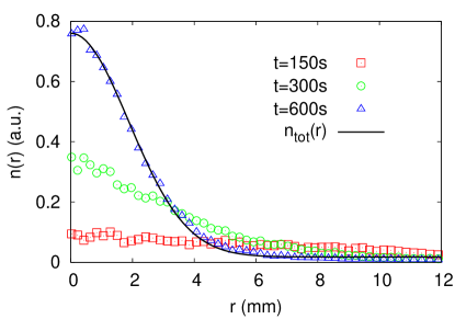
Figure 2: Online version in colour. Evolution of the experimental radial population density $n_{exp}(r,t)$ (in arbitrary units) for the experiment at frequency $f=7\,Hz$ a time $t=150\,s$ (red squares), $t=300\,s$ (green circles) and at time $t=600\,s$ (blue triangles) as a function of the distance from the cylinder axis $r$. The black solid line represents the theoretical prediction for the total density in stationary conditions $n_{tot}(r)=n_{s}(r)+b$ with $n(r)$ given by (11). The cell’s parameters are $v_{s}=0.1\,mm/s$, $B=7.5\,s$, $d_{r}=0.067\,rad/s$ ($\lambda=1.0$). The background parameter is fitted to $b=0.017$ which corresponds to $\beta=N_{b}/N_{s}\simeq 1.1$.

Therefore, the experimental density $n_{exp}(r)$ will be compared with the total density, given by the superposition of the two populations, $n_{tot}(r,t)=n(r,t)+b$ because, thanks to the dilute concentration, we can assume that the non-motile population does not interfere with the motion of the swimming population. The total number of cells $N_{tot}$ becomes

$$N_{tot}=N_{s}+N_{b}=2\pi H\int_{0}^{R}rn(r,t)dr+H\pi R^{2}b\,.$$ (13)

By using the total population density, the stationary average distance (12) becomes

$$\langle r\rangle=\frac{1+c^{2}\beta}{\langle r\rangle_{s}^{-1}+2c\beta R^{-1}}$$ (14)

where $\langle r_{s}\rangle$ is given by (12), $\beta\equiv N_{b}/N_{s}$ is the ratio of the two populations and $c=R_{v}/R=2/3$ is a numerical correction due to the fact that the experimental radial distribution is sampled only up to $R_{v}<R$.

Figure 2 shows the time evolution of the experimental radial population distribution for the experiment at $f=7\,Hz$. As one can see, the population of swimming cells progressively concentrates around the axis of the cylinder ($r=0$). After the last time shown in the plot ($t=600\,s$, which corresponds to the images shown in Fig. 1) the distribution remains statistically stationary. The theoretical asymptotic distribution (11) is used to fit the stationary distribution. As in (11) the cell’s parameters enter only in the combinations $v_{s}B$ and $Bd_{r}=\lambda$ we cannot use the stationary distribution to fit all the parameters. We have therefore chosen to fix two of the parameters as given by literature i.e. $v_{s}=100\,\mu m/s$ and $d_{r}=0.067\,$rad$/s$ Harris (2009); Williams and Bees (2011), and to use the orientation time $B$ as a fitting parameter. The resulting value, $B=7.5\,s$, is compatible with estimations for Chlamydomonas Yoshimura et al. (2003); Roberts (2006). We remark however that, as clear from the above discussion, other combinations of the parameters are possible. The theoretical asymptotic distribution (11), with the correction of the background term ($b=0.017$), fits very well the experimental data.

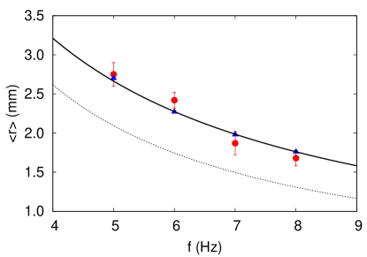
Figure 3: Online version in colour. Stationary radius of cell population, $\langle r\rangle$ from experimental distribution (15) (red circles) and theoretical prediction, both in the absence of non-motile background cells (12) (dotted line) and with background contribution (14) with $\beta=1.1$ (solid line). The error bars on the experimental data are obtained from the temporal fluctuations of the asymptotic radius for $t>600\,s$. The blue triangles represent the asymptotic values obtained from numerical simulations of a population of $10^{5}$ swimmers as explained in Section II.5.

Figure 3 shows the theoretical and experimental values of the mean radius $\langle r\rangle$ in stationary conditions. The experimental stationary radius is obtained by computing, for different values of the rotation frequency $f$, the time evolution of

$$\langle r(t)\rangle_{exp}=\frac{\int_{0}^{R_{v}}rn_{exp}(r,t)dr}{\int_{0}^{R_{v}}n_{exp}(r,t)dr}$$ (15)

and looking at the plateau that can be observed at long time values (see Fig. 4). Figure 3 shows both the theoretical value in the absence of background (12), which clearly underestimates the asymptotic radius, and the expression (14) corrected with the background coefficient $\beta=1.1$. We remark that the theoretical line in Fig. 3 is obtained without free parameters, as $\beta$ is fitted from the asymptotic distribution $n_{s}(r)$ for a single rotation frequency (Fig. 2).

By using the numerical method discussed in Section II.5 it is possible to obtain the time evolution of the radial population density $n(r,t)$ and of the mean radius. We remark that the time evolution of the population density depends on a different combination of the parameters with respect to the stationary distribution. Therefore, the ability to reproduce the experimental dynamics from the numerical integration of (3-6), without additional fitting parameters, is both a test of the validity of the mathematical model and of the chosen set of parameters. The time evolution of the mean radius is shown in Fig. 4 for the four different values of rotation and with the contribution of the background term $b=0.017$ as for the theoretical analysis. The presence of an initial plateau of almost constant $\langle r\rangle$ (which is more evident for the experiments at lower frequencies) is a consequence of the fact that the average in (15) is taken over the inner cylinder of radius $R_{v}<R$ (indeed, the analysis of the numerical data up to $R$ shows that the plateau disappears). The quality of the agreement between the theoretical prediction and the experimental evolution of the mean radius is remarkable.

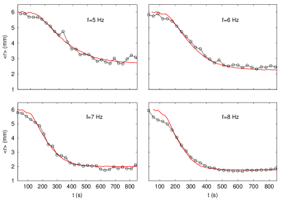
Figure 4: Online version in colour. Cell population radius as a function of time measured in experiments (symbols) and in simulations with background $\beta=1.1$ (red solid line). Model parameters as in Fig. 2. We introduced in the numerical data a time shift $\Delta t$ in the range $10-50\,s$ as the initial phase of spin-up is not reproduced by the simulations.

IV Conclusion and discussion

We have studied the centripetal focusing of gyrotactic microalgae around the axis of a rotating container. By using a refined model of gyrotactic motion (which takes into account the effect of fluid acceleration on cell orientation) we derived an effective equation for the evolution of the population density inside the container. The analytical predictions for the stationary distribution and its characteristic size reproduce accurately the experimental data obtained from a population of C. augustae in a vessel rotating with different angular velocities. The time evolution of the distribution is obtained by stochastic simulations of the Fokker-Planck equation. Also in this case the results reproduce accurately the experimental data without additional free parameters.

One of the motivations of our study is to better understand the behavior of gyrotactic organisms in a turbulent environment (natural or artificial) characterized by strong region of vorticity. Indeed, recent numerical simulations have shown that gyrotactic swimmers are able to concentrate in regions of high vorticity even if these regions are very localized and ephemeral, as in the case of homogeneous turbulence De Lillo et al. (2014). In this perspective, the vertical solid body rotator has to be considered as a “toy model” of a turbulent vortex for which analytical prediction are possible. Similar configurations of uniform vorticity have been studied recently and proposed for laboratory experiments in theoretically controlled conditions Thorn and Bearon (2010); Pedley (2015). On the basis of our results, artificial turbulent flows could be designed to optimize the trapping of swimming cells in specific regions.

More in general, understanding the interplay between swimming and fluid transport is crucial to rationalize phytoplankton ecology Reynolds (2006); Kiørboe (2008) and also for industrial applications. For example, many (motile) microalgae are cultured in photobioreactors to be commercially used as nutrients, for biofuels production or for cosmetic industry Borowitzka (1999). As bioreactors work both in laminar and turbulent fluid motion Croze et al. (2013), a better understanding the interaction between fluid motion and swimming is fundamental to optimize efficiency.

Appendix A Solution of the deterministic model

The radial evolution of the deterministic model (3)-(6) can be solved using the equilibrium hypothesis (i.e. assuming that $\dot{\bf p}=0$, which should be valid for times much larger than $B$). The symmetries of the problem suggest that ${\bf p}_{r}=\mathrm{p}_{r}(r)\hat{\bm{r}}$ and $\mathrm{p}_{z}=\mathrm{p}_{z}(r)$, with $\mathrm{p}^{2}_{r}(r)+\mathrm{p}^{2}_{z}(r)=1$. To find the expressions for $\mathrm{p}_{r}$ and $\mathrm{p}_{z}$, it is convenient to multiply (5) by ${\bf p}_{r}$, using ${\bf p}_{r}^{\perp}\cdot{\bf p}_{r}=0$, one obtains ${\bf p}_{r}=-(\gamma\bm{r})/\sqrt{1+(\gamma r)^{2}}$ and $\mathrm{p}_{z}=1/\sqrt{1+(\gamma r)^{2}}$ whose physical interpretation is transparent: ${\bf p}$ aligns in the direction opposite to the total acceleration (see Eq. (7)).

Multiplying (3) by $\bm{r}$ we obtain that the radial distance evolves according to

$$\dot{r}=-\gamma v_{s}\frac{r}{\sqrt{1+(\gamma r)^{2}}}\,.$$ (16)

When $\gamma r\ll 1$, Eq. (16) reduces to $\dot{r}=-\gamma v_{s}r$ implying an exponential decay of the distance from the axis, see Eq. (8). When $\gamma r\gg 1$, Eq. (16) reduces to $\dot{r}\approx-v_{s}$ so that we have $r(t)=r(0)-v_{s}t$, i.e. a linear decrease of the distance from the axis of rotation. For generic $\gamma r$, Eq. (16) is solved by

$$\frac{r}{r_{0}}\frac{1+\sqrt{1+(\gamma r_{0})^{2}}}{1+\sqrt{1+(\gamma r)^{2}}}e^{\sqrt{1+(\gamma r)^{2}}-\sqrt{1+(\gamma r_{0})^{2}}}=e^{-\gamma v_{s}t}$$ (17)

with $r_{0}=r(0)$ and $r=r(t)$. In typical experimental condition we have $\gamma\approx 65-250$ for $f=4-8$Hz so that for $r_{0}=O(1)$cm we have $(\gamma r)\approx 0.6-2.5$. Therefore, at least at the beginning, there will be deviation from the exponential regime, which shows up in the latest stage of the (deterministic) evolution.

Appendix B Derivation of stationary population density in the presence of rotational diffusivity

Here, we derive the effective drift and diffusion tensor of the advection diffusion equation (10). Then we compute the stationary population density and use it to derive the average distance from the cylinder axis. We detail the method in two dimensions ($d=2$), because algebra is straightforward and closed expressions for the quantities of interest can be found. We then generalize the result to $d=3$, which is the case relevant for the experiment.

B.1 Analytical approximation in $d=2$

As clear from Eq. (3), the fluid velocity causes only rotation around the cylinder axis and does not contribute directly to the radial evolution, which is controlled by swimming. However, rotation and, in particular, the associated centripetal acceleration makes the swimming direction to depend on the radial distance, as clear from Eqs. (5) and (3). We can thus study the problem in two dimensions considering the following dynamics

$$\dot{r} = v_{s}\mathrm{p}_{r}=v_{s}\sin\theta$$ (18)

$$\dot{z} = v_{s}\mathrm{p}_{z}=v_{s}\cos\theta$$ (19)

$$\dot{{\bf p}} = -{\scriptstyle\frac{1}{2B}}(\bm{A}(r)-(\bm{A}(r)\cdot{\bf p}){\bf p})+\bm{\Gamma}_{\mathrm{r}}\,,$$ (20)

with $\bm{A}(r)=\gamma r\hat{\bm{x}}-\hat{\bm{y}}$. The stochastic term $\bm{\Gamma}_{\mathrm{r}}$ represents rotational diffusion used to model stochasticity in the swimming orientation Pedley and Kessler (1987, 1992). By denoting with $r$ and $z$ the $x-$ and $y-$ components of the position vector, respectively, by defining $\theta$ as the angle with the vertical and by posing $\gamma=\Omega^{2}/g$, we will end up with expressions that can be directly used in the $d=3$ case. In $d=2$, Eq. (20) can be conveniently rewritten as a stochastic differential equation for the angle

$$\dot{\theta}=-\frac{1}{2B}(\sin\theta+\gamma r\cos\theta)+\sqrt{2d_{\mathrm{r}}}\eta(t)\,.$$ (21)

Rotational diffusion simply becomes diffusion of the angle, where $\eta$ is white noise of unit variance. By nondimensionalizing the time one easily derives that the orientation distribution is a function of $\gamma$ and of the non-dimensional parameter $\lambda=1/(2Bd_{\mathrm{r}})$, quantifying the cell stability with respect to rotational Brownian motion, a large (small) value of $\lambda$ means that cell orientation is dominated by the bias (rotational diffusion).

For $\gamma=0$, the model describes the evolution of gyrotactic swimmers in a two dimensionional still fluid, a problem for which the effective advection-diffusion equation (10) for the population density has been derived analytically Bearon et al. (2011). Here, we summarize the results and formulas needed in the following (see Appendix A.1 of Ref. Bearon et al. (2011) for a detailed derivation). The stationary distribution of the swimming orientation, i.e. the PDF of $\theta$, is the von Mises probability density function with zero mean, meaning that the average swimming direction is along the vertical,

$$f^{(0)}(\theta)=\frac{1}{2\pi I_{0}(\lambda)}e^{\lambda\cos\theta}\,,$$ (22)

where $I_{k}(\lambda)$ is the modified Bessel function of the first kind and order $k$ Mardia and Jupp (2009). In the above equation and in the following we shall use the superscript ⁽⁰⁾ to denote the $\gamma=0$ results. The population density $n(r,z,t)$ is described by an effective advection-diffusion equation like (10) with drift given by

$$\bm{V}^{(0)}=\!v_{s}\int\!d\theta(\sin\theta,\cos\theta)f^{(0)}(\theta)\!=v_{s}\left(0,\frac{I_{1}(\lambda)}{I_{0}(\lambda)}\right)\,,$$ (23)

and diffusion tensor

$$\mathbb{D}^{(0)}=\frac{v_{s}^{2}}{d_{\mathrm{r}}}\mathrm{Diag}\{D^{(0)}_{\perp}(\lambda),D^{(0)}_{\parallel}(\lambda)\}\,,$$ (24)

where $v_{s}^{2}/d_{\mathrm{r}}$ gives the dimensional contribution; $\perp$ and $\parallel$ label the direction perpendicular and parallel to the bias, respectively. For $\gamma=0$ the swimming direction is biased toward $\hat{\bf y}$. The perpendicular component of the diffusion tensor can be found exactly Bearon et al. (2011)

$$D^{(0)}_{\perp}(\lambda)=\frac{1}{\lambda^{2}}\left(1-\frac{1}{(I_{0}(\lambda))^{2}}\right)\,.$$ (25)

For the parallel one only an approximate expression (not reported here, as not needed in the following) can be found.

When $\gamma\neq 0$, swimming is biased toward a direction that depends on $r$. Our approximation consists in taking $r$ fixed in Eq. (21) and finding the stationary PDF of $\theta$ which will depend on $r$ parametrically. This is a sort of adiabatic approximation, valid when $r$ does not change much in the time scale over which the PDF of orientation becomes stationary. In this way the average swimming direction will depend on $r$ as

$$\hat{\bf b}=\left(\!\frac{-\gamma r}{\sqrt{1\!+\!(\gamma r)^{2}}},\frac{1}{\sqrt{1\!+\!(\gamma r)^{2}}}\!\right)\,,$$ (26)

being at an angle $-\Phi(r)$ with $\Phi(r)=\mathrm{arctan}(\gamma r)$ with respect to $\hat{\bm{y}}$. Since $r$ is assumed fixed, the PDF of $\theta$ will simply be (22) with mean $-\Phi(r)$, i.e.

$$f^{(\gamma)}(\theta;r)=f^{(0)}(\theta+\Phi(r))=\frac{e^{\lambda\frac{(\cos\theta-\gamma r\sin\theta)}{\sqrt{1+(\gamma r)^{2}}}}}{2\pi I_{0}(\lambda)}\,.$$ (27)

Now the drift and diffusion tensor for the $\gamma\neq 0$ case can be obtained from those computed at $\gamma=0$ simply changing to a new (position dependent) frame of reference, essentially we need to rotate the $\gamma=0$ solution at each point matching the vertical with the local biasing direction. Introducing the rotation matrix

$$\mathbb{R}=\begin{pmatrix}\frac{1}{\sqrt{1+(\gamma r)^{2}}}&-\frac{\gamma r}{\sqrt{1+(\gamma r)^{2}}}\\ \frac{\gamma r}{\sqrt{1+(\gamma r)^{2}}}&\frac{1}{\sqrt{1+(\gamma r)^{2}}}\end{pmatrix}\,,$$

the drift can be expressed as

$$\bm{V}^{(\gamma)}=\mathbb{R}\bm{V}^{(0)}=v_{s}\frac{I_{1}(\lambda)}{I_{0}(\lambda)}\,\hat{\bf b}$$ (28)

with $\hat{\bf b}$ given in (26), and the diffusion tensor by $\mathbb{D}^{(\lambda)}=\mathbb{R}\mathbb{D}^{(0)}\mathbb{R}^{T}$. As for the latter we are mainly interested in the radial component which reads

$$D^{(\gamma)}_{rr}=\frac{v_{s}^{2}}{d_{\mathrm{r}}}\frac{D^{(0)}_{\perp}(\lambda)+(\gamma r)^{2}D^{(0)}_{\parallel}(\lambda)}{1+(\gamma r)^{2}}\,.$$ (29)

Now we can approach the advection diffusion equation (10). In particular, because neither the drift nor the diffusion tensor depends on $z$, we can integrate over $z$ and derive the equation for the radial dynamics, which is the one of interest for us,

$$\partial_{t}n-\partial_{r}\left(v_{s}\frac{I_{1}(\lambda)}{I_{0}(\lambda)}\frac{\gamma r\,n}{\sqrt{1+(\gamma r)^{2}}}+D^{(\gamma)}_{rr}\partial_{r}n\right)=0\,.$$ (30)

Imposing stationarity in the above equation, the resulting ordinary differential equation can be integrated obtaining

$$n_{s}(r)=\mathcal{N}\exp(-G(r))$$ (31)

with $\mathcal{N}$ a suitable normalizing constant and

$$G(r)=\frac{d_{\mathrm{r}}}{v_{s}\gamma}\frac{I_{1}}{I_{0}}\frac{\mathcal{D}}{D^{(0)}_{\parallel}}(g(r)-\arctan(g(r)))$$ (32)

with $\mathcal{D}\!=\!\sqrt{(D^{(0)}_{\perp}\!-\!D^{(0)}_{\parallel})/D^{(0)}_{\parallel}}$ and $g(r)\!=\!\sqrt{1\!+\!(\gamma r)^{2}}/\mathcal{D}$ In the limit $(\gamma r)\ll 1$, $G(r)$ can be expanded in

$$G(r)\approx\frac{1}{2}\frac{\gamma d_{\mathrm{r}}I_{1}(\lambda)}{v_{s}D^{(0)}_{\perp}(\lambda)I_{0}(\lambda)}\,r^{2}=\frac{1}{4}\frac{\gamma}{v_{s}BF^{2}_{2}(\lambda)}r^{2}\,,$$ (33)

with

$$F_{2}(\lambda)=\left[\frac{I_{0}(\lambda)-I^{-1}_{0}(\lambda)}{\lambda I_{1}(\lambda)}\right]^{1/2}\,.$$ (34)

Hence the stationary population takes a Gaussian form.

Then we can compute the average radial distance $\langle r\rangle_{s}$ at stationarity as

$$\langle r\rangle_{s}=\frac{\int_{0}^{\infty}rn_{s}(r)dr}{\int_{0}^{\infty}n_{s}(r)dr}=\left(\frac{v_{s}B}{\gamma}\right)^{1/2}\sqrt{\frac{4}{\pi}}F_{2}(\lambda)\,,$$ (35)

in very good agreement with simulations (Fig. 5).

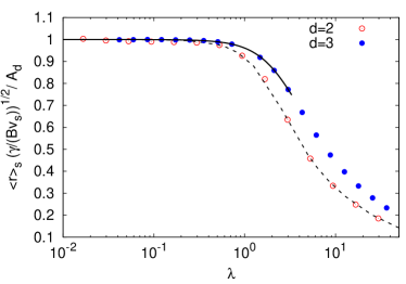
Figure 5: Online version in colour. Comparison between analytical computation of the average radial distance at stationarity and the numerical computation, in both two and three dimensions. Normalized average radial distance at stationarity, $\langle r\rangle_{s}({\gamma}/{v_{s}B})^{1/2}/A_{d}$ (with $A_{2}=\sqrt{4/\pi}$ and $A_{3}=\sqrt{2/\pi}$) vs $\lambda$ compared with the analytical predictions $F_{2}(\lambda)$ and $F_{3}(\lambda)$ given in Eqs. (34) and (41) respectively (lines). For the case $d=3$ the convergence of the recursion relations requires very high accuracy for $\lambda>3$.

B.2 Analytical approximation in $d=3$

The computation in $d=3$ can be performed following step by step the procedure above described for the two-dimensional model.

For $\gamma=0$ in $d=3$, unlike $d=2$, we do not have closed expressions. However, there are exact results expressing the quantities of interest in terms of series in $\lambda=1/(2Bd_{r})$, which have been obtained in Ref. Bearon et al. (2012) (using previous results from Refs. Pedley and Kessler (1987, 1990, 1992)). We briefly summarize the results in the following.

For $\gamma=0$, the orientation distribution is the von Mises-Fisher distribution Mardia and Jupp (2009)

$$f^{(0)}({\bf p})=\mu(\lambda)e^{\lambda{\bf p}\cdot\hat{\bm{z}}}=\mu(\lambda)e^{\lambda\cos\theta}\,,$$ (36)

with ${\bf p}\!\!=\!\!(\cos\phi\sin\theta,\sin\phi\sin\theta,\cos\theta)$ and $\mu(\lambda)\!=\!4\pi\sinh\lambda/\lambda$. The drift has the following exact expression Pedley and Kessler (1987, 1990, 1992)

$$\bm{V}^{(0)}=v_{s}\int d{\bf p}{\bf p}f^{(0)}({\bf p})=v_{s}(0,0,K_{1}(\lambda))$$ (37)

with $K_{1}(\lambda)=\mathrm{coth}\lambda-1/\lambda$; while the diffusion tensor is

$$\mathbb{D}^{(0)}=\frac{v_{s}^{2}}{d_{\mathrm{r}}}\mathrm{Diag}\{D^{(0)}_{\perp}(\lambda),D^{(0)}_{\perp}(\lambda),D^{(0)}_{\parallel}(\lambda)\}$$ (38)

with the two entries perpendicular to the direction of gravity equal. As for the $d=2$ we only need the perpendicular component which takes the form Bearon et al. (2012)

$$D^{(0)}_{\perp}(\lambda)={J_{1}(\lambda)}{\lambda^{-2}}\,,$$ (39)

with the numerator given by the series

$$J_{1}(\lambda)=\frac{4\pi}{3}\lambda\mu(\lambda)\sum_{k=0}^{\infty}\lambda^{2k+1}a_{2k+1,1}\,.$$ (40)

The coefficients $a_{k,n}$ can be obtained by the recursion (see Refs. Bearon et al. (2012); Pedley and Kessler (1990) for details):

$$a_{k+1,n} = -\frac{(n+2)a_{k,n+1}}{(n+1)(2n+3)}+\frac{(r-1)a_{k,n-1}}{r(2r-1)}+\frac{b_{k+1,n}}{n(n+1)}\,,$$

$$b_{k+1,n} = \frac{(2n+1)\Gamma\left(\frac{n+1}{2}\right)\Gamma\left(\frac{n+2}{2}\right)}{\Gamma(n+1)\Gamma\left(4\frac{k-n+3}{2}\right)\Gamma\left(\frac{k+n+4}{2}\right)}\quad\mathrm{if}\;k+n\;\mathrm{odd}$$

and $b_{k+1,n}=0$ otherwise.

With the appropriate rotation matrix, and following the steps described in Appendix B.1, we obtain the very same expressions found in $d=2$ for the radial component of diffusion tensor (see Eq. (29)). In particular, we have that at stationarity in the limit $(\gamma r)\ll 1$ the population density takes the expression (31) with

$$G(r)\!=\!\frac{1}{2}\frac{\gamma r^{2}}{v_{s}BF^{2}_{3}(\lambda)}\quad\mathrm{with}\;F_{3}(\lambda)\!=\!\left[\frac{2J_{1}(\lambda)}{\lambda K_{1}(\lambda)}\right]^{1/2}.$$ (41)

Hence, at stationarity, we find the average radial distance

$$\langle r\rangle_{s}=\frac{\int_{0}^{\infty}rn_{s}(r)dr}{\int_{0}^{\infty}n_{s}(r)dr}=\left(\frac{v_{s}B}{\gamma}\right)^{1/2}\sqrt{\frac{\pi}{2}}F_{3}(\lambda)\,.$$ (42)

in perfect agreement with simulation results (Fig. 5).

References

- Smayda (1997) T. J. Smayda, Limnol. Oceanogr. 42, 1137 (1997).
- Reynolds (2006) C. S. Reynolds, The ecology of phytoplankton (Cambridge University Press, 2006).
- Kiørboe (2008) T. Kiørboe, A mechanistic approach to plankton ecology (Princeton University Press, 2008).
- Elgeti et al. (2015) J. Elgeti, R. G. Winkler, and G. Gompper, Rep. Prog. Phys. 78, 056601 (2015).
- Lieberman et al. (1994) O. S. Lieberman, M. Shilo, and J. Rijn, J. Phycology 30, 964 (1994).
- Cullen (1985) J. J. Cullen, Contrib. Mar. Sci 27, 135 (1985).
- Bollens et al. (2011) S. M. Bollens, G. Rollwagen-Bollens, J. A. Quenette, and A. B. Bochdansky, J. Plank. Res. 33, 349 (2011).
- Wager (1910) H. Wager, Proc. Royal Soc. London B 83, 94 (1910).
- Kessler (1985) J. O. Kessler, Nature 313, 218 (1985).
- Pedley and Kessler (1987) T. J. Pedley and J. O. Kessler, Proc. Royal Soc. B 231, 47 (1987).
- Pedley and Kessler (1992) T. J. Pedley and J. O. Kessler, Annu. Rev. Fluid Mech. 24, 313 (1992).
- Durham et al. (2009) W. M. Durham, J. O. Kessler, and R. Stocker, Science 323, 1067 (2009).
- Durham et al. (2013) W. M. Durham, E. Climent, M. Barry, F. De Lillo, G. Boffetta, M. Cencini, and R. Stocker, Nature Comm. 4, 2148 (2013).
- Zhan et al. (2014) C. Zhan, G. Sardina, E. Lushi, and L. Brandt, J. Fluid Mech. 739, 22 (2014).
- Fouxon and Leshansky (2015) I. Fouxon and A. Leshansky, Phys. Rev. E 92, 013017 (2015).
- Gustavsson et al. (2015) K. Gustavsson, F. Berglund, P. Jonsson, and B. Mehlig, arXiv preprint arXiv:1501.02386 (2015).
- Malkiel et al. (1999) E. Malkiel, O. Alquaddoomi, and J. Katz, Measur. Sci. Tech. 10, 1142 (1999).
- La Porta et al. (2001) A. La Porta, G. Voth, A. Crawford, J. Alexander, and E. Bodenschatz, Nature 409, 1017 (2001).
- Biferale et al. (2005) L. Biferale, G. Boffetta, A. Celani, A. Lanotte, and F. Toschi, Phys. Fluids 17, 021701 (2005).
- De Lillo et al. (2013) F. De Lillo, M. Cencini, G. Boffetta, and F. Santamaria, J. Turbulence 14, 24 (2013).
- De Lillo et al. (2014) F. De Lillo, M. Cencini, W. M. Durham, M. Barry, R. Stocker, E. Climent, and G. Boffetta, Phys. Rev. Lett. 112, 044502 (2014).
- Andersen (2005) R. Andersen, Algal culturing techniques (Elsevier, 2005).
- Chini Zittelli et al. (2000) G. Chini Zittelli, R. Pastorelli, and M. R. Tredici, J. Appl. Phycology 12, 521 (2000).
- Greenspan and Howard (1963) H. Greenspan and L. Howard, J. Fluid Mech. 17, 385 (1963).
- Harris (2009) E. H. Harris, The chlamydomonas sourcebook, Vol. 1 (Academic Press, 2009).
- Pedley and Kessler (1990) T. Pedley and J. Kessler, J. Fluid Mech. 212, 155 (1990).
- O’Malley and Bees (2012) S. O’Malley and M. A. Bees, Bull. Math. Biol. 74, 232 (2012).
- Hill and Häder (1997) N. Hill and D. Häder, J. Theor. Biol. 186, 503 (1997).
- Frankel and Brenner (1989) I. Frankel and H. Brenner, J. Fluid Mech. 204, 97 (1989).
- Bearon et al. (2011) R. Bearon, A. Hazel, and G. Thorn, J. Fluid Mech. 680, 602 (2011).
- Bearon et al. (2012) R. Bearon, M. Bees, and O. Croze, Phys. Fluids 24, 121902 (2012).
- Hill and Bees (2002) N. Hill and M. Bees, Phys. Fluids 14, 2598 (2002).
- Manela and Frankel (2003) A. Manela and I. Frankel, J. Fluid Mech. 490, 99 (2003).
- Bees et al. (1998) M. A. Bees, N. A. Hill, and T. J. Pedley, J. Math. Biol. 36, 269 (1998).
- Williams and Bees (2011) C. Williams and M. Bees, J. Fluid Mech. 678, 41 (2011).
- Yoshimura et al. (2003) K. Yoshimura, Y. Matsuo, and R. Kamiya, Plant Cell Physiol. 44, 1112 (2003).
- Roberts (2006) A. M. Roberts, Biol. Bull. 210, 78 (2006).
- Thorn and Bearon (2010) G. J. Thorn and R. N. Bearon, Phys. Fluids 22, 041902 (2010).
- Pedley (2015) T. Pedley, J. Fluid Mech. 762, R6 (2015).
- Borowitzka (1999) M. A. Borowitzka, J. Biotechnology 70, 313 (1999).
- Croze et al. (2013) O. A. Croze, G. Sardina, M. Ahmed, M. A. Bees, and L. Brandt, J. Roy. Soc. Interface 10, 20121041 (2013).
- Mardia and Jupp (2009) K. V. Mardia and P. E. Jupp, Directional statistics, Vol. 494 (John Wiley & Sons, 2009).