Cell identification in whole-brain multiview images of neural activation maps

Abstract

We present a scalable method for brain cell identification in multiview confocal light sheet microscopy images. Our algorithmic pipeline includes a hierarchical registration approach and a novel multiview version of semantic deconvolution that simultaneously enhance visibility of fluorescent cell bodies, equalize their contrast, and fuses adjacent views into a single 3D images on which cell identification is performed with mean shift.

We present empirical results on a whole-brain image of an adult Arc-dVenus mouse acquired at $4\text{\,}\mathrm{\SIUnitSymbolMicro m}$ resolution. Based on an annotated test volume containing 3278 cells, our algorithm achieves an $F_{1}$ measure of 0.89.

1 Introduction

Understanding the basic principles of brain dynamics is one of the biggest challenges for contemporary science. The presence of a complex network of short- and long-range connections between neurons results into a tight functional coupling between different areas of the brain, since each single neural cell can be elicited or inhibited by a cohort of neurons distributed throughout the whole encephalon. Therefore, different brain states associated with specific behavioral or cognitive states result in distinct patterns of neuronal activation alivisatos_brain_2012 . The technical ability to map such patterns with single-cell resolution would provide a clearer view of brain activity and of its relation with the underlying anatomical architecture oh_mesoscale_2014 .

State-of-the art techniques for in vivo neuronal activity imaging are usually limited by coarse resolution or restricted field of view. For instance, functional magnetic resonance imaging (fMRI) can monitor neuronal activity in vivo throughout the whole brain, but with a spatial resolution too coarse to distinguish single cells logothetis_what_2008 . On the other hand, electrophysiology recordings or two-photon optical functional imaging allow inspecting neuronal activity with high resolution, but only on a small area kerr_imaging_2008 . To overcome these limitations, and afford brain-wide cellular-resolution neuronal activation maps, a complementary approach based on ex vivo mapping of immediate early genes (IEGs) expression has been proposed in the recent years vousden_whole-brain_2014 ; kim_mapping_2015 . Indeed, several transgenic mouse strains have been developed showing expression of a fluorescent protein under the promoter of one of the two main IEGs (Arc and c-Fos), thus resulting in fluorescent tagging of activated neurons barth_visualizing_2007 ; eguchi_vivo_2009 ; guenthner_permanent_2013 . Since endogenous fluorescence is preserved after tissue fixation, high-throughput ex vivo microscopy and image analysis can be used to quantify expression of one IEG with cellular resolution across the whole mouse brain. Vousden vousden_whole-brain_2014 and Kim kim_mapping_2015 , together with their co-workers, demonstrated this approach by using Serial Two-Photon sectioning tomography (STP) ragan_serial_2012 and 2D cell localization based either on 2D segmentation vousden_whole-brain_2014 or convolutional neuronal networks kim_mapping_2015 . Nevertheless, since STP typically images only one optical section ($\approx$1\text{\,}\mathrm{\SIUnitSymbolMicro m}$$) every $50-$100\text{\,}\mathrm{\SIUnitSymbolMicro m}$$, only a small fraction of the brain volume ($\approx 1-2$ %) was actually sampled in these works.

Full volumetric imaging of macroscopic specimens with micrometric resolution is possible using light sheet microscopy (LSM) coupled with tissue clearing dodt_ultramicroscopy:_2007 ; silvestri_confocal_2012 ; costantini_versatile_2015 . However, residual scattering of light and other artifacts due to imperfect sample clearing introduce quite large variability of quality and contrast in LSM images, thus challenging state-of-the-art image analysis methods. For example, cell detection procedures like NeuroGPS quan_neurogps:_2013 or DeadEasy forero_deadeasy_2009 are based on morphological analysis which is preceded by binarization. Finding a correct binarization threshold in LSM images is hard because even spatially close structures may have significantly different intensities. To tackle the quality variability problem, we recently developed an image processing method (Semantic Deconvolution, SD) to enhance the structures of interest (fluorescent cell bodies) and equalize their contrast across the entire image frasconi_large-scale_2014 . SD is based on a supervised learning approach. Given knowledge of true cell coordinates in a small training volume, a neural network is trained to convert the original images into “ideal images” where cell bodies are represented as 3D truncated Gaussians, and everything else is dark. Once SD has been applied to the images, simple localization algorithms like mean shift can reach very high performance scores frasconi_large-scale_2014 .

When imaging entire or even half mouse brains, the effects of light scattering can be so strong that some regions of the sample result almost completely dark when imaged with LSM (see Fig. 1). Since the spatial position of the “dark” and “bright” regions depends on the orientation of the sample with respect to the excitation and detection optics (see Fig. 1), the specimen can be rotated to obtain a collection of images in which every part of the sample is in a “bright” region at least once. Multiview LSM is indeed quite common in non-cleared specimens, like embryos huisken_optical_2004 ; keller_reconstruction_2008 , and a number of algorithms for alignment and fusion of multiple views have been developed in the last years swoger_multi-view_2007 ; rubio-guivernau_wavelet-based_2012 ; preibisch_efficient_2014 . Several of these multiview alignment and fusion methods rely on the presence of reference “bright stars” – which in practice are fluorescent nanospheres embedded in a gel surrounding the biological sample – for highly precise alignment rubio-guivernau_wavelet-based_2012 ; preibisch_efficient_2014 . Intensity–based registration algorithms swoger_multi-view_2007 have less requirements in sample preparation, but can introduce alignment artifacts in presence of slight specimen deformations between the acquisition of different views.

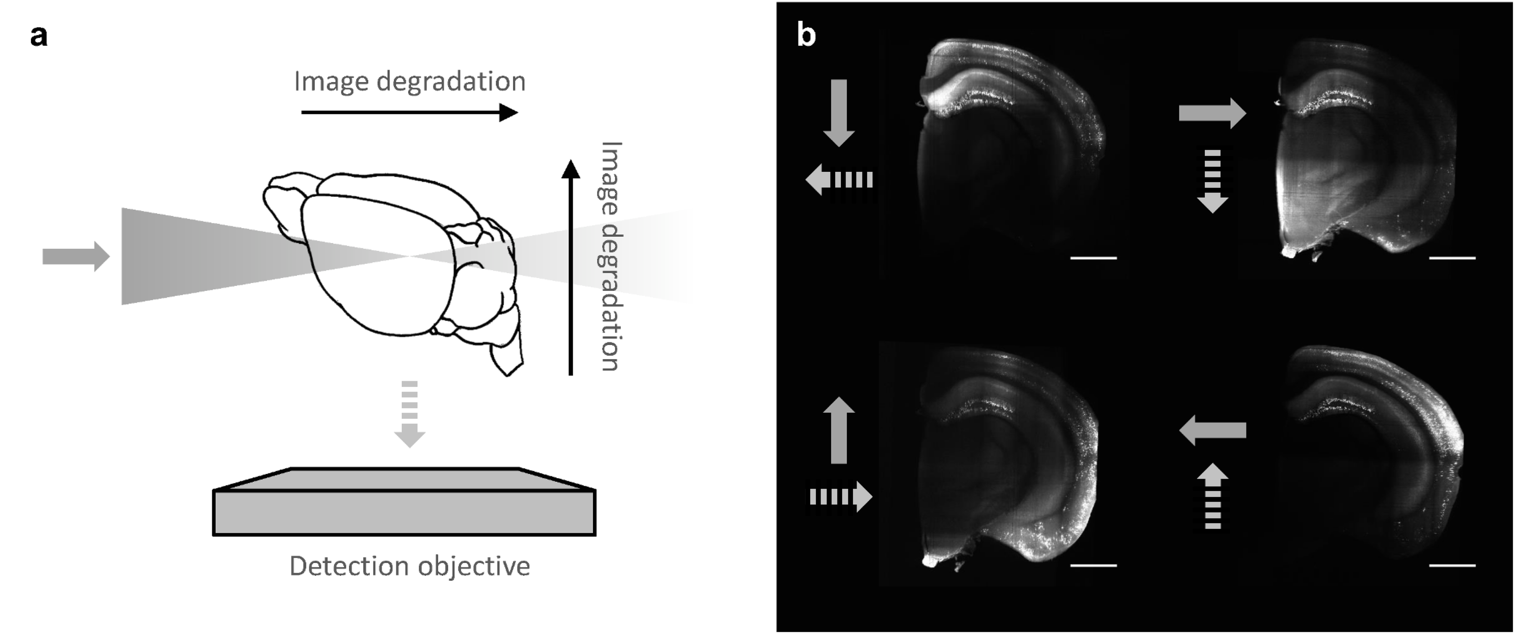
Figure 1: Image degradation in LSM. (a) both excitation (solid arrow) and fluorescence light (dashed arrow) are scattered and absorbed while traveling inside the specimen, leading to image degradation along two orthogonal axes. (b) virtual coronal sections of half a mouse brain imaged with LSM at different angles. The direction of the ingoing excitation light and of the outgoing fluorescence are depicted with solid and dashed arrows, respectively. Scale bars, 1 mm.

Here, we address the problem of extracting the localization maps of Arc-expressing neurons (tagged with the fluorescent protein dVenus eguchi_vivo_2009 ) in multiview LSM images of half a mouse brain. Conventional multiview registration and fusion approaches – which have been devised for samples which are at least one order of magnitude smaller – can be hardly applied with such a large sample: In fact, on the one hand, sample embedding in a gel (which is mandatory for bead-based methods) is not compatible with the clearing protocol (see §2.1). On the other hand, intensity-based registration is limited by the large variability of contrast in the same area for different views (see Fig. 1).

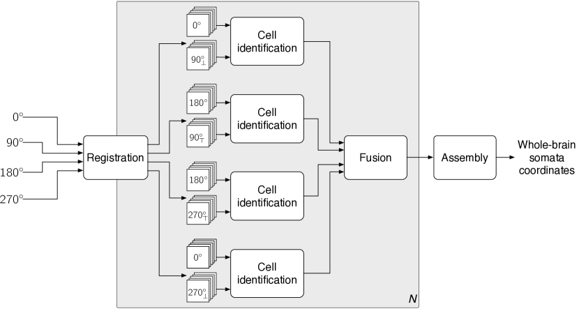
Figure 2: Overall processing pipeline for cell identification. $d^{\circ}_{\perp}$ and $d^{\circ}_{\top}$ (for $d=90,270$) denote substacks from the $d^{\circ}$ view aligned to the $0^{\circ}$ and the $180^{\circ}$ references, respectively.

We thus implemented a two-step registration approach consisting of a coarse global rigid registration, based on manually-picked landmarks, followed by a local rigid alignment maximizing mutual information in pairs of substacks. Pairs of adjacent views are then fused by extending the SD method to manage two images instead of one as input. Afterwards, cell-localization is performed on the semantically deconvolved/fused images. Finally, extracted cell positions from all the pairwise fused images are merged together in a single dataset representing the full distribution of all Arc-expressing neurons in the sample. The entire pipeline is shown in Figure 2.

2 Materials and Methods

2.1 Sample preparation

Adult Arc-dVenus mice eguchi_vivo_2009 were fixed using standard transcardial perfusion with 4% paraformaldehyde (PFA) in phosphate buffered saline (PBS) solution. Brains were extracted from the skull, post-fixed overnight in PFA 4% @ ${4\;}^{\circ}$C, and stored in PBS 4% @ ${4\;}^{\circ}$C. Our clearing protocol is based on the one described by Becker et al. becker_chemical_2012 . Brains were first cut in two halves along the longitudinal fissure, then dehydrated in a graded series of tetrhydrofuran (THF) in water (50%,70%,80%,90%,96%,100% 1 h each, 100% overnight). Afterwards, samples were cleared by immersion in dibenzylether (DBE). DBE was changed three times (2h each) before imaging. Both THF and DBE were previously filtered with aluminum oxide to remove fluorescence-quenching peroxides.

2.2 Imaging

Samples have been imaged in a custom-made confocal light sheet microscope (CLSM) described in detail in silvestri_confocal_2012 . Briefly, light from a $515\text{\,}\mathrm{nm}$ continuous wave laser is scanned by a galvanometric mirror and slightly focused to produce a sheed of light in the sample, following the principle of digital scanned laser light sheet microscopy (DLSM) keller_reconstruction_2008 . The light sheet produced lies at the focal plane of a low-magnification detection objective (Leica HI PLAN 4X, numerical aperture 0.10), which collects emitted fluorescent light. A de-scanning imaging system in the detection optical path creates a fixed image of the scanning excitation laser line; at the position of this image a linear spatial filter (slit) is placed to remove out-of-focus and scattered light. A third scanning mirror, inserted in a further imaging lens system, reconstructs a bi-dimensional image on the chip of a high-sensitivity camera. A fluorescence filter placed inside this third scanning system blocks all stray excitation light, allowing only fluorescence emission to be collected by the camera. The sample chamber is mounted on a motorized system allowing specimen motion along 3 perpendicular axis and rotation along the axis perpendicular to both the excitation and the detection directions.

The transfer function of the microscope (Point Spread Function, PSF) is quite anisotropic as its width along the detection axis is 3-4 times larger than on the illumination plane silvestri_confocal_2012 . Therefore, cell bodies usually appear as prolate ellipsoids rather than spheres; the orientation of the longer axis of the ellipsoid depends on the angle from where the volume is imaged (see Supplementary Figure 1). Although the resolution is anisotropic, we chose to use an isotropic sampling volume (voxel) of $4\text{\,}\mathrm{\SIUnitSymbolMicro m}$ side. This choice simplifies multiview fusion as no resampling of the data is needed. Several parallel stacks were collected to cover the entire sample volume, since the field of view of the camera resulted in $\approx 2\times$2\text{\,}{\mathrm{mm}}^{2}$$. A small overlap of about $200\text{\,}\mathrm{\SIUnitSymbolMicro m}$ was introduced between adjacent image stacks to allow subsequent stitching using the TeraStitcher software bria_terastitcher-tool_2011 . Samples were imaged from 4 different angles separated by $90^{\circ}$.

2.3 Multiview Coarse-to-Fine Registration

There are several brain regions which are well visible in one view only, and several other regions where contrast is not equally high in all views. Thus, registering the images and exploiting the complementary information in the four views can be expected to improve cell identification accuracy.

In spite of the fact that the four views were obtained by simply rotating the specimen at four different angles, a rigid transformation is not sufficient to obtain a good registration. This is mainly due to the incremental errors introduced during the initial stitching of the CLSM tiles (the TeraStitcher software bria_terastitcher-tool_2011 was used for this purpose) which produce slight but noticeable non-linear deformations of the images. The solution suggested in the present work is a simple hierarchical algorithm that starts from a coarse rigid transformation and then performs local refinements to reduce the misalignments due to non-rigid deformations.

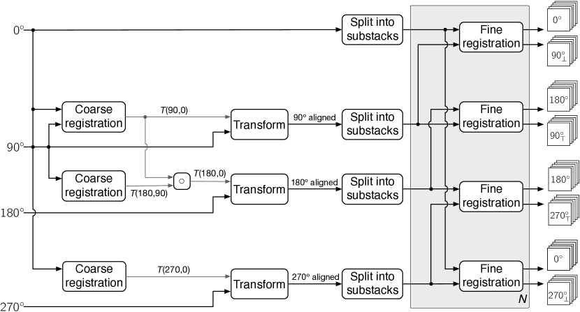
Figure 3: Registration pipeline. The inputs are four stitched volumes from orthogonal views. $T(a,b)$ are the coarse transformations mapping from view $a$ to view $b$. The shaded box is executed in parallel for all substacks. At the end, four paired sets of substacks associated with adjacent views are produced.

The hierarchical registration pipeline is shown in Figure 3. The coarse registration stage is run three times in order to align the target views $90^{\circ}$, $180^{\circ}$, and $270^{\circ}$ to the reference $0^{\circ}$ view. As detailed below, coarse registration is based on a small set of manually annotated fiducial points. The registrations $90^{\circ}$ to $0^{\circ}$ and $270^{\circ}$ to $0^{\circ}$ can be performed directly. However, opposite views $0^{\circ}$ and $180^{\circ}$ share an insufficient portion of visible brain image to allow the extraction of fiducial points. Hence, we first registered $180^{\circ}$ to $90^{\circ}$, obtaining a transformation $T(180,90)$, and then computed the transformation $T(180,0)$ as the composed transformation $T(90,0)\circ T(180,90)$.

In the middle of the registration pipeline, the four 3D volumes are split into $N$ overlapping substacks as in frasconi_large-scale_2014 and subsequent operations (shaded area in Figure 3) are performed independently on adjacent pairs of substacks. Splitting large volumes into smaller portions has several advantages:

• the transformation required for image registration is approximately rigid at the local level (see §2.3);

• operations on substacks can be carried out in parallel on a computing cluster;

• the regional illumination variability can be factored out by performing thresholding at the substack level (see §2.8);

• the running time of the mean shift algorithm used for somata identification (see §2.8) is significantly reduced by operating at the local level.

The fine registration stage takes substacks from the $0^{\circ}$ and the $180^{\circ}$ views as the reference images and substacks from the $90^{\circ}$ and the $270^{\circ}$ views as the target images (i.e., it is run four times in total). Fine registration between opposite views is not run during this processing stage. This is for two reasons. First, for most substacks too few cells are visible in both opposite views. Second, as explained in § 2.2, spheres are deformed into prolate ellipsoids whose longer axis orientation is the same for opposite views ($0^{\circ}$-$180^{\circ}$ and $90^{\circ}$-$270^{\circ}$), where the detection axis lies along the same line (see Supplementary Figure 1). Our scheme ensures that any pair of aligned substacks has a consistent orientation of deformation and this is useful to help generalization of the neural network in the subsequent semantic deconvolution step.

The fine registration module is preceded by a test checking for black regions. If both views are black the pipeline is terminated returning an empty list for that pair of substack views. In the following we provide additional details on the coarse and fine registration modules.

Coarse Registration.

In this step, we estimate the 3D rigid transformation between pairs of views of whole brain images. For this purpose, we manually annotated the four views with 15 corresponding markers using the Vaa3D software peng_v3d_2010 . While in principle just three correspondences are sufficient to estimate a 3D rigid transformation, a greater number is required to compensate the unavoidable imprecisions in the human-created landmarks due to low resolution, high anisotropy, and illumination differences. In order to improve the robustness of the solution, we applied the RANSAC outlier rejection procedure fischler_random_1981 to the list of landmark correspondences. The resulting absolute orientation problem was solved using the Arun et al.method arun_least-squares_1987 , which uses a closed-form optimization algorithm and 3D points as registration features. This technique solves a constrained least squares problem, based on the computation of the Singular Value Decomposition (SVD) on a matrix derived from the rotation component of the rigid transformation. The estimated rigid transformation is finally applied to the whole 3D volume. Voxel intensities in the output image are assigned using the nearest neighbor interpolation algorithm.

Fine Registration based on Mutual Information Metric.

After coarse registration, a local fine-tuning procedure was employed to improve the quality of the alignment. For this purpose, we split the whole brain image into small substacks of size $91\times 90\times 90$ and registered each pair of substacks by maximizing a mutual information metric viola_alignment_1997 . In particular, we used the approach proposed by Mattes et al.mattes_nonrigid_2001 where the spatial samples used to estimate the mutual information are retrieved at the beginning of the process and remain unchanged during the optimization. Assuming that the $g(x|\mu)$ is a rigid deformation from the coordinate frame of the test volume ($V_{T}$) to the reference domain ($V_{R}$), where $\mu$ is the set of transformation parameters to be estimated, $f_{T}(g(x|\mu))$ represents the transformed test volume voxel associated to the reference volume voxel $f_{R}(x)$. To align $f_{R}(x)$ to the transformed test image $f_{T}(x)$, the registration problem consists of determining the set of parameters $\mu^{*}$ that minimize the negative mutual information $S$:

$$\mu^{*}=\mathrm{arg}\min_{\mu}S(f_{R}(x),f_{T}(g(x|\mu))).$$ (1)

This step requires the estimation of the joint and marginal intensity distributions of the reference and test images. Densities were estimated from a representative sample of voxels of both the images, using cubic B-spline Parzen windows for smoothing. We determined that a sample of $10^{5}$ voxels (corresponding to 13 percent of the registered volume) was sufficient. Using more samples would just increase running time without improving the quality of registration.

2.4 Ground truth

Knowledge of the true locations of somata centers is required for training the neural network used in the semantic deconvolution step (see §2.6) and for performance assessment (see §3.2). For this purpose, we manually annotated a random set of 56 substacks of size $91\times 90\times 90$ from different anatomical regions in order to get a rich and diverse collection of cases.

For each view of these substacks, we marked somata that were visible in that view, using a modified version of the Vaa3D program peng_v3d_2010 that incorporates a three-dimensional local cell detector based on mean-shift. Landmarks from different views where subsequently merged using max-weighted bipartite matching galil_efficient_1986 . For this purpose, we created a weighted bipartite graph $G=(V,E)$, with a weight function $w:E\rightarrow\mathbb{R}$ and bipartition $(V_{1},V_{2})$ where $V_{1}$ and $V_{2}$ correspond to manually annotated soma centers in the first and second view, respectively. The weight of edge $(v_{i},v_{j})$, where $v_{i}\in V_{1}$ and $v_{j}\in V_{2}$, was set to $w_{ij}=1/d_{ij}$ being $d_{ij}$ the Euclidean distance between the landmarks $v_{i}$ and $v_{j}$. The merged set of landmarks $M$ was then obtained as follows:

• all unmatched vertices were added to $M$ (these are somata that are visible in one view only)

• matched vertices correspond either to somata that are visible in both views, or to somata that are visible in one view but happen to be close in space; hence, if $d_{ij}\leq d^{*}$ we added to $M$ the middle point between $v_{i}$ and $v_{j}$ and if $d_{ij}>d^{*}$ we added the two landmarks separately; the threshold $d^{*}$ was set to $3$ voxels which is slightly above the maximum soma radius at the image resolution.

2.5 Content-Based Image Fusion

In previous work on LSM imaging, it has been suggested to use content-based weighting in order to fuse images taken from multiple angles into a single isotropic volume preibisch_mosaicing_2008 . This method was applied to whole images following registration (global registration is feasible in preibisch_mosaicing_2008 only thanks to the addition of fluorescent beads to the rigid agarose medium) but it can also be applied to the small substacks used in our setting.

Content-based fusion aims to minimize the blurred parts of each single image, caused by artifacts of the microscopy, and enhance the sharp ones. The adopted strategy consists of computing a weighted average of voxel intensities of each view with their corresponding entropy mask, estimated in the local neighborhood of each voxel. Given two 3D aligned views of the same substack, $V_{i}$ and $V_{j}$ , and their regional entropies $H_{i}(x,y,z)$ and $H_{j}(x,y,z)$, the output fused tensor $V_{fused}$ is computed as follows:

$$V_{fused}(x,y,z)=\frac{100^{H_{i}(x,y,z)}V_{i}(x,y,z)+100^{H_{j}(x,y,z)}V_{j}(x,y,z)}{100^{H_{i}(x,y,z)}+100^{H_{j}(x,y,z)}}$$ (2)

The entropy functions have been used as exponents to underweight the entropy of all the blurred regions of the views that are not completely uniform. The local entropy has been estimated in each voxel from the intensity histogram retrieved by a window centered in that voxel with a side length of $9$ pixels.

2.6 Semantic deconvolution

Images acquired by CLSM generally suffer from significant contrast variability, mainly due to inhomogeneous optical clearing and to different depths that are traveled by the laser beam. The problem is exacerbated when using a high energy laser to penetrate thick tissues, since this can lead to voxel saturation close to the laser entry point. Semantic deconvolution (SD) has been shown to be a very effective preprocessing step in the cell detection pipeline, selectively enhancing contrast for the objects of interest and significantly boosting precision and recall of cell detection frasconi_large-scale_2014 .

SD is a supervised technique consisting of a neural network trained to map native input images into ideal target images where only objects of interest (somata in this case) are preserved and have uniform visibility. The algorithm for constructing the target image can be summarized as follows. Given a set of soma centers $\mathcal{D}=\left\{(x^{(i)},y^{(i)},z^{(i)}),i=1,\dots,n\right\}$ (obtained by manual annotation), we first construct a 3D image with intensity

$$I(x,y,z)=\left\{\begin{array}[]{ll}1&\mbox{if $(x,y,z)\in\mathcal{D}$}\\ 0&\mbox{otherwise}\end{array}\right.$$

and then apply to $I$ a Gaussian filter with kernel standard deviation $\sigma$, obtaining the target image $Y$. To ensure that target blobs remain spatially well separated, the filter is truncated at $2\sigma/3$.

The neural network is trained to map cubic patches of size $s^{3}$ of the original image into corresponding cubic patches of the same size in the target image. The network learns to enhance the visibility of true soma and to reduce the visibility of voxels belonging to other fluorescently labeled structures such as dendrites and axons. After training, the network is applied to the original 3D image $X$ in a convolutional fashion in order to obtain the output image $D$, i.e. for every tuple $(x,y,z)$ of voxel coordinates, we compute

$$D(x,y,z)=\frac{1}{(2s+1)^{3}}\sum_{i,j,k=-s}^{s}F_{x-i,y-j,z-k}(i+1-x,j+1-y,k+1-z)$$ (3)

where $F_{a,b,c}$ denotes the 3D tensor at the output of the neural network when its input consists of the input patch $X(a-s:a+s,b-s:b+s,c-s:c+s)$.

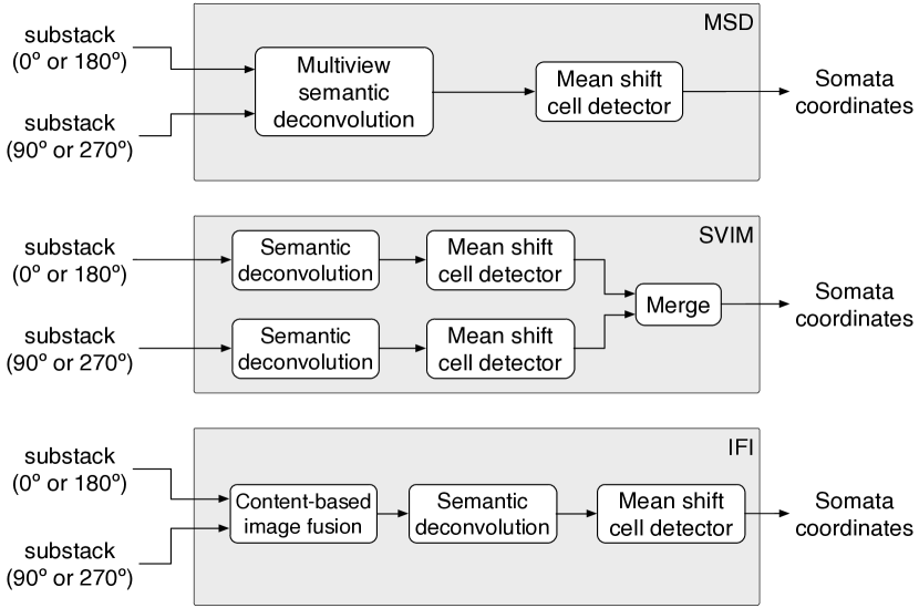
Figure 4: Three alternative options for multiview cell detection

2.7 Multiview cell detection

Dealing with multiview images offers at least three different options for setting up the cell identification pipeline (see Figure 4):

1. Single view identification and merge (SVIM): Identify cells separately in each view and subsequently merge the sets of cells;

2. Identification on fused image (IFI): Fuse views after registration into a single image and perform cell identification on the merged image;

3. Multiview semantic deconvolution (MSD): Develop a specialized SD technique that simultaneously (1) merges different views into a single images and (2) performs selective contrast enhancement;

The pipeline of frasconi_large-scale_2014 (SD followed by mean shift) can be applied immediately to the first two options. One of the contributions of this paper is the development of a novel multiview SD module for enabling the third option. Our results (see Section 3.1) show that MSD outperforms both SVIM and IFI.

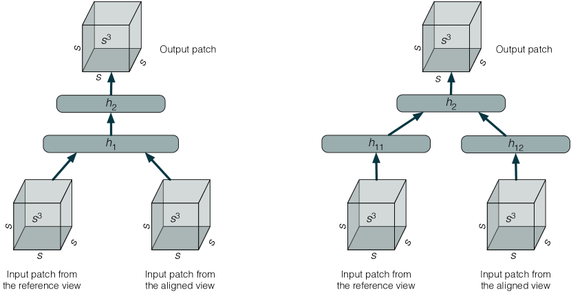
Figure 5: Neural network architectures for multiview semantic deconvolution: flat (left) and columnar (right).

We investigated two alternative neural network architectures for MSD, as shown in Figure 5. In both cases the network takes as input a pair of cubic patches of size $s\times s\times s$. The first patch is taken from a reference substack (either $0^{\circ}$ or $180^{\circ}$) and the second patch is taken from the corresponding registered substack (either $90^{\circ}$ or $270^{\circ}$) following affine transformation. Both patches are taken from the same local coordinates. The network is trained to predict as output the cubic patch of size $s\times s\times s$ in the target image, at the same local coordinates as the input patches. Each output voxel intensity is regarded as the probability that a neural soma occurs at that position. Thus each of the $s^{3}$ outputs of the network has a logistic activation function and the log-loss (or negative cross entropy) is minimized during training:

$$E(W)=\sum_{i}\sum_{j}\sum_{k}y(i,j,k)\log F(i,j,k;W)+(1-y(i,j,k))\log(1-F(i,j,k;W))$$ (4)

where $W$ are the neural network weights, $y$ denotes the target patch, $F$ the patch generated by the neural network, $i$ ranges over the training set substacks, $j$ over the patches in substack $i$, and $k$ over the $s^{3}$ voxels of the patch.

Figure 6: Illustration of multiview semantic deconvolution. Left: $0^{\circ}$ view; middle: $90^{\circ}$ view; right: output image produced by semantic deconvolution. Best viewed by zooming in on the electronic version.

We also experimented alternative ways of training the network. The first procedure uses greedy layer-wise pretraining, using unsupervised learning of restricted Boltzmann machines as originally introduced in hinton_fast_2006 , followed by supervised backpropagation fine-tuning. In this case, logistic units, $f(z)=1/(1+exp(-z))$, are used in all hidden layers. The second procedure does not use pretraining and learns by backpropagation only, using rectified linear units, $f(z)=\max(0,z)$, in all hidden layers. We also experimented with a “masked training” procedure (loosely reminiscent of dropout baldi_dropout_2014 ) where one of the two views is randomly zeroed completely, in order to help the network to produce visible somata in the output image even when they are visible in one of the two views only.

2.8 Somata identification

We formulate the task of somata identification in terms of clustering together voxels belonging to the same soma. This is performed in three steps:

Thresholding.

Voxels with very low intensity are unlikely to be found inside a soma and are therefore discarded in this step. Thresholding offers two advantages: computational efficiency of the subsequent clustering step, and reduction of false positives. Because of the high contrast and illumination variability in different image regions, any global thresholding technique is prone to severe errors (such as suppression of somata in low-visibility regions, if the intensity threshold is too high, or production of too many non-soma clusters, if the intensity threshold is too low). Local thresholding algorithms, on the other hand, are computationally costly, especially for large 3D images. As a reasonable compromise, we operate at the level of substacks and apply a multi-threshold algorithm sahoo_survey_1988 based on maximum entropy kapur_new_1985 . In this way we obtain two substack-local thresholds $\theta_{1}$ and $\theta_{2}$. Voxels with intensity below $\theta_{1}$ are then discarded, yielding a set of foreground voxels $L$.

Seeding.

The clustering procedure starts from a set of carefully selected voxels (seeds) which are good candidate soma centers. In order to be chosen as a seed, a point must satisfy two conditions: it must be a local maximum of the intensity, and must be contained in a region of sufficiently high intensity. Formally, the seeds set is defined as

$$S=\{\vec{p}\in L:m(\vec{p})\}\cap\{\vec{p}\in L:\overline{I}(\vec{p},r)>\theta_{1}\}$$

where $m(\vec{p})$ is true if $\vec{p}$ is a local maximum of the image intensity and $\overline{I}(\vec{p},r)$ is the average local intensity of the image in the $r$-neighborhood of $\vec{p}$, which we define in two alternative ways:

$$\overline{I}(\vec{p},r)=\left\{\begin{array}[]{lll}\displaystyle\frac{\sum_{\vec{q}}I(\vec{q})\mathds{1}\!\left\{\|\vec{p}-\vec{q}\|<r\right\}}{\sum_{\vec{q}}\mathds{1}\!\left\{\|\vec{p}-\vec{q}\|<r\right\}}&{}&\mbox{(hard criterion)}\\ {}\\ \displaystyle\frac{\sum_{\vec{q}}I(\vec{q})\exp(-\|\vec{p}-\vec{q}\|/r)}{\sum_{\vec{q}}\exp(-\|\vec{p}-\vec{q}\|/r)}&{}&\mbox{(soft criterion)}\\ \end{array}\right.$$ (5)

In both cases, $r$ controls the trade-off between false positives and false negatives in the identification procedure defined in the next step: large values reduce the number of seeds, thus decreasing false positives, while small values yield many seeds, decreasing false negatives. In practice we found that the optimal tradeoff occurs when $r$ is close to the expected radius of the fluorescent cell bodies and that the soft criterion yields better results.

Mean shift clustering.

Starting from all elements of $S$, the mean shift algorithm comaniciu_mean_2002 iterates until convergence the following two steps:

1. $$\vec{q}^{(i)}\leftarrow\frac{\sum_{\vec{p}\in L}I(\vec{p})k(\vec{p},\vec{p}^{(i)};b)\vec{p}}{\sum_{\vec{p}\in L}I(\vec{p})k(\vec{p},\vec{p}^{(i)};b)}$$

2. $\vec{p}^{(i)}\leftarrow\vec{q}^{(i)}$

where $I(\vec{p})$ is the intensity of voxel $\vec{p}$ and $k(\vec{a},\vec{b};b)$ is a radial kernel function, parameterized by bandwidth $b$. If $k(\vec{a},\vec{b};b)$ is monotonically non increasing with $\|\vec{a}-\vec{b}\|$, the algorithm is guaranteed to converge. In practice we choose

$$k(\vec{a},\vec{b};b)=\left\{\begin{array}[]{ll}1&\mbox{if $\|\vec{a}-\vec{b}\|\leq b$}\\ 0&\mbox{otherwise}\end{array}\right.$$ (6)

so that every mean corresponds to the “baricenter” (using intensities as masses) of the spherical image patch defined by the kernel. At the end, duplicates are removed resulting in a set $\{\vec{p}^{(i)}\}$ of predicted somata centers. Mean shift has been applied before to cell detection in zebrafish brain but in a very different setting, working in color space and with the purpose of filtering out false positive detections liu_automated_2008 . In our approach mean shift works in coordinate space and is directly responsible for the identification of soma centers.

2.9 Fusion and whole-brain assembly of cell coordinates

The identification module described in §2.8 returns a list of cell body coordinates associated to every pair of adjacent views (i.e. four lists for each substack). When a cell is visible in several views, its coordinates may appear in more than one of these lists. The fusion module in Figure 2 is in charge of removing duplicates and merging results. Duplicates were removed by a merge approach based on the Iterative Closest Point procedure (ICP) Simon:1996:FAS:927342 . In order to give greater importance to the pairs with the smallest distance, the rigid motion estimation was accomplished solving a weighted least squares problem with a quaternion-based method (Horn et al. Horn88closed-formsolution ). After aligning the point clouds, all the computed correspondences were replaced by their midpoint, while all the remaining points (those present in only one list) were preserved.

Concerning the fusion procedure, there are five possible cases to consider, depending on the number of non-empty lists (empty lists are also returned if both views in a substack pair are black). The case are detailed below:

1. All four lists are empty (trivial): return the empty list.

2. Only one list is non-empty (trivial): return that list.

3. If two lists are non-empty there are two sub-cases:

   1. if the non-empty lists come from pairs having the same reference view (two possibilities: $(0^{\circ},90^{\circ}_{\perp})$ and $(0^{\circ},270^{\circ}_{\perp})$, or $(180^{\circ},90^{\circ}_{\top})$ and $(180^{\circ},270^{\circ}_{\top})$) it is sufficient to merge the lists;

   2. if they came from pairs having different references (four possibilities) then it means that some cells are detected in the $0^{\circ}$ and in the $180^{\circ}$ views. In this scenario, we attempt to compute the transformation from $180^{\circ}$ to $0^{\circ}$ using the fine registration procedure of § 2.3. Then, we apply the transformation to the cell coordinates and merge.

4. If there is only one empty list, then two lists comes from the same reference and two lists come from different references. We merge the first two lists, then compute the transformation $180^{\circ}$ to $0^{\circ}$ as above, and then merge the results.

5. If all lists are non-empty then we first merge the lists sharing the same reference, then apply the $180^{\circ}$ to $0^{\circ}$ transformation, and finally merge the results.

Once a unique (possibly empty) list is obtained for each substack, we translate local coordinates into world coordinates in order to assemble the whole-brain list of cell bodies.

3 Results

The images acquired with the method described in 2.2 had size $1823\times 1351\times 2697$ and were split into 15,552 substacks of size $91\times 90\times 90$ with an overlap of 16 voxels. A random subset of 10 manually annotated substacks (see §2.4) was used for training the SD module. The remaining 45 substacks were used to measure the performance of the overall cell identification pipeline.

Unlike other typical machine learning settings, we deliberately used a small volume for training the SD module since somata labeling requires human intervention. Labeling 10 substacks required about 6 hours. This effort is acceptable in relation to the processing time (see §3.6) and to the overall time required to prepare the sample and to carry out imaging. Additionally, we expect that labeling time can be amortized when working on several specimen acquired with the same procedure.

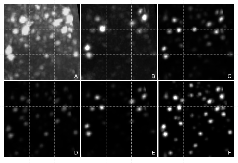
Figure 7: A: original $0^{\circ}$ view. B: original $90^{\circ}$ view. C: content-based image fusion of the two views followed by SD. D: SD on the $0^{\circ}$ view. E: SD on the $90^{\circ}$ view. F: multiview SD.

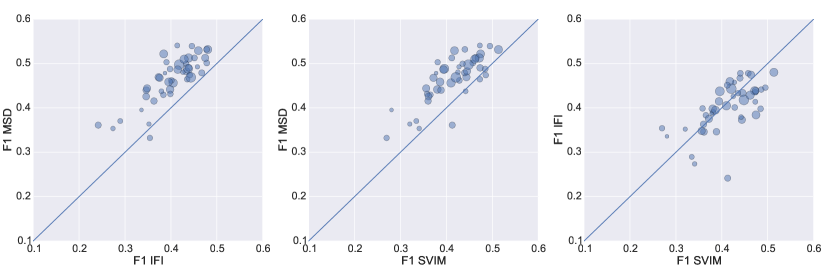
Figure 8: Voxel-level $F_{1}$ measure of semantically deconvolved images. Each dot is one of the 45 test substacks. Dot size is proportional to the number of somata in the substack.

3.1 Target images are better approximated by MSD

In this subsection, we compare the three alternative pipelines of Figure 4 before the cell identification stage. Unlike SVIM and IFI, multiview SD is trained to capture the correlation between 3D patches in the two views. We found that this approach enables a better approximation to the ideal output image. Figure 7 illustrates the differences among SD applied to individual views (as in SVIM), SD on the fused image (as in IFI), and MSD. Visual inspection suggests that some somata are difficult to reconstruct from a single view or from the fused image (this may lead to false negatives at the end of the identification pipeline). In order to quantitatively compare the three approaches, we binarized the images after SD using the maximum entropy threshold $\theta_{1}$ as described in 2.8 and considered the binary classification problem where voxels belong to the negative class iff they are dark in the ideal target image. Since the vast majority of voxels are dark (negative), a very high accuracy (defined as the fraction of correctly predicted voxels) does not necessarily reflect a faithful reconstruction of the target ideal image. For this reason, we consider the $F_{1}$ measure between the binarized target and semantically deconvolved images. $F_{1}$ equals 1 for a perfect classifier. For the SVIM setting, we used the logical “or” between the binarized outputs of SD from the two views. Results are shown in Figure 8, (each dot corresponding to one of the 45 test substacks). While there is no clear winner between IFI and SVIM (p-value of 0.2 from the Wilcoxon signed-rank test), MSD is better than IFI and SVIM on most substacks (p-values are both below $10^{-7}$).

Low $F_{1}$ values indicate that the image fed to the subsequent cell detection stage is likely harder to interpret but $F_{1}$ measures at the level of voxels and at the level of cell detection do not necessarily correlate perfectly: indeed, the voxel-level $F_{1}$ measure does not take into account the different sizes of the visible cell bodies and the spatial distribution of incorrect voxels. Performance of cell detection is detailed in the remainder of this section.

3.2 Measuring the performance of cell detection

For a given substack, we denote by $T$ the set of true somata centers (according to the ground truth) and by $P$ the set of predicted centers. We first match predictions to true centers by creating a weighted bipartite graph $(T\cup P,T\times P)$ with edge weights $w(\vec{t},\vec{p})=1/\|\vec{t}-\vec{p}\|$ for all $\vec{t}\in T$ and $\vec{p}\in P$. We then run the max-weighted bipartite matching algorithm galil_efficient_1986 to obtain a set of matches $M\subset T\times P$. We finally discard any match $(\vec{t},\vec{p})$ if $\|\vec{t}-\vec{p}\|\geq 3.5$ voxels. Unmatched true centers are counted as false negatives (FN), unmatched predicted centers are counted as false positives (FP), and all matches are counted as true positives (TP). We finally report precision $P=\frac{\mathrm{TP}}{\mathrm{TP}+\mathrm{FP}}$, recall $R=\frac{\mathrm{TP}}{\mathrm{TP}+\mathrm{FN}}$, and $F_{1}$ measure $\frac{2PR}{P+R}$.

3.3 Stability with respect to mean shift parameters

One problem faced when designing algorithms for cell detection is that performance may significantly depend on the various parameters of the algorithm. If the optimal value of the parameters needs to be adjusted locally in each image region, the algorithm cannot be easily applied at large scale (this is particularly true for CLSM images because of their inherent contrast variability). Ideally the algorithm should be stable, i.e. (1) performance should not change significantly for small perturbations of the parameters, and (2) the optimal value of parameters should not change significantly in different regions of the image. Our cell identification algorithm depends on the seed ball radius, $r$, and the mean shift bandwidth, $b$. We expect that semantic deconvolution will increase the stability of mean shift with respect to these parameters. In order to verify this speculation, we setup the following experiment, using the SVIM and IFI pipelines of Figure 4, first keeping the SD modules and then suppressing them (i.e. using raw images). In each of the four resulting settings we studied stability as follows. First, we computed the parameters $r^{*}$ and $b^{*}$ that maximize the overall $F_{1}$ measure on the whole available ground truth (45 labeled substacks). Then, for each substack $S_{i}$, we computed the parameters $r^{*}_{i}$ and $b^{*}_{i}$ that locally maximize the $F_{1}$ measure on $S_{i}$.

Results are reported in Table 1 where $F_{1}^{\mathrm{glob}}$ denotes the performance obtained by using the same globally optimal parameters in every substack and $F_{1}^{\mathrm{loc}}$ the performance obtained by using locally optimal parameters. 95% confidence intervals were computed by Monte Carlo simulation, taking 10000 samples from the $F_{1}$ distribution defined by the probabilistic model described in goutte_probabilistic_2005 .

	Raw		SD
	$F_{1}^{\mathrm{glob}}$	$F_{1}^{\mathrm{loc}}$	$F_{1}^{\mathrm{glob}}$	$F_{1}^{\mathrm{loc}}$
SVIM	71.1  [69.8,72.4]	81.0  [80.0,82.0]	88.1  [87.3,88.9]	91.5  [90.8,92.2]
IFI	75.1  [73.9,76.2]	82.8  [81.8,83.8]	87.7  [86.8,88.5]	90.7  [89.9,91.4]
MSD	-	-	89.4  [88.6,90.2]	92.1  [91.4,92.7]

Table 1: Stability of mean shift (95% confidence intervals in brackets).

Both SVIM and IFI result in a large difference between $F_{1}^{\mathrm{glob}}$ and $F_{1}^{\mathrm{loc}}$ when running mean shift on raw images. Differences are significantly reduced if mean shift is run on semantically deconvolved images. Additionally, $F_{1}^{\mathrm{glob}}$ after SD is significantly better than $F_{1}^{\mathrm{loc}}$ on raw images. These results show that SD improves performance significantly and stabilizes it with respect to the parameter values.

3.4 Comparing SVIM, IFI, and MSD

Figure 9 reports precision, recall, and $F_{1}$ measure, when varying the radius of the seed ball, $r$, for the cell identification algorithm. As expected, $r$ controls the tradeoff between false positives and false negatives and therefore precision increases and recall decreases as the criterion for accepting a local maximum as a seed for the mean shift algorithm becomes more stringent. While the precision values of SVIM, IFI, and MSD are relatively close for several $r$’s, recall is significantly better for MSD. In particular, the improvement over SVIM means that the neural network is capable of capturing the correlation between views: learning to combine adjacent views into a single ideal image is more effective than trying to recover two separate ideal images independently from individual views. Interestingly, the optimal tradeoff (best $F_{1}$ measure) is met when $r$ is close to the expected radius of the visible fluorescent cell body (between 1 and 2 voxels in our data). The optimal radius is slightly larger (1.9) in the case of images processed by MSD since MSD tend to produce output images where somata are brighter and larger compared to IFI and SVIM (see Figures 6 and 7).

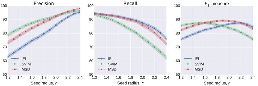
Figure 9: Performance of mean shift after IFI, SVIM, and MSD when changing the seed radius $r$.

We subsequently investigated the effects of changing the kernel bandwidth $b$ (see Eq. 6) on images produced by MSD. While larger values of $b$ tend to push the tradeoff between precision and recall slightly in favor of the former, the $F_{1}$ measure remains statistically indistinguishable (using 95% confidence intervals). Results are reported in Figure 10, where barplots are used for better readability.

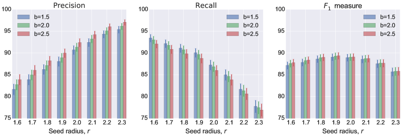
Figure 10: Performance of mean shift after MSD when changing the kernel bandwidth $b$ and the seed radius $r$.

3.5 Effects of the new variants for neural network architecture and training

Semantic deconvolution in frasconi_large-scale_2014 was based on an neural network architecture with pre-trained restricted Boltzmann machines (RBM) in the first two layers, followed by fine tuning by backpropagation. In this paper, besides the multiview extension, we have introduced some architectural variants, namely the use of rectified linear units (ReLU) trained with backpropagation from random initial weights, the columnar architecture shown in Figure 5(b), and the use of a masked training (randomly zeroing one of the two input views). While none of these three variants alone yields a significant performance improvement, their combination does. We compared the two methods in the MSD setting. Results in Figure 11 show a slight improvement in recall and a significant improvement in precision, for all values of $r$. The improvement in terms of $F_{1}$ measure is also significant (using 95% confidence intervals).

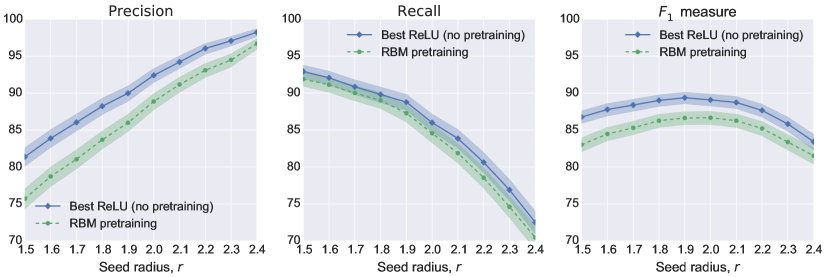
Figure 11: MSD: comparison between the former finely tuned RBM architecture frasconi_large-scale_2014 and the new architecture based on ReLUs, columnar structure, and masked training.

3.6 Mapping neuronal activity at the whole brain scale

We finally applied our method to the whole Arc-dVenus mouse brain images. The registration block (see Figures 2 and 3) ran in about $720\text{\,}\mathrm{min}$ using a cluster of eight quad-core Intel(R) Xeon(R) @2.40GHz CPUs. Multiview semantic deconvolution required $800\text{\,}\mathrm{min}$ using two Tesla K40 GPUs. Finally, cell detection and fusion required $40\text{\,}\mathrm{min}$ on the CPU cluster. Running time of course depends on the number of non-black substacks, which are 4194 out of $15,552$ in the present case. After cell detection, we obtained 3622 non-empty substacks with a total of $91,584$ detected cell bodies. Figure 12 shows the whole activation map obtained with our approach. Activated cells can be largely found in different layers of the cerebral cortex, as well as in the hippocampus and the olfactory bulb. Fewer cells can also be observed in the cerebellar cortex and in deeper brain areas.

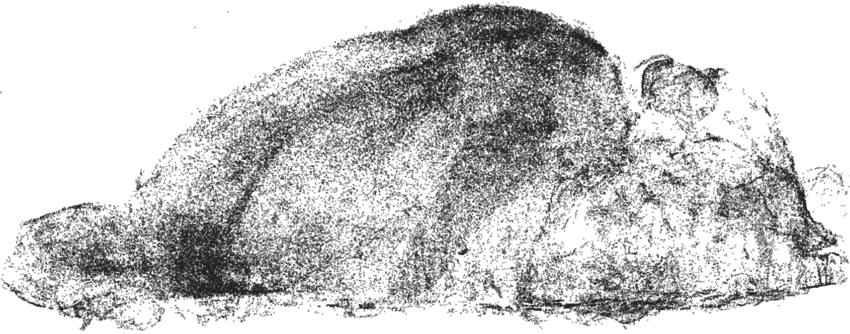
Figure 12: Point cloud showing a whole-brain activation map. $91,584$ active cells have been detected by the software.

4 Conclusions

We have presented a method for identifying cell bodies at the whole-brain scale and applied it to the mapping of neuronal activity in Arc-dVenus mouse. The cell identification approach used in this paper extend previous work frasconi_large-scale_2014 to handle multiview images and some improvements to the neural network used for semantic deconvolution have been presented (use of ReLUs and masked training). Our results indicate that a specially designed multiview semantic deconvolution (MSD) module taking as input two adjacent views simultaneously outperform simpler approach based on content-based image fusion (IFI) or independent processing of the individual views (SVIM). Additionally, we have shown that semantic deconvolution is able to significantly increase performance and stability of the results with respect to changes in the parameter values, thus enabling whole-brain analysis without the need of tuning parameters locally to handle the quality variability problem in CLSM images. Our best performance ($F_{1}$ measure of 89.4) cannot be directly compared to the performance ($F_{1}$ measure of 96.0) we previously attained on GFP-labeled Purkinje cells in the cerebellum. First, resolution in the present study is significantly lower ($4\text{\,}\mathrm{\SIUnitSymbolMicro m}$ vs. $1\text{\,}\mathrm{\SIUnitSymbolMicro m}$ in frasconi_large-scale_2014 ). Second, the use of higher laser power to penetrate the entire brain led to saturation of brightest voxels close to laser entrance point. Third, Purkinje cells have a special spatial arrangement into 3D folia which enabled the use of manifold modeling to filter false positive detections and gain 3 points of $F_{1}$ measure. In the present study, since Arc expression is not related to a specific cell type, no a priori information on spatial arrangement of soma can be exploited. Our current performance is anyway better than that reported in previous work addressing IEGs mapping kim_mapping_2015 .

The approach presented in this Article can provide an important tool to understand whole-brain dynamics in health and disease. To this aim, the soma point clouds obtained need to be mapped on a standard reference atlas to allow quantitative comparison between different subjects. Further, the throughput of the entire experimental pipeline has to be expanded and all the steps, including specimen clearing, imaging, stitching, cell identification and atlasing, needs to be standardized and better integrated. When applied to a significant cohort of mice, in different behavioral tasks and with distinct genetic backgrounds, the methods described here can provide a better understanding of the principles that orchestrate neuronal activity across the entire brain in health and disease.

Availability

The python software used in this paper is included in the 1.1 release of bcfind frasconi_large-scale_2014 and employs portions of pylearn2 goodfellow_pylearn2:_2013 and scikit-learn pedregosa_scikit-learn:_2011 . It is released in open source form under GPL3 and is available from https://github.com/paolo-f/bcfind. The Arc-dVenus mouse brain images are available at https://dataverse.harvard.edu/dataverse/arc_dvenus.

- (1) Alivisatos, A.P., Chun, M., Church, G.M., Greenspan, R.J., Roukes, M.L., Yuste, R.: The brain activity map project and the challenge of functional connectomics. Neuron 74(6), 970–974 (2012). 00203
- (2) Arun, K.S., Huang, T.S., Blostein, S.D.: Least-squares fitting of two 3-D point sets. Pattern Analysis and Machine Intelligence, IEEE Transactions on (5), 698–700 (1987). URL http://ieeexplore.ieee.org/xpls/abs_all.jsp?arnumber=4767965. 02740
- (3) Baldi, P., Sadowski, P.: The dropout learning algorithm. Artificial Intelligence 210, 78–122 (2014). DOI 10.1016/j.artint.2014.02.004. URL http://linkinghub.elsevier.com/retrieve/pii/S0004370214000216. 00025
- (4) Barth, A.L.: Visualizing circuits and systems using transgenic reporters of neural activity. Current opinion in neurobiology 17(5), 567–571 (2007)
- (5) Becker, K., Jährling, N., Saghafi, S., Weiler, R., Dodt, H.U.: Chemical clearing and dehydration of GFP expressing mouse brains. PLoS One 7(3), e33,916 (2012)
- (6) Bria, A., Iannello, G.: TeraStitcher-a tool for fast automatic 3d-stitching of teravoxel-sized microscopy images. BMC bioinformatics 13, 316–316 (2011). 00015
- (7) Comaniciu, D., Meer, P.: Mean shift: A robust approach toward feature space analysis. Pattern Analysis and Machine Intelligence, IEEE Transactions on 24(5), 603–619 (2002). URL http://ieeexplore.ieee.org/xpls/abs_all.jsp?arnumber=1000236. 08448
- (8) Costantini, I., Ghobril, J.P., Di Giovanna, A.P., Mascaro, A.L.A., Silvestri, L., Müllenbroich, M.C., Onofri, L., Conti, V., Vanzi, F., Sacconi, L., others: A versatile clearing agent for multi-modal brain imaging. Scientific reports 5 (2015)
- (9) Dodt, H.U., Leischner, U., Schierloh, A., Jährling, N., Mauch, C.P., Deininger, K., Deussing, J.M., Eder, M., Zieglgänsberger, W., Becker, K.: Ultramicroscopy: three-dimensional visualization of neuronal networks in the whole mouse brain. Nature methods 4(4), 331–336 (2007)
- (10) Eguchi, M., Yamaguchi, S.: In vivo and in vitro visualization of gene expression dynamics over extensive areas of the brain. Neuroimage 44(4), 1274–1283 (2009)
- (11) Fischler, M.A., Bolles, R.C.: Random sample consensus: a paradigm for model fitting with applications to image analysis and automated cartography. Communications of the ACM 24(6), 381–395 (1981). URL http://dl.acm.org/citation.cfm?id=358692. 13241
- (12) Forero, M.G., Pennack, J.A., Learte, A.R., Hidalgo, A.: DeadEasy Caspase: Automatic Counting of Apoptotic Cells in Drosophila. PLoS ONE 4(5), e5441 (2009). DOI 10.1371/journal.pone.0005441. URL http://dx.doi.org/10.1371/journal.pone.0005441. 00016
- (13) Frasconi, P., Silvestri, L., Soda, P., Cortini, R., Pavone, F.S., Iannello, G.: Large-scale automated identification of mouse brain cells in confocal light sheet microscopy images. Bioinformatics 30(17), i587–i593 (2014). DOI 10.1093/bioinformatics/btu469. URL http://bioinformatics.oxfordjournals.org/content/30/17/i587. 00009
- (14) Galil, Z.: Efficient Algorithms for Finding Maximum Matching in Graphs. ACM Comput. Surv. 18(1), 23–38 (1986). DOI 10.1145/6462.6502. URL http://doi.acm.org/10.1145/6462.6502. 00340
- (15) Goodfellow, I.J., Warde-Farley, D., Lamblin, P., Dumoulin, V., Mirza, M., Pascanu, R., Bergstra, J., Bastien, F., Bengio, Y.: Pylearn2: a machine learning research library. arXiv:1308.4214 [cs, stat] (2013). URL http://arxiv.org/abs/1308.4214. 00083 arXiv: 1308.4214
- (16) Goutte, C., Gaussier, E.: A probabilistic interpretation of precision, recall and F-score, with implication for evaluation. In: Advances in information retrieval, pp. 345–359. Springer (2005). URL http://link.springer.com/chapter/10.1007/978-3-540-31865-1_25. 00175
- (17) Guenthner, C.J., Miyamichi, K., Yang, H.H., Heller, H.C., Luo, L.: Permanent genetic access to transiently active neurons via TRAP: targeted recombination in active populations. Neuron 78(5), 773–784 (2013)
- (18) Hinton, G.E., Osindero, S., Teh, Y.W.: A fast learning algorithm for deep belief nets. Neural computation 18(7), 1527–1554 (2006). 02945 XXX
- (19) Horn, B.K.P., Hilden, H., Negahdaripour, S.: Closed-form solution of absolute orientation using orthonormal matrices. JOURNAL OF THE OPTICAL SOCIETY AMERICA 5(7), 1127–1135 (1988)
- (20) Huisken, J., Swoger, J., Del Bene, F., Wittbrodt, J., Stelzer, E.H.: Optical sectioning deep inside live embryos by selective plane illumination microscopy. Science 305(5686), 1007–1009 (2004)
- (21) Kapur, J.N., Sahoo, P.K., Wong, A.K.: A new method for gray-level picture thresholding using the entropy of the histogram. Computer vision, graphics, and image processing 29(3), 273–285 (1985). URL http://www.sciencedirect.com/science/article/pii/0734189X85901252. 02358
- (22) Keller, P.J., Schmidt, A.D., Wittbrodt, J., Stelzer, E.H.: Reconstruction of zebrafish early embryonic development by scanned light sheet microscopy. science 322(5904), 1065–1069 (2008)
- (23) Kerr, J.N., Denk, W.: Imaging in vivo: watching the brain in action. Nature Reviews Neuroscience 9(3), 195–205 (2008)
- (24) Kim, Y., Venkataraju, K.U., Pradhan, K., Mende, C., Taranda, J., Turaga, S.C., Arganda-Carreras, I., Ng, L., Hawrylycz, M.J., Rockland, K.S., others: Mapping Social Behavior-Induced Brain Activation at Cellular Resolution in the Mouse. Cell reports 10(2), 292–305 (2015)
- (25) Liu, T., Li, G., Nie, J., Tarokh, A., Zhou, X., Guo, L., Malicki, J., Xia, W., Wong, S.T.C.: An Automated Method for Cell Detection in Zebrafish. Neuroinformatics 6(1), 5–21 (2008). DOI 10.1007/s12021-007-9005-7. URL http://link.springer.com/article/10.1007/s12021-007-9005-7. 00022
- (26) Logothetis, N.K.: What we can do and what we cannot do with fMRI. Nature 453(7197), 869–878 (2008). 01589
- (27) Mattes, D., Haynor, D.R., Vesselle, H., Lewellyn, T.K., Eubank, W.: Nonrigid multimodality image registration. Proc. SPIE 4322, 1609–1620 (2001). DOI 10.1117/12.431046. URL http://dx.doi.org/10.1117/12.431046. 00226
- (28) Oh, S.W., Harris, J.A., Ng, L., Winslow, B., Cain, N., Mihalas, S., Wang, Q., Lau, C., Kuan, L., Henry, A.M., others: A mesoscale connectome of the mouse brain. Nature 508(7495), 207–214 (2014). 00149
- (29) Pedregosa, F., Varoquaux, G., Gramfort, A., Michel, V., Thirion, B., Grisel, O., Blondel, M., Prettenhofer, P., Weiss, R., Dubourg, V., Vanderplas, J., Passos, A., Cournapeau, D., Brucher, M., Perrot, M., Duchesnay, É.: Scikit-learn: Machine Learning in Python. J. Mach. Learn. Res. 12, 2825–2830 (2011). URL http://dl.acm.org/citation.cfm?id=1953048.2078195. 01780
- (30) Peng, H., Ruan, Z., Long, F., Simpson, J.H., Myers, E.W.: V3d enables real-time 3d visualization and quantitative analysis of large-scale biological image data sets. Nature biotechnol 28(4), 348–353 (2010). 00230
- (31) Preibisch, S., Amat, F., Stamataki, E., Sarov, M., Singer, R.H., Myers, E., Tomancak, P.: Efficient Bayesian-based multiview deconvolution. nature methods 11(6), 645–648 (2014)
- (32) Preibisch, S., Rohlfing, T., Hasak, M.P., Tomancak, P.: Mosaicing of single plane illumination microscopy images using groupwise registration and fast content-based image fusion. In: J.M. Reinhardt, J.P.W. Pluim (eds.) Proc. SPIE Conference on Medical Imaging, vol. 6914, pp. 69,140E–69,140E–8 (2008). DOI 10.1117/12.770893. URL http://dx.doi.org/10.1117/12.770893. 00012
- (33) Quan, T., Zheng, T., Yang, Z., Ding, W., Li, S., Li, J., Zhou, H., Luo, Q., Gong, H., Zeng, S.: NeuroGPS: automated localization of neurons for brain circuits using L1 minimization model. Scientific Reports 3 (2013). DOI 10.1038/srep01414. URL http://www.nature.com/doifinder/10.1038/srep01414. 00007
- (34) Ragan, T., Kadiri, L.R., Venkataraju, K.U., Bahlmann, K., Sutin, J., Taranda, J., Arganda-Carreras, I., Kim, Y., Seung, H.S., Osten, P.: Serial two-photon tomography for automated ex vivo mouse brain imaging. Nature methods 9(3), 255–258 (2012)
- (35) Rubio-Guivernau, J.L., Gurchenkov, V., Luengo-Oroz, M.A., Duloquin, L., Bourgine, P., Santos, A., Peyrieras, N., Ledesma-Carbayo, M.J.: Wavelet-based image fusion in multi-view three-dimensional microscopy. Bioinformatics 28(2), 238–245 (2012). 00015
- (36) Sahoo, P.K., Soltani, S., Wong, A.K.: A survey of thresholding techniques. Computer vision, graphics, and image processing 41(2), 233–260 (1988). URL http://www.sciencedirect.com/science/article/pii/0734189X88900229. 02812
- (37) Silvestri, L., Bria, A., Sacconi, L., Iannello, G., Pavone, F.: Confocal light sheet microscopy: micron-scale neuroanatomy of the entire mouse brain. Optics express 20(18), 20,582–20,598 (2012)
- (38) Simon, D.A.: Fast and accurate shape-based registration. Ph.D. thesis, Pittsburgh, PA, USA (1996). AAI9838226
- (39) Swoger, J., Verveer, P., Greger, K., Huisken, J., Stelzer, E.H.: Multi-view image fusion improves resolution in three-dimensional microscopy. Optics express 15(13), 8029–8042 (2007)
- (40) Viola, P., Wells III, W.M.: Alignment by maximization of mutual information. International journal of computer vision 24(2), 137–154 (1997). URL http://link.springer.com/article/10.1023/A:1007958904918. 03630
- (41) Vousden, D.A., Epp, J., Okuno, H., Nieman, B.J., van Eede, M., Dazai, J., Ragan, T., Bito, H., Frankland, P.W., Lerch, J.P., others: Whole-brain mapping of behaviourally induced neural activation in mice. Brain Structure and Function pp. 1–15 (2014)