Bifurcation analysis of the behavior of partially wetting liquids on a rotating cylinder

Abstract

We discuss the behavior of partially wetting liquids on a rotating cylinder using a model that takes into account the effects of gravity, viscosity, rotation, surface tension and wettability. Such a system can be considered as a prototype for many other systems where the interplay of spatial heterogeneity and a lateral driving force in the proximity of a first- or second-order phase transition results in intricate behavior. So does a partially wetting drop on a rotating cylinder undergo a depinning transition as the rotation speed is increased, whereas for ideally wetting liquids the behavior only changes quantitatively. We analyze the bifurcations that occur when the rotation speed is increased for several values of the equilibrium contact angle of the partially wetting liquids. This allows us to discuss how the entire bifurcation structure and the flow behavior it encodes changes with changing wettability. We employ various numerical continuation techniques that allow us to track stable/unstable steady and time-periodic film and drop thickness profiles. We support our findings by time-dependent numerical simulations and asymptotic analyses of steady and time-periodic profiles for large rotation numbers.

I Introduction

Moffatt Moffatt (1977) first studied film flow on a rotating cylinder to answer the question, “How much honey can be kept on a breakfast knife, while rotating it about its long axis?” and similar closely related questions regarding a number of industrial coating and printing processes where liquid films on rotating cylinders play an important role. These include paper production, paint-application, spit-roasting, molten glass technology and even chocolate manufacturing (see the review by Ruschak Ruschak (1985)). The ability to control technological processes in these and other applications depends on our understanding of the limits that have to be imposed on the amount of liquid or on the rotation speed to ensure that the liquid remains on the cylinder.

Furthermore, Moffatt provides a long-wave model Oron, Davis, and Bankoff (1997) in the overdamped limit (neglecting inertia) that incorporates gravity and viscosity effects but neglects surface tension Moffatt (1977). At about the same time, Pukhnachov developed a model that additionally includes surface tension effects Pukhnachov (1977). Various further extensions were derived that incorporate higher-order terms related to gravity, inertial and centrifugal effects. For a more detailed account see Noakes et al. Noakes, King, and Riley (2006) and Kelmanson Kelmanson (2009). Note that all these models implicitly assume that the liquid ideally wets the cylinder, i.e., they do not incorporate terms that account for wettability.

The equation introduced by Pukhnachov Pukhnachov (1977) and later studied, e.g., in Hinch et al. Hinch and Kelmanson (2003) and Karabut Karabut (2007), is amended by Thiele Thiele (2011) who introduces a Derjaguin (or disjoining) pressure term Oron, Davis, and Bankoff (1997); Starov and Velarde (2009). This allows for a study of the influence of wettability on the drop and film behavior on a rotating cylinder – an influence that becomes particularly important for small cylinders and thin films / small droplets. Furthermore, Ref. Thiele, 2011 introduces an alternative scaling that allows for a straightforward study of the influence of the rotation speed of the cylinder that represents the most important experimental control parameter. The governing long-wave evolution equation for the film thickness profile can then be presented in a form that highlights the analogy between the behavior of films and drops of liquid on a rotating horizontal cylinder and on inclined substrates with regular one-dimensional wettability patterns, i.e., with periodic modulations of the equilibrium contact angle (and sometimes also the precursor film height) Thiele and Knobloch (2006a); Herde et al. (2012); Varagnolo et al. (2013); Sbragaglia et al. (2014).

A central result of Ref. Thiele, 2011 is that the analogy holds, i.e., that film flow and drop motion on the exterior or interior surface of a rotating cylinder on one hand and on a heterogeneous substrate with lateral driving force on the other hand are rather similar. This implies that the bifurcation character of many of the occurring transitions between qualitatively different behaviors of films and drops is similar and corresponding results can be transferred between the systems. In particular, it is found that for partially wetting drops on a rotating cylinder there exists a counterpart of the depinning transition and related dynamics described before for drops on heterogeneous substrates Thiele and Knobloch (2006b); Herde et al. (2012); Beltrame et al. (2011). A depinning transition occurs when a driving force reaches a critical value where a steady structure (e.g., a drop) that is pinned by a heterogeneity (e.g., a less wettable patch or spatially varying gravity) starts to move. This similarity proposes that the rotating cylinder can serve as a model for a more general class of hydrodynamic (and other) depinning processes – a model system that naturally has periodic boundary conditions (BCs) facilitating its analysis. This is important, in particular, when comparing them to the open BCs in models for film deposition at moving contact lines where the transition from the deposition of a homogeneous film to the deposition of line patterns Frastia, Archer, and Thiele (2012); Köpf et al. (2012); Doumenc and Guerrier (2013) can be interpreted as a depinning transition (for a detailed recent discussion of a number of such systems see end of Sec. III of Thiele Thiele (2014) and Sec. 4 of Köpf et al. Köpf and Thiele (2014)).

Ref. Thiele, 2011 mentions in passing that the sequence of qualitative transitions encountered for drops of partially wetting liquids when increasing the rotation speed is not present for ideally wetting liquids. There, the behavior only changes quantitatively with increasing the rotation speed: pendent drops are smeared out into a film in a smooth process, surface waves may appear but no depinning transition can occur. This poses the question how the entire rotation speed-related bifurcation behavior changes when increasing the wettability of the liquid, i.e., decreasing the equilibrium contact angle. A particularly intriguing question is how the global bifurcation related to the depinning of partially wetting drops is eliminated when decreasing the contact angle to small values.

The importance of the interplay of wettability and lateral driving brings the system as well into the context of dynamic wetting transitions that occur for drops sliding down an incline and for films drawn out of a bath Ben Amar, Cummings, and Pomeau (2001); Snoeijer et al. (2008); Ziegler, Snoeijer, and Eggers (2009); Galvagno et al. (2014). Depending on the particular wetting energy (or binding potential), the equilibrium wetting transition Bonn et al. (2002, 2009) is a first- or second-order phase transition where above the critical value of temperature (or the critical value of another control parameter) a homogeneous phase dominates (flat film) and below the critical value the liquid volume separates into regions of large film height (drops) and small film height (precursor film). At the dynamic wetting transition a thick film is drawn out of a finite contact angle meniscus when a lateral driving force passes a critical value Snoeijer et al. (2008); Galvagno et al. (2014), in other words, the driving can shift the wetting transition.

The laid out spectrum of related effects indicates that the drop and film flow on a rotating cylinder is not only interesting by itself but should be seen as a model system not only for drops on heterogeneous substrates but, in general, for many more systems where (i) spatial heterogeneity and (ii) lateral driving force interact in the proximity of a first- or second-order phase transition in situations involving a conserved order parameter field. Therefore, a profound study of the rotating cylinder system can inform as well the investigation of many other systems. We will come back to this point later on.

In the present contribution, we study the transition behavior that occurs in the rotating cylinder model of Ref. Thiele, 2011 with a special emphasis of the transition in the bifurcation behavior when moving from a partially wetting case to the completely wetting case. Besides the rotation speed of the cylinder, our main control parameter is the equilibrium contact angle. We begin with a completion of the investigation of steady film and drop profiles as their complete bifurcation picture is needed to understand the time-periodic depinned free-surface profiles (e.g., co-rotating droplets) and their emergence from the steady profiles. To obtain these solutions, we employ different numerical continuation techniques Doedel, Keller, and Kernevez (1991); Dijkstra et al. (2014) (that allow us to track stable and unstable steady and time-periodic states) as well as direct numerical simulations.

The manuscript is organized as follows: In Sec. II we discuss the model, our numerical approaches and the physically relevant parameter range. The steady-state profiles are discussed in Sec. III and an additional analysis of steady states without rotation is shown in Appendix A. The complete picture including branches of time-periodic solutions is studied in Sec. IV. The results of two accompanying asymptotic analyses are found in Appendix B. In particular, Appendices B.1 and B.2 analyze steady-state solutions without rotation and solutions in the limit of large rotation number, respectively. Finally, the concluding remarks are given in Sec. V.

II The model and computational methods

II.1 The governing equation

We consider a partially-wetting liquid of density $\rho$ and dynamic viscosity $\eta$ on a cylinder of radius $R$ that rotates about its axis at angular velocity $\omega$, as illustrated in Fig. 1. We assume that there are no variations in the direction along the cylinder axis, i.e., in practice, we consider a two-dimensional situation. Gravity $g$ acts in the vertical direction. The air-liquid surface tension coefficient is denoted by $\sigma$. We denote the liquid film thickness (measured along the radial direction) by $h(\theta,t)$, where $t$ is time and $\theta$ is the angle measured from the upper vertical position on the cylinder in a clockwise direction.

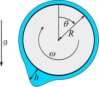
Figure 1: (Color online) Sketch of a drop of a partially wetting liquid coexisting with a thin wetting layer on a rotating cylinder.

The evolution equation for $h(\theta,t)$ is derived employing a long-wave approximation that is valid in the limit $\epsilon\rightarrow 0$, where $\epsilon=\bar{h}/R$ is the ratio between the mean film thickness, $\bar{h}$, and the radius of the cylinder. Also, it is necessary to assume slow variations in the film thickness in the angular direction and small contact angles. With time scale $3\eta R^{4}/\sigma\bar{h}^{3}$, film thickness scale $\bar{h}$ and the angle $\theta$ measured in radians, the non-dimensionalized time-evolution equation is the partial differential equation (PDE) Thiele (2011)

$$\partial_{t}h=-\partial_{\theta}\left\{h^{3}\partial_{\theta}\left[\partial_{\theta}^{2}h+h-B\cos\theta+\Pi(h)\right]+\Omega h\right\},$$ (1)

where $B$ and $\Omega$ are the Bond and rotation numbers defined by

$$B=\frac{R^{2}\rho g}{\epsilon\sigma},\quad\Omega=\frac{\eta\omega R}{\epsilon^{3}\sigma},$$ (2)

respectively. $\Pi(h)$ is the Derjaguin (disjoining) pressure de Gennes (1985); Starov and Velarde (2009); Israelachvili (2011) that here combines long-range attraction and short-range repulsion in the form of power laws Pismen (2001); Pismen and Thiele (2006):

$$\Pi(h)=\frac{H}{h^{3}}\left(1-\frac{b}{h^{3}}\right),$$ (3)

where $H$ is a non-dimensional Hamaker constant. We obtain adequate values of $H$ and $b$ for this form of $\Pi(h)$ by relating them to the (non-dimensional) thickness of the equilibrium wetting layer $h_{0}$ and the static macroscopic equilibrium contact angle $\beta_{0}$:

$$b=h_{0}^{3},\quad H=-\frac{5}{3}\,\beta_{0}^{2}\,h_{0}^{2}.$$ (4)

Note, that $\beta_{0}$ is the angle in the long-wave scaling, i.e., the small physical equilibrium contact angle $\beta_{eq}=\epsilon\beta_{0}$ corresponds to the long-wave equilibrium contact angle $\beta_{0}$ of $O(1)$.

The system is $2\pi$-periodic in $\theta$, and the scaling fixes the non-dimensional mean film thickness to be $1$. Consequently, to leading order in $\epsilon$, the volume of the film per unit length of the cylinder becomes $\int^{2\pi}_{0}h(\theta,t)\,d\theta=2\pi$.

Note that the employed scaling introduced in Ref. Thiele, 2011 allows one, in contrast to scalings used elsewhere in the literature, to directly relate individual dimensionless parameters to important physical parameters. Namely, the rotation number $\Omega$ is proportional to the main experimental control parameter, the angular velocity of the cylinder, that does not enter any other parameter or scale. The ratio of gravity and surface tension enters only the Bond number $B$ (and the overall time scale). The wettability properties control the dimensionless numbers contained in the Derjaguin pressure, Eq. (3). Therefore, the scaling allows one to clearly identify transitions of behavior due to changes in the rotation speed or due to changes in the wetting behavior.

II.2 Numerical methods

We use three different numerical approaches [(i)-(iii)] to analyze this system.

(i) With the first approach, we determine steady thickness profiles (steady-state solutions) employing continuation (or path following) techniques Kuznetsov (2010); Dijkstra et al. (2014). By setting the time derivative in Eq. (1) to zero, we obtain a fourth-order ordinary differential equation (ODE) for the steady film thickness profile $h(\theta)$:

$$-\partial_{\theta}\left\{h^{3}\partial_{\theta}\left[\partial_{\theta}^{2}h+h-B\cos\theta+\Pi(h)\right]+\Omega h\right\}=0.$$ (5)

We then integrate this equation once and use the substitutions $u_{1}=h$, $u_{2}=\partial_{\theta}h$, $u_{3}=\partial_{\theta}^{2}h$ and $u_{4}=\theta$ to transform the equation into an autonomous system of four first-order ODEs:

$$\left\{\begin{array}[]{l}\partial_{\theta}u_{1}=u_{2},\\ \partial_{\theta}u_{2}=u_{3},\\ \displaystyle\partial_{\theta}u_{3}=-u_{2}-B\sin(u_{4})-\Pi^{\prime}(u_{1})\,u_{2}+\frac{c-\Omega u_{1}}{u_{1}^{3}},\\ \partial_{\theta}u_{4}=1,\end{array}\right.$$ (6)

where $c$ is the integration constant that represents the flux. Equations (6) with periodic BCs for $u_{1}$, $u_{2}$, $u_{3}$ and an initial condition for $u_{4}$ are solved numerically by continuation using the continuation and bifurcation software package Auto07p Doedel, Keller, and Kernevez (1991); Doedel and Oldeman (2009). In the context of thin film equations, a similar approach is taken for sliding drops Thiele et al. (2001); Pismen and Thiele (2006), drawn films Tseluiko, Galvagno, and Thiele (2014), self-similar solutions related to film rupture Tseluiko, Baxter, and Thiele (2013), and for steady drops in heterogeneous systems under lateral driving Thiele and Knobloch (2006c). A review is given by Dijkstra et al. Dijkstra et al. (2014) and selected tutorials can be obtained at Thiele et al. Thiele, Kamps, and Gurevich (2014).

(ii) Another way of looking at the problem is by treating PDE (1) as an infinite-dimensional system of ODEs. Then, steady states and time-periodic states of the PDE can be obtained as fixed points and periodic orbits of finite-dimensional systems of ODEs that approximate the infinite-dimensional one. The time-periodic solutions correspond to film-thickness profiles of surface waves or, more importantly, of drops that rotate at their own speed with the cylinder (perform a stick-slip motion). Here, we take advantage of the periodicity and express the solution in the form of the Fourier series with time-dependent coefficients, i.e., $\displaystyle h(\theta,t)=\sum^{\infty}_{k=-\infty}\hat{h}_{k}(t)\,e^{ik\theta}$. Equation (1) can be rewritten as a system of ODEs for the Fourier coefficients, $\hat{h}_{k}$, $k\in\mathbb{Z}$:

$$\frac{d\hat{h}_{k}}{dt}=F_{k}(\hat{h}_{j}),$$ (7)

where $F_{k}$ is a nonlinear function of all the Fourier modes $\hat{h}_{j}$, $j\in\mathbb{Z}$. In practice, we truncate the number of the Fourier modes by restricting $-N\leq k\leq N$ and solve the finite-dimensional system, where $N$ is a large enough integer. Alternatively, finite differences may be used for the spatial discretization, for instance, for settings without periodic BCs Köpf and Thiele (2014). The parameter space of the obtained finite-dimensional ODEs may then be explored with standard continuation techniques Kuznetsov (2010); Dijkstra et al. (2014). Here we employ Auto07p Doedel, Keller, and Kernevez (1991); Doedel and Oldeman (2009). The time-periodic solutions are obtained by first detecting Hopf-bifurcation points on the branches of steady drop profiles and then switching at these points to branches of time-periodic solutions that bifurcate at the Hopf bifurcations. We note that the time period is found as part of the solution, and we do not impose any relation between this period and the period of cylinder rotation. Earlier, the technique based on obtaining a dynamical system for the Fourier coefficients was applied to the continuation of spiral waves in reaction-diffusion systems Bordyugov and Engel (2007). The continuation of Fourier amplitudes can also be employed to follow steady and time-periodic solutions of certain integro-differential equations as recently done in the context of dynamical density functional theory (DDFT) for coarsening Pototsky, Thiele, and Archer (2014) and transport processes Pototsky et al. (2011) of interacting particles in nanopores. The Acknowledgement sketches the recent history of the application of the technique.

(iii) The third approach is to directly integrate the PDE, Eq. (1), in time to obtain time-dependent solutions. We implement a Fourier pseudo-spectral method where spatial derivatives are computed spectrally and time differentiation is performed using a second-order implicit discretization. The resulting nonlinear system is solved by Newton’s method at each time step until convergence is achieved. In this way, we obtain the time evolution for given initial conditions and approach steady and time-periodic states (or other more complicated behavior, such as solutions that are quasi-periodic in time). Note however, that only stable solutions can persist for long time and can be captured by the time-integration method. Unstable solutions are important transient states that will die out in finite time. They can only be captured by continuation techniques that are therefore indispensable if a full understanding of the drop and film hydrodynamics shall be achieved that is encoded in the bifurcation structure of the problem.

We characterize steady-state and time-periodic thickness profiles by the $L^{2}$-norm and the time-averaged $L^{2}$-norm of the difference between the thickness profile and the flat film solution:

$$\|\delta h(\theta)\|\equiv\sqrt{\frac{1}{2\pi}\int^{2\pi}_{0}(h(\theta)-1)^{2}d\theta}$$ (8)

and

$$\|\delta h(\theta,t)\|\equiv\sqrt{\frac{1}{2\pi T}\int^{T}_{0}\int^{2\pi}_{0}(h(\theta,t)-1)^{2}d\theta dt},$$ (9)

respectively. Here, $T$ denotes the time period.

We note that, to ensure accuracy of the results presented in our study, for each of the calculations, we double the number of Fourier modes until convergence is achieved and the results do not change on the scale of the corresponding figure. Besides, we also implement a zero-padding technique to remove aliasing errors. In general, we find that taking $N=64$ is sufficient to ensure accuracy of the computations.

II.3 Parameters

We give a brief overview of the parameters used in Ref. Thiele, 2011, since here we investigate how wettability influences the basic depinning behavior discussed there. Estimates for realistic Bond and rotation numbers are based on two liquids typically studied in the literature: (i) water at $25^{\circ}$C with $\sigma=0.072$N/m, $\eta=0.001$kg/ms and $\rho=1000$kg/m³ as in Reisfeld et al. Reisfeld and Bankoff (1992) and a silicone oil with $\sigma=0.021$N/m, $\eta=1$kg/ms and $\rho=1200$kg/m³ as in Evans et al. Evans, Schwartz, and Roy (2004). As experimentally feasible configurations, we assume angular rotation velocities $\omega=0.1$–$10$ s^-1, cylinders of radii $R=10^{-3}$–$10^{-2}$ m and smallness ratios $\varepsilon=0.01$–$0.1$.

For $\omega=1$ s^-1, the smallness ratio $\varepsilon=0.1$ and the cylinder radius of $R=10^{-3}$m, we find for case (i) $B=1.36$ and $\Omega=0.014$, whereas for case (ii) $B=5.61$ and $\Omega=47.6$. Increasing the cylinder radius to $R=10^{-2}$ m, increases all the Bond numbers by a factor $10^{2}$ and all the rotation numbers by a factor $10$, whereas, decreasing the smallness ratio to $\varepsilon=10^{-2}$, increases all the Bond numbers by a factor $10$ and all the rotation numbers by a factor $10^{3}$. Therefore, focusing on cylinder diameters in the millimeter range, we mainly investigate $B\leq 10$, although the structure of steady-state solutions for higher Bond numbers is discussed. The rotation number can be widely varied, although we find that for $B=O(1)$, the interesting range for the rotation number is $\Omega=O(1)$. For instance, with $B=1$, one finds that depinning occurs at $\Omega\approx 1.68$.

II.4 The aims of the present study

The preliminary work in Ref. Thiele, 2011 introduces the model incorporating wettability and studies a single partially wetting case at the equilibrium contact angle $\beta_{0}=2$ that is rather large in the long-wave scaling. In particular, bifurcation diagrams are discussed for steady profiles as functions of the Bond number and for steady pinned states and time-periodic depinned drops as functions of the rotation number. One particular depinning transition – the Saddle-Node-Infinite-PERiod (or SNIPER) bifurcation Strogatz (1994) – is introduced. This is contrasted with some basic results for the completely wetting case ($\beta_{0}=0$). As the focus of Ref. Thiele, 2011 was on the main depinning transition, they only employed continuation to obtain branches of steady drops and film solutions directly connected to the stable pendent drop solution at low rotation speed or to the film solution at large rotation speed. In the case without rotation, the focus was on single-drop solutions. In consequence, the results of Ref. Thiele, 2011 represent only a first glimpse at the system and turn out to be rather incomplete. We show here that the complete bifurcation diagrams are much richer even in the case without rotation, not to speak of the case with driving where we now discuss several branches of time-periodic solutions.

The present work investigates both steady and time-periodic states in more detail. First, this shall result in a deeper understanding of the case with $\beta_{0}=2$ studied in Ref. Thiele, 2011. The second and more important part of the present study analyzes how the bifurcation behavior (the depinning transition) changes as the wettability is changed. In other words, we investigate how the complex bifurcation structure found at large contact angles emerges from the rather trivial behavior at zero contact angle. This is done through the consideration of several intermediate cases with $0<\beta_{0}<2$.

The present detailed study of the depinning transition and its transformations shall also establish the present system, the hydrodynamic system of a rotating cylinder covered by a partially wetting liquid, as a reference system for depinning transitions in other hydrodynamic systems, more general soft matter systems and beyond. Such systems are characterized by a spatial heterogeneity (here, the inhomogeneity in the action of gravity along the cylinder circumference), a lateral driving (here, the rotation of the cylinder) and a cohesive force resulting in coherent structures (here, partial wettability resulting in coherent drops). A weakening of the cohesive force (here, increasing wettability, i.e., approaching the wetting transition) will change the depinning transition in all such systems and the present study shall reveal possible corresponding pathways in the system behavior.

Throughout this study, we focus on positive values of the rotation number and the Bond number, but we may also exploit the fact that all the obtained bifurcation diagrams are symmetric about the respective zero values of these two parameters, since a reflection in $\Omega$ corresponds to turning the cylinder in the anti-clockwise direction and a reflection in $B$ stands for reversing the direction of gravity. Therefore, it is perfectly acceptable to reflect solution branches at the axes of the Bond and rotation numbers, providing a useful technique for reducing the number of computations needed to obtain a full set of solution branches through path following. We also fix the thickness of the wetting layer to be $h_{0}=0.1$ when exploring the other parameters.

III Steady-state film and drop profiles

III.1 Steady states in the partially wetting case

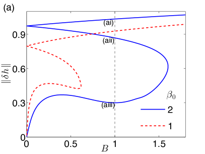
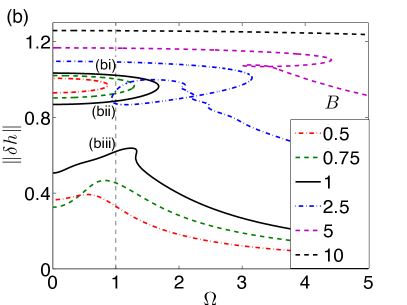
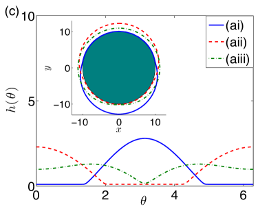
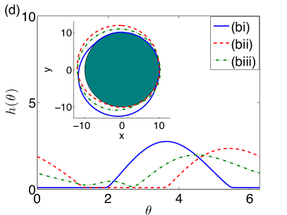
Figure 2: (Color online) (a) Branches of steady drop solutions on a horizontal cylinder without rotation ($\Omega=0$) for various equilibrium contact angles $\beta_{0}$ characterized by their $L^{2}$-norm as functions of the Bond number. The dashed vertical line corresponds to $B=1$, and the thickness profiles $h(\theta)$ corresponding to points (ai)–(aiii) at $\beta_{0}=2$ are shown in panel (c) with the inset giving the profiles on a cylinder assuming a radius $R=10$. (b) Branches of steady drop solutions on a horizontal rotating cylinder for $\beta_{0}=2$ as functions of the rotation number $\Omega$ for various Bond numbers $B$ as given in the legend. The dashed vertical line corresponds to $\Omega=1$, and the thickness profiles corresponding to points (bi)–(biii) at $B=1$ are shown in panel (d) with the inset giving the profiles on a cylinder assuming a radius $R=10$. The curves in panels (a) and (b) agree with Figs. 2 and 4 of Ref. Thiele, 2011, respectively. However, here they are calculated with numerical methods (i) and (ii) (see Sec. II.2) that perfectly agree on the presented scale. This also serves as a validation of the novel method (ii).

First, we consider steady drop and film solutions on the resting cylinder, i.e., at $\Omega=0$, for the two particular values $\beta_{0}=1$ and $2$ of the equilibrium contact angle that correspond to partial wetting. Changing the Bond number, $B$, we obtain families of steady-state solutions as displayed in Fig. 2(a). One observes that the layout of the branches (the bifurcation structure) is very similar in the two cases, only the size of the structure is smaller for smaller $\beta_{0}$. Without gravity ($B=0$) there are only two solutions: an unstable flat film (the $L^{2}$-norm, defined by Eq. (8), is zero) and a stable drop solution (the $L^{2}$-norm is slightly smaller than one) that is invariant with respect to translation in $\theta$ as for $B=0$ the system is homogeneous. Once $B>0$, only two positions survive and two individual branches emerge from the drop solution at $B=0$ that correspond to unstable drops sitting symmetrically on top of the cylinder (smaller $L^{2}$-norm) and to stable pendent drops hanging symmetrically beneath the cylinder (larger $L^{2}$-norm), respectively. The unstable flat film also becomes modulated for $B>0$. In consequence, for small $B$, three steady profiles exist which correspond to different distributions of the liquid on the cylinder. The three profiles on the dashed vertical line corresponding to points (ai)–(aiii) in Fig. 2(a) ($\beta_{0}=2$ and $B=1$) can be found in Fig. 3 of Ref. Thiele, 2011 and are also shown in Fig. 2(c) with the inset giving the profiles on a cylinder assuming a radius $R=10$. Above a critical $B=B_{\mathrm{sn}}$, only the stable pendent drop remains while the other two solutions annihilate at $B_{\mathrm{sn}}$ in a saddle-node (SN) bifurcation. $B_{\mathrm{sn}}$ monotonically increases with the contact angle $\beta_{0}$, e.g., it reaches the value $B\approx 43.3$ for $\beta_{0}=10$. We note that a pendent drop exists at any $B$ in the employed long-wave framework. However, at large $B$ the long-wave approximation itself becomes invalid. A full hydrodynamic description then shows drops that drip off the cylinder Hazel (2014).

Next, we discuss the changes in the observed steady profiles when the cylinder is rotated. We increase the rotation number $\Omega$ from zero and obtain solution branches as shown in Fig. 2(b) for various Bond numbers and $\beta_{0}=2$. First, we consider the case $B=1$ (solid black lines) and note that although one finds 3 solutions for $\Omega=0$ as expected from the crossings of the dashed line and the $\beta_{0}=2$ curves in Fig. 2(a), a close inspection shows that the solutions of the smallest $L^{2}$-norms do actually not correspond to each other. This mismatch that was already pointed out in Ref. Thiele, 2011 indicates that the branch structures in Fig. 2 are not complete (see the discussion in Sec. II.4). It will be completed below after discussing Fig. 2(b). The vertical dashed line in Fig. 2(b) corresponds to $\Omega=1$ and the profiles (bi)–(biii) for $B=1$ are shown in Fig. 2(d).

Increasing $\Omega$ from zero, the stable pendent drop (top branch in Fig. 2(b)) is shifted towards the left-hand side of the cylinder, i.e., towards larger $\theta$. Furthermore, the drop widens marginally, thereby decreasing its $L^{2}$-norm. This branch annihilates with the closest unstable branch (drops on top of the cylinder) in an SN bifurcation at $\Omega_{\mathrm{sn}}\approx 1.68$ where a depinning transition occurs Thiele (2011). For $\Omega>\Omega_{\mathrm{sn}}$ the drop overcomes the downward pull of gravity, due to the frictional forces exerted by the rotating cylinder. As a result, the solution becomes time-periodic and the drops move around the cylinder with a position-dependent velocity. For space-time plots, see Fig. 7 of Ref. Thiele, 2011.

Close to the depinning transition, the difference in the time scales of slow and fast phases diverges and the drop motion strongly resembles stick-slip motion as also discussed in the context of drop motion on heterogeneous substrates Thiele and Knobloch (2006b). The square-root dependence of the frequency $1/T$ of the drop motion with time period $T$ on the driving $\Omega-\Omega_{\mathrm{sn}}$ indicates that at $\Omega_{\mathrm{sn}}$ one has a SNIPER bifurcation.

The mismatch observed above indicates that at $\Omega=0$ Figs. 2(a) and (b) miss at least a steady solution with an $L^{2}$-norm of $0.5$ and $0.3$, respectively. The starting point of our present analysis is a continuation of the steady profiles that are not consistent between the figures in the respective required parameter. Note that this alone does not necessarily provide a complete set of solutions since it is possible that further solutions exist that are not connected in this way to the already known solutions. Therefore, we also perform two-parameter continuations of the loci of the observed SN bifurcations (fold continuation), starting at several values of $B$ and continually check the consistency between the figures. Once all the figures are consistent, all the steady solution branches should be present in the studied range of parameters.

First, we expand in Fig. 3(a) the results of Fig. 2(b) for intermediate values $B=1.25$, $1.5$ and $2$ and notice that there exists a rather complex structure involving multiple solutions in an intermediate $\Omega$-range: for $B=1.25$ there are three separate curves that for $B=1.5$ merge into $2$ curves and then for $B=2$ into a single-loop structure.

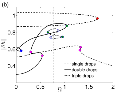
Figure 3: (Color online) (a) Extension of Fig. 2(b) for intermediate Bond numbers displaying the complex structure of the branches that involve several SN bifurcations. (b) Extension of Fig. 2(b) for $B=1$ and $\beta_{0}=2$, representing the steady solutions already present in Fig. 2 as dashed lines (stable/unstable single drops and films) and the additionally determined solutions as the solid lines (unstable double drops) and dot-dashed lines (unstable triple drops). Saddle-node bifurcations (folds) are marked with solid circles with colors corresponding to the respective fold-continuation curves in Fig. 4. Profiles for solutions on the vertical thin dashed line that corresponds to $\Omega=0.767$ are shown in Fig. 5.

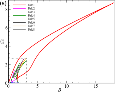
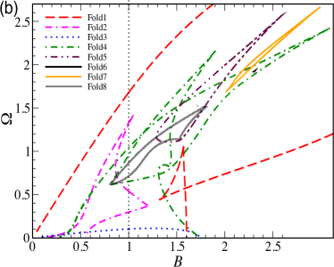
Figure 4: (Color online) Shown are the loci of saddle-node bifurcations in the ($B,\Omega$)-plane for $\beta_{0}=2$. Panel (a) gives a complete view while panel (b) gives a zoom into the region where most folds are located. The vertical thin dotted line indicates the case $B=1$ that is consistent with Fig. 3(b) showing eleven folds with corresponding line colors.

To investigate the reconnections and the related additional branches, we continue the loci of all encountered SN bifurcations in the ($B,\Omega$)-plane. This includes codimension-two bifurcations where pairs of SN bifurcations are created/annihilated. The three observed processes are a hysteresis bifurcation, the destruction/creation of an isola of solutions and a necking bifurcation (cf., e.g., Thiele et al. Thiele and Knobloch (2004)). The resulting full fold-tracking diagram shown in Fig. 4(a) with a zoom into the most relevant region in Fig. 4(b) determines the folds that exist for any given Bond number. For example, at $B=1$, eleven folds at particular $\Omega$ are found, yet, Fig. 2(b) only displayed three. Selecting the “new” folds, one may again employ continuation in $\Omega$ to obtain the complete bifurcation diagram of steady profiles in Fig. 3(b).

We observe that around $\Omega=0.8$ there exists a “figure-eight” isola of solutions. What makes these solutions particularly interesting is that they are not related to any equilibrium solutions that may exist at $\Omega=0$ for otherwise the same parameters. In particular, the solutions correspond to unstable triple-drop/hump solutions, that for $B=1$ and $\beta_{0}=2$ do not exist without rotation, i.e., without non-equilbrium driving. In other words, a finite driving brings into existence solutions expected at other parameter values. Typical single-, double- and triple-drop profiles located on the vertical dotted line in Fig. 3(b) are illustrated in Fig. 5. As expected, all the profiles are off center, i.e., rotation drags profiles towards the left-hand side of the cylinder. Although all double- and triple-drop solutions are unstable, their understanding is crucial for the understanding of the behavior of the hydrodynamic system: they provide the phase space of the system with a rich structure that allows for complex dynamical states (see Sec. IV).

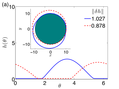
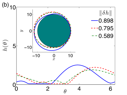
Figure 5: (Color online) Steady drop profiles on a horizontal cylinder for $\Omega=0.767$, $\beta_{0}=2$ and $B=1$, i.e., at the loci indicated by the vertical thin dashed line in Fig. 3(b). The individual panels give (a) single-, (b) double- and (c) triple-drop solutions, with the $L^{2}$-norms $\|\delta h\|$ as given in the legends. The insets show the profiles on a cylinder assuming a radius $R=10$.

The remaining part of the new structure in Fig. 3(b) intersects $\Omega=0$ four times, with the $L^{2}$-norms $\|\delta h\|\approx 0.30$, $0.62$ and a double intersection at $0.59$. This indicates that an entire system of branches is missing in Fig. 2(b) showing the equilibrium case. The solution with the $L^{2}$-norm $0.30$ is the solution missing in Fig. 2(b). As the additionally encountered branches cross $\Omega=0$, also the system of equilibrium profiles needs completion. This is achieved through continuation in $B$ at $\Omega=0$.

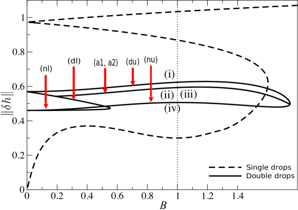
Figure 6: (Color online) Branches of steady profiles for $\beta_{0}=2$. The $L^{2}$-norms are given as functions of the Bond number $B$. The dashed lines represent single-drop solutions also present in Fig. 2(a) while the solid lines give the bifurcation structure of unstable double-drop solutions. There we distinguish symmetric drop (d$\mathrm{u}$, d$\mathrm{l}$) and nucleation or hole (n$\mathrm{u}$, n$\mathrm{l}$) and asymetric (a$\mathrm{1}$, a$\mathrm{2}$) solutions. Subscripts “u” and “l” refer to the respective upper and lower solution. The profiles at $B=1$ (indicated by the vertical dotted line and marked by (i)–(iv)) are displayed in Fig. 7. We also note that only the branch that corresponds to pendent drop solutions is stable (the branch with the largest $L^{2}$-norms). All the other branches are unstable.

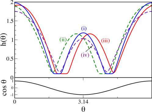
Figure 7: (Color online) Selected profiles of steady unstable double-drop solutions on a horizontal cylinder, without rotation ($\Omega=0$), at $B=1$ and $\beta_{0}=2$ corresponding in Fig. 6 to the crossing points of the vertical dotted line and the solid lines (with the labels (i)–(iv)). They present examples of profiles from branches d$\mathrm{u}$, a$\mathrm{1}$, a$\mathrm{2}$ and n$\mathrm{u}$, respectively. The symmetries are discussed in the main text.

All the resulting solutions corresponding to unstable double-drop solutions are included in Fig. 6 as solid black lines. The profiles indicated at $B=1$ by the vertical dotted line and marked by (i)–(iv) are displayed in Fig. 7. As they also correspond to the $\Omega=0$ states in Fig. 3(b), we deduce that the central line in Fig. 6 is actually a double branch since in Fig. 3(b) two branches meet at $\Omega=0$, with the $L^{2}$-norm of $0.59$. As these are the only branches in Fig. 3(b) which do not have zero slope at $\Omega=0$, they correspond to the two mirror images with respect to $\theta=\pi$ of an asymmetric solution [profiles (ii) and (iii) in Fig. 7]. We name these branches a$\mathrm{1}$ and a$\mathrm{2}$ (where ‘a’ refers to ‘asymmetric’). They emerge at pitchfork bifurcations from the other branches that correspond to drop and hole (or nucleation) solutions that are themselves symmetric with respect to reflection at $\theta=\pi$. We name them d$\mathrm{u}$, d$\mathrm{l}$, n$\mathrm{u}$, and n$\mathrm{l}$ (where ‘d’ and ‘n’ refer to ‘drop’ and ‘nucleation’, respectively, and ‘u’ and ‘l’ refer to respective upper and lower solutions), see Fig. 6. Figure 7 gives examples for d$\mathrm{u}$ and n$\mathrm{u}$ solutions, see profiles (i) and (iv), respectively. For the d$\mathrm{u}$ and n$\mathrm{u}$ solutions shown in Fig. 7, there is one large drop on top of the cylinder and another smaller one underneath. In contrast, the d$\mathrm{l}$ and n$\mathrm{l}$ branches consist of profiles where the two holes are on top and underneath of the cylinder (not shown).

Note, that the unstable double-drop solutions exist at larger Bond numbers than the unstable single-drop solutions and may, therefore, influence the dynamics up to larger values of $B$. Yet, as before, above a critical value ($B\approx 1.749$), only the stable pendent drop remains.

To understand why Fig. 6 has the two double-drop solutions at $\Omega=0$ and $B=0$ that give rise to the entire double-drop branch structure at $B>0$ even without driving, we consider in Appendix A.1 the case $\Omega=0$, $B=0$ in an extended parameter space. Also, Appendix A.2 gives some further details of the behavior of the double-drop solutions of Fig. 6.

III.2 Transition to the completely wetting case

The rich solution structure at equilibrium ($\Omega=0$) and, in consequence, out of equilibrium ($\Omega>0$) is mainly due to partial wettability. This implies that most of this structure has to disappear when wettability is increased, i.e., when the equilibrium contact angle $\beta_{0}$ is decreased. Before we move on to the full bifurcation structure including time-periodic thickness profiles, here, we briefly emphasize the contrasting structure of steady profiles found for completely wetting liquids, when $\beta_{0}$ approaches zero. As observed in Fig. 2(a), for a resting horizontal cylinder without rotation the critical Bond number $B_{\mathrm{sn}}$ where the two unstable drop solutions annihilate, i.e., where a qualitative transition occurs, decreases with $\beta_{0}$. In parallel, the modulated film transforms into a pendent drop that is at $\beta_{0}=0$ the only solution for any non-zero Bond number.

For a completely wetting liquid, there exists no force beside gravity that favors drops as opposed to a flat film. Gravity can still produce pendent drops. However, for non-zero Bond numbers at $\Omega=0$, the model, Eq. (1), does not have continuous $2\pi$-periodic steady-state solutions, but only solutions with a finite support, i.e., pendent drops on a dry substrate. They can be studied employing a weak formulation. See Appendix B.1 and Refs. Reisfeld and Bankoff, 1992; Evans, Schwartz, and Roy, 2004 for further details.

Then for $\Omega>0$, continuous $2\pi$-periodic steady solutions exist as the lateral driving creates a dynamic wetting layer. Increasing $\Omega$, the droplets change monotonically, the rotation shifts them towards the left and smears them out at the same time. Figure 8(a) gives for various $B$ the main branch structure as a function of $\Omega$ for a partially wetting liquid of a smaller contact angle $\beta_{0}=1$ while Fig. 8(b) gives this structure close to complete wetting at $\beta_{0}=0.1$.

From Fig. 2(b) to Fig. 8(a), and further to Fig. 8(b), one observes a clear transition towards a much simpler branch structure as the contact angle $\beta_{0}$ decreases. Actually, all complex aspects of branch patterns discussed at Figs. 2(b) and 3 disappear resulting, e.g., at $\beta_{0}=0.1$, in a rather simple branch of steady solutions with a monotonically decreasing $L^{2}$-norm. In particular, as the contact angle is decreased, all the SN bifurcations occurring for various values of the rotation and Bond numbers (cf. Fig. 4) are eliminated in various codimension-two bifurcations. Thereby, the prominent SN bifurcation, that at $\beta_{0}=2$ is related to the SNIPER bifurcation, is the bifurcation structure that exists for the largest range of $\beta_{0}$. It is a particularly intriguing question what happens to the SNIPER bifurcation and the emerging branch of time-periodic solutions (stick-slipping drops) when the wettability increases, i.e., $\beta_{0}$ decreases. This is studied in Sec. IV.

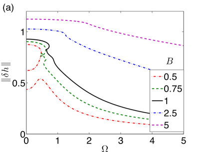
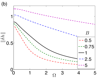
Figure 8: (Color online) Shown are branches of steady states for different Bond numbers $B$ (as given in the legends) as functions of the rotation number $\Omega$ for equilibrium contact angles (a) $\beta_{0}=1$ and (b) $\beta_{0}=0.1$.

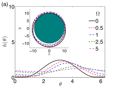
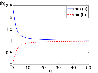
Figure 9: (Color online) (a) Steady film-thickness profiles for the approximate case of complete wetting ($\beta_{0}=0.1$) with $B=1$ for several rotation numbers. (b) The maximum (blue solid line) and minimum (red dashed line) of the steady film thickness showing that the profile tends to a flat film with increasing $\Omega$.

The case of the smallest considered contact angle $\beta_{0}=0.1$ is already close to the complete wetting case. Selected steady drop profiles that correspond to the solution branch for $B=1$ in Fig. 8(b) are displayed in Fig. 9(a). For increasing $\Omega$, the driving drags the liquid along the surface of the cylinder, resulting in a steady drop whose center of mass moves towards a larger $\theta$. However, as wettability is large, the adhesion force that keeps the drop together is weak and the drop can now deform strongly. The drop becomes shallow as indicated by the monotonically decreasing/increasing maximum/minimum values of its profile, as shown in Fig. 9(b). Finally, at large $\Omega$, it approaches a flat-film solution. In other words, the drop does not survive as a “coherent structure” due to the attenuated influence of partial wettability. We notice that the drops flatten and smear out well before their maxima reach $\theta=3\pi/2$ (the left-hand-side of the cylinder), where gravity becomes tangential to the cylinder surface.

IV Branches of time-periodic flow states

To better understand the behavior of the system, one also needs to obtain the branches of unsteady flows, i.e., time-periodic film and drop profiles as, e.g., co-rotating drops on the cylinder or surface waves. Another point to clarify is how the time-periodic states emerge from the already discussed branches of steady profiles. Ref. Thiele, 2011 only considered the large contact angle case $\beta_{0}=2$ and obtained a single time-periodic solution branch for $\Omega>\Omega_{\mathrm{sn}}$ using direct numerical time integration. This method allows one to establish that the main depinning transition for the partially wetting drop on a rotating cylinder is a SNIPER bifurcation similar to the case of a drop on a heterogeneous substrate Thiele and Knobloch (2006b). However, as the direct numerical simulation follows the evolution in time starting from an initial condition, it does not allow for a determination of unstable steady or time-periodic states. As these are needed to develop a full understanding of the involved qualitative transitions, in the current study, we obtain both, stable and unstable states, via numerical continuation as outlined above in Sec. II. In what follows, we fix the Bond number, $B=1$, and investigate the changes of the bifurcation diagram when the equilibrium contact angle $\beta_{0}$ varies.

IV.1 The case of a large contact angle ($\beta_{0}=2$)

We start with the case of a “large” contact angle ($\beta_{0}=2$). The complete bifurcation diagram is presented in Fig. 10 where panel (a) gives the solution measure $\|\delta h\|$, defined by the $L^{2}$-norm in Eq. (8) for steady-state profiles and by the time-averaged $L^{2}$-norm in Eq. (9) for time-periodic flow states, as a function of the rotation number over the full range, while panel (b) presents a zoom into the region of small values of $\Omega$. Steady-state solution branches are shown as (blue) solid lines while the time-periodic solution branches are given as (red) dashed lines. In this figure and in the figures that follow, stable/unstable branches of steady-state solutions are indicated by “S” and “U”, respectively, and stable/unstable branches of time-periodic solutions are indicated by “s” and “u”, respectively. Furthermore, the loci of Hopf bifurcations (HBs), homoclinic bifurcations (HCs) and SNIPER bifurcations are indicated by circles, squares and stars, respectively. In total, there exist four HBs, two HCs, one SNIPER and five time-periodic solution branches.

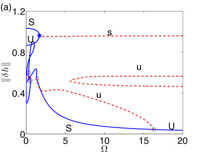
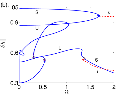
Figure 10: (Color online) The complete bifurcation diagrams for $\beta_{0}=2$ and $B=1$ giving the solution measure $\|\delta h\|$ in dependence on the rotation number $\Omega$. It includes the steady profiles (blue solid lines) and time-periodic profiles (red dashed lines). The HBs are indicated by circles, the HCs are indicated by squares and the SNIPER is indicated by a star. (a) The complete bifurcation diagram. (b) A zoom of panel (a) into the small-$\Omega$ region where most of the bifurcation structure is located. The stabilities of the states are discussed in the main text.

It is found that steady-state solutions exist for all rotation numbers. In particular, for large enough $\Omega$, the solution measure of the steady-state solution decreases as $\Omega$ increases, and we find that the solution approaches the uniform coating state $h\equiv 1$. See Appendix B.2.1 for further details. Besides, below [above] the value $\Omega\approx 16.4$ at which the rightmost HB exists, steady-state solutions are linearly stable [unstable]. At this HB, a branch of unstable time-periodic solutions emerges subcritically. As can be seen in Fig. 10(a), the solution measure of the time-periodic solution increases as $\Omega$ decreases and the branch terminates at another HB at $\Omega\approx 1.37$.

The only branch of stable time-periodic solutions emerges in a SNIPER at the SN of the steady-state branch at $\Omega_{\mathrm{sn}}\approx 1.68$. This SNIPER was found using numerical time integration in Ref. Thiele, 2011. In the limit $\Omega\rightarrow\infty$ along this branch, the solution is equivalent to a drop solution at zero Bond number that co-rotates with the cylinder. A corresponding detailed asymptotic analysis is presented in Appendix B.2.2. We note that there is one more branch of time-periodic solutions that is not connected to any of the branches of steady-state solutions. It has an SN at $\Omega\approx 5.64$, and both the upper and lower parts of this branch extend to infinitely large values of $\Omega$. In the limit $\Omega\rightarrow\infty$ along the upper and lower parts of this branch, the solutions are equivalent to double-drop solutions at zero Bond number that co-rotate with the cylinder. We note that both the upper and lower parts of this branch are linearly unstable.

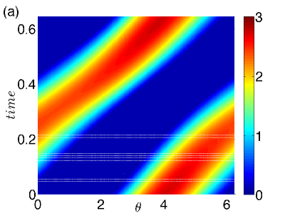
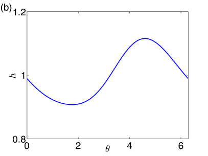
Figure 11: (Color online) An example of multistability: Two solutions that are stable at the identical parameter values, $\Omega=10$, $\beta_{0}=2$ and $B=1$. Panel (a) shows the space-time contour plot of the stable time-periodic profile, while panel (b) shows the stable steady profile.

The bifurcation diagram in Fig. 10(a) suggest that extended ranges of multistability exist, i.e., depending on initial conditions, time simulations will show different long-time solutions at a given rotation number. For $1.68<\Omega<16.4$, the stable long-time solution may either be a small-amplitude steady profile or a large-amplitude time-periodic profile. For $\Omega>16.4$, the small-amplitude steady profile is unstable and only the large-amplitude time-periodic profile remains as an attractor. Figure 11 shows as an example the two stable long-time states for $\Omega=10$. The large-amplitude time-periodic profile is shown in the contour-plot in panel (a), while the small-amplitude steady profile is shown in panel (b).

We also note that at each of the HB points at $\Omega\approx 0.31$ and at $\Omega\approx 0.54$ a short branch of unstable time-periodic states emerges that terminates in an HC on a branch of steady profiles.

IV.2 The case of a medium contact angle ($\beta_{0}=1$)

We next investigate the case of a “medium” contact angle ($\beta_{0}=1$). The complete bifurcation diagram is presented in Fig. 12(a). It is found that there exist six HBs and one HC. The rightmost HB is at $\Omega\approx 38.7$ and the other five HBs are clustered around $\Omega\approx 0.8$. Figure 12(b) shows a zoom of this region. Similar to the diagram for $\beta_{0}=2$, steady profiles exist for all rotation numbers. At the HB at $\Omega\approx 38.7$, a branch of unstable time-periodic solutions emerges subcritically. As can be seen in Fig. 12(a), the solution measure of the time-periodic solution increases as $\Omega$ decreases and the branch turns back towards larger $\Omega$ at a saddle-node bifurcation (at $\Omega\approx 2.5$ ) where its stability changes. As $\Omega$ increases again, the solution measure of this stable solution increases as well. In the limit $\Omega\rightarrow\infty$, the solution is equivalent to a drop solution at zero Bond number that co-rotates with the cylinder.

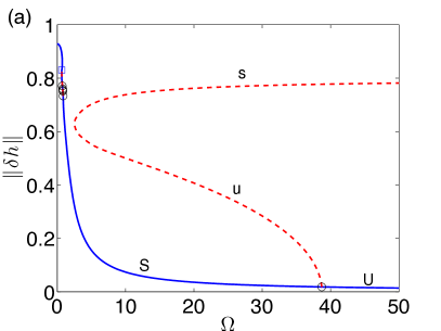
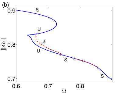
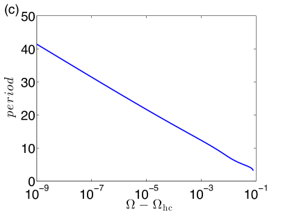
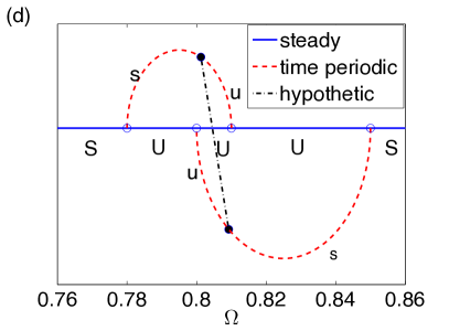
Figure 12: (Color online) (a) The complete bifurcation diagram for $\beta_{0}=1$ and $B=1$ giving the solution measure $\|\delta h\|$ in dependence on the rotation number $\Omega$. It includes the steady and time-periodic states. (b) A zoom of panel (a) into the small-$\Omega$ region where most of the bifurcation structure is located. (c) A plot of the period over the logarithm of $\Omega-\Omega_{\mathrm{hc}}$ for the time-periodic branch originating at $\Omega\approx 0.74$ in panel (b). (d) A schematic representation showing the connection of the four HBs at $\Omega\approx 0.78$, $0.80$, $0.81$ and $0.85$ in panel (b). The HBs are indicated by circles. There exist two time-periodic branches, one of them connects HBs at $0.78$ and $0.81$, and the other one connects HBs at $0.80$ and $0.85$. In addition, on each of the time-periodic branches there exist torus bifurcations that are indicated by filled circles. We expect that there exists a branch of quasi-periodic solutions that connects the two torus bifurcations. This hypothetic branch is schematically represented by the black dot-dashed line, but has not been actually computed while all the other branches and all the bifurcations have been computed.

Next, we analyze the solutions in the range of smaller $\Omega$. For $0\leq\Omega<0.64$, there exits only one solution for each rotation number that is a stable steady-state solution. As $\Omega$ increases, the solution measure of this solution decreases until it reaches an SN at $\Omega\approx 0.73$ where the branch becomes unstable and turns back towards smaller $\Omega$. See, e.g., Fig. 12(b). Following the branch with decreasing $\|\delta h\|$, one passes another SN at $\Omega\approx 0.64$, a second eigenmode becomes unstable and the branch turns again towards larger $\Omega$. Continuing towards larger $\Omega$, one crosses $5$ HBs (at $\Omega\approx 0.74$, $0.78$, $0.80$, $0.81$ and $0.85$). In this region, the steady-state solution is stable only for $0.74<\Omega<0.78$ and for $0.85<\Omega<38.4$. At each HB, a branch of time-periodic solutions emerges. The one that starts supercritically at the first HB at $\Omega\approx 0.74$ is stable and reconnects at $\Omega_{\mathrm{hc}}\approx 0.66$ in a homoclinic global bifurcation to the unstable part of the steady-state branch between the two SNs. This classification as a homoclinic bifurcation is supported by Fig. 12(c), where $\Omega-\Omega_{\mathrm{hc}}$ is plotted against the temporal period in a linear-log plot. The figure shows that the period diverges logarithmically as $\Omega-\Omega_{\mathrm{hc}}$ approaches zero. This is the signature of a homoclinic bifurcation Strogatz (1994) and is also a common scenario for systems where depinning occurs Köpf et al. (2012); Köpf and Thiele (2014); Pailha et al. (2012); Herde et al. (2012).

The HBs at $\Omega\approx 0.78$ and $0.81$ are connected by one time-periodic branch and the HBs at $\Omega\approx 0.80$ and $0.85$ are connected by another time-periodic branch that in part overlaps with the first one. But since the solution measures $\|\delta h\|$ of these time-periodic solutions and the steady-state solutions are very similar to each other for the values of $\Omega$ in this range, the branches are almost indistinguishable in Fig. 12(b). To illustrate the connections, a schematic representation of this region is shown in Fig. 12(d) where also the stabilities are indicated. In addition, on the two time-periodic branches, we detect that the stability of the time-periodic solutions changes, which is an indication of torus bifurcations, at $\Omega\approx 0.802$ and $0.805$, respectively. The fact that the time-periodic solutions undergo torus bifurcations at these values of $\Omega$ is supported by the observation that at these points there exist pairs of complex-conjugate Floquet multipliers crossing the unit circle. Namely, at $\Omega\approx 0.802$ and $0.805$, we find that the multipliers $0.545\pm 0.838\,i$ and $0.155\pm 0.988i$, respectively, cross the unit circle. We expect that there exists a branch of quasi-periodic solutions that connects the two torus bifurcations. However, with the current continuation tools we are not able to continue solutions on this solution branch. We, therefore, draw schematically a (black) dot-dashed line in Fig. 12(d) to connect the two torus bifurcations to indicate the existence of such a stable solution branch, that has not actually been computed by continuation.

With the information presented above, we conclude that the time-periodic solutions are stable in the ranges $0.78<\Omega<0.802$ and $0.805<\Omega<0.85$, which is also verified using numerical time integration of Eq. (1). We choose $\Omega=0.79$ as an example. The initial condition is the state of homogeneous coating, $h(x,0)=1$, and the $L^{2}$-norm of the solution, $\|\delta h\|$, is extracted in the range $400<t<500$, to study the long-time behavior. Figure 13(a) shows the $L^{2}$-norm of the solution, $\|\delta h\|$, versus $t$ and Figure 13(b) shows $\frac{d}{dt}(\|\delta h\|^{2})$ versus $\|\delta h\|^{2}$. It clearly indicates that the solution evolves to a time-periodic solution.

However, in the range $0.802<\Omega<0.805$, i.e., between the two torus bifurcations, no stable steady profiles or single-frequency time-periodic solutions exist. Therefore, it is likely that the attractor corresponds either to a double-frequency time-periodic state or a multi-frequency solution (if further bifurcations of the double-frequency time-periodic state occur in this very small $\Omega$ range). With identical initial conditions as before, at $\Omega=0.804$ a numerical time simulation gives the trajectory presented in Figs. 13(c) and (d) (the $L^{2}$-norm of the solution is extracted in the range $100<t<200$). The results indicate a double-frequency time-periodic state consistent with the hypothesis formulated above. Therefore, we expect that the hypothetical (black) dot-dashed branch in Fig. 12(d) joining the two torus bifurcations is a quasi-periodic solution branch that is at least in part of this $\Omega$-range linearly stable.

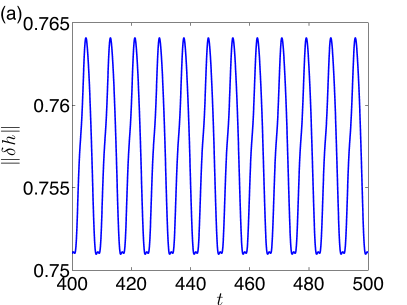
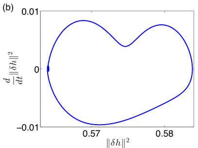
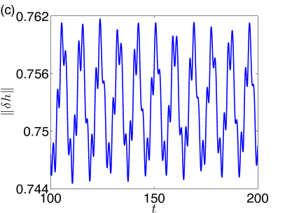
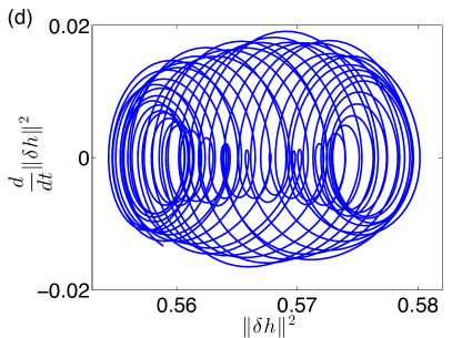
Figure 13: (Color online) Results of the numerical time integration of Eq. (1) for $\beta_{0}=1$, $B=1$ and $\Omega=0.79$ (panels (a) and (b)) and $\Omega=0.804$ (panels (c) and (d)). Panels (a) and (c) show the time evolution of the $L^{2}$-norm, $\|\delta h\|$, for $\Omega=0.79$ and $0.804$, respectively, and panels (b) and (d) show the corresponding curves in the phase plane $(\|\delta h\|^{2},d(\|\delta h\|^{2})/dt)$.

IV.3 Transition from a large ($\beta_{0}=2$) to a medium ($\beta_{0}=1$) contact angle

After having analyzed the diagrams for large and medium contact angles, we next study the transitions in between. Comparing the diagrams for $\beta_{0}=2$ in Fig. 10(a) and $\beta_{0}=1$ in Fig. 12(a), one notices that the two time-periodic branches for $\beta_{0}=2$, where one is the unstable branch connecting the two HBs and the other is the stable branch that emerges in the SNIPER bifurcation, have at $\beta_{0}=1$ somehow merged into one branch that emanates from the HB at $\Omega\approx 38.7$. One should also note that, as a consequence, when a putative hydrodynamic experiment is performed, the observed sequence of behaviors is very different when $\Omega$ is continuously increased for $\beta_{0}=2$ and for $\beta_{0}=1$. For liquids with the large contact angle ($\beta_{0}=2$), a pendent droplet directly evolves into a large-amplitude time-periodic state that represents a droplet co-rotating with the cylinder, while for liquids with the medium contact angle ($\beta_{0}=1$), a pendent droplet first changes into a steady uniform coating film before eventually changing into a large-amplitude time-periodic wave for sufficiently large values of $\Omega$.

In what follows, we will see that the transitions of branches and bifurcations are rather complicated and involve several steps. We focus on the main transitions and show how the bifurcation diagram changes when $\beta_{0}$ is varied and, in particular, how the SNIPER bifurcation disappears.

The bifurcation diagram for $\beta_{0}=1.4$ is shown in Fig. 14, and Fig. 15 shows zooms into the small-$\Omega$ regions of the bifurcation diagrams for $\beta_{0}=1.348$, $1.343$, $1.34$ and $1.3$ illustrating how the SNIPER bifurcation disappears as $\beta_{0}$ decreases. The steady-state branch is shown as (blue) solid line. The various time-periodic branches are shown as (red) dashed, (green) thick solid, (brown) thick dashed and (black) dot-dashed lines.

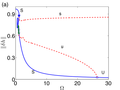
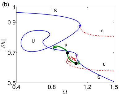
Figure 14: (Color online) (a) The complete bifurcation diagram for $\beta_{0}=1.4$ and $B=1$ giving the solution measure $\|\delta h\|$ in dependence on the rotation number $\Omega$. The steady-state branch is shown by the (blue) solid line. The various time-periodic branches are shown by the (red) dashed and (green) thick solid lines. Panel (b) shows a zoom of panel (a) into the small-$\Omega$ region ($0.4\leq\Omega\leq 1.5$) where most of the bifurcation structure is located. The filled black circles on the (green) thick solid line of time-periodic solutions indicate torus bifurcations, and the solutions on the part of the branch between these points are stable.

Comparing the cases of $\beta_{0}=2$ in Fig. 10 and of $\beta_{0}=1.4$ in Fig. 14, we notice that in both cases the time-periodic branch emerges from the rightmost HB (at $\Omega\approx 16.4$ and $26.3$ for $\beta_{0}=2$ and $1.4$, respectively) and terminates at another HB. However, this structure changes at smaller $\beta_{0}$. As shown in Fig. 15(a) for $\beta_{0}=1.348$, there appear two additional HCs at $\Omega\approx 0.94$ and $0.97$. The time-periodic branch emerging from the rightmost HB now terminates at the HC at $\Omega\approx 0.97$ and, correspondingly, the HB at $\Omega=1.05$ terminates at the HC at $\Omega\approx 0.94$. We note that all the remaining structures are the same between $\beta_{0}=1.4$ and $1.348$. There is one steady-state branch and two more time-periodic branches, where one emerges in a SNIPER bifurcation and the other one connects two HBs.

Going further down in $\beta_{0}$, at $\beta_{0}=1.343$ there appear two more HCs (at $\Omega\approx 0.915$ and $0.925$) that are connected by a new time-periodic branch, (brown) thick dashed line in Fig. 15(b). This new branch has again disappeared at $\beta=1.34$ (Fig. 15(c)). Then, at $\beta_{0}=1.3$ as shown in Fig. 15(d), the time-periodic branch emerging from the rightmost HB and the time-periodic branch emerging in a SNIPER bifurcation now merge into one single branch. As a consequence, the SNIPER bifurcation and one HC bifurcation disappear.

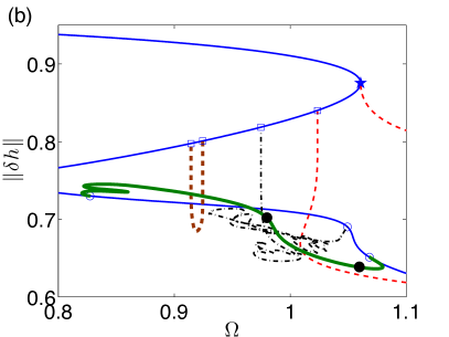
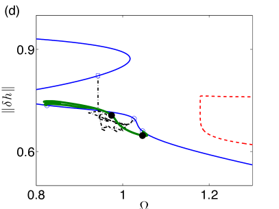
Figure 15: (Color online) The zoom-ins of the bifurcation diagrams in the small-$\Omega$ regions showing how the branches/bifurcations evolve with decreasing $\beta_{0}$. (a) $\beta_{0}=1.348$; (b) $\beta_{0}=1.343$; (c) $\beta_{0}=1.34$; (d) $\beta_{0}=1.3$. The steady-state branch is shown by the (blue) solid line. The various time-periodic branches are shown by the (red) dashed, (green) thick solid, (brown) thick dashed and (black) dot-dashed lines. The filled black circles on the (green) thick solid lines of time-periodic solutions indicate torus bifurcations. As the figure aims at illustrating the various reconnections, the branch stabilities are not indicated. They can in part be deduced from Figs. 14 and 18.

Figure 16: (Color online) Numerical two-parameter continuation in the plane spanned by the contact angle, $\beta_{0}$, and the rotation number, $\Omega$. Shown are (i) the loci of the saddle-node bifurcation that at $\beta_{0}=2$ ‘hosts’ the SNIPER bifurcation by the (black) solid line and (ii) the loci of time-periodic solutions very close to the global bifurcation by the (blue) dashed line. Here, the temporal period is fixed to equal $1000$. (Red) circles, (green) squares and (black) stars correspond to period-$1000$ time-periodic solutions at $\beta_{0}=1.34$, $1.343$ and $1.348$, respectively.

To analyze in more detail how the branches/bifurcations appear and disappear, we perform continuations on the SNIPER and HC bifurcations to see how they evolve as $\beta_{0}$ varies. First, we focus on the SN that for $\beta_{0}=2$ is located at $\Omega\approx 1.68$ and perform a two-parameter fold-continuation in $\Omega$ and $\beta_{0}$ for decreasing $\beta_{0}$. The results is the (black) solid line in Fig. 16. Each of its points represents the location of an SN at the corresponding $\beta_{0}$. Next, we take a time-periodic solution for $\beta_{0}=2$ that is very close to the SNIPER bifurcation and perform a similar two-parameter continuation at a fixed temporal period (here at $1000$). The result is the (blue) dashed line in Fig. 16 that itself folds back and forth several times. We note that the upper part of the line for $\beta_{0}\geq 1.338$ (about $\Omega\approx 1.06$) actually coincides with the SN branch indicating that we are indeed tracking the SNIPER bifurcation. At $\beta_{0}=1.338$ the dashed line folds back towards larger $\beta_{0}$ indicating that (i) for $\beta_{0}>1.338$ there exist a SNIPER and a homoclinic bifurcation, (ii) the two global bifurcations approach each other as $\beta_{0}$ decreases and (iii) annihilate each other at (or very near to) the SN about $\beta_{0}\approx 1.338$ thereby joining the two branches of time-periodic solutions. Or seeing the process as occurring for increasing $\beta_{0}$: The time-periodic solution branch that emerges from the HB at $\Omega\approx 38.7$ in Fig. 12(a) approaches the branch of unstable steady solutions when increasing $\beta_{0}$, hits it finally at $\beta_{0}\approx 1.338$ at (or very close to) the SN. The time-periodic branch splits and the two ends are glued to the steady branch as a SNIPER and an HC. Similar transitions have been analyzed in the context of line formation in Langmuir-Blodgett transfer described via an amended Cahn-Hilliard equation Köpf and Thiele (2014). Another glimpse at Fig. 16 indicates that this is not the full picture as the dashed line that represents the homoclinic bifurcation undergoes another three folds indicating several annihilation and creation events of pairs of homoclinic bifurcations and even the emergence of entire new branches. Following the dashed line further down to $\beta_{0}=1$, we find that it then corresponds to the single HC described above in Sec. IV.2.

With the obtained information, we are now able to describe how the branches change. For $\beta_{0}>1.3485$, there exists a SNIPER bifurcation and there are no HCs. With decreasing $\beta_{0}$, at $\beta_{0}\approx 1.3485$ one of the time-periodic branches touches the unstable part of the steady-state branch and splits into two branches. Each of the branches then terminates at the steady-state branch in an HC, see, e.g., the case of $\beta_{0}=1.348$ in Fig. 15(a). At $\beta_{0}\approx 1.3447$ one of the time-periodic branches touches again the unstable part of the steady-state branch that generates two more HCs that are connected by a new time-periodic branch, see, e.g., the case of $\beta_{0}=1.343$ in Fig. 15(b). This new branch disappears at $\beta_{0}\approx 1.3415$ when the two HCs annihilate each other. Finally, at $\beta_{0}\approx 1.338$ one of the HCs and the SNIPER annihilate each other and the two corresponding time-periodic branches join together, see, e.g., the case of $\beta_{0}=1.3$ in Fig. 15(d).

IV.4 Transition from a medium ($\beta_{0}=1$) to a small ($\beta_{0}\ll 1$) contact angle

As the rich structure of time-periodic states is also related to partial wettability, it has to simplify and ultimately disappear with decreasing the equilibrium contact angle $\beta_{0}$, similar to the changes observed for branches of steady states discussed in Sec. III.2. We have found that, as $\beta_{0}$ decreases, only the rightmost HB and the corresponding time-periodic branch survive. The location of the HB and the whole time-periodic branch move towards larger $\Omega$ as $\beta_{0}$ decreases. In fact, as explained in Appendix B.2, asymptotically one can show that there is always a HB located at large enough $\Omega$ for all non-zero $\beta_{0}$. Furthermore, we find that the location of the HB approaches infinity as $\beta_{0}$ approaches zero and the scaling is given by Eq. (52). As a result, we define the modified rotation number as

$$\Omega_{\beta_{0}}=\frac{\sqrt{5}h_{0}\beta_{0}\Omega}{9}.$$ (10)

Figure 17(a) shows the time-periodic branch for different values of $\beta_{0}$ with $\Omega_{\beta_{0}}$ as the horizontal axis. For each $\beta_{0}$, the HB is located where the respective branch starts. One can see that all the HBs are located close to $\Omega_{\beta_{0}}=1$, meaning that the scaling result obtained by the asymptotic analysis is in an excellent agreement with the numerical results. Besides, one can observe that the time-periodic branches are subcritical for $\beta_{0}=1$ and $0.5$, i.e., initially the branch turns towards smaller values of $\Omega_{\beta_{0}}$ before turning back towards larger values of $\Omega_{\beta_{0}}$ in an SN. However, as $\beta_{0}$ gets smaller, the HB where the time-periodic branch emerges becomes supercritical, see, e.g., the curves for $\beta_{0}=0.1$ and $0.01$. Then, the branch turns at first towards larger values of $\Omega_{\beta_{0}}$, before it undergoes two SNs. This implies that another range of multistability exists. For example, for $\beta_{0}=0.1$ and $\beta_{0}=0.01$ in Fig. 17(a) in the range $1\lesssim\Omega_{\beta_{0}}\lesssim 1.1$, there exist two stable and one unstable time-periodic states. Depending on the initial condition, the long-time solution may be either a large-amplitude droplet co-rotating with the cylinder or a small-amplitude surface wave co-rotating with the cylinder.

Figure 17: (Color online) (a) Time-periodic branches for different values of $\beta_{0}$. The horizontal axis is the modified rotation number $\Omega_{\beta_{0}}$ given by Eq. (10). (b) Locations of the numerically computed HBs (circles) and the corresponding asymptotic prediction (blue solid line) and locations of the numerically found SNs (red dot-dashed line) on the time-periodic branch in dependence on $\beta_{0}$.

In Fig. 17(b), we show the location of the numerically found HBs (circles) for various values of $\beta_{0}$ and the corresponding asymptotic predictions ((blue) solid line), Eq. (52). One can see that the two match very well indicating that the approximation provided by the asymptotic analysis is excellent and the location of the HB indeed scales as $\beta_{0}^{-1}$ as $\beta_{0}$ approaches zero. On the other hand, we show as a (red) dot-dashed line the location of the numerically found SN on the time-periodic branch. It is found that the scaling of the SN is also $\beta_{0}^{-1}$. As a result, we conclude that the whole time-periodic branch moves towards $\Omega=\infty$ as $\beta_{0}$ decreases to $0$, and the scaling is $\beta_{0}^{-1}$. That is, in the limiting case $\beta_{0}=0$, which corresponds to complete wetting, the time-periodic branch should disappear and there exists only the steady-state branch. See also the discussion in Appendix B.2.2.

IV.5 Other interesting phenomena

As shown in the previous sections, the transitions between the bifurcation diagrams involve several reconnections of branches and bifurcations. What we have explained so far is only part of the story. In fact, there exist some more complicated structures including, e.g., the appearance of the torus bifurcations mentioned in Sec. IV.2 and several codimension-two bifurcations involving two HBs that occur when varying $\beta_{0}$. We are not able to provide all the details of these, but we would like to point out a very interesting case occuring, e.g., for $\beta_{0}=1.5$.

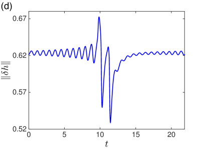
Figure 18: (Color online) (a) The zoom-in of the bifurcation diagram for $\beta_{0}=1.5$ and $B=1$. The graph style is the same as in Fig. 14. The filled black circles on the (green) thick solid line of time-periodic solutions indicate torus bifurcations, and the solutions on the part of the branch between these points are stable. (b) A schematic representation showing the connection of the time-periodic solution branch that shows tilted snaking and the time-periodic solution branch emerging from the HB. (c, d) Space-time contour plot and time evolution of the $L^{2}$-norm, $\|\delta h\|$, of the solution at the tilted snaking time-periodic solution branch at $\Omega=1.145$.

Figure 18(a) shows a zoom of the bifurcation diagram for $\beta_{0}=1.5$ and $B=1$. The steady-state branch is shown as the (blue) solid line and the time-periodic branches are shown as the (green) thick and (red) dashed lines to distinguish two different branches. In this figure, there exist three HBs and one HC. The time-periodic branch shown as the (red) dashed line is the one that emerges at the rightmost HB at large $\Omega$ outside the figure range. An interesting observation is that it actually terminates on another unstable time-periodic branch shown by the (green) thick line that itself ends nearby subcritically at an HB on the (blue) solid line representing the branch of steady states. A schematic representation of the connections is shown in panel (b) of the figure. We find that the (red) dashed time-periodic branch approaches the (green) thick branch along a tilted snaking path with its time-period approaching infinity. One of the solutions on the (red) dashed branch at $\Omega=1.145$ is presented in panels (c) and (d) showing the space-time contour plot and the time evolution of its $L^{2}$-norm, respectively. The time period for this solution is approximately $20.8468$. The solution profile corresponds to a pendent drop that continuously oscillates in time (small wiggles). This small-amplitude ‘background oscillation’ is interrupted by a temporally localized large-amplitude oscillation about $t=10$. The branch seems to approach the global bifurcation in a snaking manner with an ever decreasing amplitude of ‘wiggling’ in the bifurcation diagram. Each time the branch has completed one wiggle of the snake in Fig. 18(a), one more of the ‘background oscillations’ is added and the period increases by a fixed value (not shown). We expect that as the (red) dashed branch advances towards the bifurcation, the number of the wiggles approaches infinity and the period of the solution diverges. We also note that the solution profiles on the approached (green) thick branch correspond to single-frequency oscillations similar to the small-amplitude ‘background oscillations’.

V Conclusion

We have analyzed the behavior of a partially wetting liquid on a rotating cylinder using the long-wave model introduced in Ref. Thiele, 2011 as the governing equation. This model, in addition to accounting for the effects of gravity, viscosity, rotation and surface tension, includes the effect of wettability via the introduction of a Derjaguin (or disjoining) pressure term. Here, we have extended the preliminary results of Ref. Thiele, 2011 that was mainly concerned with the main depinning transition in two ways. We have shown that the complete bifurcation diagrams that describe continuous and discontinuous transitions between different steady and time-periodic thickness profiles and accompanying flow states are much richer than anticipated. This applies even to the case without rotation, not to speak of the case with driving where we have now discussed several branches of time-periodic solutions.

First, this has resulted in a deeper understanding of the specific case at large contact angle studied in Ref. Thiele, 2011. Second, and more importantly, we have analyzed how the bifurcation behavior (the depinning transition in particular) changes as the wettability is changed. In other words, we have investigated how the complex bifurcation structure found at large contact angles transforms into the much simpler behavior at zero contact angle. The calculations have been performed employing three approaches, namely, on one hand, different numerical continuation techniques that have allowed us to track stable and unstable steady and time-periodic states as well as, on the other hand, direct numerical simulations.

At equilibrium, the transition between complete and partial wetting corresponds to a phase transition called the wetting transition Bonn et al. (2009). A lateral driving force, like the one related to the rotation of the cylinder, brings the system permanently out of equilibrium and may cause a dynamic wetting transition. For instance, a thick film may be drawn out of a finite contact angle meniscus above a critical lateral driving Snoeijer et al. (2008); Galvagno et al. (2014) or an array of drops sliding down an incline may transform into a film Thiele et al. (2001). Placed within this wider context, the main purpose of the present study has been to investigate the interplay of depinning and wetting transitions for a specific well-defined system. In particular, we have analyzed in detail how the depinning behavior changes when the wettability of the liquid is increased [decreased], i.e., when the equilibrium contact angle is decreased [increased]. With this aim, we have determined bifurcation diagrams with the rotation number as the main control parameter for various values of the equilibrium contact angle.

As only a picture that contains all stable and unstable steady film and drop states and their relations allows one to understand the emerging complex dynamics, we have first completed the bifurcation diagrams of steady profiles for $\beta_{0}=2$ that beforeThiele (2011) were limited to a subset of the branches of steady-state solutions. In particular, we have discussed additional branches that represent unstable symmetric and asymmetric double-drop and double-hole (nucleation) solutions. Furthermore, we have shown that although triple-drop solutions do not exist on a resting cylinder (i.e., at equilibrium) at the chosen parameters, the non-equilibrium driving can bring them into existence when the cylinder is rotated.

In the second part, we have employed numerical continuation techniques to also determine all the branches of time-periodic solutions for various selected values of the contact angle. The completed bifurcation diagrams have allowed us to discuss how the global SNIPER bifurcation related to depinning of partially wetting drops disappears through a number of transitions when the contact angle is decreased towards small values. However, instead of the hoped-for simple scenario, where one branch of time-periodic solutions emerges from two separate ones when two global bifurcations collide on a branch of unstable steady solutions, we have encountered a rather intricate sequence of codimension-two bifurcations involving a dance of homoclinic bifurcations in the parameter plane, and a branch of tilted snaking of time-periodic solutions. This implies that the behavior is even more complicated than the behavior of the line deposition process described in Ref. Köpf and Thiele, 2014 that may also be seen as a depinning process, as discussed in Refs. Köpf et al., 2012; Frastia, Archer, and Thiele, 2012. It remains an interesting question how the described behavior is amended when further physical effects such as inertia and/or higher-order terms are incorporated, e.g., along the lines of Refs. Noakes, King, and Riley, 2006; Kelmanson, 2009, or if one goes beyond the long-wave (small physical contact angle) case and uses a full Stokes Hinch and Kelmanson (2003) or Navier-Stokes description incorporating wettability.

In addition to the numerical investigation, we have performed asymptotic analyses of steady-state solutions for zero rotation number and small contact angle, and of steady-state and time-periodic solutions for large rotation speeds, and found excellent agreement with the numerical results. We have also corroborated our findings by full time-dependent simulations of the underlying model.

The presented hydrodynamic system of a droplet on a rotating cylinder has been considered as a prototype for other depinning transitions in hydrodynamic systems, more general soft matter systems and beyond. These systems are characterized by an interplay of imposed spatial heterogeneity, a lateral driving force and a cohesive force resulting in coherent structures. As a weakening of the cohesive force will result in a first- or second-order phase transition (e.g., the wetting transition for the present system), the depinning transition will dramatically change its character in the proximity of the phase transition. However, our study has shown that the bifurcation behavior in the specific system studied is actually richer (more complicated) than expected. On one hand, this implies that the particular system of the rotating cylinder merits further studies and, on the other hand, it indicates that the quest for a simple though physically realistic model system is still open.

Appendix A Analysis of steady drops at $\Omega=0$

A.1 Drops at $B=0$ on an extended domain

Figure 19: (Color online) The bifurcation diagram for contact angle $\beta_{0}=2$ for the simplified system without gravity ($B=0$) and without rotation ($\Omega=0$) but for an extended domain size $L$ that is employed as the control parameter. The dotted vertical line indicates the value $L=2\pi$ that corresponds to our system in the chosen scaling. The various curves represent $n$-drop solutions upon the cylinder. The three crossings of branches and the vertical line represent one stable single-drop solution and two unstable double-drop solutions, which is consistent with the number of solution seen in Fig. 6 for $B=0$.

In this Appendix, we briefly consider the case $\Omega=0$, $B=0$ in an extended parameter space, to understand why Fig. 6 has to have at $\Omega=0$ and $B=0$ the two unstable double-drop solutions that give rise to the entire branch structure at $B>0$ even without driving. This will also allow us to understand why unstable triple-drop solutions may appear at finite $\Omega$. In particular, we continue $n$-drop solutions for $n=1,2,3,\dots$ in the domain size $L$. The result for $\beta_{0}=2$ is given in Fig. 19 where the vertical dotted line indicates $L=2\pi$ that is the normally fixed value for our system in the chosen scaling. The three intersections correspond to the three non-trivial steady thickness profiles at $B=0$ in Fig. 6, one single-drop and two double-drop profiles. This is a result of the subcritical character of the primary bifurcation in Fig. 19 that also explains why part of the solutions correspond to unstable nucleation (or hole) solutions (see discussions in Refs. Thiele and Knobloch, 2004 and Thiele et al., 2002).

There are no intersections of the vertical line with the unstable solution branches for $n\geq 3$ (three drops and above) and, therefore, there are no ‘equilibrium’ solutions at $\Omega=0$ with more than two drops. However, as triple-drop solutions exist at equilibrium at parameters not very far away from the considered system (at $L\approx 8$ in Fig. 19), the non-equilibrium driving can bring them into existence also at $L=2\pi$, i.e., the circumference of the cylinder in our scaling. Here, this occurs for $B=1$ between $\Omega\approx 0.68$ and $0.95$ (Figs. 3(b) and 5). This observation might be relevant for a number of other systems.

A.2 Changes in steady double-drop profiles with increasing Bond number

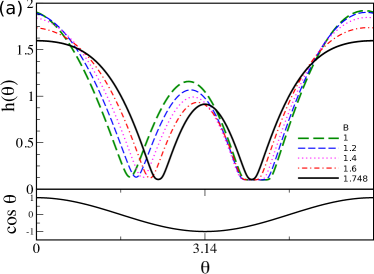
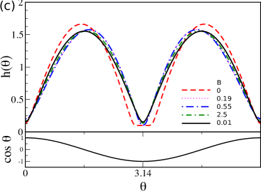
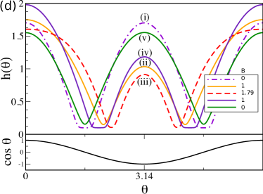
Figure 20: (Color online) Shown are selected double-drop profiles at various Bond numbers on the different branches in Fig. 6 for $\Omega=0$ and $\beta_{0}=2$. Panel (a) gives profiles along the asymmetric branch a$\mathrm{1}$ between $B=1$ and the pitchfork bifurcation at $B\approx 1.748$. The profiles on a$\mathrm{2}$ are obtained as mirror images about $\theta=\pi$. Panel (b) gives profiles along a$\mathrm{1}$ between $B=0.19$ and $B=1$. Panel (c) shows profiles along the symmetric branches d$\mathrm{l}$ and n$\mathrm{l}$. The order of the legend corresponds to the order of solutions if one were to follow the branch. Panel (d) gives profiles along the symmetric branches d$\mathrm{u}$ and n$\mathrm{u}$. Thereby, label (i) gives the solution with $\|\delta h\|\approx 0.57$ at $B=0$, then labels increase as one travels along the branches, until label (v) gives the solution with $\|\delta h\|\approx 0.46$ at $B=0$.

In this Appendix, we give some further details of the behavior of the double- drop solutions in Fig. 6.

We consider the left-shifted asymmetric drop profiles on the central a$\mathrm{1}$ branch and describe the changes in the drop profiles as $B$ varies. For any of the values of $B$ shown, the right-shifted asymmetric drop on the a$\mathrm{2}$ branch is obtained by considering the mirror image about $\theta=\pi$. For $B>1$ (Fig. 20(a)) the drop underneath the cylinder decreases in height and volume, while the larger drop on top of the cylinder increases its volume as liquid is transferred. Simultaneously, the short film between the drops decreases in length, because the volume of the larger drop increases but its height decreases. At $B\approx 1.748$, the gap between the drops disappears, the solution becomes symmetric and a$\mathrm{1}$ and a$\mathrm{2}$ terminate on n$\mathrm{u}$ in a symmetry-breaking pitchfork bifurcation slightly before n$\mathrm{u}$ and d$\mathrm{u}$ annihilate in the saddle-node bifurcation at $B\approx 1.749$. Moving on a$\mathrm{1}$ from $B=1$ in the opposite direction (Fig. 20(b)), we observe that the drop beneath the cylinder increases in height and volume, while the larger drop on top becomes smaller. The sizes of the gaps between the drops remain nearly the same, but the drops shift. At $B=0.19$ the solution itself has recovered the mirror symmetry at $\theta=\pi$ and the branches a$\mathrm{1}$ and a$\mathrm{2}$ end in a pitchfork bifurcation on d$\mathrm{l}$.

The steady profiles on the symmetric branches d$\mathrm{l}$ and n$\mathrm{l}$ (Fig. 6) show two drops of equal height arranged in a symmetric way about $\theta=\pi$ that are positioned on the sides of the cylinder, i.e., the holes are on top and underneath. The steady-state solution with the larger $L^{2}$-norm (on d$\mathrm{l}$), features at $B=0$ a flat film underneath the cylinder separating the drops, while the edges of the drops meet above the cylinder (Fig. 20(c)). Following this branch of steady-state solutions first along d$\mathrm{l}$ then along n$\mathrm{l}$ to the solution of smaller $L^{2}$-norm at $B=0$, the norm monotonically decreases since the separating flat film shrinks and the drops decrease in height. Selected profiles on the other symmetric branches d$\mathrm{u}$ and n$\mathrm{u}$ (Fig. 6) are given in Fig. 20(d). At $B=0$ on d$\mathrm{u}$ ($\|\delta h\|\approx 0.57$), there exist two identical drops on top and underneath the cylinder while the earlier discussed d$\mathrm{l}$ is the same solution shifted by $\pi/2$. They only start to differ once gravity is turned on, i.e., for $B\geq 0$. Moving along d$\mathrm{u}$ for increasing $B$, liquid is transferred to the drop on top and the films between the drops shrink until at $B\approx 1.749$ d$\mathrm{u}$ annihilates with n$\mathrm{u}$ in a saddle-node bifurcation. Returning on n$\mathrm{u}$, for decreasing $B$, the fluid transfers back to the drop beneath the cylinder and the drops reach again equal heights at $B=0$, where they correspond to standard nucleation solutions (cf. subcritical part of $n=3$ branch at $L=2\pi$ in Fig. 19).

Appendix B Asymptotic analysis for special cases

In Appendices B.1 and B.2, we analyze solutions in the limits of vanishing and infinite rotation numbers, respectively.

B.1 Steady-state solutions without rotation

The equation for the steady-state solutions when $\Omega=0$ is given by

$$\partial_{\theta}\left\{h^{3}\partial_{\theta}\left[\partial_{\theta}^{2}h+h-B\cos\theta+\Pi(h)\right]\right\}=0.$$ (11)

The equation can be integrated once, and the constant of integration can be removed because it represents the flux that is zero. We obtain

$$\partial_{\theta}\left[\partial_{\theta}^{2}h+h-B\cos\theta+\Pi(h)\right]=0.$$ (12)

Integrating the equation again, we have

$$\partial_{\theta}^{2}h+h-B\cos\theta+\Pi(h)=c,$$ (13)

where $c=1+\frac{1}{2\pi}\int^{2\pi}_{0}\Pi(h)\,d\theta$ is a constant.

For partially wetting liquids, $\beta_{0}\neq 0$, we have numerically found that there exists a finite number of distinct (in the sense that the solutions are not obtained from each other by a shift in $\theta$) non-trivial solutions (e.g., three non-trivial solutions for $\beta_{0}=2$ and $B=0$ as shown in Figs. 6 and 19), in addition to the trivial solution, $h_{0}\equiv 1$. Multiple non-trivial solutions exist up to a certain critical Bond number. Beyond the critical value (e.g., $B\approx 1.68$ for $\beta_{0}=2$) only the symmetric pendent drop solution exits.

On the other hand, for completely wetting liquids, the general solution of Eq. (13) can be written in the form

$$h_{c}=1+\frac{B}{2}\left(1+\theta\sin\theta\right)+A_{0}\sin\theta+A_{1}\cos\theta,$$ (14)

where $A_{0}$ and $A_{1}$ are constants. If $B=0$, we obtain an infinite number of $2\pi$-periodic solutions. However, for a non-zero $B$, $h_{c}$ is not a smooth $2\pi$-periodic function. That is, for a non-zero Bond number no classical solution exists Reisfeld and Bankoff (1992); Evans, Schwartz, and Roy (2004). We, therefore, consider a weak formulation. Our numerical results indicate that as $\beta_{0}\rightarrow 0$, a solution of Eq. (13) approaches a shape with a compact support. This can be see in Fig. 21(a), where steady pendent drop solutions are shown for various values of $\beta_{0}$. We note that such compactly-supported weak solutions were also found in heated-film systems as “dissipative compactons” Shklyaev, Straube, and Pikovsky (2010). Self-similar compactly-supported solutions were studied Witelski (1998); King (2001); Bernoff and Witelski (2002); Witelski, Bernoff, and Bertozzi (2004) and the stability was analyzed by Laugesen et al. Laugesen and Pugh (2002).

We see that there exists a thin precursor layer for partially wetting liquids and the thickness of the thin layer decreases to zero as $\beta_{0}$ approaches zero. The fact that the precursor can go continuously to zero can be realized by a scaling argument. If $\beta_{0}$ is fixed, then in the asymptotic limit $h_{0}\rightarrow 0$, using the asymptotic expansion in $h_{0}$, i.e., $h=h_{0}f_{0}+h_{0}^{2}f_{1}+\cdots$, we find that the leading-order equation requires $f_{0}=1$, i.e., there exists a precursor film of thickness $h_{0}$ (plus higher-order corrections). On the other hand, if we assume that $h_{0}$ is small but fixed and consider the asymptotic limit $\beta_{0}\rightarrow 0$, we find that an appropriate scaling for the precursor thickness $h_{p}$ is $h_{p}\propto\beta_{0}^{1/3}$. Then, we find that in Eq. (13) $c=O(1)$ when $\beta_{0}\rightarrow 0$ and the leading-order balance gives the precursor film of thickness $h_{p}=\left(\frac{5}{3(c+B\cos\theta)}\right)^{1/6}h_{0}^{5/6}\beta_{0}^{1/3}+o(\beta_{0}^{1/3})$.

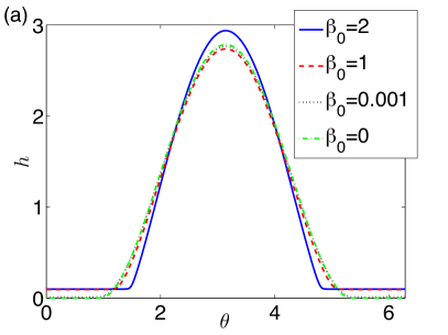
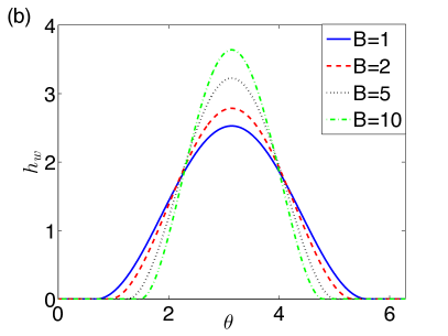
Figure 21: (Color online) (a) Steady-state solutions for partially wetting liquids at $B=2$ for various values of $\beta_{0}$. Note that the solution at $\beta_{0}=0$ is a weak solution given by Eq. (17). (b) Steady-state solutions for completely wetting liquids, $\beta_{0}=0$, for various values of $B$.

As a result, we use the following ansatz of a compactly-supported weak solution for the analytical expression of the asymptotic solution of completely wetting liquids Jensen (1997):

$$h_{w}(\theta)=\left\{\begin{array}[]{cc}c_{0}+\frac{B}{2}(\theta-\pi)\sin\theta+c_{1}\cos\theta,&\theta\in(\pi-\alpha,\pi+\alpha),\\ 0,&\theta\notin(\pi-\alpha,\pi+\alpha),\end{array}\right.$$ (17)

where $c_{0}$, $c_{1}$ and $\alpha$ are constants that should ensure that the solution $h_{w}$ satisfies the continuity and integral conditions:

$$h_{w}(\theta=\pi\pm\alpha)=\partial_{\theta}h_{w}(\theta=\pi\pm\alpha)=0,\quad\frac{1}{2\pi}\int^{2\pi}_{0}h_{w}\,d\theta=1.$$ (18)

Note also that for a purely macroscopic theory, i.e., without any disjoining pressure, weak solutions of partially wetting liquids can also be found by requiring $\partial_{\theta}h_{w}(\theta=\pi\pm\alpha)=\pm\beta_{e}$, where $\beta_{e}$ is the macroscopic equilibrium contact angle. For completely wetting liquids, $\beta_{e}=0$ and we obtain that the unknown constants $c_{0}$, $c_{1}$ and $\alpha$ should satisfy

$$\frac{\alpha^{2}}{\sin\alpha}+\alpha\cos\alpha-2\sin\alpha=\frac{2\pi}{B},$$ (19)

$$c_{0}=\frac{B}{2}\left(\cos\alpha+\frac{\alpha}{\sin\alpha}\right),$$ (20)

$$c_{1}=\frac{B}{2}\left(1+\frac{\alpha\cos\alpha}{\sin\alpha}\right).$$ (21)

Equations (19)-(21) can be solved numerically to obtain the constants of the asymptotic solution given by Eq. (17). The steady-state solutions for various Bond numbers are shown in Fig. 21(b). It is found that with decreasing $B$ the compact support of the solution becomes larger and the height of the central peak decreases. Besides, it can be shown that, in the limit $B\rightarrow 0$, we have $h_{w}=1-\cos\theta$.

B.2 Limit of large rotation number

B.2.1 Steady-state solutions

In the limit when $\Omega$ goes to infinity, it is appropriate to define the small parameter $\varepsilon=1/\Omega$ and rescale the time variable as $t=\varepsilon\tau$. Equation (1) can then be rewritten as

$$\partial_{\tau}h=-\partial_{\theta}h-\varepsilon\,\partial_{\theta}\left\{h^{3}\partial_{\theta}\left[\partial_{\theta}^{2}h+h-B\cos(\theta)+\Pi(h)\right]\right\}.$$ (22)

As suggested by numerical experiments, the $L^{2}$-norm of the steady-state solutions, as defined in Eq. (8), approaches zero and, therefore, the solutions approach the flat-film state. Hence, we expand the steady-state solution using the following ansatz

$$h_{s}(\theta)=1+\varepsilon h_{1}(\theta)+\varepsilon^{2}h_{2}(\theta)+\cdots.$$ (23)

Substituting the expansion into the equation for steady states, we can easily find the terms in the expansion. In particular, we find

$$h_{1}(\theta)=-B\sin(\theta),\quad h_{2}(\theta)=-\frac{3B^{2}}{2}\cos(2\theta)+\Pi^{\prime}(1)B\cos(\theta),$$ (24)

where we use the prime to denote the derivative of $\Pi$ with respect to $h$.

Next, we analyze the linear stability of the steady-state solution. Assuming that the solution is the steady state with a small perturbation, i.e., $h(\theta,\tau)=h_{s}(\theta)+\delta\eta(\theta,\tau)$, $\delta\ll 1$, we obtain the following linearized equation:

$$\eta_{\tau}=-\eta_{x}+\varepsilon\mathscr{L}[\eta],$$ (25)

where

$$\mathscr{L}[\eta]=-\partial_{\theta}\left\{h_{s}^{3}\partial_{\theta}[\partial_{\theta}^{2}\eta+(1+\Pi^{\prime}(h_{s}))\eta]+3h_{s}^{2}\partial_{\theta}[\partial_{\theta}^{2}h_{s}+h_{s}-B\cos(\theta)+\Pi(h_{s})]\eta\right\}.$$ (26)

Assuming that $\eta=e^{\lambda\tau}g(\theta)$, we have

$$\lambda g=-\partial_{\theta}g+\varepsilon\mathscr{L}[g].$$ (27)

By substituting the expansion (23) in (26), we can find

$$\mathscr{L}[\eta]=\mathscr{L}_{1}[\eta]+\varepsilon\mathscr{L}_{2}[\eta]+\cdots,$$ (28)

where

$$\mathscr{L}_{1}[\eta] = -\partial_{\theta}\{\partial_{\theta}^{3}\eta+(1+\Pi^{\prime}(1))\partial_{\theta}\eta+3\sin(\theta)\eta\},$$ (29)

$$\mathscr{L}_{2}[\eta] = -\partial_{\theta}\{[6Bh_{1}\sin(\theta)+(3+3\Pi^{\prime}(1)+\Pi^{\prime\prime}(1))\partial_{\theta}h_{1}+\partial_{\theta}^{3}h_{1}]\eta$$ (30)

$$+(3+3\Pi^{\prime}(1)+\Pi^{\prime\prime}(1))\partial_{\theta}h_{1}\partial_{\theta}\eta+3h_{1}\partial_{\theta}^{3}\eta\},$$

etc. We then expand $\lambda$ and $g$ in power series in $\varepsilon$, i.e., $\lambda=\lambda_{0}+\varepsilon\lambda_{1}+\cdots$ and $g=g_{0}+\varepsilon g_{1}+\cdots$, and substitute in (27). As a result, we obtain at $n^{\text{th}}$ order

$$\sum_{i=0}^{n}\lambda_{i}g_{n-i}=-\partial_{\theta}g_{n}+\sum_{i=1}^{n}\mathscr{L}_{i}[g_{n-i}].$$ (31)

At leading order, we have

$$\lambda_{0}g_{0}=-\partial_{\theta}g_{0},$$ (32)

and we obtain countably infinite number of solutions:

$$g_{0}^{k}(\theta)=e^{-\lambda_{0}^{k}\theta},\quad\lambda_{0}^{k}=ik,\quad k=0,\,\pm 1,\,\pm 2,\,\ldots.$$ (33)

We note that for each $k$, we can select an arbitrary amplitude for $g_{0}^{k}$, and we select it to be unity for convenience. At next order, we obtain the equation

$$\partial_{\theta}g_{1}^{k}+\lambda_{0}^{k}g_{1}^{k}=\mathscr{L}_{1}[g_{0}^{k}]-\lambda_{1}^{k}g_{0}^{k}.$$ (34)

Denoting the operator on the left-hand side by $\mathscr{M}^{k}$, i.e., $\mathscr{M}^{k}[f]\equiv\partial_{\theta}f+\lambda_{0}^{k}f$, it is easy to verify that $g_{0}^{k}$ is the basis for the null space of the adjoint operator $\mathscr{M}^{k*}$, defined by

$$\mathscr{M}^{k*}[f]\equiv-\partial_{\theta}f+\overline{\lambda_{0}^{k}}f,$$ (35)

where the overline denotes complex conjugation. Then, the Fredholm alternative solvability condition for the equation for $g_{1}^{k}$ requires that the inner product of the right-hand side of Eq. (34) and $g_{0}^{k}$ should vanish, which gives that

$$\lambda_{1}^{k}=\frac{\langle\mathscr{L}_{1}[g_{0}^{k}],g_{0}^{k}\rangle}{\langle g_{0}^{k},g_{0}^{k}\rangle}=(\Pi^{\prime}(1)+1)k^{2}-k^{4},\quad k=0,\,\pm 1,\,\pm 2,\,\ldots.$$ (36)

Note that if

$$\Pi^{\prime}(1)>0,$$ (37)

then at least for $k=\pm 1$, we obtain $\lambda_{1}^{k}>0$. Otherwise, all the $\lambda_{1}^{k}$’s are non-positive. Thus, if condition (37) is satisfied, at least two eigenvalues (the ones corresponding to $k=\pm 1$) have positive real parts (assuming that $\varepsilon$ is sufficiently small). In such a case, the steady solution is unstable. For the disjoining pressure given by Eq. (3),

$$\Pi^{\prime}(1)=-3H(1-2b).$$ (38)

Then, condition (37) is satisfied if $H>0$ and $b>1/2$ (which is an unphysical case), or $H<0$ and $b<1/2$. We note that our numerical findings agree with these theoretical conclusions. Namely, for a negative $H$ and sufficiently small $b$, we found in Sec. IV that on the branch of steady-state solutions there exists a subcritical Hopf bifurcation as $\Omega$ increases, and the steady solution becomes unstable. However, there exists a stable time-periodic solution. The analysis of such time-periodic solutions is given in the next section.

We would also like to point out that for completely wetting liquids, when $H=0$ , we find that $\lambda_{1}^{k}=0$ for $k=\pm 1$ and $\lambda_{1}^{k}<0$ for $|k|>1$. Hence, the stability cannot be determined at this order and higher-order terms are need to clarify the stability of the steady-state solutions for large values of $\Omega$.

Equation (31) for $n=2$ is

$$\partial_{\theta}g_{2}^{k}+\lambda_{0}^{k}g_{2}^{k}=\mathscr{L}_{1}[g_{1}^{k}]+\mathscr{L}_{2}[g_{0}^{k}]-\lambda_{1}^{k}g_{1}^{k}-\lambda_{2}^{k}g_{0}^{k}.$$ (39)

Then, the Fredholm alternative solvability condition implies that

$$\lambda_{2}^{k}=\frac{\langle\mathscr{L}_{1}[g_{1}^{k}]+\mathscr{L}_{2}[g_{0}^{k}]-\lambda_{1}^{k}g_{1}^{k},g_{0}^{k}\rangle}{\langle g_{0}^{k},g_{0}^{k}\rangle},\quad k=0,\,\pm 1,\,\pm 2,\,\ldots.$$ (40)

For $k=\pm 1$ (note that it is sufficient to consider $k=1$ since $\lambda_{n}^{-1}=\overline{\lambda_{n}^{1}}\,$), we find

$$\lambda_{2}^{1}=\frac{\langle\mathscr{L}_{1}[g_{1}^{1}]+\mathscr{L}_{2}[g_{0}^{1}],g_{0}^{1}\rangle}{\langle g_{0}^{1},g_{0}^{1}\rangle}.$$ (41)

By solving (34), we can find that

$$g_{1}^{1}(\theta)=-3iBe^{-2i\theta}+C_{1}e^{-i\theta},$$ (42)

where $C_{1}$ is an arbitrary constant. Next, substituting the expressions for $g_{0}^{1}$ and $g_{1}^{1}$ in (41), we find

$$\lambda_{2}^{1}=-\frac{15}{2}B^{2}i.$$ (43)

Since $\lambda_{2}^{\pm 1}$ are purely imaginary, we need to find the next order term.

Equation (31) for $n=3$ is

$$\partial_{\theta}g_{3}^{k}+\lambda_{0}^{k}g_{3}^{k}=\mathscr{L}_{1}[g_{2}^{k}]+\mathscr{L}_{2}[g_{1}^{k}]+\mathscr{L}_{3}[g_{0}^{k}]-\lambda_{1}^{k}g_{2}^{k}-\lambda_{2}^{k}g_{1}^{k}-\lambda_{3}^{k}g_{0}^{k}.$$ (44)

Then, the Fredholm alternative solvability condition implies that

$$\lambda_{3}^{k}=\frac{\langle\mathscr{L}_{1}[g_{2}^{k}]+\mathscr{L}_{2}[g_{2}^{k}]+\mathscr{L}_{3}[g_{0}^{k}]-\lambda_{1}^{k}g_{2}^{k}-\lambda_{2}^{k}g_{1}^{k},g_{0}^{k}\rangle}{\langle g_{0}^{k},g_{0}^{k}\rangle},\quad k=0,\,\pm 1,\,\pm 2,\,\ldots.$$ (45)

By solving (39) for $k=1$, we can find that $g_{2}^{1}(\theta)$. (Since the expression that we obtain is quite lengthy, we omit it here.) Next, substituting the expressions for $g_{0}^{1}$, $g_{1}^{1}$ and $g_{2}^{1}$ in (45) with $k=1$, we find

$$\lambda_{3}^{1}=B^{2}\left[-81+\frac{57}{2}\Pi^{\prime}(1)+6B^{2}\Pi^{\prime\prime}(1)+\frac{1}{4}\Pi^{\prime\prime\prime}(1)\right],$$ (46)

which for $H=0$ becomes

$$\lambda_{3}^{1}=-81B^{2}.$$ (47)

This means that for completely wetting liquids and sufficiently large $\Omega$, $\mathrm{Re}(\lambda^{k})<0$ for $k=\pm 1,\pm 2,\,\ldots,$ i.e., the steady solution $h_{s}(\theta)$ is stable. Therefore, the behavior at large rotation numbers for completely wetting and partially wetting liquids is completely different – for completely wetting liquids small-amplitude steady solutions are stable, whereas for even slightly non-wetting liquids such steady solutions are unstable and, instead, stable large-amplitude time-periodic solutions emerge (see the next section for the analysis of such time-periodic solutions).

For a general partially wetting liquid, we find

$$\mathrm{Re}(\lambda^{1})=\varepsilon\Pi^{\prime}(1)+\varepsilon^{3}B^{2}\left[-81+\frac{57}{2}\Pi^{\prime}(1)+6B^{2}\Pi^{\prime\prime}(1)+\frac{1}{4}\Pi^{\prime\prime\prime}(1)\right]+O(\varepsilon^{4}),$$ (48)

which allows to estimate the value of the angular velocity $\Omega$ at which the steady-state solution looses stability and a time-periodic solution emerges. Indeed, using (48), we find that the condition $\mathrm{Re}(\lambda^{1})=0$ implies that the Hopf bifurcation occurs at

$$\varepsilon\approx\frac{1}{B}\sqrt{\frac{\Pi^{\prime}(1)}{\left[81-\frac{57}{2}\Pi^{\prime}(1)-6B^{2}\Pi^{\prime\prime}(1)-\frac{1}{4}\Pi^{\prime\prime\prime}(1)\right]}},$$ (49)

(which is consistent with the assumption that $\varepsilon\ll 1$ when $\Pi^{\prime}(1)\ll 1$ and/or $B\gg 1$). Since $\varepsilon=1/\Omega$, condition (49) is equivalent to

$$\Omega\approx B\sqrt{\frac{\left[81-\frac{57}{2}\Pi^{\prime}(1)-6B^{2}\Pi^{\prime\prime}(1)-\frac{1}{4}\Pi^{\prime\prime\prime}(1)\right]}{\Pi^{\prime}(1)}}.$$ (50)

For the disjoining pressure given by (3), this condition becomes

$$\Omega\approx B\sqrt{\frac{54+19H-2Hb}{-2H(1-2b)}}.$$ (51)

Considering the small-contact-angle limit, $\beta_{0}\ll 1$, and using that $H=-\frac{5}{3}\beta_{0}^{2}h_{0}^{2}$, we obtain the following scaling for the Hopf bifurcation point:

$$\Omega\approx\frac{9B}{\sqrt{5}h_{0}}{\beta_{0}^{-1}}.$$ (52)

We note, however, that this condition corresponds to the case when the first two terms in the asymptotic expansion for $\lambda^{1}$ become of the same order, i.e., the asymptotic expansion strictly speaking breaks down. Therefore, for a more rigorous analysis, the case $\beta_{0}=O(\varepsilon)$ should be treated separately, although it would lead to the same condition (52).

B.2.2 Time-periodic solutions

To look for time-periodic solutions, we first impose a co-moving frame by defining $\xi=\theta-\tau$. Equation (22) is rewritten as

$$\partial_{\tau}h=-\varepsilon\,\partial_{\xi}\left\{h^{3}\partial_{\xi}\left[\partial_{\xi}^{2}h+h-B\cos(\xi+\tau)+\Pi(h)\right]\right\}.$$ (53)

Assuming that $h(\xi,\tau)=H_{0}(\xi,\tau)+\varepsilon H_{1}(\xi,\tau),+\cdots$, at leading order we have

$$\partial_{\tau}H_{0}=0.$$ (54)

That is, $H_{0}(\xi,\tau)=\phi_{0}(\xi)$ for some function $\phi_{0}$. Periodicity and the mean film thickness condition require that $\phi_{0}$ is $2\pi$-periodic and that $\int^{2\pi}_{0}\phi_{0}(x)dx=2\pi$, respectively. At next order, we obtain

$$\partial_{\tau}H_{1}=-\partial_{\xi}\left\{H_{0}^{3}\partial_{\xi}\left[\partial^{2}_{\xi}H_{0}+H_{0}-B\cos(\xi+\tau)+\Pi(H_{0})\right]\right\}.$$ (55)

Integration with respect to $\tau$ over $[0,2\pi]$ gives

$$\partial_{\xi}\left\{H_{0}^{3}\partial_{\xi}\left[\partial^{2}_{\xi}H_{0}+H_{0}+\Pi(H_{0})\right]\right\}=0.$$ (56)

By integrating this equation with respect to $\xi$, we find

$$H_{0}^{3}\partial_{\xi}\left[\partial^{2}_{\xi}H_{0}+H_{0}+\Pi(H_{0})\right]=c_{2},$$ (57)

where $c_{2}$ is a constant. One more integration, after dividing by $H_{0}^{3}$, implies that $c_{2}$ should be zero. Therefore, we obtain

$$\partial_{\xi}\left[\partial^{2}_{\xi}H_{0}+H_{0}+\Pi(H_{0})\right]=0,$$ (58)

which after one more integration implies

$$\partial_{\xi}^{2}H_{0}+H_{0}+\Pi(H_{0})=c,$$ (59)

where $c$ is a constant. By integrating the latter equation once again and using the fact that the mean thickness is $1$, we actually find that $c=1+\frac{1}{2\pi}\int^{2\pi}_{0}\Pi(H_{0})d\xi$. Note that Eq. (59) is exactly the same as Eq. (13) for $B=0$. That is, in the limit of a large rotation number, the solution at leading order is a steady solution of zero Bond number co-rotating with the cylinder.

As discussed in Sec. III.1, for partially wetting liquids there exist three non-trivial large-amplitude solutions at zero Bond number. These are the solutions that can co-rotates with the cylinder at large rotation number. For completely wetting liquids at zero Bond number, on the other hand, there exist infinitely many solutions given by Eq. (14) with $B=0$. However, we will show in the following that only the trivial solution $H_{0}\equiv 1$ exists at large rotation number. For this, we need to go to higher orders.

From Eqs. (55) and (59) we find that

$$H_{1}=B\partial_{\xi}\left[H^{3}_{0}\cos(\xi+\tau)\right]+\phi_{1}(\xi),$$ (60)

where $\phi_{1}$ is of zero mean. To determine $\phi_{1}$, we consider the equation at next order:

$$\partial_{\tau}H_{2}=-\partial_{\xi}\left\{H_{0}^{3}\partial_{\xi}\left[\partial^{2}_{\xi}H_{1}+H_{1}\right]+3BH^{2}_{0}\sin(\xi+\tau)H_{1}\right\}.$$ (61)

Integration with respect to $\tau$ over $[0,2\pi]$ gives

$$\partial_{\xi}\left\{H_{0}^{3}\partial_{\xi}\left[\partial^{2}_{\xi}\phi_{1}+\phi_{1}\right]\right\}=\partial_{\xi}\left\{\frac{3}{2}B^{2}H^{5}_{0}\right\}.$$ (62)

We denote the linear operator on the left-hand side by $\mathscr{K}$, and find that its adjoint operator is

$$\mathscr{K}^{*}[g]=\partial^{3}_{\xi}\left\{H_{0}^{3}\partial_{\xi}g\right\}+\partial_{\xi}\left\{H_{0}^{3}\partial_{\xi}g\right\}.$$ (63)

It can be easily shown that $\int\frac{\sin\xi}{H_{0}^{3}}\,d\xi$ and $\int\frac{\cos\xi}{H_{0}^{3}}\,d\xi$ are in the null space of $\mathscr{K}$. Then, by the Fredholm alternative solvability condition, the right-hand side of Eq. (62) should be orthogonal to these two functions. This leads to

$$\int^{2\pi}_{0}H^{2}_{0}\sin\xi\,d\xi=\int^{2\pi}_{0}H^{2}_{0}\cos\xi\,d\xi=0.$$ (64)

For a completely wetting liquid, the general form of $H_{0}$ is $H_{0}=1+A_{0}\sin(\xi)+A_{1}\cos(\xi)$. It can be easily seen that the latter integral conditions imply that $A_{0}=A_{1}=0$. Therefore, $H_{0}\equiv 1$. That is, for completely wetting liquids, there do not exist large-amplitude time-periodic solutions. Moreover, we find that for a completely wetting liquid

$$H_{1}=-B\sin(\xi+\tau)=-B\sin(\theta),$$ (65)

i.e., $H_{1}$ is in fact time-independent and is exactly the same as the order $\varepsilon$ term in the expansion of a small-amplitude steady solution, see Eq. (24). In fact, it can be shown that at all the orders the $H_{k}$’s are time-independent, and we recover the small-amplitude steady solution discussed in the previous section. We conclude that for the completely wetting case, time-periodic solutions do not exist for large values of $\Omega$, which is consistent with our numerical observations in Sec. IV.3.

References

- Moffatt (1977) H. K. Moffatt, “Behaviour of a viscous film on the outer surface of a rotating cylinder,” J. Mec. 16, 651 (1977).
- Ruschak (1985) K. J. Ruschak, “Coating flow,” Annu. Rev. Fluid Mech. 17, 65 (1985).
- Oron, Davis, and Bankoff (1997) A. Oron, S. H. Davis, and S. G. Bankoff, “Long-scale evolution of thin liquid films,” Rev. Mod. Phys. 69, 931–980 (1997).
- Pukhnachov (1977) V. V. Pukhnachov, “The liquid film motion on the rotating cylinder surface at the presence of gravity,” Prikl. Mekh. Teor. Fiz. 3, 77 (1977).
- Noakes, King, and Riley (2006) C. J. Noakes, J. R. King, and D. S. Riley, “On the development of rational approximations incorporating inertial effects in coating and rimming flows: a multiple-scales approach,” Q. J. Mech. Appl. Math. 59, 163–190 (2006).
- Kelmanson (2009) M. A. Kelmanson, “On inertial effects in the Moffatt-Pukhnachov coating-flow problem,” J. Fluid Mech. 633, 327–353 (2009).
- Hinch and Kelmanson (2003) E. J. Hinch and M. A. Kelmanson, “On the decay and drift of free-surface perturbations in viscous thin-film flow exterior to a rotating cylinder,” Proc. R. Soc. London Ser. A-Math. Phys. Eng. Sci. 459, 1193–1213 (2003).
- Karabut (2007) E. A. Karabut, “Two regimes of liquid film flow on a rotating cylinder,” J. Appl. Mech. Tech. Phys. 48, 55–64 (2007).
- Thiele (2011) U. Thiele, “On the depinning of a drop of partially wetting liquid on a rotating cylinder,” J. Fluid Mech. 671, 121 (2011).
- Starov and Velarde (2009) V. M. Starov and M. G. Velarde, “Surface forces and wetting phenomena,” J. Phys.-Condens. Matter 21, 464121 (2009).
- Thiele and Knobloch (2006a) U. Thiele and E. Knobloch, “Driven drops on heterogeneous substrates: Onset of sliding motion,” Phys. Rev. Lett. 97, 204501 (2006a).
- Herde et al. (2012) D. Herde, U. Thiele, S. Herminghaus, and M. Brinkmann, “Driven large contact angle droplets on chemically heterogeneous substrates,” Europhys. Lett. 100, 16002 (2012).
- Varagnolo et al. (2013) S. Varagnolo, D. Ferraro, P. Fantinel, M. Pierno, G. Mistura, G. Amati, L. Biferale, and M. Sbragaglia, “Stick-slip sliding of water drops on chemically heterogeneous surfaces,” Phys. Rev. Lett. 111, 066101 (2013).
- Sbragaglia et al. (2014) M. Sbragaglia, L. Biferale, G. Amati, S. Varagnolo, D. Ferraro, G. Mistura, and M. Pierno, “Sliding drops across alternating hydrophobic and hydrophilic stripes,” Phys. Rev. E 89, 012406 (2014).
- Thiele and Knobloch (2006b) U. Thiele and E. Knobloch, “On the depinning of a driven drop on a heterogeneous substrate,” New J. Phys. 8, 313 (2006b).
- Beltrame et al. (2011) P. Beltrame, E. Knobloch, P. Hänggi, and U. Thiele, “Rayleigh and depinning instabilities of forced liquid ridges on heterogeneous substrates,” Phys. Rev. E 83, 016305 (2011).
- Frastia, Archer, and Thiele (2012) L. Frastia, A. J. Archer, and U. Thiele, “Modelling the formation of structured deposits at receding contact lines of evaporating solutions and suspensions,” Soft Matter 8, 11363–11386 (2012).
- Köpf et al. (2012) M. H. Köpf, S. V. Gurevich, R. Friedrich, and U. Thiele, “Substrate-mediated pattern formation in monolayer transfer: a reduced model,” New J. Phys. 14, 023016 (2012).
- Doumenc and Guerrier (2013) F. Doumenc and B. Guerrier, “Self-patterning induced by a solutal Marangoni effect in a receding drying meniscus,” Europhys. Lett. 103, 14001 (2013).
- Thiele (2014) U. Thiele, “Patterned deposition at moving contact line,” Adv. Colloid Interface Sci. 206, 399–413 (2014).
- Köpf and Thiele (2014) M. H. Köpf and U. Thiele, “Emergence of the bifurcation structure of a Langmuir–Blodgett transfer model,” Nonlinearity 27, 2711 (2014).
- Ben Amar, Cummings, and Pomeau (2001) M. Ben Amar, L. Cummings, and Y. Pomeau, “Singular points of a moving contact line,” C R Acad. Sci. Ser. IIB 329, 277–282 (2001).
- Snoeijer et al. (2008) J. H. Snoeijer, J. Ziegler, B. Andreotti, M. Fermigier, and J. Eggers, “Thick films of viscous fluid coating a plate withdrawn from a liquid reservoir,” Phys. Rev. Lett. 100, 244502 (2008).
- Ziegler, Snoeijer, and Eggers (2009) J. Ziegler, J. Snoeijer, and J. Eggers, “Film transitions of receding contact lines,” Eur. Phys. J.-Spec. Top. 166, 177–180 (2009).
- Galvagno et al. (2014) M. Galvagno, D. Tseluiko, H. Lopez, and U. Thiele, “Continuous and discontinuous dynamic unbinding transitions in drawn film flow,” Phys. Rev. Lett. 112, 137803 (2014).
- Bonn et al. (2002) D. Bonn, D. Ross, E. Bertrand, K. Ragil, N. Shahidzadeh, D. Broseta, and J. Meunier, “Wetting transitions,” Physica A 306, 279–286 (2002).
- Bonn et al. (2009) D. Bonn, J. Eggers, J. Indekeu, J. Meunier, and E. Rolley, “Wetting and spreading,” Rev. Mod. Phys. 81, 739–805 (2009).
- Doedel, Keller, and Kernevez (1991) E. Doedel, H. B. Keller, and J. P. Kernevez, “Numerical analysis and control of bifurcation problems (I): Bifurcation in finite dimensions,” Int. J. Bifurcation Chaos 1, 493 (1991).
- Dijkstra et al. (2014) H. A. Dijkstra, F. H. Wubs, A. K. Cliffe, E. J. Doedel, I. F. Dragomirescu, B. Eckhart, A. Y. Gelfgat, A. Hazel, V. Lucarini, A. G. Salinger, E. P. Phipps, J. Sanchez-Umbria, H. Schuttelaars, L. S. Tuckerman, and U. Thiele, “Numerical Bifurcation Methods and their Application to Fluid Dynamics: Analysis beyond Simulation,” Commun. Comput. Phys. 15, 1 (2014).
- de Gennes (1985) P.-G. de Gennes, “Wetting: Statics and dynamics,” Rev. Mod. Phys. 57, 827–863 (1985).
- Israelachvili (2011) J. N. Israelachvili, Intermolecular and Surface Forces, 3rd ed. (Academic Press, London, 2011).
- Pismen (2001) L. M. Pismen, “Nonlocal diffuse interface theory of thin films and the moving contact line,” Phys. Rev. E 64, 021603 (2001).
- Pismen and Thiele (2006) L. M. Pismen and U. Thiele, “Asymptotic theory for a moving droplet driven by a wettability gradient,” Phys. Fluids 18, 042104 (2006).
- Kuznetsov (2010) Y. A. Kuznetsov, Elements of Applied Bifurcation Theory, 3rd ed. (Springer, New York, 2010).
- Doedel and Oldeman (2009) E. J. Doedel and B. E. Oldeman, AUTO07p: Continuation and bifurcation software for ordinary differential equations (Concordia University, Montreal, 2009).
- Thiele et al. (2001) U. Thiele, M. G. Velarde, K. Neuffer, M. Bestehorn, and Y. Pomeau, “Sliding drops in the diffuse interface model coupled to hydrodynamics,” Phys. Rev. E 64, 061601 (2001).
- Tseluiko, Galvagno, and Thiele (2014) D. Tseluiko, M. Galvagno, and U. Thiele, “Collapsed heteroclinic snaking near a heteroclinic chain in dragged meniscus problems,” Eur. Phys. J. E 37, 33 (2014).
- Tseluiko, Baxter, and Thiele (2013) D. Tseluiko, J. Baxter, and U. Thiele, “A homotopy continuation approach for analysing finite-time singularities in thin liquid films,” IMA J. Appl. Math. 78, 762–776 (2013).
- Thiele and Knobloch (2006c) U. Thiele and E. Knobloch, “On the depinning of a driven drop on a heterogeneous substrate,” New J. Phys. 8, 313 (2006c).
- Thiele, Kamps, and Gurevich (2014) U. Thiele, O. Kamps, and S. V. Gurevich, eds., Münsteranian Torturials on Nonlinear Science: Continuation (CeNoS, Münster, 2014) http://www.uni-muenster.de/CeNoS/Lehre/Tutorials.
- Bordyugov and Engel (2007) G. Bordyugov and H. Engel, “Continuation of spiral waves,” Physica D 228, 49–58 (2007).
- Pototsky, Thiele, and Archer (2014) A. Pototsky, U. Thiele, and A. Archer, “Coarsening modes of clusters of aggregating particles,” Phys. Rev. E 89, 032144 (2014).
- Pototsky et al. (2011) A. Pototsky, A. J. Archer, S. E. Savel’ev, U. Thiele, and F. Marchesoni, “Ratcheting of driven attracting colloidal particles: Temporal density oscillations and current multiplicity,” Phys. Rev. E 83, 061401 (2011).
- Reisfeld and Bankoff (1992) B. Reisfeld and S. G. Bankoff, “Non-isothermal flow of a liquid film on a horizontal cylinder,” J. Fluid Mech. 236, 167–196 (1992).
- Evans, Schwartz, and Roy (2004) P. L. Evans, L. W. Schwartz, and R. V. Roy, “Steady and unsteady solutions for coating flow on a rotating horizontal cylinder: Two-dimensional theoretical and numerical modeling,” Phys. Fluids 16, 2742 (2004).
- Strogatz (1994) S. H. Strogatz, Nonlinear Dynamics and Chaos (Westview Press, 1994).
- Hazel (2014) A. L. Hazel, “Personal communication,” (2014).
- Thiele and Knobloch (2004) U. Thiele and E. Knobloch, “Thin liquid films on a slightly inclined heated plate,” Phys. D 190, 213 (2004).
- Pailha et al. (2012) M. Pailha, A. L. Hazel, P. A. Glendinning, and A. Juel, “Oscillatory bubbles induced by geometrical constraint,” Phys. Fluids 24, 021702 (2012).
- Thiele et al. (2002) U. Thiele, K. Neuffer, Y. Pomeau, and M. G. Velarde, “On the importance of nucleation solutions for the rupture of thin liquid films,” Colloid Surf. A 206, 135–155 (2002).
- Shklyaev, Straube, and Pikovsky (2010) S. Shklyaev, A. V. Straube, and A. Pikovsky, “Superexponential droplet fractalization as a hierarchical formation of dissipative compactons,” Phys. Rev. E 82, 020601 (2010).
- Witelski (1998) T. P. Witelski, “Equilibrium interface solutions of a degenerate singular Cahn-Hilliard equation,” Appl. Math. Lett. 11, 127 (1998).
- King (2001) J. R. King, “Two generalisations of the thin film equation,” Math. Comput. Model. 34, 737–756 (2001).
- Bernoff and Witelski (2002) A. J. Bernoff and T. P. Witelski, “Linear stability of source-type similarity solutions of the thin film equation,” Appl. Math. Lett. 15, 599 (2002).
- Witelski, Bernoff, and Bertozzi (2004) T. P. Witelski, A. J. Bernoff, and A. L. Bertozzi, “Blowup and dissipation in a critical-case unstable thin film equation,” Euro. J. Appl. Math. 15, 223–256 (2004).
- Laugesen and Pugh (2002) R. S. Laugesen and M. Pugh, “Energy levels of steady states for thin-film-type equations,” J. Differ. Equ. 182, 377 (2002).
- Jensen (1997) O. E. Jensen, “The thin liquid lining of a weakly curved cylindrical tube,” J. Fluid Mech. 331, 373–403 (1997).