First-generation Science Cases for Ground-based Terahertz Telescopes

Abstract

Ground-based observations at terahertz (THz) frequencies are a newly explorable area of astronomy for the next ten years. We discuss science cases for a first-generation 10-m class THz telescope, focusing on the Greenland Telescope as an example of such a facility. We propose science cases and provide quantitative estimates for each case. The largest advantage of ground-based THz telescopes is their higher angular resolution ($\sim 4$ arcsec for a 10-m dish), as compared to space or airborne THz telescopes. Thus, high-resolution mapping is an important scientific argument. In particular, we can isolate zones of interest for Galactic and extragalactic star-forming regions. The THz windows are suitable for observations of high-excitation CO lines and [N ii] 205 $\mu$m lines, which are scientifically relevant tracers of star formation and stellar feedback. Those lines are the brightest lines in the THz windows, so that they are suitable for the initiation of ground-based THz observations. THz polarization of star-forming regions can also be explored since it traces the dust population contributing to the THz spectral peak. For survey-type observations, we focus on “sub-THz” extragalactic surveys, whose uniqueness is to detect galaxies at redshifts $z\sim 1$–2, where the dust emission per comoving volume is the largest in the history of the Universe. Finally we explore possibilities of flexible time scheduling, which enables us to monitor active galactic nuclei, and to target gamma-ray burst afterglows. For these objects, THz and submillimeter wavelength ranges have not yet been explored.

1 Introduction

The access to the terahertz (THz) frequency range or far-infrared (FIR) wavelength range from the ground is mostly limited by the absorption of water vapor in the Earth’s atmosphere. Therefore, the THz region is one of the remaining unexplored wavelength ranges from the ground. Space, balloon-borne, and airborne observations have so far been used to explore THz astronomy. There are only limited sites on Earth where the THz windows are accessible, and ground-based THz astronomy is, indeed, possible. Greenland (Section 2.1), high-altitude ($>$5,000 m) Chilean sites (Matsushita et al., 1999; Paine et al., 2000; Matsushita & Matsuo, 2003; Peterson et al., 2003), and Antarctica (Yang et al., 2010a; Tremblin et al., 2011) are examples of suitable places for ground-based THz astronomy.

Even in those locations suitable for THz observations, the time of excellent weather is still limited. Therefore, observations need to be planned well in order to maximize the scientific output within the limited amount of observing time. Moreover, “first-generation” observations are especially important because they determine the direction of subsequent THz science. There have already been some pioneering efforts of ground-based THz observations such as with the Receiver Lab Telescope (RLT; Marrone et al. 2004), the Atacama Pathfinder Experiment (APEX; Wiedner et al. 2006), and the Atacama Submillimeter Telescope Experiment (ASTE; Shiino et al. 2013). However, the attempts by these existing facilities have been difficult and sparse due to challenging weather conditions. A dedicated telescope at an excellent site – as proposed for the GLT – is, thus, paramount for successful THz observations. In practice, such first-generation observations are associated with the development of THz detectors. Searching for targets that are relatively easy to observe but scientifically pioneering, is of fundamental importance to maximize the scientific value of the instrumental development. The first aim of this paper is, thus, to search for scientifically important and suitable targets for first-generation THz science cases.

The largest advantage of ground-based THz telescopes compared with space telescopes (e.g., Herschel; Pilbratt et al. 2010), airborne telescopes (e.g., the Stratospheric Observatory for Infrared Astronomy (SOFIA); Young et al. 2012), and balloon-borne telescopes is that it is possible to operate large dishes with a high diffraction-limited resolving capability. To clarify this advantage, it is convenient to have a specific telescope in mind in discussing science cases. In this paper, we focus on the Greenland Telescope (GLT). The GLT project is planning to deploy an Atacama Large Millimeter/submillimeter (ALMA)-prototype 12-m antenna to the Summit Station in Greenland (3,200 m altitude) for the purpose of using it as part of submillimter (submm) very long baseline interferometry (VLBI) telescopes (Inoue et al., 2014a, see also Section 2). Data of atmospheric transmission at the Summit Station have been accumulated over the past four years through our continuous monitoring campaign (Martin-Cocher et al., 2014, see also Section 2.2). Our analysis indicates that site conditions are suitable for a first-generation ground-based THz facility. Therefore, we mainly target the GLT in this paper, noting that the THz science cases will likely be similar or even common for all the first-generation THz telescopes except for their sky coverages.

This paper also provides a first basis for ground-based THz observations for later generations of telescopes with larger dishes, such as the initially proposed Cerro Chajnantor Atacama Telescope (CCAT) or any successor project. With a diameter twice as large as the GLT, these telescopes will have even better sensitivity and resolution to further push the scientific results achieved by the GLT.

One of the major scientific advantages of the THz regime is that thermal dust continuum emission will be measured around its peak in the spectral energy distribution (SED). Moreover, the angular resolution (4^′′ at 1.5 THz for the diffraction-limited primary beam) enables us to spatially resolve the individual star-formation sites within nearby molecular clouds, typically located within a distance of $\sim$300 pc (Section 3.1.1). This high resolution is also an advantage for extragalactic observations where star-formation activities within nearby galaxies will be resolved. (Section 3.3). We emphasize that a resolution of $\sim 4^{\prime\prime}$ is comparable to what is achieved with submm interferometers such as the Submillimeter Array (SMA; Ho, Moran, & Lo 2004), although ALMA can have a substantially better spatial resolution. No THz facility, including non-ground-based observatories, has ever routinely had such a resolution for imaging. For dust continuum, combining submm interferometric data with new 1.5 THz data will significantly improve dust temperature estimates.

A wealth of interesting but unexplored emission lines are also in the THz windows (Section 3.1). Highly exited rotational molecular lines (e.g., CO, HCN) will probe “extremely hot” (300–500 K) molecular regions, which have been missed in observations at longer wavelengths. Line profiles will reveal gas motions in these regions. Additional lines accessible in the THz windows will be groups of atomic fine-structure lines tracing diffuse transitional regions in the interstellar medium (ISM) from ionized or atomic gas to molecular gas, and pure rotational lines (e.g., CH) tracing chemically basic light molecules.

In summary, the THz frequencies are suitable for tracing some key chemical species in gas and solid materials often associated with star-formation activities. Therefore, the grand aim of THz science is to trace the processes in the ISM that lead to star formation (see Section 3 for more detailed discussion).

Since the weather conditions necessary for THz observations are only realized for a small fraction of the winter time (typically $\sim 10$%; Section 2.1), it is worth considering “sub-THz” observations as well (Section 4). Some survey observations in the 850 GHz and 650 GHz windows can be unique for THz telescopes, because these relatively high-frequency submm bands still remain difficult to be fully explored at those sites where the current submm telescopes are located.

We will also discuss the possibility of flexible scheduling of observing time, because the GLT will be capable of doing this. One of the largest advantages of such flexible time allocations is that we will be able to execute time-consuming surveys. We will also allocate monitoring and target-of-opportunity (ToO) observations. In the field of very-high-energy (VHE) phenomena, THz continuum observations can help to constrain the mechanism and region of origin of the VHE in active galactic nuclei (AGNs) and gamma-ray bursts (GRBs) (Section 5). In particular, current multi-frequency monitoring campaigns from optical to X- and gamma-rays lack observations at THz or sub-THz frequencies for a complete SED to constrain the underlying physics of the origin of VHE. THz continuum observations will provide clean measurements of the source intensity, without being affected by scintillation and extinction.

In this paper, we aim at exploring the scientific importance of ground-based THz observations, providing some quantitative estimates. For clarification, we focus on the GLT as one of the first-generation ground-based facilities, but the scientific discussions are general enough to be applied to any 10-m class THz telescope. This paper is organized as follows: we start by describing the features of the GLT as an example of future first-generation THz telescopes in Section 2. We discuss the key THz science cases in Section 3, and some sub-THz cases in Section 4. We also describe some science cases that are making maximal use of a flexible time allocation in Section 5. Based on the science cases discussed in this paper, we also summarize possible developments of future instruments in Section 6. Finally, we give a summary in Section 7. We use $(h,\,\Omega_{\mathrm{m}},\,\Omega_{\Lambda})=(0.71,\,0.27,\,0.73)$ for the cosmological parameters.

2 Project Overview and General Requirements

As emphasized above, the scope of this paper is not limited to a specific future project, but rather evaluating quantitatively some key science cases suitable for the first-generation ground-based THz telescopes. Here, we introduce the GLT as a typical telescope for this purpose, only to make clear what kind of capabilities would be expected in the near future for THz observations. We refer the interested reader to Inoue et al. (2014a) and Grimes et al. (2014) for the details of specifications and possible instruments for the GLT.

We also emphasize that, by considering the “realistic” case of the GLT, we will be able to extract the important aspects and requirements in performing ground-based observations. Indeed, as we demonstrate below, the following advantages of the GLT are of fundamental importance in realizing ground-based THz observations: (i) Atmospheric transmission (in the winter time, the atmospheric condition is statistically better than the Mauna Kea site (Martin-Cocher et al., 2014), and comparable to the ALMA site); (ii) stability of the atmospheric condition (in the winter time, there is no daylight and only minor daily temperature variations, so that the weather condition suitable for THz observations can last $>$ a day); (iii) flexible scheduling (except for the time occupied by the VLBI observations, the GLT can be used as a dedicated telescope for THz observations). In what follows, we will show that the GLT really has these advantages that are fundamentally important to the success of ground-based THz observations.

2.1 Brief introduction to the Greenland Telescope (GLT)

The GLT is an ALMA – North-American 12-m Vertex prototype antenna (Mangum et al., 2006) that is being retrofitted to arctic conditions, with the goal of deploying it to the Greenland Summit Station at an altitude of 3,200 m (located at latitude 7257N and longitude 3846W). Primary operating conditions for the GLT – defined as extending over 90% of the weather conditions – cover an ambient temperature down to $-50^{\circ}$C, wind speeds of up to 11 m s^-1 and a vertical temperature gradient (due to an inversion layer over the Greenlandic plateau) of $+7$ K over the antenna height from bottom to top. Furthermore, an ambient temperature change rate of up to 2 K hr^-1 is taken into account. Absolute (non-repeatable) pointing errors of 2with a final goal of 14 are targeted for primary conditions, together with offset pointing and tracking errors of 06 and a final 04. An antenna surface accuracy of 10 $\mu$m is targeted. For THz observations around 1.5 THz this yields an antenna surface efficiency of about 65%. This efficiency will drop to 40% and 20% for 15 $\mu$m and 20 $\mu$m surface accuracies. Secondary operating conditions – additionally covering the 90–95% range of weather occurrence – extend the ambient temperature further down to $-55^{\circ}$C and the wind speeds up to 13 m s^-1. A degraded antenna performance is accepted under these conditions.

The exceptionally dry atmospheric conditions at this site are suitable for submm and even for FIR (THz) observations (Section 2.2). The principal purpose of the GLT is to provide a submm-VLBI station that can be correlated with other telescopes such as the SMA, the James Clerk Maxwell Telescope (JCMT), and ALMA in order to achieve extremely long intercontinental baselines (Inoue et al., 2014a). This will greatly enhance the angular resolution at submm wavelengths. The key scientific goal of this interferometry is to measure the shadow caused by the strong gravitational field around the central supermassive black hole in M87. This project will provide a unique opportunity to study the strong general relativistic effects immediately surrounding the black hole’s event horizon. Related scientific topics include measuring the black hole spin in M87, constraining the nature of its accretion flow and determining the launching mechanism of its relativistic jet. Additional science cases are the very high energy emission in AGNs and the exploration of dark energy through high-precision measurements of locations and velocities of maser spots in galaxies.

The GLT will likely be used for VLBI observations only during a short period within each year (roughly 1–2 months), because many telescopes must be made available simultaneously. Therefore, we expect that a significant fraction of observing time can be used for single-dish observations. Below, we describe the capability of the GLT as a single-dish telescope.

2.2 Atmospheric condition

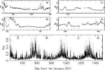
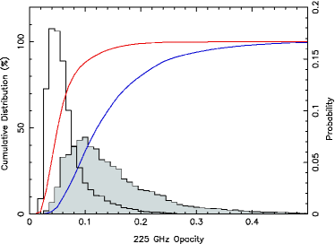
In 2011, we deployed a radiometer to Greenland to monitor the sky and weather conditions at the Summit Station (Martin-Cocher et al., 2014). The average temperature is low at around $-$30 to $-40^{\circ}$C, down to $-70^{\circ}$C in winter. Because of such low ambient temperatures, the water content in the air is exceedingly low. Every 10 minutes, a tipping measurement is performed to take opacity data. The measured 225 GHz atmospheric opacity as a function of time is shown in Figure 1.The corresponding histogram together with its cumulative distribution function (CDF) is depicted in Figure 2. We confirmed that the opacities lower quartile in these months can get as low as 0.047, with occasional opacities as low as 0.030 in the winter regime (November to April; see also the zoomed plots in Figure 1). Based on the monitoring opacity ($\tau$) data at 225 GHz, we estimated the precipitable water vapor (PWV), and then converted that into an atmospheric opacity at 1.5 THz using the “am” program and climatological data from Summit Camp for temperature, relative humidity and ozone profiles (Paine, 2012). For convenience, we give the conversion formula between $\tau$ and PWV in Figure 1. The observational rate with THz opacity ($\tau_{\mathrm{THz}}$) condition less than 2.0 and 3.0 were 1.8% and 11.4% in the winter regime (November to April). These fractions are similar to those expected for the ALMA site (2.0% for $\tau_{\mathrm{THz}}<2.0$ and 16.8% for $\tau_{\mathrm{THz}}<3.0$) in the winter season (Matsushita, 2011). It is noteworthy that THz opacity conditions giving $\tau_{\mathrm{THz}}<3.0$ can last from a few hours to half a day in many cases. In some cases, they last up to 3–7 days (see Figure 1a, b), which is only possible in the polar regions where there is no daylight in the winter time. If we focus on the months when such long durations of THz weather are achieved, the statistics of atmorpheric opacity at the Greenland Summit site are as good as at the Antarctic site. We also estimated the opacity condition less than 0.6 and 1.0 at sub-THz bands. Those were 8.2% and 32.9% at 675 GHz and 3.9% and 24.2% at 875 GHz, respectively.

Figure 1: Atmospheric opacity at 225 GHz from August 17th 2011 to February 7th 2015. Selected low opacity epochs of several days are indicated with the labels (a), (b), (c), (d) in the bottom plot. The zoomed-in plots are shown in the top four panels. The relation between the 225 GHz opacity $\tau$ and the PWV (in units of mm) was calculated with am (Paine, 2012), and expressed as $\tau=0.049\mathrm{PWV}+0.018$ (valid in October–May for $\tau<0.075$) or $\tau=0.047\mathrm{PWV}+0.015$ (valid in June–September for $\tau<0.2$).

Figure 2: Histograms of the 225 GHz opacity and cumulative distribution functions for the data shown in Fig. 1. The blue line and shaded histogram show the statistics in the summer months (May–October) while the red line and white histogram present the statistics in the winter months (November–April).

Tremblin et al. (2012) have presented the atmospheric conditions at various sites suitable for submm astronomy using satellite data, including Greenland. However, their data do not have a time resolution of less than $\sim$ a day, while time variations within a day are important for THz observations. Moreover, at the polar sites, the statistics focusing on the winter season is meaningful because the night continues over the whole winter period. We, therefore, think that our new opacity statistics is more reliable for the THz observing conditions.

Although Dome A in Antarctica would be better than the Greenland Summit Station, the GLT can play a unique role because it is still the best site in the northern hemisphere. In other words, the GLT and telescopes in Antarctica are complementary in their sky coverages. We emphasize that the science cases discussed in this paper are applicable to any THz telescope with a different fraction of time suitable for THz observations, as long as we adopt the same criterion for the THz weather ($\tau_{\mathrm{THz}}<2.0$ or 3.0).

2.3 Typical performance of the GLT

The expected observational performance of the GLT at the frequencies of atmospheric windows is summarized in Table 2.3, which is revised from Grimes et al. (2014), for the frequency range of interest in this paper (350–1,500 GHz). For this calculation, we assume the surface accuracy to be 15 $\mu$m. Indeed, the telescope was demonstrated to have a surface accuracy of 16 $\mu$m when it was at the evaluation phase as the ALMA prototype antenna (Mangum et al., 2006). Using the best 10% and median opacity conditions for the frequencies lower than 1 THz and the best 1.5% and the best 10% opacity conditions for the frequency higher than 1 THz at the winter season and the expected receiver performance (i.e., receiver temperature $T_{\mathrm{Rec}}$), we estimated the system temperature ($T_{\mathrm{sys}}$) for each frequency band, and corresponding continuum noise equivalent flux density for 1 second integration (NEFD) and spectral NEFD for 1 km s^-1 resolution.

Expected performance of the GLT. Frequency Resolution Transmission $T_{\mathrm{Rec}}$ $T_{\mathrm{sys}}$ Continuum NEFD Spectral NEFD (GHz) (arcsec) (%) (K) (K) (mJy s^1/2) [Jy s^1/2 (km s^-1)^1/2] 230 27 0.96 (0.91) 40 89 (110) 33 (41) 3.39 (4.18) 345 18 0.89 (0.82) 75 177 (192) 68 (73) 5.61 (6.06) 675 9.2 0.53 (0.28) 110 663 (1,510) 285 (648) 17.3 (39.4) 875 7.1 0.48 (0.24) 160 1,060 (2,450) 511 (1,190) 27.1 (63.0) 1020 6.1 0.16 (0.06) 525 9,110 (26,500) 5,120 (14,900) 245 (712) 1350 4.6 0.16 (0.06) 650 13,500 (36,100) 9,600 (25,600) 413 (1,100) 1500 4.1 0.15 (0.06) 750 20,300 (55,100) 17,900 (48,700) 718 (1,950) Note: This table is an updated version of Grimes et al. (2014); in this paper, we used the up-to-date opacity statistics mentioned in the previous subsection. Opacity, $T_{\mathrm{sys}}$, and NEFDs are given for two cases: the best 10% and median (in parenthesis) weather for the frequency lower than 1 THz, and the best 1.5% and the best 10% (in parenthesis) for the frequency higher than 1 THz. Both cases are based on the opacity statistics of the winter season (from November to April).

In practice, we typically consider to observe the sky area with a zenith angle $<60^{\circ}$. With the latitude of the site, $72^{\circ}$, therefore, we limit the declination to $\delta>12^{\circ}$.

2.4 Advantages of ground-based telescopes for THz astronomy

The advantage of ground-based observations is that we can use a large telescope. As shown in Section 2.3, the angular resolution achieved is about 4at 1.5 THz for a 10-m class ground-based telescope, while the diffraction limit of a 3.5-m-class space telescope, such as Herschel, is $\sim 12$around 1.5 THz. Thus, the obvious new parameter space to be explored by ground-based THz facilities is the angular resolution with an improvement of about an order of magnitude in beam area. In particular, no THz facility has ever routinely had such a resolution for imaging. Additional advantages are: (i) we can directly control and maintain the telescope; and (ii) we can run long-term projects which is difficult for non-ground-based facilities with limited lifetimes or limited observational durations.

As far as sensitivity is concerned, ground-based facilities cannot win over airborne or space telescopes even at the Summit Station in Greenland because of the atmospheric opacity. For example, a $\sim$30 times smaller continuum NEFD is achieved by the currently available airborne facility, SOFIA. Therefore, the first-generation ground-based THz telescopes need to focus on relatively bright objects where high-angular-resolution observations have the potential to do pioneering work.

2.5 Operations at sub-THz

Since the weather conditions suitable for THz observations are not guaranteed for all the winter time (typically $\sim 10$%; Section 2.2), operations at somewhat lower frequencies should also be considered. In order to be different from existing submm telescopes, we are taking advantage of the good atmospheric conditions to target relatively high frequencies, referred to as sub-THz in this paper. In particular, atmospheric windows around 850 GHz (350 $\mu$m) and 650 GHz (450 $\mu$m) are viable targets. Operations at submm/millimeter (mm)-wavelength sites like Mauna Kea have been rare in these frequency bands. The Greenland site will provide a significant fraction of time (Section 2.2) for these windows. Therefore, the second purpose of this paper is to identify compelling science cases in the shortest submm or sub-THz ranges.

A special advantage of the GLT is that it allows for flexible time scheduling. Time-consuming survey-type observations at sub-THz will be unique, because such observations are extremely difficult for practically all other telescopes in the northern hemisphere. This flexibility increases the chance to carry out monitoring and target-of-opportunity (ToO) observations. The scientific importance of this possibility is also explored in this paper.

3 THz Observations

3.1 Important lines at THz

In the THz regime there are a number of interesting but unexplored spectral lines, which should be useful for studies of the ISM and star formation. In line observations, sky background subtraction is much easier than in continuum observations, and thus observations of intense THz lines should be the starting point of our THz astronomical experiment. Table 3.1 summarizes representative THz lines whose rest-frame wavelengths are accessible in the THz atmospheric windows. These lines can be classified into three categories; (i) very high-$J$ ($J$ is the rotational excitation state) molecular lines (CO, HCO⁺, and HCN); (ii) atomic fine-structure lines ([N ii]); and (iii) pure rotational lines of light molecules (H₂D⁺, HD₂⁺, and CH).

Representative Tera-Hertz Lines. Species Frequency (THz) Transition Excitation energy (K) CO 1.037–1.497 (9–8)–(13–12) 248.87486–503.134028 HCO⁺ 1.070–1.337 (12–11)–(15–14) 333.77154–513.41458 HCN 1.0630–1.593 (12–11)–(18–17) 331.68253–726.88341 H₂D⁺ 1.370 1_0,1–0_0,0 65.75626 N ii 1.461 ³P₁–³P₀ — CH 1.471 N=2, J=3/2-3/2, F=2⁺–2^- 96.31131 HD${}_{2}^{+}$ 1.477 1_1,1–0_0,0 70.86548

3.1.1 Tracers of star-forming places

Kawamura et al. (2002) observed several positions in the Orion Molecular Cloud (OMC-1) by the ground-based 10-m Heinrich Hertz Telescope on Mount Graham, Arizona. They targeted the CO $J=9$–8 rotational line at 1.037 THz. They detected some regions with such a high excitation along the ridge of OMC-1. It has been clarified that there are some warm regions with kinetic temperatures $\gtrsim$130 K and hydrogen number density $\gtrsim 10^{6}$ cm^-3 in the molecular cloud. They also emphasized the importance of high angular resolutions achieved by ground-based telescopes in specifying the locations of the emission.

With the GLT, we aim at observing higher-excitation CO lines at a higher frequency, 1.5 THz, where CO $J=13$–12 (1.4969 THz) line is present. With the very high-$J$ molecular lines, “extremely hot” ($\gtrsim$300 K) molecular regions in the vicinity of the forming protostars can be traced. Moreover, CO is the most strongly emitting species in such a region, enabling us to trace lower-mass or more distant objects than other species. Profile shapes of those lines are probes of gas motions in such regions. Wiedner et al. (2006) built a 1.5 THz heterodyne receiver, CO N⁺ Deuterium Observations Reciever (CONDOR), installed it in the APEX, and performed ground-based THz line observations. With a total on-source time of 5.8 min, they detected CO ($J=13$–12) line toward Orion FIR 4, a cluster-forming region in the Orion Giant Molecular Cloud. The main beam brightness temperature and the line width of the THz CO line are $\sim 210$ K and $\sim 5.4$ km s^-1, respectively. As compared to the CO $J=9$–8 and 7–6 lines, there is no line wing component with $\gtrsim 10$ km s^-1 in the THz CO line. Multi-transitional analysis of the “quiescent” component of the CO lines show that the gas temperature and density traced by the THz line are $380\pm 70$ K and $(1.6\pm 0.7)\times 10^{5}$ cm^-3, respectively. These results show that the THz CO line traces the very hot molecular gas in the vicinity of the protostars, without any contamination from the extended outflow component. The bulk of the outflows are apparently at lower temperatures. With the GLT, we aim at a systematic survey of similar objects hosting highly excited CO lines.

Observations of submm and THz HCN lines toward Sgr B2(M) by Herschel/the Heterodyne Instrument for the Far-Infrared (HIFI) show that the submm HCN $J=6$–5 and 7–6 lines exhibit “blue-skewed” profiles suggestive of infall, while the HCN $J=8$–7 and the THz HCN $J=12$–11 (1.06 THz) lines exhibit “red-skewed” profiles suggestive of expansion (Rolffs et al., 2010). The submm HCN lines with the blue-skewed profiles originate from gas with temperature $\sim 100$ K while the THz line is emitted from gas with higher excitation $\sim 330$ K. These results suggest that the lower-$J$ HCN lines trace the outer infalling motion toward the massive stars, whereas the THz line traces the inner expansion driven by the radiation pressure and the stellar wind from the central massive stars. All of the above results imply that high-$J$ THz molecular lines can be unique tracers to probe the very inner parts of protostars and to study the gas motions there.

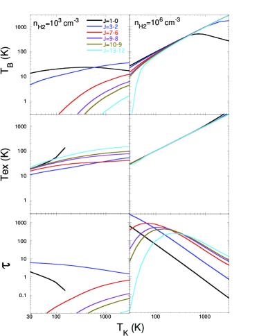
To quantify the physical conditions traced by THz high-$J$ molecular lines, we performed statistical equilibrium calculations of the CO lines based on the large velocity gradient (LVG) model (Goldreich & Kwan, 1974; Scoville & Solomon, 1974). For the calculations, the rotational energy levels, line frequencies, and the Einstein $A$ coefficients of CO are adopted from Leiden Atomic and Molecular Database (LAMDA; Schöier et al. 2005), and the collisional transition rates with ortho-H₂ from Yang et al. (2010b). The rotational energy levels up to $J=41$ (4,513 K) are included in the calculations. The formulae of the line profile function and photon escape probability of a static, spherically symmetric and homogeneous cloud are adopted (Osterbrock & Ferland, 2006). Our calculations are analogous to those of RADEX (van der Tak et al., 2007), and we confirmed that our codes provide the same results as those by RADEX.

Figure 3 shows the calculated line brightness temperatures ($T_{\mathrm{B}}$), excitation temperatures ($T_{\mathrm{ex}}$), and the optical depths ($\tau$) of the various CO lines as a function of the gas kinetic temperature ($T_{K}$) at an H₂ ($n_{\rm H_{2}}$) number density of 10³ cm^-3 and 10⁶ cm^-3. In the case of the diffuse molecular gas ($n_{\rm H_{2}}$ = 10³ cm^-3), the brightness temperatures of the THz CO lines ($J=9$–8, 10–9, and 13–12) are too low to be detected even at the very high gas temperatures, while those of lower-$J$ CO lines ($J=1$–0; 3–2) are high. This is because at the low gas density the higher $J$ levels are not populated and the THz CO lines are too optically thin, as shown in the lower-left panel. In contrast, at $n_{\rm H_{2}}$ = 10⁶ cm^-3, typical of dense cores (dense-gas condensations in molecular clouds), all CO transitions are thermalized and the excitation temperatures follow the gas kinetic temperature (middle-right panel). Consequently the optical depths, so the brightness temperatures, become high even for the THz lines. These results show that the THz CO lines are an excellent tracer of dense ($\gtrsim$10⁶ cm^-3) and hot ($\gtrsim$100 K) molecular gas.

Figure 3: Results of the statistical equilibrium calculations of the CO lines. The brightness temperatures (upper panels), excitation temperatures (middle panels), and the optical depths of the CO lines (lower panels) are plotted as a function of the gas kinetic temperature. In the left and right panels the number density of H₂ is set to be 10³ cm^-3 and 10⁶ cm^-3, respectively. The cloud size and velocity width are assumed to be 0.1 pc and 1.0 km s^-1, respectively, and the CO abundance relative to hydrogen is fixed as 9.5 $\times$ 10^-5 (Crapsi et al., 2004).

According to radiation-hydrodynamic models of protostar formation, such dense and high-temperature molecular regions should be present at the latest stage of protostellar collapse within $\sim 500$ AU from the forming central star (Masunaga & Inutsuka, 2000). For typical distances of protostellar sources ($d\sim 300$ pc), the diameter ($\sim$1,000 AU) corresponds to 3.3 arcsec, which roughly matches the angular resolution of the GLT at 1.5 THz ($\sim$ 4 arcsec; Section 2.3). With the GLT, thus, very hot molecular gas in the vicinity of the forming protostars can be observed. The line profile shape can then be used to trace the gas motions in such regions.

Luminous Protostellar Sources for the THz Line Experiment Name $L_{\mathrm{bol}}$ $D$ $\alpha$(J2000) $\delta$(J2000) Ref. ($L_{\odot}$) (pc) (h m s) (  ) L1448-mm 4.4 250 03 25 38 87 30 44 05.4 1,2 NGC1333 IRAS 2A 19.0 250 03 28 55.58 31 14 37.1 1,2 SVS 13 32.5 250 03 29 03.73 31 16 03.80 2,3 NGC1333 IRAS 4A 4.2 250 03 29 10.50 31 13 31.0 1,2 L1551 IRS 5 22 140 04 31 34.14 18 08 05.1 4,5 L1551 NE 4.2 140 04 31 44.47 18 08 32.2 5,6 L1157 5.8 325 20 39 06.28 68 02 15.8 1,7 References: 1) Jørgensen et al. (2007); 2) Enoch et al. (2009); 3) Chen et al. (2009); 4) Takakuwa et al. (2004); 5) Froebrich (2005); 6) Takakuwa et al. (2012); 7) Shirley et al. (2000).

In Table 3.1.1, we summarize possible target protostellar objects for the first-generation THz line experiments. We selected nearby (with distance $D\lesssim 300$ pc) and luminous ($\gtrsim 4~{}\mathrm{L}_{\odot}$) protostellar sources with ample previous (sub)mm molecular-line studies.

Now we estimate the expected THz intensity of these sources. Considering that there is a linear correlation between the bolometric luminosities and the intensities of the submm CS (7–6) line toward protostellar sources (Takakuwa & Kamazaki, 2011), we simply assume that there is also a linear correlation between the intensity of the THz CO line and the source bolometric luminosity ($L_{\mathrm{bol}}$). The CONDOR result above (Wiedner et al., 2006) shows that the THz CO intensity is $\sim$210 K toward Orion FIR 4 ($L_{\mathrm{bol}}$= 50 $L_{\odot}$). The lowest bolometric luminosity among our target is 4.2 $L_{\odot}$ (L1551 NE), and the expected THz CO intensity is 210 K $\times$ 4.2 $L_{\odot}$/50 $L_{\odot}$ = 17.6 K ($\sim$400 Jy within primary beam). Using the typical sensitivity discussed in Section 2.3 (see also Table 2.3), we should be able to achieve a 5 $\sigma$ detection of this source with a velocity resolution of 0.2 km s^-1 and an on-source integration time of 34 minutes. Therefore, the GLT can collect a systematic sample of hot regions in the vicinity of protostars.

3.1.2 The diffuse ISM: molecules

Some atomic or molecular lines in the diffuse medium can be targeted at THz frequencies. Fine-structure lines of fundamental atoms and ions, which trace diffuse ($\sim$30–100 cm^-3), transitional regions from ionized or atomic gas to molecular gas in the ISM, and thus photo-dissociation regions (PDRs), H ii regions, and surfaces of molecular clouds. Among them [N ii] (1.46 THz) can be observed in the THz atmospheric windows. The THz line profiles provide kinematical information, which is a clue to the cloud formation mechanism, or the disruption mechanism of clouds by the newly formed stars.

There are several pure rotational lines of “chemically basic”, light molecules in the THz region. Previous mm molecular-line studies have shown that toward dense cores without known protostellar sources there are abundant carbon-chain molecules, while toward dense cores with known protostellar sources those carbon-chain molecules are deficient (Suzuki et al., 1992). This result suggests that abundances of carbon-chain molecules can be used to trace evolutionary stages of dense cores toward star formation. CH is considered to be the starting point of carbon-chain chemistry (Leung, Herbst, & Huebner, 1984), and observation of the CH line at 1.47 THz in molecular clouds is useful to understand carbon-chain chemistry and the evolution of dense starless cores into star-forming cores. CH is also considered to be a key molecule to form organic molecules in protoplanetary disks (Najita, Ádámkovics, & Glassgold, 2011). Observations of the CH line toward disks around young stellar objects should be important to understand the formation mechanism of complex organic molecules, which can play a role in the origin of life. H₂D⁺ and HD${}_{2}^{+}$ molecules control deuterated chemistry in molecular clouds (Caselli et al., 2008). In contrast to carbon-chain molecules, deuterated molecules are considered to be abundant in later evolutionary stages of dense cores, just prior to the onset of the initial collapse (Hirota, Ikeda, & Yamamoto, 2001, 2003). Hence, observation of CH and those deuterated species is important to trace evolutionary sequence of dense cores until the initial collapse leading to protostar formation.

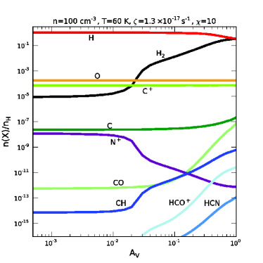
In Figure 4, we present the fractional abundance of several species calculated in a plane-parallel PDR model with illumination from one side, in order to show in which region the species of interest (Table 3.1) reside. For the details of treatment of chemical reactions, etc., see Morata & Herbst (2008). We adopted gas density, $n=100$ cm^-3, gas temperature, $T=60$ K, cosmic-ray ionization rate, $\zeta=1.3\times 10^{-17}$ s^-1, and intensity of the FUV radiation field $\chi=10$ in units of the Draine (1978) standard radiation field. Since we are interested in the diffuse medium, we focus on the regions with $A_{V}\lesssim 1$, where $A_{V}$ is the extinction at $V$ band. Indeed, H₂ dominates the hydrogen species at $A_{V}>1$ as shown in Figure 4 so that molecular clouds are favorably formed at $A_{V}>1$. We observe that both [N ii] and CH are fair THz tracers of the diffuse ISM (note that CO requires a dense state to be excited enough to emit THz lines; Figure 3). Moreover, the excitation energy for the 1.5 THz CH line is $\sim 100$ K, matching the temperature of the cold neutral medium (CNM) (McKee & Ostriker, 1977), outside of molecular clouds. Some other species in Table 3.1 also exist: both HCO⁺ and HCN favor shielded regions and are more suitable for the molecular gas tracer.

Figure 4: Fractional abundance of several interesting species in the THz band with respect to the total abundance of hydrogen atoms as a function of the depth into the cloud, indicated by $A_{V}$, in a plane-parallel PDR model with illumination from one side (to the left in the plot). The physical conditions of the PDR model are: gas density, $n=100$ cm^-3, temperature, $T=60$ K, cosmic-ray ionization rate, $\zeta=1.3\times 10^{-17}$ s^-1, and intensity of the FUV radiation field $\chi=10$ in units of the Draine (1978) standard radiation field.

Godard, Falgarone, & Pineau des Forêts (2008) examined the case of turbulent dissipation regions (TDRs) in the CNM instead of PDRs. In TDRs, the above species (CH and HCO⁺) are also key species. The abundances of these species relative to hydrogen is $\sim 10^{-8}$–$10^{-9}$ for CH and $10^{-10}$–$10^{-9}$ for HCO⁺, slightly larger than the above prediction for the PDR.

High-excitation CO lines are tracers of dense regions located near to the ionizing source. Indeed, Pérez-Beaupuits et al. (2012) observed M17 SW, a giant molecular cloud illuminated by a cluster of OB stars, with the SOFIA/German Receiver for Astronomy at Terahertz (GREAT) and detected the CO $J=13$–12 emission line, which indicates a dense region near to the ionizing source in the nebula. We could probably use THz CO lines to exclude the contamination of dense regions and choose really diffuse regions; that is, we avoid the lines of sights where THz CO lines are detected to choose purely diffuse regions.

In reality observations of other species such as CH and HCO⁺ in emission require much higher sensitivity than those species with strong lines such as CO and [N ii]. If we assume a similar level of intensity to other weak THz lines detected by Herschel ($\sim 0.3$ K), $\sim 100$ hr integration on source would be necessary for a 3 $\sigma$ detection. Therefore, it is recommended that we first observe lines easier to detect such as [N ii] 205 $\mu$m (Section 3.1.3) in the first generation ground-based THz detectors. Alternatively, we observe bright background continuum sources and try to detect the THz lines of minor species in absorption (Gerin et al., 2012).

3.1.3 The diffuse ISM: [N II] 205 $\mu$m

Since the ionization potential of nytrogen (14.5 eV) slightly exceeds 1 Ryd, [N ii] lines trace the ionized medium. In star-forming regions or star-forming galaxies, H ii regions are prevalent because young massive stars emit a large amount of ionizing photons. Indeed, hydrogen recombination lines emitted from H ii regions are often used as indicators of star formation activity (e.g., Kennicutt, 1998).

Recently, Inoue et al. (2014b) have investigated possibilities of using FIR (THz) nebular lines as a tracer of star-forming galaxies. Indeed, FIR fine-structure lines could be a useful star formation indicator of high-redshift galaxies, since ALMA is capable of detecting redshifted FIR fine-structure lines (e.g., Nagao et al., 2012). Because of the small Einstein coefficients, FIR fine-structure lines are usually optically thin. They expressed the line luminosity, $L_{\mathrm{line}}$, as a function of star formation rate (SFR):

$$L_{\mathrm{line}}=C_{\mathrm{line}}(Z,\,U,\,n_{\mathrm{H}})\,\mathrm{SFR},$$ (1)

where $C_{\mathrm{line}}$ is the proportionality constant that depends on the metallicity $Z$, ionization parameter $U$, and hydrogen number density $n_{\mathrm{H}}$. They calculated $C_{\mathrm{line}}$ using the photoionization code cloudy (Ferland et al., 2013) and calibrated the values of $U$ and $n_{\mathrm{H}}$ by comparing with [O iii] 88 $\mu$m line luminosities of nearby galaxies. As a consequence they obtained the values of $C_{\mathrm{line}}$ as a function of metallicity.

Among the lines, [N ii] 205 $\micron$ at redshift 0 can be observed from the ground in the 1.5 THz atmospheric window. Thus, we are able to examine the applicability of [N ii] 205 $\mu$m line strength to the SFR estimate by observing Galactic H ii regions. The critical density of this transition is only 44 cm^-3 at 8000 K (Oberst et al., 2006), so that the collisional excitation is efficient enough. However, the small critical density also means that the [N ii] 205 $\mu$m line is more weighted for the diffuse regions; thus, we keep in mind that, when we compare the [N ii] 205 $\mu$m line with other star-formation indicators in a resolved star-forming regions, the correlation may not be good in dense star-forming regions (Wu et al., 2015). Indeed, Wu et al. (2015) showed, using spatially resolved [N ii] 205 $\mu$m data of M83 taken by Herschel, that the [N ii] intensity has a much shallower dependence on the SFR surface density than expected from a linear relation. They interpret this shallow dependence as the [N ii] emission being more diffuse than other star formation indicators.

On an entire-galaxy scale, at least, the [N ii] 205 $\mu$m emission is potentially a good star-formation indicator (Zhao et al., 2013). Zhao et al. (2013) examined the relation between the [N ii] 205 $\mu$m line luminosity observed in nearby starburst galaxies and their FIR luminosity, which is known to be a good indicator of SFR (e.g., Kennicutt, 1998; Inoue, Hirashita, & Kamaya, 2000). They excluded galaxies with significant contributions from AGNs and included normal star-forming galaxies, for which the [N ii] 122 $\mu$m luminosities are observed by ISO (Brauher, Dale, & Helou, 2008), after converting the [N ii] 122 $\mu$m luminosity to the [N ii] 205 $\mu$m luminosity using the theoretical ratio. As a consequence, they found that there is a tight relation between the [N ii] 205 $\mu$m luminosity and the FIR luminosity:

$$\log\mathrm{SFR}~{}(M_{\odot}~{}\mathrm{yr}^{-1}) = (-5.31\pm 0.32)$$ (2)

$$+(0.95\pm 0.05)\log L_{\mathrm{N\,II}}~{}(L_{\odot}),$$

which is consistent with a linear relation with $C_{\mathrm{NII}}=10^{5.31\pm 0.32}~{}L_{\odot}/(M_{\odot}~{}\mathrm{yr}^{-1})$ (equation 1; when we consider the [N ii] 205 $\mu$m line, we denote $C_{\mathrm{line}}$ as $C_{\mathrm{N\,II}}$). Wu et al. (2015) also show the integrated [N ii] 205 $\mu$m luminosity and SFR of M83 matches this relation. Inoue et al. (2014b) derived $C_{\mathrm{N\,II}}=10^{6.23}$ and $10^{5.48}~{}L_{\odot}/(M_{\odot}~{}\mathrm{yr}^{-1})$ for 1 $Z_{\odot}$ and 0.4 $Z_{\odot}$, respectively. Since equation (2) is derived for bright galaxies, the metallicity is probably nearly solar. If the metallicity is solar, Inoue et al. (2014b) tends to overproduce $C_{\mathrm{N\,II}}$. To examine this possible discrepancy, further tests are necessary with a fixed-metallicity sample. We propose the following tests using Galactic H ii regions, whose metallicities can be assumed to be solar.

A representative indicator of SFR (or H ii regions) is H$\alpha$ emission (e.g., Kennicutt, 1998), which is linked to the SFR under the solar metallicity and the same initial mass function (IMF) as adopted by Inoue et al. (2014b) by the following equation (Hirashita, Buat, & Inoue, 2003):

$$\mathrm{SFR}=C_{\mathrm{H\alpha}}L_{\mathrm{H\alpha}}^{\mathrm{c}},$$ (3)

where $C_{\mathrm{H\alpha}}=7.9\times 10^{-42}(\mathrm{M}_{\odot}~{}\mathrm{yr}^{-1})/(\mathrm{erg~{}s}^{-1})$, and $L_{\mathrm{H\alpha}}^{\mathrm{c}}$ is the H$\alpha$ luminosity corrected for extinction.

Inserting equation (3) into equation (1), we obtain

$$L_{\mathrm{N\,II}}=C_{\mathrm{H\alpha,N\,II}}L_{\mathrm{H\alpha}}^{\mathrm{c}},$$ (4)

where $C_{\mathrm{H\alpha,N\,II}}\equiv C_{\mathrm{N\,II}}\,C_{\mathrm{H\alpha}}.$ (As we noted above, we denote $C_{\mathrm{line}}$ for the [N ii] 205 $\mu$m emission as $C_{\mathrm{N\,II}}$.) For the [N ii] 205 $\mu$m line, Inoue et al. (2014b) obtained $C_{\mathrm{N\,II}}(Z,\,U,\,n_{\mathrm{H}})=10^{39.82}$ (erg s^-1)/(M_⊙ yr^-1) for the solar metallicity, by adopting $\log U=-3$ and $\log n=1$. In this case, $C_{\mathrm{H\alpha,N\,II}}=0.0521$.

Equation (4) can be checked or calibrated with a sample of Galactic H ii regions whose H$\alpha$ luminosities are already measured. Note that the proportionality constant does not change even if we use the surface brightness, i.e., $I_{\mathrm{N\,II}}=C_{\mathrm{H\alpha,N\,II}}I_{\mathrm{H\alpha}}^{\mathrm{c}}$.

The major disadvantage of H$\alpha$ line is that H$\alpha$ photons are subject to dust extinction. A way of resolving this problem is that the extinguished portion of the H$\alpha$ luminosity is corrected using the FIR dust emission (Kennicutt et al., 2007). Alternatively, radio free–free emission, which is free from dust extinction, can also be used as a tracer of H ii region, although contamination with synchrotron or dust radiation might be a problem depending on the frequencies. Mezger, Smith, & Churchwell (1974) relate the radio free–free flux $S_{\nu}$ to the number of ionizing photons radiated per time $N_{\mathrm{Lyc}}$ (referred to as ionizing photon luminosity) as

$$N_{\mathrm{Lyc}} = 4.8\times 10^{48}a(\nu,\,T_{e})^{-1}\left(\frac{\nu}{\mathrm{GHz}}\right)^{0.1}\left(\frac{T_{e}}{\mathrm{K}}\right)^{-0.45}$$ (5)

$$\times\left(\frac{S_{\nu}}{\mathrm{Jy}}\right)\left(\frac{D}{\mathrm{kpc}}\right)^{2}~{}\mathrm{s}^{-1},$$

where $a(\nu,\,T)$ is a slowly varying function, which is assumed to be 1 for the electron temperatures of interest ($T_{e}\sim 10^{4}$ K), and $D$ is the distance to the object. Using the relation $(N_{\mathrm{Lyc}}/\mathrm{s}^{-1})=7.3\times 10^{11}[L_{\mathrm{H\alpha}}/(\mathrm{erg~{}s^{-1}})]$ (Deharveng et al., 2001), the above equation is equivalent with

$$L_{\mathrm{H\alpha}}^{\mathrm{c}} = 6.5\times 10^{36}a(\nu,\,T_{e})^{-1}\left(\frac{\nu}{\mathrm{GHz}}\right)^{0.1}\left(\frac{T_{e}}{\mathrm{K}}\right)^{-0.45}$$ (6)

$$\times\left(\frac{S_{\nu}}{\mathrm{Jy}}\right)\left(\frac{D}{\mathrm{kpc}}\right)^{2}~{}\mathrm{erg~{}s^{-1}}.$$

Further, using equation (4), we obtain

$$L_{\mathrm{N\,II}} = 6.5\times 10^{36}\,C_{\mathrm{H\alpha,N\,II}}\,a(\nu,\,T_{e})^{-1}\left(\frac{\nu}{\mathrm{GHz}}\right)^{0.1}$$ (7)

$$\times\left(\frac{T_{e}}{\mathrm{K}}\right)^{-0.45}\left(\frac{S_{\nu}}{\mathrm{Jy}}\right)\left(\frac{D}{\mathrm{kpc}}\right)^{2}~{}\mathrm{erg~{}s^{-1}}.$$

The expected flux of [N ii] 205 $\mu$m, $f_{\mathrm{N\,II}}$ is then

$$f_{\mathrm{N\,II}} = \frac{L_{\mathrm{N\,II}}}{4\pi D^{2}\Delta\nu}$$ (8)

$$= 5.4\times 10^{7}\,C_{\mathrm{H\alpha,NII}}\,a(\nu,\,T_{e})^{-1}\left(\frac{\nu}{\mathrm{GHz}}\right)^{0.1}$$

$$\times\left(\frac{T_{e}}{\mathrm{K}}\right)^{-0.45}\left(\frac{S_{\nu}}{\mathrm{Jy}}\right)\left(\frac{\Delta\nu}{10^{8}~{}\mathrm{Hz}}\right)^{-1}~{}\mathrm{Jy},$$

where $\Delta\nu$ is the assumed frequency width of the line ($10^{8}$ Hz corresponds to a velocity width of 20 km s^-1 at 1.5 THz). Here we assume that the instrumental frequency resolution is smaller than the physical broadening of the line. By adopting $a(\nu,\,T_{e})=1$, and taking the normalization at $\nu=5$ GHz (wavelength 6 cm, as we use later) and $T_{e}=10^{4}$ K, the above equation is reduced to

$$f_{\mathrm{N\,II}} = 1.0\times 10^{6}\,C_{\mathrm{H\alpha,NII}}\,\left(\frac{\nu}{5~{}\mathrm{GHz}}\right)^{0.1}\left(\frac{T_{e}}{10^{4}~{}\mathrm{K}}\right)^{-0.45}$$ (9)

$$\times\left(\frac{S_{\nu}}{\mathrm{Jy}}\right)\left(\frac{\Delta\nu}{10^{8}~{}\mathrm{Hz}}\right)^{-1}~{}\mathrm{Jy}.$$

Galactic H ii regions to be observed by the GLT (Mathis, 2000) Name $(l,\,b)\,^{\mathrm{a}}$ $\alpha$(J2000) $\delta$(J2000) Size^b $S_{\nu}$(6 cm) $f_{\mathrm{N\,II}}\,^{\mathrm{c}}$ $f_{\mathrm{N\,II,\,beam}}\,^{\mathrm{d}}$ (h m s) (  ) (Jy) (MJy) (Jy/beam) W 3 133.7+1.2 02 25 30 +62 05 19 $1\farcm 7\times 1\farcm 5$ 80 0.38 420 W 51 49.5$-$0.4 19 23 48 +14 30 46 complex 400 – – DR 21 81.7+0.5 20 39 15 +42 19 11 $0\farcm 3\times 0\farcm 4$ 19 0.090 2400 NGC 7538 111.5+0.8 23 13 21 +61 28 32 $2\farcm 3\times 1\farcm 9$ 26 0.12 90 ^aGalactic coordinate.
^bSize in the directions of $\alpha$ and $\delta$.
^c[N ii] 205 $\mu$m flux estimated by $f_{\mathrm{N\,II}}=4.7\times 10^{3}(S_{\nu}/\mathrm{Jy})$ Jy, which is derived with $C_{\mathrm{H\alpha,N\,II}}=4.0\times 10^{-3}$ and $T_{e}=7,000$ K (these values are appropriate for Carina I and Carina II) in equation (9).
^d[N ii] 205 $\mu$m flux per beam, where the beam size is assumed to be $4^{\prime\prime}\times 4^{\prime\prime}$.

It is possible to calibrate $C_{\mathrm{H\alpha,NII}}$ with Galactic H ii regions. Ground-based observations of [N ii] 205 $\mu$m were already performed for the Carina Nebula by Oberst et al. (2011) with the South Pole Imaging Fabry-Perot Interferometer (SPIFI) at the Antarctic Submillimeter Telescope and Remote Observatory (AST/RO). The beam size was 54^′′ FWHM. For Carina I and Carina II, they obtained [N ii] 205 $\mu$m brightness of $1.87\times 10^{-7}$ and $1.62\times 10^{-7}$ W m^-2 sr^-1, respectively. Multiplying the intensity with the consistent area with radio observations by Huchtmeier & Day (1975), that is, $4\farcm 5\times 6\farcm 3$ and $5\farcm 2\times 4\farcm 8$ for Carina I and Carina II, respectively, we obtain $F_{\mathrm{NII}}=3.5\times 10^{-10}$ and $2.7\times 10^{-10}$ erg s^-1 cm^-2, respectively, where $F_{\mathrm{N\,II}}$ is the integrated flux over all the frequency range (i.e., $F_{\mathrm{N\,II}}=f_{\mathrm{N\,II}}\Delta\nu$). Huchtmeier & Day (1975) obtained 70.2 and 53.7 Jy at 8.87 GHz for Carina I and Carina II, respectively. By adopting $\nu=8.87$ GHz and $T_{e}=7000$ K (Huchtmeier & Day, 1975) in equation (9), we obtain $C_{\mathrm{H\alpha,NII}}=4.0\times 10^{-3}$ for both Carina I and Carina II. This is an order of magnitude smaller than the value above obtained based on Inoue et al. (2014b) (0.0521), probably because of the different values of $U$ and $n$. Indeed, the [N ii] 205 $\mu$m intensity is sensitive to those quantities; for example, a larger value of $n$ or a larger value of $U$ appropriate for the Carina Nebula significantly reduces the [N ii] 205 $\mu$m intensity (e.g., Nagao et al., 2012). It is interesting to point out that we obtained the same value of $C_{\mathrm{H\alpha,NII}}$ for both Carina I and Carina II; indeed, Oberst et al. (2011) show that they have similar gas density and radiation field intensity from line ratio analysis (see their figure 17).

A larger sample taken by the GLT would help to derive more general conclusions for $C_{\mathrm{H\alpha,NII}}$ for the solar metallicity environments. In Table 3.1.3, we list representative Galactic H ii regions whose declination ($\delta$) is larger than 12^∘. The sample is taken from Mathis (2000). Observations of these objects provide a local calibration of [N ii] 205 $\mu$m luminosity as an indicator of star formation rate. Using the sensitivity discussed in Section 2.3, we estimate the on-source integration time necessary to detect the faintest H ii region in Table 3.1.3 (NGC 7538) with 5$\sigma$ as 13 min with a spectroscopic resolution of 2 km s^-1. Because of the extended nature of H ii regions, a multi-pixel detector is desirable.

Metallicity dependence of [N ii] emission is addressed by observing nearby galaxies (Cormier et al., 2015). In fact, the high angular resolution of the GLT is useful for resolving or separating extragalactic H ii regions (Section 3.3.2). With these efforts for [N ii] 205 $\mu$m observations of nearby objects, we will be able to provide a firm local calibration of FIR fine-structure lines as a star-formation indicator. As mentioned above, fine-structure lines are already used as a star formation indicators accessible from ALMA bands for high-redshift galaxies.

3.2 Dust continuum

3.2.1 Importance of THz bands

To derive the dust temperature, we need two or more bands in the FIR. In the wavelength range where dust emission dominates, angular resolution comparable to GLT THz observations can only be achieved by submm interferometers or Herschel PACS at its shortest wavelength $\sim 70~{}\mu$m ($\sim 6^{\prime\prime}$; Foyle et al. 2012). The emission at such a short wavelength as 70 $\mu$m is contaminated by very small grains which are not in radiative equilibrium with the interstellar radiation field (Draine & Anderson, 1985). Thus, the combination of THz observations by GLT with interferometric submm observations is the best way to make dust temperature maps in galaxies.

Here we examine how useful adding 1.5 THz data is to determine the dust temperature. To quantify the goodness of dust temperature estimate, we carry out a simulation by the following steps (see Appendix for details): First, we give a certain dust temperature ($T_{\mathrm{real}}$) and produce observed flux at given wavelengths by adding noise, which mimics the observational error. Next, we fit the data and determine the dust temperature $T_{\mathrm{obs}}$, which is compared with $T_{\mathrm{real}}$. The results are summarized as follows:

1. Addition of THz data to submm data improves the dust temperature estimate, especially for the range of dust temperatures ($\lesssim$30 K) typical of nearby galaxies (Figure 15). In particular, with only submm bands, 450 $\mu$m and 850 $\mu$m, the error of dust temperature is larger than the dust temperature itself at $>20$ K even if the flux uncertainty is less than 30%. (Figure 16). A shorter wavelength (i.e., $\sim 200~{}\mu$m; 1.5 THz), nearer to the peak of dust SED, is better than a longer wavelength (i.e., $\sim 300~{}\mu$m; 1 THz).

2. If we only use THz bands, 200 and 300 $\mu$m, the temperature estimate is not as good as in the case of having submm data points as well (compare Figures 15a and d). This is because these two bands are so close that the temperature estimate is not robust against the errors in the flux measurements. If we only use the THz windows for the dust temperature estimates, the measurement error should be smaller than 10% (Figure 17).

3. If submm measurements are precise such that the error is within 3%, the dust temperature is determined quite well without THz data (20% error in the dust temperature at $<$40 K; Figure 16). However, addition of a THz data point, if the THz measurement error is within 10%, actually improves a temperature significantly, especially at $T_{\mathrm{dust}}\gtrsim 40$ K (Figure 16), and the error of the dust temperature is suppressed to $\sim$10% even at 50 K. Such a temperature is of significant importance to actively star-forming regions/galaxies (e.g., Hirashita et al., 2008).

3.2.2 Continuum observations of star-forming regions: filamentary molecular cluods and their structures

Figure 5: Hierarchical fragmentation suggested in the Orion Giant Molecular Cloud A. Left panel: The 850 $\mu$m continuum image obtained with the SMA (color) overlaid with the continuum at same wavelength obtained with the JCMT (white contours; Johnstone & Bally 1999). Black open circles present clumps identified by JCMT observations, in which the reported clumps line up along the filaments with a spacing of $\sim$0.3 pc (Takahashi et al., 2013). Pink open circles present identified individual star forming sites with the SMA (Takahashi et al., 2013). The average separation of between detected sources are $\sim$0.05 pc. Black filled circles in the bottom right corner show the JCMT and SMA beam sizes of 14$\arcsec$ and $4\farcs 5$, respectively. At the distance of the cloud (414 pc; Menten et al. 2007), $1^{\prime}$ corresponds to 0.12 pc. Right panel: Observed separations of clouds/clumps/cores as a function of the mean number density of the parental cloud. The filled circles show the separation with $i=90^{\circ}$ (filament is in the plane of the sky), and the open circles show the separation with $i=30^{\circ}$ (filament closer to being perpendicular to the plane of the sky). The doted line shows the best fit of the observed results (power law index of $-1.4$). The solid lines with various colors show expected maximum instability size derived from Jeans length calculation with various temperatures indicated in the small panel. The size scale achieved by the GLT angular resolution at THz ($\sim 4\farcs 0$ or 0.008 pc at the distance of the Orion cloud, 414 pc) is indicated by an arrow in the upper part of the horizontal axis. The size scale which can be mapped with the GLT is highlighted in blue.

How the ISM structures change associated with star formation processes should provide a key to the dominant physical processes of star formation. It has been known that parsec-scale filamentary structures are common for molecular clouds (e.g., Schneider & Elmegreen, 1979; Myers, 2009). Recent Herschel observations have revealed the ubiquity of such filamentary structures both in low- and high-mass star-forming regions with a high dynamic range in mass (André et al., 2010; Könyves et al., 2010; Arzoumanian et al., 2011; Hill et al., 2012). These filamentary molecular clouds often show hierarchical structures and fragment into $\sim$0.1 pc scale clumps, which likely corresponds to coherent-velocity filaments and isothermal cores (Pineda et al., 2010; Hacar et al., 2013). They will presumably fragment into star-forming cores. Therefore, multi-scale fragmentation processes are likely a key process that determines the prestellar and protostellar core mass function, which may directly lead to the stellar initial mass function. Here we examine a possibility of tracing the ISM structures associated with the star formation processes by the continuum emission.

Previous studies suggest that observations of low-mass-star-forming regions are consistent with thermal Jeans fragmentation (Alves, Lombardi, & Lada, 2007), while observations of massive-star-forming regions are better described by turbulent fragmentation (Pillai et al., 2011). Recent interferometric observations have started to spatially resolve the individual star-forming sites and suggested multi-scale periodical structures within filaments toward several different regions (Zhang et al., 2009; Wang et al., 2011; Liu et al., 2012; Takahashi et al., 2013; Wang et al., 2014).

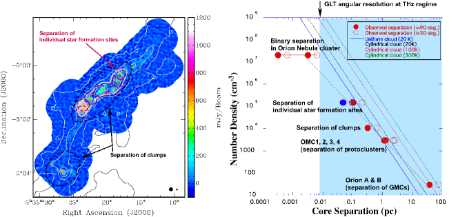
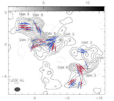
As an example, Takahashi et al. (2013) detected quasi-periodical separations between sources with a spacing of $\sim$0.05 pc in the Orion Molecular Cloud-3 region (OMC-3; Figure 5). This spatial distribution is part of a larger hierarchical structure, which also includes fragmentation scales of GMCs ($\simeq$37 pc), representative star forming regions of OMC-1, -2, -3, and -4 ($\simeq$1.3 pc), and clumps ($\simeq$0.3 pc). This suggests that hierarchical fragmentation operates within the OMC regions. The measured separations of GMCs and representative star-forming regions are larger than those expected from the thermal fragmentation length, suggesting turbulent dominant fragmentation. The measured separations of clumps are comparable to the thermal fragmentation length, and those of spatially resolved individual cores are smaller than those expected from the thermal fragmentation length, which could be explained by local collapse within the clumps (gravitational focusing of the edges of the elongated structure) or helical magnetic fields. These results imply that the multi-scale turbulent dissipation and consequent fragmentation processes may play an essential role in determining the initial physical condition of cores and the census of filamentary molecular clouds. Furthermore, SMA 1.3 mm continuum observations toward OMC-1n, which is located $\simeq$2.2pc south from OMC-3 and connected to the most massive part of the cloud OMC-1, show a double peaked distribution of the source separations, corresponding to quasi-equidistant lengths of $\sim$0.06 pc for the clumps and 0.012 pc for the individual star-forming cores (Teixeira et al., 2015). Comparison between OMC-3 and OMC-1n clearly demonstrates that the source separation varies along the OMC filaments. This suggests that the initial condition of cores and their census could vary within the parsec-scale filamentary molecular clouds.

Sampling individual star-forming sites, which typically have a size of $\leq$0.1 pc (Figure 5) and are mainly observed with the (sub)mm interferometers, is limited by targeted observations. On the other hand, imaging of parsec-scale clouds are mainly performed by ground-based single-dish (sub)mm telescopes or space infrared telescopes. These single dish facilities are not able to spatially resolve individual star-forming sites except the nearest low-mass star-forming regions ($\sim$150 pc). Thus, it has been difficult to study multi-scale structures in filamentary molecular clouds systematically with a uniform data set.

The GLT, with its typical resolution of 4(Section 2.3), will be able to resolve individual star formation sites up to distances of $\sim$500 pc. THz observations will have an advantage of observing continuum emission originating from prestellar cores and T Tauri sources at the wavelengths close to their SED peaks. Multi-wavelength continuum detectors anticipated to be onboard the GLT enable us to directly measure dust temperature and dust emissivity within filamentary molecular clouds such as demonstrated by the recent SCUBA-2 observations (Hatchell et al., 2013; Rumble et al., 2015; Salji et al., 2015). As discussed in Section 3.2.1, adding THz observations to existing data sets will help us to estimate those quantities more precisely. Estimated dust temperatures will be directly used for estimating the thermal fragmentation lengths, which will be compared with the separations of spatially resolved sources. This will tell us what kind of fragmentation process is dominant on each size scale and in different parts of a filament. Moreover, the correct dust temperature serves to obtain a good estimate of the total dust mass (or the total gas mass with an assumption of dust-to-gas ratio), which is crucial to study the census of filamentary molecular clouds.

The SMA observations by Takahashi et al. (2013) had a similar beam size to the GLT. The peak brightnesses that they detected were in the range of $\sim 100$–4000 mJy beam^-1. If we assume a power-law spectrum expected for the Rayleigh-Jeans side of the SED with an index of $\alpha=2.5$, we obtain $(1500/350)^{2.5}$ times 100 mJy beam^-1 for the faintest case, i.e., 3.8 Jy beam^-1. Aiming at a root mean square (rms) of 0.4 Jy beam^-1 ($\sim 10\sigma$ detection for the peak), a source requires an on-source integration time of 34 min (Section 2.3). Currently the specs for THz bolometers to be equipped on the GLT are not clear yet. However, if we assume the similar spec as ArTeMiS (Architectures de bolometres pour des Telescopes a grand champ de vue dans le domaine sub-Millimetrique au Sol) equipped on APEX has at 350 $\mu$m (Revéret et al., 2014), the field of view (FOV) of bolometer will be expected as $\sim 5\farcm 0\times 2\farcm 5$. Assuming the same FOV, mapping of a GMC which has a similar angular size to the northern part of the Orion A molecular cloud of $\sim 35^{\prime}\times 75^{\prime}$ (Salji et al., 2015) retuires 210 mosaic images. As estimated above, the on-source time on each FOV is 34 min; thus, naive estimation of the total on-source observing time would be 34 min $\times$ 210 = 119 hr.

3.2.3 Importance for polarization studies

Polarization continuum observations in the THz frequency range are an unexplored domain. Dust continuum emission peaks at THz frequencies. Lower frequency observations in the submm regime by the JCMT at 850 $\micron$ (e.g., Matthews et al., 2009), the Caltech Submillimeter Observatory (CSO) at 350 $\micron$ (e.g., Dotson et al., 2010), the SMA at 870 $\micron$ (e.g., Rao et al., 2009; Tang et al., 2010; Zhang et al., 2014) and CARMA at 1.3 mm (e.g., Hull et al., 2014) reveal typically dust polarized emission at a level of a few percent up to about 10% of Stokes $I$. The dust continuum polarized emission is thought to result from dust particles being aligned with their shorter axes parallel to the magnetic field (e.g., Hildebrand et al., 2000; Lazarian & Hoang, 2007). The magnetic field is being recognized as a key component in star formation theories (e.g., McKee & Ostriker, 2009). Polarization observations toward star-forming regions provide, therefore, a unique tool to map the sky-projected magnetic field morphology.

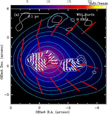
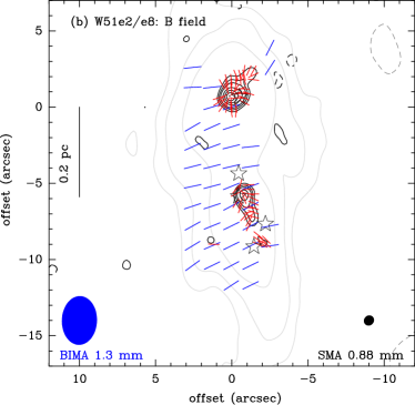
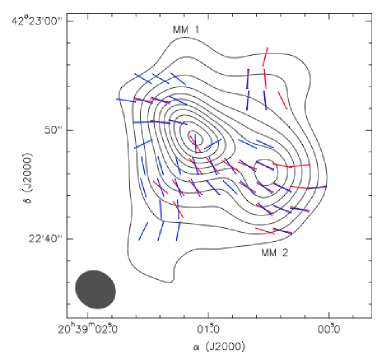
Unlike the, so far, rather isolated Zeeman effect observations, dust polarization observations can yield coherent magnetic field structures over an extended area. Recent observations with the SMA (e.g., Girart et al., 2006, 2009; Tang et al., 2009, 2013; Qiu et al., 2013) are revealing hourglass-like magnetic field structures in collapsing cores. These high-resolution observations ($\sim 0.7\arcsec$) in combination with new analysis tools (Koch et al., 2012, 2013, 2014) are now leading to new insights into the role of the magnetic field in the star-formation process. At the same time, these observations also show that it is crucial to not only resolve the field structures in the collapsing cores, but that it is equally important to trace the magnetic field at intermediate scales ($\sim 2$–$5\arcsec$) in order to fully understand the role of the field in star formation across all scales (Figure 6, upper panel). These intermediate scales – in contrast to the large scales ($\sim 10$–$20\arcsec$) traced by the JCMT and CSO – often reveal the structure of the core-surrounding envelope. Consequently, they provide information on how the material is transported close to the cores before a collapse is initiated. Figure 6 (upper panel) illustrates this for W51 North where the magnetic field in the envelope appears to channel material that leads to the formation of denser cores along a central axis. The filamentary envelope around W51 e2/e8 (Figure 6, lower panel) is another example where a uniform field morphology (from a resolution of about $3\arcsec$; Lai et al. 2001) perpendicular to the filament’s major axis is likely guiding and defining the locations of the denser collapsing cores e2 and e8 (Tang et al., 2009). The high-mass star-forming region DR21(OH) displays a fragmentary structure when observed with the SMA with a resolution of about $0.7\arcsec$ (Girart et al., 2013). Zooming out shows again more coherent and regular field patterns in its sourrounding environment (Figure 7). Thus, THz observations with a 12-m single-dish antenna, providing resolutions around $\sim 4\arcsec$, will ideally sample these envelope scales. Moreover, these scales will be probed without the zero-spacing missing flux that is present in an interferometer like e.g., the SMA.

Figure 6: (a): SMA dust polarization observation at 870 $\micron$ (345 GHz) toward the star forming region W51 North (Tang et al., 2013). The color coding and gray contours are the Stokes $I$ dust continuum emission from subcompact (synthesized beam resolution $\sim 4\arcsec$) and extended ($\sim 0\farcs 7$) array configurations, respectively. The corresponding magnetic field orientations are shown with red and white segments, respectively. The 4$\arcsec$ resolution observation seems to trace the envelope of the collapsing higher-resolution cores, with the magnetic field channeling material from both the north and south leading to the formation of cores along an east-west axis. (b): Reproduced based on Tang et al. (2009). The filamentary structure observed by the Berkeley-Illinois-Maryland Association (BIMA) array with $\sim 3\arcsec$ resolution from Lai et al. (2001) around W51 e2/e8 with dust continuum in gray contours. The magnetic field is shown with blue segments mostly perpendicular to the filament’s longer axis. The SMA higher resolution observations ($\sim 0\farcs 7$ resolution) resolve the two cores e2 and e8 (dust continuum intensity in black contours and magnetic field in red segments) that probably appear at locations defined by the larger scale field and filament. The synthesized beam resolutions are shown in the lower-left and lower-right corners. The stars mark ultracompact H ii regions.

Figure 7: Upper panel: DR21(OH) dust continuum contours observed with the SMA and convolved with a $\sim 3\arcsec$ resolution to match earlier BIMA observations from Lai et al. (2003). Magnetic field segments from the SMA and BIMA are in blue and red, respectively. Lower panel: The SMA higher resolution observations ($\sim 0.7\arcsec$ resolution) zooming in onto MM 1 and MM 2 from the upper panel. Highly fragmented structures become apparent. Contours display the dust continuum and magnetic field segments in red and blue are detections at more than $3\sigma$ and between 2.5–3$\sigma$. Figures are reproduced from Girart et al. (2013).

Yet another relatively unexplored topic in dust polarization studies is the role of different dust grain populations as they presumably exist in different shapes, sizes, and compositions. Typically, it is assumed that dust particles are aligned with their shorter axes parallel to the magnetic field, so that detected polarization orientations rotated by 90^∘ reveal the magnetic field morphology (Cudlip et al., 1982; Hildebrand et al., 1984; Hildebrand, 1988; Lazarian & Hoang, 2007; Andersson, 2012). Although this is the common practice, this only reflects a crude picture of a “universal” dust grain presumably coupling to the magnetic field while a lot of detailed dust physics is left out. Dust polarized emission is generally thought to be a complex function of many parameters like dust size and shape, dust populations with different temperatures, dust paramagnetic properties, external magnetic field etc. (e.g., Lazarian, 2007). Current dust polarization observations in the submm regime are typically limited to one observing frequency at a telescope, which necessarily limits information, sampling likely only a certain population of dust particles. Combining dust polarization observations from several frequencies can shed light on the composition of dust populations.

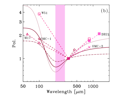
Recent studies by Vaillancourt & Matthews (2012) comparing polarization percentages and polarization position angles between JCMT 850 $\mu$m and CSO 350 $\mu$m sources provide hints for mixtures of different grain properties and polarization efficiencies. In the densest part of molecular cloud cores, the polarization spectrum rises monotonically with wavelength (Vaillancourt, 2011), which is consistent with the effect of optical depth. In cloud envelopes, where the FIR–submm emission is optically thin, the polization spectrum falls with wavelength up to $\sim 350~{}\mu$m, while it rises at longer wavelengths (Figure 8). This non-monotonic behavior requires multiple components whose polarization degrees are correlated with the dust temperature and/or spectral index (Hildebrand et al., 1999; Vaillancourt, 2011).

For more quantification of the importance of THz observations, we adopt an empirical multi-component SED–polarization model in Hildebrand et al. (1999) and Vaillancourt (2002). If the emitting dust consists of components with different emission and polarization properties, the resulting polarization spectrum, $P_{\mathrm{tot}}(\lambda)$, is estimated as a flux-weighted average of each component:

$$P_{\nu,\mathrm{tot}}=\sum_{i}p_{i}X_{i}(\lambda),$$ (10)

where $i$ is the index of the components, $p_{i}$ is the polarization degree of component $i$, and $X_{i}(\lambda)$ is the ratio of the flux at wavelength $\lambda$ given by $X_{i}(\lambda)\equiv F_{\nu,i}(\lambda)/F_{\nu,\mathrm{tot}}(\lambda)$ with $F_{\nu,i}(\lambda)$ being the flux density emitted by component $i$ and $F_{\nu,\mathrm{tot}}(\lambda)\equiv\sum_{i}F_{\nu,i}(\lambda)$. The flux, $F_{\nu,i}(\lambda)$, is assumed to be described by a modified black body with an emissivity index of $\beta_{i}$:

$$F_{\nu,i}(\lambda)=W_{i}\nu^{\beta_{i}}B_{\nu}(T_{i}),$$ (11)

where $B_{\nu}(T_{i})$ is the Planck function at frequency $\nu$ and temperature $T_{i}$ and $W_{i}$ describes the weight for the component $i$.

For the purpose of showing representative examples, we first adopt the same parameters as in Vaillancourt (2011). We examine two models: one is a two-component model in which $\beta_{i}$ is different between the two components ($\beta_{1}=1$ and $\beta_{2}=2$), while the other is a three-component model in which $\beta_{i}$ is the same ($\beta_{i}=2$) for all the three components ($i=1$, 2, and 3). Each component has a different dust temperature, 45, 17, and 10 K for $i=1$, 2, and 3, respectively, and a different polarization degree, $p_{i}=4$, 0, and 3 for $i=1$, 2, and 3, respectively (the last component does not exist in the two-component model). In this analysis we are only interested in the relative strength of polarization, and the polarization is always normalized to the value at 350 $\micron$ (this is why we give $p_{i}$ without units). In Figure 8, we show the results for the polarization spectrum ($P_{\nu,\mathrm{tot}}(\lambda)$) and the flux ($F_{\nu,i}(\lambda)$ and $F_{\nu,\mathrm{tot}}$) for these typical choices of values given in Vaillancourt (2011). The flux is normalized so that the maximum of $F_{\nu,\mathrm{tot}}$ is 1.

Figure 8: Upper windows in each panel: Polarization spectra calculated by the models in the text, compared with measured polarization spectra for molecular cloud envelopes, normalized at 350 $\micron$. The observational data are taken from Vaillancourt et al. (2008) and references therein. Data at 850 $\micron$ are from the JCTM. The wavelength range between 100 and 350$\micron$ is unexplored. Lower windows in each panel: Corresponding SEDs. The solid line is the total (the peak is normalized to 1) and the components are shown by dotted, dashed, and dot-dashed lines. The shaded regions in the upper and lower panels show the THz coverage expected for the GLT. Panel (a): A 2-temperature component SED with $T_{1,2}=45$ and 17 K, $\beta_{1,2}=1$ and 2, and $p_{1,2}=4$ and 0%. Panel (b): A 3-temperature component SED with $T_{1,2,3}$= 45, 17 and 10 K, $\beta_{1,2,3}=2$, 2, and 2, and $p_{1,2,3}=4$, 0, and 3 (only the relative polarization strangths among the components are important). Differences and changes in slopes are apparent at $\sim$100–300 $\micron$.

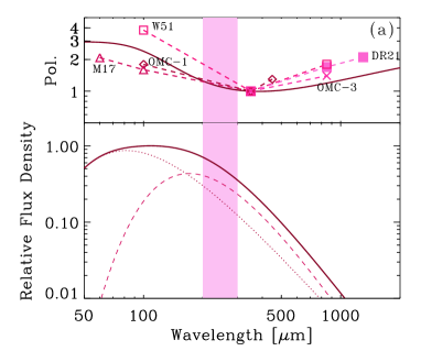
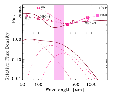
As shown in Figure 8, we confirm the previous results that the non-monotonic behavior of the polarized spectrum is reproduced both by the 2- and 3-component models. The observational studies are currently limited to a few wavelengths with no observations in the THz atmospheric window (1–1.5 THz) regime (Figure 8). The falling spectrum between 60 and 350 $\micron$ is indicative of a dust model where warmer grains are better aligned than colder grains (Hildebrand et al., 1999; Vaillancourt, 2002). The change in slope with the rising spectrum at $\geq 350~{}\micron$ requires a second dust component with a colder temperature or a lower spectral index than the warmer component. Generally, a varying polarization spectrum will require at least 2 dust components at different temperatures. Every change from a falling to a rising (or vice versa) spectrum and every (noticeable) change in the slope will point toward an additional component. Measurements in the THz regime around 200 $\mu$m will fill in the gap between 100 and 350 $\mu$m which can distinguish between a 2-temperature and a 3-temperature component model (Figure 8). Additionally, in combination with ALMA, which is expected to eventually cover polarization observations up to about 900 GHz, we will be able to study dust grain polarization properties in the full frequency range around THz.

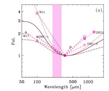
To emphasize more the importance of the GLT THz wavelengths, we present the polarization spectra for various fractions of component $i=2$, which contributes to the flux at THz wavelengths the most, in Figure 9. We observe a clear distinction in the polarization spectra between the 2- and 3-component models. As mentioned above, in the 2-component model, the difference tends to appear at wavelengths out of the range where the contribution of component $i=2$ (with $T=17$ K; i.e., the component peaking at the THz frequencies) to the flux is dominated. In contrast, the 3-component model predicts that the THz polarization is sensitive to the different contribution from component $i=2$. Therefore, adding a data point at THz wavelengths to both the SED and the polarization spctrum provides a strong test for the multi-component dust models. Within the GLT THz band (i.e., the shaded region in Figure 9), the shortest wavelength (i.e., 200 $\mu$m; or frequency 1.5 THz) has the largest advantage in distinguishing the difference given the 350 $\mu$m data, simply because it is the farthest from 350 $\mu$m.

Figure 9: Same as the upper windows in each panel of Figure 8, but for various fractions of the 17-K component (component $i=2$), which contributes to the THz band the most. The solid, dotted, and dot-dashed lines show the same fraction as in Figure 8, an increased fraction of component $i=2$ by a factor of 3, and a decreased fraction of component $i=2$ by a factor of 3, respectively.

Careful modeling of radiative transfer will be an additional asset. The different frequencies possibly sampling different grain populations are likely also presenting different optical depths. By consistently treating the optical depth effects with the temperature variation, a complete frequency coverage including the THz domain will eventually also allows us to do dust polarization tomography with an ultimate goal of understanding the 3-dimensional magnetic field structure.

The polarization capability of the THz detectors discussed in Section 6 is not well established. For the purpose of roughly estimating time and efficiency for a typical continuum polarization observation in the THz regime, we can use a comparison with the SMA that has been conducting polarization observations over the past decade. The GLT, operating at $\lambda\sim 200~{}\mu$m, will win over the SMA ($\lambda\sim 870~{}\mu$m) by a factor $\sim(870/200)^{2.5}\sim 30$, assuming dust emission to scale in frequency with a power-law index $\alpha=2.5$. The GLT will loose in collecting area by a factor 2 as well as in system temperature by a factor of $\sim$100 (Table 1) compared with the SMA. All together, the GLT is likely to be a little slower in integration time than the SMA by a factor $\sim 3$. This further builds on anticipating a multi-beam receiver, covering a field-of-view similar to the SMA ($\sim 30\arcsec$). Currently, the SMA is reaching a $\sim 1$ mJy beam^-1 sensitivity, allowing $\sim 7\sigma$ detection on a typical Galactic source in one night. We, therefore, project similar numbers for the GLT, i.e., 1–2 source detections per night. In order to maximize scientific impact and to be able to perform statistical studies, we are aiming for a dedicated program with a sample of $\sim$50 star-forming regions. Including overhead (e.g., technical issues, bad weather) we expect $\sim 3$ months to carry out such a program.

SOFIA/High-resolution Airborne Wideband Camera (HAWC), which covers 50–240 $\mu$m, also has a capability of THz polarimetry. Since the atmospheric transparency is much better for SOFIA than for the GLT, HAWC has better sensitivity than the GLT. However, the beam size of SOFIA (19$\arcsec$) may be too large to trace the interesting structures shown in Figures 6 and 7.

In summary, the uniqueness of THz dust continuum polarization observations with a 10-m class antenna such as the GLT lies in what follows: We can trace the polarization of the dust component that have the largest contribution to the spectral peak. Compared with airborne and space THz observatories, the ground-based THz telescopes provide higher angular resolutions, which correspond to intermediate scales of a few arcsec in Galactic star-forming regions. THz dust polarization observations will probe different dust grain populations and/or different optical depths from existing submm observations. Thus, adding the THz polarization data point provides additional constraints to separate different dust components. Furthermore, in combination with the SMA and ALMA covering a frequency range up to about 900 GHz, various optical depths or various dust temperature layers will be probed, which will allow us to do dust polarization tomography well into the THz regime.

3.3 Extragalactic THz cases

Dust emission from a galaxy is often used as an indicator of SFR since young massive stars dominate the total stellar light in star-forming galaxies and ultraviolet radiation originating from massive stars is most efficiently absorbed by dust compared with longer-wavelength radiation (e.g., Buat & Xu, 1996). The overall luminosity and the peak frequency of the dust thermal emission spectrum, which characterize the amount and the temperature of the interstellar dust, can be obtained by fitting the SED at $\lambda\sim 20$–1000 $\mu$m. For example, tremendous attention has been given to the ground based telescope surveys (Blain, Barnard, & Chapman, 2003; Blain et al., 2004, and references therein) of the submm selected $z\sim 1$–3 galaxies, which revealed the intriguing starburst objects with exceptionally luminous ($\sim 10^{11-14}$ L_⊙) FIR emission from relatively warm (30–60 K) dust.

Despite the more abundant ancillary data to trace the young stellar clusters with high angular resolution, the FIR dust imaging of starburst regions in galaxies remains difficult because the ground-based observations demand conditions with extremely low water vapor and the observations by space telescopes only marginally resolved a limited number of the nearest galaxies. Analysis of the AKARI satellite (Murakami et al., 2007) images of M81 with an angular resolution of $\sim 40\arcsec$ by Sun & Hirashita (2011) demonstrated that regions with high dust temperatures trace star-forming regions associated with H ii regions but that the dust temperatures and FIR colors obtained do not reflect the correct (or physical) dust emission properties in the regions because the high-dust-temperature regions are not resolved. Compared with the Herschel SPIRE mapping (with an angular resolution of $18\arcsec$ at 250 $\micron$; Pohlen et al. 2010; Foyle et al. 2012), a higher angular resolution $\sim 4\arcsec$ should be the advantage of the GLT.

The high angular resolution of the GLT will enable us to resolve nearby (with distance $d<30$ Mpc) galaxies with spatial resolutions comparable to or better than our above AKARI observation of M81 ($d\sim 3.6$ Mpc; Freedman et al. 1994). This is especially important to the lowest metallicity end in our sample, which are generally compact (see Section 3.3.1). The comparable spatial resolution with our previous M81 analysis is the minimal requirement to avoid the unreliable dust temperature estimate because of a mixture of various dust-temperature components (Sun & Hirashita, 2011), and the GLT (or ground-based THz telescopes) is the only facility that can meet this requirement. The resolved nearby templates can be used to gauge the uncertainties in fitting the SEDs of distant unresolved galaxies.

We also emphasize that the spatial resolution achieved by the GLT is indeed suitable for resolving the individual star-forming complexes. Observing the well-known nearby starburst galaxy NGC 4038/4039 (the antennae galaxies) with the SMA, Wei, Keto, & Ho (2012) presented 132 marginally resolved giant molecular star-forming complexes (see also Espada et al. 2012 for ALMA observations). The reported cloud statistics in the antennae galaxies appears bimodal, and can be divided into two populations according to the molecular gas mass, $M_{\mathrm{mol}}$: (i) $\log(M_{\mathrm{mol}}/M_{\odot})\geq 6.5$, with a mean cloud radius of 180 pc (i.e., a diameter of 360 pc), and (ii) $\log(M_{\mathrm{mol}}/M_{\odot})<6.5$, with a mean cloud radius of 57 pc (i.e., a diameter of 114 pc). The mean molecular gas mass of the sample (i) is $\sim$100 times higher than the molecular gas mass of the other sample. The higher mass clouds are likely the candidates to form super star clusters. The angular resolution (4$\arcsec$) of the GLT corresponds to a $<$390 pc spatial scale for $d<20$ Mpc galaxies, which is suitable for diagnosing the heating by stars in these clouds.

In order to maximize the scientific output within the limited time of suitable weather for THz observations, we make more focused discussions below.

3.3.1 Possible targets I: high surface brightness galaxies with a wide metallicity range

Although survey observations of an “unbiased” nearby galaxy sample is the ultimate goal to obtain a general understanding of the dust distribution in galaxies, it is more realistic to start with high surface brightness galaxies, which are relatively easy to detect. In particular, we focus on galaxies which host compact starbursts. Our nearby galaxy sample described later covers a wide range in metallicity (which may be related to the dust abundance), so that we can also test how the dust mass estimate in the entire galaxy depends on the metallicity. The metal poor starbursts in the nearby Universe could be used as a proxy of high-$z$ primeval starbursts.

As an appropriate sample, we target nearby blue compact dwarf galaxies (BCDs), some of which host active starbursts leading the formation of super star clusters; that is, young dense star clusters with masses as high as globular clusters (e.g., Turner & Beck, 2004). The starbursts in BCDs are relatively isolated in that the star formation occurs only in compact central regions and the rest of the galaxy is quiescent. Therefore, if we observe nearby BCDs, we can investigate the detailed properties of starbursts by isolating the relevant star-forming regions without being contaminated (or bothered) by other star-forming regions.

Another scientific merit of observing BCDs (or dwarf galaxies in general) is that we can collect a sample with a wide metallicity rage. Metallicity is an important factor of galaxy evolution, and the dust abundance (or dust enrichment) is also known to be closely related to the metallicity (Schmidt & Boller, 1993; Lisenfeld & Ferrara, 1998). As explained in Section 3.2.1, the dust temperature is obtained more precisely if we include THz data. A precise estimate of dust temperature is a crucial step for obtaining a precise dust mass and dust optical depth. By using these two quantities, we will be able to discuss the dust enrichment history and the shielding (enshrouding) properties of dust in star forming regions at various metallicities. Our project is complementary to the Herschel Dwarf Galaxy Survey (DGS) (Madden et al., 2013), in which the majority of compact blue dwarf galaxy samples are not well resolved or are unresolved in the FIR bands.

We choose the brightest BCDs and discuss the detectability based on our SMA observations at 880 $\micron$. The central several-arcsec structure is well investigated by the SMA for II Zw 40 by Hirashita (2011). We adopt II Zw 40 as a standard case, although it is not visible from the GLT site. In Figure 10, we show the model SED constructed with the dust modified blackbody plus free–free emission spectrum for II Zw 40 (see Hirashita, 2011, for the details). The SMA data point at 850 $\mu$m for the central star-forming region is also shown in Figure 10. In the same figure, we plot some single dish data obtained by AKARI, Spitzer, and the JCMT/the Submillimetre Common-User Bolometer Array (SCUBA), noting that they should be taken as upper limits for the central region of interest. Three cases for the dust temperature ($T_{\mathrm{dust}}$) is examined: 45, 35, and 25 K. These cases correspond to the cases where the star-forming region is concentrated within the SMA beam ($\sim 5$ arcsec) (45 K), and slightly extended out of the beam with the size of 10 arcsec (35 K). Note that these temperatuers are theoretically derived by assuming the radiative equilibrium with the ambient stellar radiation field, so we additionally examine a case with a lower temperture, 25 K, which is typical of the object with moderate star formation activities such as spiral galaxies (e.g., Rémy-Ruyer et al., 2014). The SEDs are constructed so that they fit the SMA data point at 880 $\mu$m which is decomposed into the dust and free–free components. The level of the free–free component is determined by the extrapolation of the free–free spectrum that fit the data points around 10 GHz. Hirashita (2011) also pointed out that the contamination of free–free emission is significant even at 880 $\mu$m in the central part of BCDs (see also Hirashita, 2013). This also points to the necessity of observing BCDs at shorter FIR wavelengths, where the dust emission is sure to be dominant.

Figure 10: FIR–submm data and model calculations for II Zw 40. Solid, dotted, and dashed lines represent, respectively, the total, the free–free component, and the dust component calculated for the models for the central starburst region in II Zw 40 by Hirashita (2011). The dust mass is adjusted to reproduce the SMA data point at 880 $\mu$m (filled square). Three cases for the dust temperature are examined: 45, 35, and 25 K for the upper, middle, and lower solid lines, respectively. As upper limits for the flux in the central region, we also show observational data for the entire II Zw 40 system (open diamonds), which are taken from Vader et al. (1993) for 60 and 100 $\mu$m (IRAS), Hunt, Bianchi, & Maiolino (2005) for 450 and 850 $\mu$m (SCUBA), Galliano et al. (2005) for 450 and 850 $\mu$m (SCUBA), Engelbracht et al. (2008) for 70 and 160 $\mu$m (Spitzer), and Hirashita et al. (2008) for 65, 90, 140, and 160 $\mu$m (AKARI). The shaded region shows the THz range (200–300 $\mu$m) considered in this paper (i.e., the wavelength range where THz atmospheric windows are available).

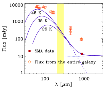
According to the models, the central part of II Zw 40 has a flux of 558, 486, and 347 mJy at 200 $\mu$m (1.5 THz) for $T_{\mathrm{dust}}=45$, 35, and 25 K, respectively. Since the difference is larger at 1.5 THz than at 1.0 THz, it would be better to choose the 1.5 THz window. (Higher THz frequencies would be better just for the purpose of discriminating the dust temperature, but are only available for airborne or space facilities, which are difficult to be equipped with a 10-m class telescope.) According to Hirashita (2013), 61% of the flux is concentrated in the SMA beam, whose size is comparable to the GLT beam at 1.5 THz. Therefore we adopt $347\times 0.61=211$ mJy beam^-1 for the expected GLT flux. With the sensitivity discussed in Section 2.3, it is difficult to detect such an extragalactic star-forming region, although we target the brightest class. However, for continuum, more sensitive bolometer-type facilities may be available. If we could achieve a 10-times better sensitivity (1.9 Jy for 1-sec integration), the above source can be detected with 5 $\sigma$ in an on-source integration time of 30 min. This kind of sensitivity is realistic considering the existing planning such as ArTeMiS. In other words, such a sensitivity as an order of 1 Jy with 1-sec integration is crucial for extragalactic dust studies at THz frequencies.

We list the selected sample in Table 3.3.1. We chose a sample from Klein, Weiland, & Brinks (1991) based on bright radio continuum emission, which is known to correlate with FIR brightness (Hirashita, 2013). We list the BCDs brigher than $1/\sqrt{2}$ of II Zw 40 ($21\pm 2$ mJy) at a wavelength of 2.8 cm, expecting that such galaxies can be detected within the twice of the expected integration time for II Zw 40. This is for one pointing, and a multi-pixel detector is surely required to get a panoramic view of individual galaxies.

Sample of Blue Compact Dwarf Galaxies (BCDs) suitable for GLT observations. Object Other names RA (J2000) Dec (J2000) Distance $12+\log(\mathrm{O/H})$ $S_{\mathrm{2.8~{}cm}}$ Ref. [h m s] [$\arcdeg$ $\arcmin$ $\arcsec$] [Mpc] [mJy] Haro 1 UGC 3930, NGC 2415 07 36 56.7 +35 14 31 52.0 8.40 $21\pm 3$ 1 Mrk 140 10 16 28.2 +45 19 18 22.7 8.30 $18\pm 6$ 2 Mrk 297 NGC 6052, UGC 10182, 16 05 13.0 +20 32 32 63.0 8.65 $22\pm 5$ 3 Arp 209 Mrk 314 NGC 7468, UGC 12329 23 02 59.2 +16 36 19 31.1 8.10 $25\pm 3$ 1 III Zw 102 NGC 7625, UGC 12529, 23 20 30.1 +17 13 32 25.0 8.49 $17\pm 1$ 1 Arp 212 References for $12+\log\mathrm{(O/H)}$: 1) Cairós et al. (2012); 2) Izotov et al. (2006); 3) James et al. (2002).

3.3.2 Metallicity dependence of [N II] 205 $\mu$m line

In Section 3.1.3, we suggested that [N ii] fine-structure line emission is a useful probe of star formation, since it is emitted from H ii regions developed around young massive stars. We also proposed that the comparison with an H$\alpha$ map or radio (free–free emission) map serves as a local calibration of the [N ii] luminosity for a star formation indicator. Here, we propose to extend these studies to an extragalactic sample. In particular, [N ii] 205 $\mu$m emission is poorly focused on even with Herschel, especially because this line is located at the edge of the spectral band (Cormier et al., 2015).

We especially focus on the same BCD sample as above for the purpose of clarifying the metallicity dependence of [N ii] emission as well as confirming that [N ii] emission traces the star formation activities. The correlation between the metallicity and the hardness of stellar radiation field (Hunt et al., 2010) means that both these factors enter the “metallicity dependence” of the intensity of fine-structure lines. To seperate these two factors, observations of other fine-structure lines are necessary (Cormier et al., 2015).

As formulated in Section 3.1.3, it is useful to relate the [N ii] 205 $\mu$m luminosity, $L_{\mathrm{N\,II}}$ to the SFR by introducing the proportionality constant, $C_{\mathrm{N\,II}}$:

$$L_{\mathrm{N\,II}}=C_{\mathrm{N\,II}}\mathrm{SFR}.$$ (12)

Inoue et al. (2014b) derived $C_{\mathrm{NII}}$ as a function of metallicity using the photoionization code cloudy: $\log C_{\mathrm{[N\,II]}}/[\mathrm{(erg~{}s^{-1})/(M_{\odot}~{}yr^{-1})}]=39.82$, 39.07, 37.72, and 36.85 for $Z/\mathrm{Z}_{\odot}=1$, 0.4, 0.2, and 0.02, respectively.

We take an example of II Zw 40 (the same object used in Section 3.3.1) to estimate the detectability of the [N ii] line. For the central $\sim$4 arcsec region of II Zw 40, Beck et al. (2002) derived a flux of 14 mJy at a frequency of 15 GHz. We adopt this frequency, since the free–free emission is probably optically thick at lower frequencies (Hirashita, 2011). Using equation (9) for $\nu=15$ GHz, $T_{e}=10^{4}$ K, and $\Delta\nu=10^{8}$ Hz (corresponding to a velocity width of 20 km s^-1) with the reduced efficiency of [N ii] by 2.1 dex due to the low metallicity (we adopt the value for 0.2 Z_⊙; $C_{\mathrm{H\alpha,N\,II}}=4.14\times 10^{-4}$), we obtain $f_{\mathrm{N\,II}}=58.5(S_{\nu}/\mathrm{mJy})$ Jy. Since the beam size of the GLT is equal to the radio 15 GHz beam above ($\sim 4$ arcsec), the above 15 GHz flux ($S_{\nu}=14$ mJy) indicates that $f_{\mathrm{N\,II}}=6.5$ Jy beam^-1 in the GLT 1.5 THz band. Using the same capability as in Section 2.3, we obtain an rms = 227 Jy beam^-1 at 1.5 THz for a velocity resolution of 10 km s^-1 for a 1-sec integration, an on-source integration time of 3.0 hr is required for a 3 $\sigma$ detection. Since this integration time is realistic, we can test the metallicity dependence of [N ii] 205 $\mu$m luminosity with the same BCD sample as in Section 3.3.1.

Our GLT observations of the [N ii] 205 $\mu$m line in nearby galaxies will provide basic knowledge for the interpretation of high-$z$ [N ii] lines by ALMA. If the metallicity is known for the system, the [N ii] intensity is directly used to determine the SFR of the system. The metallicity can also be estimated by ALMA observation for high-$z$ galaxies, as Nagao et al. (2012) demonstrated that [N ii] 205 $\mu$m/[C ii] 158 $\mu$m flux ratio can be used to estimate the metallicity.

The CO $J=13$–12 line is also in the 1.5 THz window (Table 3.1), but its intensity is much weaker. Therefore, it is not probable that the CO line is also detected in nearby BCDs. Such a highly excited CO line can be emitted from PDRs with extremely high density ($\gtrsim 10^{6.5}$ cm^-3) and extremely high UV intensity ($\sim 10^{5}$ times the interstellar radiation field in the Galaxy) (Meijerink et al., 2007; van der Werf et al., 2010). Indeed, van der Werf et al. (2010) explained the Herschel detection of CO $J=13$–12 in Mrk 231 by X-ray dominated region (XDR). If nearby AGNs have a similar CO $J=13$–12 flux ($\sim 1$ Jy at peak with $\Delta\nu/\nu\sim 8\times 10^{-4}$, corresponding to a velocity width of 240 km s^-1), an on-source integration of $\sim 5.4$ hour is necessary to detect CO $J=13$–12 line with 3 $\sigma$ level in nearby AGNs if we assume the same velocity resolution (240 km s^-1) (see Table 2.3 for the detection limit). Probably, this is too time-consuming for the first-generation ground-based THz telescopes. Because such an extragalactic highly excited region is compact and regarded as a point source, a single-pixel detector will be sufficient for this purpose. The requirement for angular resolution is not severe. Therefore, airborne or space telescopes may be more suitable for the purpose of observing extragalactic highly excited lines.

3.3.3 Possible targets II: the foot points of dust-enriched outflows in starburst galaxies

The metal enrichment of the intergalactic medium (IGM) occurs through the outflow of metals and dust from galaxies (e.g., Adelberger et al., 2003; Kobayashi, Springel, & White, 2007). Outflows from actively star-forming galaxies or starburst galaxies are commonly seen (e.g., Heckman, Armus, & Miley, 1990; Lehnert & Heckman, 1995, 1996). They are often seen in optical emission lines or soft X-ray emission (e.g., Martin, 1998; Dahlem, Weaver, & Heckman, 1998; Strickland et al., 2004; Sharp & Bland-Hawthorn, 2010). Being associated with a starburst activity, outflows are considered to be driven by a large number of supernova explosions. This huge explosion energy blows the surrounding ISM away from the galactic disks mostly in the perpendicular direction to the disks, and creates outflows (e.g., Tomisaka & Ikeuchi, 1988; Strickland & Stevens, 2000). Such a huge energy input to the surrounding ISM affects the activities inside the ISM (i.e., star formation) in the destructive way; namely it terminates the star formation. On the other hand, the expansion of the ISM toward the galactic disk accumulates the ISM and creates new star formation or starburst (Matsushita et al., 2005).

The past observations of outflows have mainly focused on plasma or ionized gas seen in the optical, near-infrared, and X-ray. On the other hand, observations of molecular-gas and dust outflows are very few because of their intrinsic faintness and the limitation of the instruments. Recent improvement of sensitive telescopes and receivers and wide-band backends has started to make images of the molecular gas and dust outflows possible (Figure 11). Recent observations of molecular-gas outflows have revealed that the outflowing mass is dominated by molecular gas, rather than the ionized gas or plasma (Tsai et al., 2009, 2012). This implies that such molecular outflows also contribute to the transport of dust to the IGM and thus to the metal enrichment of the IGM. Imaging of dust outflows is much less explored and is limited mostly to warm/hot dust imaging (e.g., Engelbracht et al., 2006; Kaneda et al., 2009) with cold dust imaging remaining rare (e.g., Alton, Davies, & Bianchi, 1999). Moreover, multi-wavlength information, especially at the dust spectrum peak (around THz) is crucial to derive the mass and temperature of dust.

Recently, because of high sensitivity of Herschel, dust outflows have been observed for some galaxies. In particular, Meléndez et al. (2015) observed a nearby edge-on starburst galaxy, NGC 4631, by Herschel. They found that the structures seen in the dust outflow match extraplanar structures in other outflow tracers such as H$\alpha$ and X-ray. However, because of the low angular resolution of Herschel especially at $\geq 160~{}\micron$, where the dust temperature of “cold” dust component can be correctly determined, the filamentary structures of H$\alpha$ at the foot point of the outflows were not fully traced by the dust. For example, it is difficult to judge if the dust heating is more associated with the shocks in dense molecular gas (outflow) (Beirão et al., 2015) or with the hot plasma. On the other hand, Herschel was suitable for tracing the global structure of the dust outflows. Therefore, a complementary observation focusing on the small-scale foot point structures of dust outflows would be desirable with a high-resolution capability of ground-based THz telescopes.

Figure 11: The Nobeyama Millimeter Array (NMA) CO(1–0) image (contours: Matsushita et al. 2000, 2005) overlaid on the Subaru H$\alpha$ image (color map: Ohyama et al. 2002) for M82. At the distance of M82 (3.9 Mpc; Sakai & Madore, 1999), $1^{\prime\prime}$ corresponds to 19 pc.

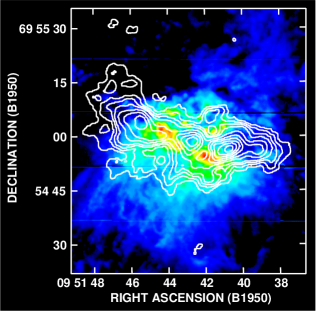
As explained above, the largest advantage of ground-based THz telescopes is high angular resolution. Therefore, we aim at resolving the dust at the foot of outflow. In particular, we focus on relatively dense outflows, that is, molecular outflows shown in Fig. 11. By observing the dust emission in outflows, we will know (1) the dust mass flowing out from galaxies due to the active star formation or starburst activities, (2) the dust temperature and its gradient across the dust outflows, and (3) the relation between dust, molecular gas, and ionized gas, or the dust-to-gas ratio by comparing with the existing images of gas tracers. Using the above information, we will obtain a comprehensive picture of the multi-component outflow.

To the above aim, we first perform THz mapping observations of edge-on actively star-forming galaxies that are already known to have outflows in other wavelengths. For the mapping, we target the interface between molecular outflows and more extended outflows traced with H$\alpha$ or X-ray. As we observe in Figure 11, the interface has structures well below 10 arcsec, which is only traced with the GLT at THz frequencies, i.e., near the SED peak of dust emission. We could also derive the variation of dust tempratures if we observe the object in two THz windows (e.g., 1.0 and 1.5 THz).

Now we estimate the feasilibity of observing the interface between molecular and ionized outflows. Alton et al. (1999) showed the observed dust SED in the outflow of M82 at submm wavelengths. We adopt their pessimistic extrapolation toward shorter wavelengths (i.e., their case with a dust temperature of 13 K), 100 Jy at 200 $\mu$m within a $80^{\prime\prime}\times 36^{\prime\prime}$ region. The flux density within the $4^{\prime\prime}$ beam will therefore be about 0.5 Jy. With the sensitivity adopted in Section 2.3, an on-source integration time of 9 hr is required to detect this signal with 5$\sigma$. However, as mentioned in Section 3.3.1, it may be possible to develop a bolometer-type instrument with an order of magnitude better sensitivity. In this case, we can detect the source with 6 min of on-source integration. Moreover, we used the averaged dust brightness for the above region; in reality, the interface associated with relatively dense molecular outflows probably has an enhanced brightness since the emission flux is concentrated into a small area. Therefore, we may be able to detect the dust associated with the interface within a reasonable time if the sensitive THz bolometer is available. Outflows are extended, so a multi-pixel detector is crucial.

We chose 6 nearby edge-on active star formation and starburst galaxies listed in Table 3.3.3. All these galaxies are known to have H$\alpha$ and X-ray outflows (M82, NGC 2146, and NGC 3628 are known to have molecular outflow). The references are also listed in Table 3.3.3. The total 60 $\mu$m flux $f_{60}$ is also shown for each galaxy. Note that the 60 $\mu$m flux of the galaxies other than M82 is 10–20 times smaller than that of M82; however, we target the interface which may have similar physical conditions (i.e., similar brightness). Therefore, it is worth considering these targets, although we can start observations from M82.

Edge-on sample for outflow studies. Object RA(J2000) Dec(J2000) $d$ $f_{60}\,^{*}$ Ref. [h m s] [$\arcdeg$ $\arcmin$ $\arcsec$] [Mpc] [Jy] M82 09 55 52.7 +69 40 46 3.25 1314 1 NGC 891 02 22 33.4 +42 20 57 9.6 61.1 1 NGC 2146 06 18 37.7 +78 21 25 17.2 131 2 NGC 3079 10 01 57.8 +55 40 47 17.1 50.2 1 NGC 3628 11 20 17.0 +13 35 23 10.0 51.6 1 NGC 4631 12 42 08.0 +32 32 29 7.5 82.9 1 ^∗IRAS 60 $\mu$m flux as an indicator of the entire flux from the galaxy.
References — 1) Strickland et al. (2004); 2) Tsai et al. (2009).

4 Sub-THz science cases

Since satisfactory weather for THz science is realized for a fraction of the total time (Section 2.2), it is worth considering “sub-THz” science cases, which are executed in the non-THz weather conditions. We will put a particular focus on the 350 $\mu$m ($\sim 850$ GHz) and 450 $\mu$m ($\sim$650 GHz) windows, for which the GLT still has an advantage for the good atmospheric condition.

4.1 Bolometer Surveys for High-Redshift Galaxies

It has been known that the received total energy output of the entire universe traced by the so-called extragalactic background light or cosmic background radiation is equally strong in the optical and in the FIR (e.g., Dole et al., 2006). This implies that half of the galaxy and supermassive black hole growth processes are hidden in dust, and that understanding their formation and evolution requires the understanding of their FIR emission. However, the FIR part of the cosmic background has been under-explored, primarily because of the limitation in observational techniques.

Our current understanding of the FIR universe comes from two types of observations: ground-based bolometer-array camera imaging in the mm and submm, and space FIR imaging. The ground-based cameras can resolve approximately 1/3 of the submm background into point sources (e.g., Coppin et al., 2006). Such galaxies are found to be ultraluminous and primarily appear at redshifts between $\sim$1.5 and $\sim$3.5 (e.g., Chapman et al., 2005). The remaining 2/3 of the submm background is unresolved, because of the so-called confusion problem, that is, the low angular resolution of ground-based submm/mm single-dish telescopes. A small sample of them have been studied via strong gravitational lensing (e.g., Chen et al., 2011). The high sensitivity of ALMA has recently resolved most of the mm background into point sources (Hatsukade et al., 2013; Fujimoto et al., 2015). Nevertheless, most of the sources contributing to the peak of the infrared background at sub-THz frequencies ($\lesssim 450~{}\micron$) have yet to be identified. Moreover, as shown below, the galaxy population detected by sub-THz observations is differently biased to the dust temperature and redshift from that traced by submm and mm observations.

Despite the success of ground-based bolometer-array cameras in revealing 1/3 of the submm background population, there is a major drawback. It is widely considered that submm observations only pick up a special population whose dust temperature is relatively low. This strong selection bias is now confirmed by Herschel (e.g., Magnelli et al., 2012). Herschel observations at 70–600 $\mu$m can probe the peak of the infrared dust emission from redshifted galaxies, and are much less biased by dust temperature (see Section 4.1.1). Unfortunately, the small telescope size of Herschel produces an even worse angular resolution than ground-based single-dish telescopes. Only up to 10%–50% (depending on the waveband) of the FIR background was directly resolved by Herschel into individual galaxies (e.g., Berta et al., 2010). The dominant galaxy population that produces the FIR background yet remains to be probed even after Herschel.

4.1.1 Beyond the Confusion Limit of Herschel

Ground-based THz telescopes can make significant breakthrough in this field. Once equipped with a bolometer-array camera in the sub-THz regime, the GLT will have an angular resolution much better than Herschel and existing ground-based submm survey instruments, and thus will have much less confusion problems. For this, the recently commissioned JCMT SCUBA-2 camera (Holland et al., 2013) can serve as an excellent pathfinder. Chen et al. (2013a, b) examined the 450 and 850 $\mu$m number counts obtained with SCUBA-2 in a lensing cluster field. From the comparison with Herschel 350 and 500 $\mu$m results (Oliver et al., 2010), the high angular resolution of the JCMT helps to detect galaxies that are much less luminous (i.e., more normal) than those detected by Herschel. This is true even without the lensing effect. On the other hand, this 450 $\mu$m imaging is still not confusion limited, because of the limited observing time and the site quality.

In the 450 $\mu$m (650 GHz) window, the GLT will have a $9\farcs 5$ resolution (Section 2.3), similar to that of SCUBA-2 at 450 $\mu$m. On the other hand, the GLT will be placed at a site that is much better than Mauna Kea for high-frequency observations (Section 2.2). The SCUBA-2 450 $\mu$m observations by Chen et al. (2013a, b) are still noise limited and far from confusion limited. With the GLT, the site and the substantial observing time will allow confusion limited 350 $\mu$m or 450 $\mu$m imaging. With a 9^′′ resolution at 450 $\mu$m, the confusion limited source density will be approximately 9000 deg^-2, assuming a conservative definition of confusion limit of 30 beams per source. This is close to the limit probed by SCUBA-2 in lensing cluster fields for fully resolving the background.

Figure 12: Dust temperature ($T_{\mathrm{d}}$) vs. total FIR luminosity ($L_{\mathrm{FIR}}$) corresponding to the detection limits assumed for each wavelength (10 mJy, 4 mJy and 3 mJy for 350, 450, and 850 $\mu$m, respectively). Panels (a), (b), and (c) show the results for 350, 450, and 850 $\mu$m, respectively. The solid, dotted, and dashed lines present the relations for galaxies at $z=1$, 2, and 3, respectively. Objects whose total FIR luminosity is larger than (i.e., the right side of) each line are detected. The thick dot-dashed lines show the $T_{\mathrm{d}}$–$L_{\mathrm{FIR}}$ relation derived for a Herschel nearby sample (Symeonidis et al., 2013), for which we apply a linear fit (equation 13). The thin dot-dashed line shows the typical range for the dispersion of dust temperature $\pm$5 K. All the lines are overlaid in Panel (d) with the different thickness: the thick, medium, and thin lines show the results for the 350, 450, and 850 $\micron$, respectively.

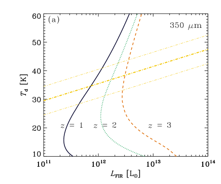
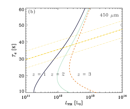
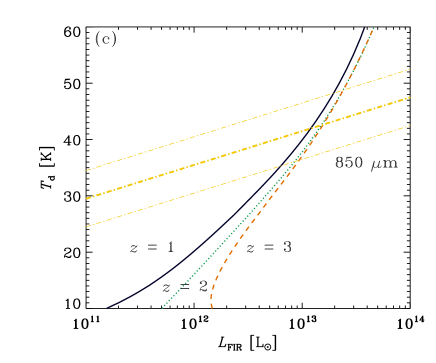
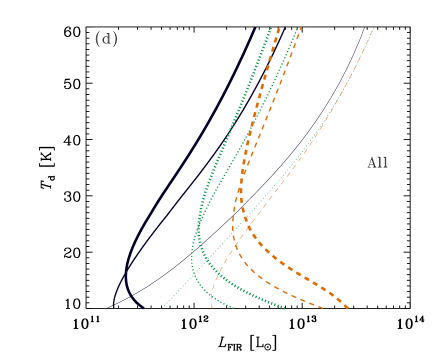
Furthermore, the 450 $\mu$m emission probes galaxies at lower redshifts ($z\sim 1$–2) than those producing the 850 $\mu$m background ($z\sim 2$-4) as demonstrated below. This will allow us to study the majority of star forming galaxies at the peak of the cosmic star formation. As shown below, the bias to cold dust is less at 450 $\mu$m than at 850 $\mu$m. Thus, we can make significant progress in the understanding of galaxy evolution with sub-THz bolometer observations.

To clarify the population expected to be detected by 350 and 450 $\mu$m surveys, we show the relation between the dust temperature, $T_{\mathrm{d}}$, and the total IR luminoisity (total luminosity emitted by dust), $L_{\mathrm{FIR}}$, in Figure 12. We adopt the detection limits of 10, 4, and 3 mJy for 350, 450, and 850 $\mu$m. For 350 and 450 $\mu$m, we adopt the detection limits expected for the above survey design for GLT (aiming at the confusion-limited image; see also Section 4.1.2), while we adopt the 850 $\mu$m detection limit based on Chapman et al. (2005) for a representative 850 $\mu$m survey currently available. We adopt the dust SED model by Totani & Takeuchi (2002), who give the dust SED under given $T_{\mathrm{d}}$ and $L_{\mathrm{FIR}}$. In Figure 12, we plot the minimum $L_{\mathrm{FIR}}$ detected for an object with a dust temperature $T_{\mathrm{d}}$; that is, objects with the FIR luminosity larger than the minimum (or the right side of the curve) can be detected. From Figure 12, we observe that 850 $\mu$m surveys do not have strong redshift dependence, which is due to the so-called negative $K$-correction, and strongly biased against high-$T_{\mathrm{d}}$ objects. This kind of bias was already pointed out by Chapman et al. (2005). In contrast, 350 $\mu$m and 450 $\mu$m surveys are less sensitive to $T_{\mathrm{d}}$, because they trace the emission around the SED peak, which is primarily determined by the total IR luminosity, rather than the dust temperature. On the other hand, the dependence on the redshift is strong at 350 and 450 $\mu$m, because they are out of the wavelength range of strong negative $K$-correction.

For a reference, we also plot in Figure 12 the relation between $T_{\mathrm{d}}$ and $L_{\mathrm{FIR}}$ derived for a Herschel sample at $z\lesssim 1$ by Symeonidis et al. (2013). We applied a linear fit to their relation and obtained

$$T_{\mathrm{d}}=-36.5+6.0\log(L_{\mathrm{FIR}}/L_{\odot}).$$ (13)

The typical dispersion of the dust temprature $\sim$5 K is also shown in the figure. If we assume that this relation is valid for all the redshifts of interest, the FIR luminosity at which equation (13) intersects with each curve in Figure 12 is the minimum detectable FIR luminosity. We observe that the GLT survey at 350–450 $\mu$m can detect galaxies with $L_{\mathrm{FIR}}\gtrsim 10^{12}$ L_⊙ at $z=1$–2. Galaxies with lower dust temperatures are detectable even if the total IR luminosity is a few $\times 10^{11}$ L_⊙. We also observe that the 850 $\mu$m survey only detects extreme galaxies with $L_{\mathrm{FIR}}\gtrsim 10^{13}~{}L_{\odot}$ or fainter galaxies with much lower $T_{\mathrm{d}}$ than expected from the Herschel $T_{\mathrm{d}}$–$L_{\mathrm{FIR}}$ relation.

The FIR luminosities detectable at the sub-THz frequencies, $L_{\mathrm{FIR}}\sim\mbox{a few}\times 10^{11}$–10¹² L_⊙, are typical of galaxies at $z\sim 1$–2 in the sense that such galaxies are located at the knees of luminosity function. In Figure 13, we show the FIR luminosity function derived by Gruppioni et al. (2013) based on Herschel data. We confirm that the depth of the GLT survey at 350 and 450 $\mu$m is suitable to detect the populations down to the knees of luminosity function. Note that the data analysis by Gruppioni et al. (2013) is based on the observational wavelengths $\leq 160~{}\mu$m, so that the uncertainty in the FIR luminosity is large. Our GLT survey will directly catch nearly the peak of the dust SED.

Figure 13: Luminosity function of the total IR luminosity for three redshift ranges, $1.0<z<1.2$, $1.7<z<2.0$, and $2.5<z<3.0$ (solid, dotted, and dashed line, respectively), taken from Gruppioni et al. (2013) (also shown in Burgarella et al. 2013). The vertical dot-dashed line marks a total IR luminosity of $10^{12}$ L_⊙.

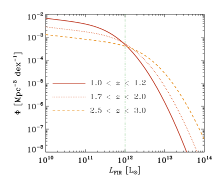
4.1.2 Capability of the GLT and a Possible Survey

Here we discuss the capability of the GLT by comparing it with the JCMT/SCUBA-2. SCUBA-2 has 450 $\mu$m NEFD between 500 and 2000 mJy in a second (Holland et al., 2013). The forecast of NEFD for the bolometer array to be installed in the GLT is 110 mJy, roughly an order of magnitude better than SCUBA-2, making it $\sim 100$ times faster than SCUBA-2 for detecting a point source. To achieve a detection limit of 4 mJy with 3 $\sigma$ at 450 $\mu$m, we require 1.9 hr for the integration time. We assume 3.8 hr for the total on-source observational time per FOV.

The real limiting factor here will be the size of the camera on the GLT. If we assume a camera of $20\times 20$ pixels and Nyquist sampling, the FOV will be 1.65 arcmin². With 1000 hr of observational time, we can survey 430 arcmin², which is comparable to the total area of the famous Great Observatories Origins Deep Survey (GOODS; Giavalisco et al. 2004). It will be unprecedented to cover such an area at the proposed depth at 450 $\mu$m, detecting essentially all important dusty star forming galaxies at $z>0.5$ and nearly fully resolving the background at this waveband.

The most ideal situation is to have a larger camera. If we can increase the number of pixels by a factor of $\sim$10, then we will be capable of covering a significant fraction of a FOV of the Subaru Hyper-Suprime Cam (HSC) (Miyazaki et al., 2012), whose deep imaging will be useful to find the optical counterpart of the GLT-detected sources.

5 Time Variable Sources

We additionally propose science cases for time-variable sources given that some future THz/submm telescopes such as the GLT will allow flexible scheduling of observational time. Long-term monitoring observations are difficult to implement in space THz/submm facilities, which have a limited lifetime, or existing submm interferometers, whose time allocation needs to answer world-wide requests and proposals. In particular, considering monitoring observations at submm (or mm) wavelengths is useful for the purpose of making an efficient use of the time when the weather condition is not suitable for THz observations. In what follows, we explain the importance and uniqueness of this mode of observations, focusing on AGNs.

In another paper, Urata et al. (2015a) discuss a possibility and importance of observing GRB afterglows at submm wavelengths. Since such a ToO type of observational mode is also worth considering, we also give a summary of their paper in Section 5.2.

5.1 Monitoring of AGNs

5.1.1 Exploring VHE $\gamma$-ray flares in Blazars

Constraining the location and emission properties of the very high energy (VHE; $>100$ GeV) $\gamma$-ray emission in AGNs is one of the most important goals of the Fermi mission after 2008 because major extragalactic sources [1017 out of 1319 in the 2nd Fermi-Large Area Telescope (LAT) catalog; $|b|>10^{\circ}$] detected in $\gamma$-rays are AGNs (Ackermann et al., 2011). Among the VHE sources in AGNs, the so-called blazars are identified as the dominant population (97%), including both flat-spectrum radio quasars (FSRQs) and BL Lacertae objects (BL Lacs); they are recognized as the brightest AGN jets pointing very close to our line of sight (Urry & Padovani, 1995).

The $\gamma$-ray emission in blazars at GeV/TeV bands is understood through inverse Compton (IC) scattering of ambient photons. Although various theoretical models have been proposed, the precise location of the $\gamma$-ray emission is poorly constrained. Or perhaps several scenarios at different locations in jets could be considered like in the case of M87 (Abramowski et al., 2012). The IC process takes place either with synchrotron photons from inside the jet via the synchrotron self-Compton (SSC) scattering (e.g., Königl, 1981; Marscher & Gear, 1985), or with external photons (external Compton scattering or EC), where the seed photons are generated in the accretion disk (e.g., Dermer, Schlickeiser, & Mastichiadis, 1992), the circumnuclear material such as the broad-line region (BLR) of quasars (e.g., Sikora, Begelman, & Rees, 1994; Blandford & Levinson, 1995), or the dust torus (e.g., Blażejowski et al., 2000; Böttcher, 2007).

A typical broad-band shape of the SED in blazars exhibits two broad bumps (e.g., Fossati et al., 1998; Ghisellini et al., 1998). The peak of the lower-energy bump between $10^{13}$ and $10^{17}$ Hz is due to the synchrotron emission; moving relativistic shocks in the jet (“shock-in-jet” model) are generally considered for non-thermal particle acceleration (Blandford & Königl, 1979; Marscher, 1980). On the other hand, a high energy bump between $10^{21}$ and $10^{24}$ Hz is due to SSC and/or EC as mentioned above (Abdo et al., 2011), although which of EC and SSC is the dominant mechanism of the high-energy component is not yet conclusive (Ghisellini, Celotti, & Costamante, 2002; Sikora et al., 2009; Zacharias & Schlickeiser, 2012).

In the low-energy component of SED, there is a gap in the frequency coverage between cm/mm and infrared wavelengths. Therefore, single dish observations with the GLT has a capability to fill this gap, contributing to completing the SED. In addition, measurements at these frequencies are important, since the SED peak caused by synchrotron self-absorption is typically located just around these frequencies. Identifying the peak leads to better estimations of the magnetic field strength.

5.1.2 $\gamma$-ray flares at the “far distant” jet downstream

In fact, the VLBI observation including the GLT will play a supplemental role in conducting a unique science program through the GLT single dish monitoring observations toward $\gamma$-ray bright blazars. The goal is to identify the production site of high energy emissions such as X-ray and $\gamma$-ray in blazars, which are referred to as the “blazer zone” and has been believed to be at sub-parsec distances from the nucleus. However, where this energetic site is located is fairly unclear, because a typical size of the VLBI core at mm/cm wavelengths is $\lesssim$ 0.1 mas, corresponding to the de-projected distances $\sim 10$ pc for FSRQs ($\langle z\rangle\sim 1.11$) and $\sim 6$ pc for BL Lacs ($\langle z\rangle\sim 0.37$) at average redshifts (Dermer, 2007) with a viewing angle of 5^∘ for our reference. Thus, if blazar zones are located inside the VLBI core ($\lesssim 10^{5}\,r_{\rm s}$ for $M_{\bullet}=10^{9}M_{\odot}$), it is normally difficult to identify the location of the shock-in-jet to energize particles for synchrotron radiations. Blazer zones, which may be separated from their jet nucleus (possibly far distant downstream $\gg 0.1$–1 pc), have been identified for limited objects in radio galaxies (e.g., Harris et al., 2006; Nagai et al., 2009) and blazars (e.g., Agudo et al., 2011a, b) by direct imaging in mm/cm VLBI observations.

In VLBI observations, we will aim at measuring the sizes and positions of the genuine blazar zone. In order to achieve this, we need to conduct observations with enough angular resolution to resolve 0.01 pc at the blazar distance, and it can only be achieved with submm VLBI observations. Combination of GLT single dish and submm VLBI observations will enable us to achieve that goal very effectively. Here we propose dense monitoring with the single dish observation mode of the GLT to detect a flare event which may indicate activity associated with the blasar zone. If we can detect significant time variation with single dish observations, we can trigger follow-up submm VLBI observations in order to find a new component ejected from the submm VLBI core. Therefore, combined observations between single dish monitoring and sub-mm VLBI imaging play a crucial role in testing the shock-in-jet model.

It was widely believed that the IC process in blazars is dominated within a scale of BLR ($\lesssim 0.1$–1pc) by EC and/or SSC. There is, however, a recent growing recognition that the VHE $\gamma$-ray emitting region may be located at farther distance from the nucleus well beyond the BLR, i.e., over parsecs or even tens of parsecs (e.g., León-Tavares et al., 2011). The VLBA monitoring at 22 and 43 GHz of a sample of Energetic Gamma Ray Experiment Telescope (EGRET) blazars establishes a statistical association of $\gamma$-ray flares with ejections of superluminal components in the parsec-scale regions of the relativistic jet nearby the VLBI radio core (Jorstad et al., 2001). This remarkable finding has been also supported by the single-dish Metsähovi monitoring of total flux density variation at 22 and 37 GHz towards EGRET blazars (Valtaoja & Teräsranta, 1995) with the following conclusion: the highest levels of $\gamma$-ray fluxes are observed during the initial (or peak) stage of radio/mm-wave synchrotron flares.

Among shock-in-jet models, two major possibilities have been discussed; a collision of the faster shock with either the preceding slowly moving shock (“internal shock” model by Spada et al. 2001) or the standing shock complex (Daly & Marscher, 1988; Sokolov, Marscher, & McHardy, Sokolov et al.2004). One of the important clues for positioning VHE $\gamma$-ray flares is the emission size $r_{\gamma}$, which can be roughly constrained by the time variability $t_{\rm var}$ (of the order of day) of flares as

$$r_{\gamma}\lesssim ct_{\rm var}\delta\sim 0.01\left(\frac{t_{\rm var}}{\rm day}\right)\left(\frac{\delta}{10}\right)\ {\rm pc},$$ (14)

where $c$ is the light speed, for a typical case in blazars with a Doppler beaming factor of $\delta\sim\Gamma\sim 10$ ($\theta\sim 1/\Gamma$, where $\Gamma$ is the bulk Lorentz factor $\sim 10$ and $\theta$ is the jet opening angle $\sim$ 0.1 radian). Considering a conical geometry with $\theta\sim 6^{\circ}$, the position of the flare can be placed as $z_{\gamma}\sim r_{\gamma}/\theta\sim 0.1$ pc (along the jet axis $z$), which is comparable to the location of BLR. Therefore, if we consider a case where $z_{\gamma}\gg 0.1$ pc, then the internal shock model in a conical jet may not be appropriated. Instead, non-conical (e.g., parabolic) MHD jet and/or standing shock model as a consequence of the strong over-collimation (jet streamlines are focusing toward the central axis) may be an alternative possibility for a very small region of $r_{\gamma}\lesssim 0.01$ pc at large distance $z_{\gamma}\gg 0.1$ pc.

5.1.3 Lessons learned from the active radio galaxy M87

Why are we interested in the scenario of the far distant jet downstream for $\gamma$-ray flares in AGNs? We have one solid example for VHE TeV $\gamma$-ray event in the nearby active galaxy M87. The flare occurred at a distance $z_{\gamma}\gg 0.1$ pc, but it could be common for AGNs. In what follows, let us introduce our model based on M87 and argue the $\gamma$-ray emission size and its corresponding time variability of the flare in a non-conical jet structure. A supermassive black hole (SMBH) mass of $M_{\bullet}\sim 6.6\times 10^{9}M_{\odot}$ in M87 (Gebhardt et al., 2011), owing to its proximity ($d=16.7$ Mpc, where 1$\arcsec$ corresponds to $\simeq$80 pc; Blakeslee et al. 2009), gives an apparent angular size of $\sim 8\,\mu$as for the Schwarzschild radius $r_{\rm s}\equiv 2GM_{\bullet}/c^{2}$, where $G$ is the gravitational constant, providing a unique opportunity to study the relativistic outflow with the highest angular resolution in units of $r_{\rm s}$ with a moderately large viewing angle of $\theta_{\rm v}\sim 14^{\circ}$ (Wang & Zhou, 2009). Recent extensive studies of the jet toward M87 have revealed a parabolic stream at $\sim 10\,r_{\rm s}$–$10^{5}\,r_{\rm s}$, while it changes into a conical stream beyond $\sim 2\times 10^{6}\,r_{\rm s}$ (Asada & Nakamura, 2012; Nakamura & Asada, 2013), as shown in Fig. 14.

Figure 14: Distribution of the radius of the jet ($r$) as a function of the de-projected distance from the core ($z$) in units of $r_{\rm s}$ (Asada & Nakamura, 2012; Nakamura & Asada, 2013). The solid line is the linear least-square fit for the data points except the three inner points of VLBI cores (at 43, 86, and 230 GHz), indicating the parabolic streamline $z\propto r^{a}$ with $a=1.73\pm 0.05$. On the other hand, the dashed line indicates the conical streamline with $a$ of $0.96\pm 0.1$. The so-called HST-1 complex, a bright feature with sub/super-luminal motions, is located around $5\times 10^{5}\,r_{\rm s}$. The vertical (dashed) line denotes the Bondi accretion radius $R_{\rm B}$, located at $\simeq 3.8\times 10^{5}\,r_{\rm s}$. The horizontal (dotted) line indicates the inner stable circular orbit (ISCO) of the accretion disk for the Schwarzschild black hole.

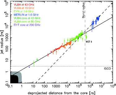
Correspondingly, proper motion analysis suggests that the parabolic part of the jet exhibits bulk acceleration while the conical part shows deceleration. This supports the MHD jet paradigm in M87 (Nakamura & Asada, 2013; Asada et al., 2014). This remarkable finding of the “jet break” (the jet structural transition from a parabolic to conical stream as well as from the acceleration to deceleration of the bulk flow) in M87 indicates a fundamental process of AGN jets interacting with the stratified ISM. The jet break in M87 is presumably associated with the jet over-collimation and thus the formation of a narrower re-confinement nozzle is expected (e.g., Stawarz et al., 2006). Figure 14 also shows that a structured complex known as “HST-1” (Biretta et al., 1999) is located just downstream from the Bondi radius of $R_{\mathrm{B}}\simeq 3.8\times 10^{5}\ r_{\rm s}$ ($\sim 250$ pc in de-projection) (cf. Allen et al., 2006; Cheung et al., 2007, original value of $M_{\bullet}$ is replaced with $\sim 6.6\times 10^{9}M_{\odot}$).

HST-1 consists of bright knots, whose apparent motions are superluminal with a range of $4c$–$6c$, accompanied by subluminal motions (e.g., Biretta et al., 1999; Cheung et al., 2007; Giroletti et al., 2012). The furthest upstream component “HST-1d” in the complex at around $4.4\times 10^{5}\,r_{\rm s}$ ($\sim$ 290 pc in de-projection) seems to be stationary, and has been identified as the origin of sub/superluminal motions as well as the possible site for the TeV $\gamma$-ray flare event in the year 2005 (Cheung et al., 2007). Indeed, the simultaneous rise and fall of light curves at all wavelengths (radio, optical, NUV, and X-ray bands) during 2005 (Aharonian et al., 2006; Harris et al., 2006; Cheung et al., 2007; Madrid, 2009; Abramowski et al., 2012) indicate that the flare was a local event caused by a simple compression at HST-1 (Harris et al., 2006, 2009), which created an increase of the synchrotron energy at all wavelengths equally. The component HST-1c, which had been ejected during 2004–2005 from HST-1d, was presumably associated with the HST-1 flare occurring in 2005 as suggested by Cheung et al. (2007). Recently, Liu et al. (2013) proposed a model for the HST-1 flare in 2005: the brightening/dimming fluxes on multi-wavelength light curves (from radio to X-ray) could be explained as an adiabatic compression/expansion under the conservation of magnetic fluxes when the blob passes through a hourglass or de Laval-nozzle-shaped sheath layer (i.e., the re-confinement magnetic nozzle). In their model, the maximum of the TeV flare in M87 was coincident with the peak of the light curves from radio to X-ray in HST-1 during 2005 (Cheung et al., 2007; Abramowski et al., 2012).

As introduced above in Section 5.1.2, one of the most important clues for positioning VHE flares is the emission size $r_{\gamma}$, which can be roughly constrained by the timescale of $\gamma$-ray flux variability ($t_{\rm var}\sim 2$ days) in M87 around 2005 (Aharonian et al., 2006). This gives $r_{\gamma}\lesssim ct_{\rm var}\delta\sim 0.01\,{\rm pc}\sim 20\,r_{s}$. Based on the assumption that the M87 jet geometry is conical, Aharonian et al. (2006) estimate an unrealistically small opening angle of the jet $\theta\sim 1.5\times 10^{-3}\delta$ degree at $0\farcs 85$ ($\simeq$ 68 pc in projection) along the jet axis for explaining the size of this VHE flare $r_{\gamma}\lesssim 5\delta\,r_{s}$ with disfavoring HST-1 as a possible site of TeV $\gamma$-ray production (i.e., the nucleus of M87). The M87 jet is, however, not conical, but parabolic toward the upstream from HST-1 (Asada & Nakamura, 2012; Nakamura & Asada, 2013). Furthermore, a simultaneous flaring up from radio through optical/X-ray to $\gamma$-ray at HST-1 (Cheung et al., 2007; Harris et al., 2009) strongly suggests that HST-1 could be the most promising site for the TeV $\gamma$-ray emission, while the nucleus exhibited quiescent behaviors at multi-wavelengths (Harris et al., 2009; Madrid, 2009; Abramowski et al., 2012).

Narrowly focused (re-confinement) nozzle in supersonic jets could be produced owing to a lateral imbalance between the jet internal and external ISM pressures (Courant & Friedrichs, 1948); the system consists of a stationary “oblique shocks + a Mach disk”, i.e., a standing shock complex. Physics of the standing shock complex has been been discussed in the extragalactic jet community, starting from the early 1980s (e.g., Sanders, 1983). If we apply this stationary shock system to the HST-1 complex, recurrent events of ejected subluminal blobs from the furthest upstream of the HST-1 complex (Biretta et al., 1999; Cheung et al., 2007; Giroletti et al., 2012) may be due to a lateral compression/expansion of the standing shock complex.

In Figure 14, the maximum radius $r_{\rm max}$ of the parabolic jet can be referred in the vicinity of $R_{\rm B}$. On the other hand, the radial size of the HST-1 complex is about 1/3 of $r_{\rm max}$ although the minimum radius $r_{\rm min}$ of the jet re-confinement nozzle could be much narrower at the maximal focal point (around the Mach disk). Note that the HST-1 complex, which consists of the ejected sub/superluminal blobs, is located in the downstream of the standing feature HST-1d. A magnetic focusing process of MHD jets in a theoretical argument makes a ratio $r_{\rm max}/r_{\rm min}$ by a factor of $\approx 10^{1-2}$ (Achterberg, Blandford, & Goldreich, 1983), while it is restricted to a factor of $\sim 2$ in adiabatic hydrodynamic jets (Sanders, 1983). Giving an upper limit of $r_{\rm max}\simeq 3000\,r_{s}$ (Asada & Nakamura, 2012) (see also Figure 14), a range of $r_{\rm min}\simeq(30-300)\,r_{s}$ would be speculated. In the general framework of MHD jets, $r_{\rm min}$ cannot be smaller than the Alfvén radius (e.g., Pelletier & Pudritz, 1992). Correspondingly, the parabolic jet in M87 exhibits a trans-Aflvénic feature at around $z\sim$ a few of $(100-1000)\,r_{s}$, where the jet radius is about $(30-300)\,r_{s}$ (Nakamura & Asada, 2013). Thus, we also suggest that the HST-1 complex could be the potential site (see also Stawarz et al., 2006; Cheung et al., 2007) of the $\gamma$-ray emission even though a short time variability $t_{\rm var}\sim 2$ day is taken into consideration.

5.1.4 Application of the HST-1 scenario in M87 to blazars

Our recent efforts toward M87 may give a promising clue to the MHD jet paradigm (Nakamura et al., 2010; Asada & Nakamura, 2012; Nakamura & Asada, 2013; Nakamura & Meier, 2014; Asada et al., 2014), while the role of magnetic fields in blazar jets is not well understood. However recent observations have shown some indications of how magnetic fields in blazars are fundamental not only in the jet formation process Zamaninasab et al. (2014), but also in their emission regions on parsec scales Ghisellini et al. (2014). Let us consider that AGN jets (both radio galaxies and blazars) evolve by the MHD process, as is generally believed in theoretical fields. Parabolic streamlines, as a consequence of the lateral balance between the jet internal (magnetic) and external (thermal) pressures (e.g., Zakamska et al., 2008; Komissarov et al., 2009; Lyubarsky, 2009), are suitable for the jet bulk acceleration to the relativistic regime with Lorentz factor $\simeq$ a few tens (e.g., Vlahakis & Königl, 2003; Beskin & Nokhrina, 2006, 2009; Komissarov et al., 2007; Tchekhovskoy et al., 2008). Taking a SMBH mass of $M_{\bullet}=10^{9}M_{\odot}$ as our reference, the Bondi accretion radius can be scaled as

$$R_{\rm B}\simeq\ 30\ {\rm pc}\left(\frac{kT}{{\rm keV}}\right)^{-1}\left(\frac{M_{\bullet}}{10^{9}M_{\odot}}\right),$$ (15)

corresponding to $3.2\times 10^{5}r_{\rm s}$, where $kT\sim 1~{}{\rm keV}$ is adopted as a typical ISM value in X-ray observations.

Assuming the jet structure to be a genuine parabolic shape (e.g., Blandford & Znajek, 1977), which originates at the innermost stable circular orbit (ISCO) of the Schwarzshild black hole $r_{\rm ISCO}=3\,r_{\rm s}$, with $z\propto(r/r_{\rm ISCO})^{2}$, an expanding jet has the maximum radius $r_{\rm max}\simeq 0.16\,{\rm pc}\simeq 1.7\times 10^{3}\,r_{\rm s}$ at $z_{\rm max}\simeq R_{\rm B}$. Again, in a magnetically focusing jet model (Achterberg, Blandford, & Goldreich, 1983), the jet radius is reduced by a factor $f_{\rm cmp}=r_{\rm min}/r_{\rm max}\approx 0.01-0.1$; thus, we could infer $r_{\rm min}\approx 2\times(10^{-3}-10^{-2})$ pc, corresponding to $t_{\rm var}\approx(0.2-2)$ day. Similarly, if we consider that a lateral expansion is faster than the genuine parabolic case (e.g., M87), say, $z\propto(r/r_{\rm ISCO})^{1.6}$ (e.g., Blandford & Payne, 1982), $r_{\rm min}\approx 8\times(10^{-3}-10^{-2})$ pc, corresponding to $t_{\rm var}\approx(0.8-8)$ day, is derived.

Based on the shock-in-jet model (a standing shock complex), which may be triggered at around the Bondi radius $R_{\rm B}\gtrsim 10^{5}\,r_{\rm s}$, we estimate the VHE emission size for AGN jets with $M_{\bullet}=10^{9}M_{\odot}$ as

$$r_{\gamma}\approx(10^{-3}-10^{-1})\ {\rm pc},$$ (16)

with the possible time variability range

$$t_{\rm var}\approx(0.1-10)\ {\rm day}.$$ (17)

Therefore, it may be feasible to consider the distant jet downstream scenario toward parabolic jets in AGNs. It is worth to mention that recent analysis on the minimum variability timescales of Fermi blazars in the GeV band reveal a range $\approx$ (0.01 - 60) day for $M_{\bullet}\simeq(10^{7}$–$10^{10})M_{\odot}$ (Vovk & Neronov, 2013); none of the blazars exhibits variability on a timescale shorter than the black hole horizon light-crossing time and/or the period of rotation around the ISCO.

Why do we need a flux monitoring at submm/mm wavelengths? FSRQ 4C +38.41 (at $z=1.807$) has been very active in GeV bands during last five years. Flux variability in this source from GHz frequencies to GeV energies is examined by Raiteri et al. (2012); there were at least three high states of the GeV emission and multi-flaring peaks are associated with each event. The $\gamma$-ray and optical variability on a one-week timescale were tightly correlated, where the sampling is dense enough. On the other hand, there was also some intrinsic, but weak correlation in light curves between the $\gamma$-ray/optical and mm fluxes (taken by the SMA 1.3 mm band). We suspect that the sampling rate at submm/mm wavelengths is still poor ($>$ a week). In the shock-in-jet scenario, it is generally expected that the flare peak in the submm/mm regime is followed with some time delay by the peak at longer wavelengths (i.e., mm to cm), as a consequence of the jet opacity, as demonstrated in radio light curves (e.g., PKS 1510–089 (FSRQ): Orienti et al., 2013). In conclusion, a dense monitoring mm/sub-mm fluxes toward $\gamma$-ray bright blazars with spanning less than a week is the best strategy in order to test the shock-in-jet model and to explore the site and emission mechanism of the VHE $\gamma$-ray flares in AGNs.

5.1.5 Sample Selection

We started with the original sample of VLBI-detected Fermi sources (Lister et al., 2011). From this sample. we selected 17 sources in Table 5.1.5 with the following criteria:

1. Submm VLBI with the GLT at 345 GHz will have an enough linear resolution to resolve a blazar zone of 0.01 pc. Practically, this condition limits the angular diameter distance to 10³ Mpc ($z<0.37$).

2. Submm VLBI with GLT at 345 GHz will have an enough sensitivity to detect the source without phase-up ALMA. Assuming a flat spectrum of blazar, it requires that the flux $>$ 0.3 Jy.

3. The object is accessible from the GLT site with zenith angle $<60^{\circ}$. It gives the source declination larger than 12^∘.

Measurement of the absolute flux density is expected to be limited by the calibration accuracy, which would be typically 10%. In order to robustly achieve this accuracy, it is desired to achieve thermal noise level three-times better than the calibration error. With this condition, around 4% degradation is expected to contribute to the final accuracy due to the thermal noise. As a result, we need only 30 min for the total on-source time at 345 GHz for all the sources in Table 5.1.5. With taking into account the overhead, it will take one hour for each monitoring. Although the observable sky from Greenland is limited, the same object can be monitored constantly over the winter season. Since time variability on a $\sim$ day–week timescale is expected, we propose to conduct this monitoring every 3–4 days.

Candidate AGNs for monitoring observations with the GLT. Name Alias $z$ Optical ID Flux at 15 GHz [Jy] J0112+2244 S2 0109+22 0.265 BL Lac 0.48 J0319+4130 3C 84 0.0176 Galaxy 19.4 J0721+7120 S5 0716+71 0.31 BL Lac 1.2 J0748+2400 PKS 0745+241 0.4092 QSO 1.15 J0854+2006 OJ 287 0.306 BL Lac 4.67 J0958+6533 S4 0954+65 0.367 BL Lac 1.34 J1104+3812 Mrk 421 0.0308 BL Lac 0.33 J1217+3007 ON 325 0.13 BL Lac 0.36 J1230+1223 M87 0.0044 Galaxy 2.51 J1653+3945 Mrk 501 0.0337 BL Lac 0.87 J1719+1745 OT 129 0.137 BL Lac 0.58 J1806+6949 3C 371 0.051 BL Lac 1.37 J1927+7358 4C +73.18 0.302 QSO 3.71 J2022+6136 OW 637 0.227 Galaxy 2.26 J2143+1743 OX 169 0.2107 QSO 1.09 J2202+4216 BL Lac 0.0686 BL Lac 4.52 J2203+3145 4C +31.63 0.2947 QSO 2.6

5.2 GRBs with the GLT

GRBs are among the most powerful explosions in the Universe and are observationally characterized according to intense short flashes mainly occurring in the high-energy band (prompt emission) and long-lived afterglows seen from the X-ray to radio bands. The discovery of afterglows was a watershed event in demonstrating the following properties of GRBs: a cosmological origin for long-soft and short-hard GRBs (Metzger et al., 1997; Berger et al., 2005; Fox et al., 2005); collimated narrow jets with energy $\sim 10^{51}$ erg for long-soft GRBs (e.g., Frail et al., 2001); association with star forming galaxies (e.g., Djorgovski et al., 1998); and a massive star origin for long-soft GRBs (Hjorth et al., 2003; Stanek et al., 2003). Moreover, GRBs are now being exploited as probes of the high redshift Universe, even at $z\gtrsim 8$ (Tanvir et al., 2009). Because of their extremely high luminosity, the highest-$z$ events at the reionization epoch ($z\sim 8$) have already been observed, and their discovery at $z>10$ is highly possible (e.g., Wanderman & Piran, 2010).

The standard fireball model (e.g., Meszaros & Rees, 1997) predicts a double-shock system: a forward shock (FS) propagating in the external medium, and a reverse shock (RS) propagating into the ejecta. The RS emission uniquely probes the dominant composition (i.e., whether the composition is dominated by baryons or magnetic fields) and properties (such as thickness and Lorentz factor) of the ejecta (e.g., Kobayashi, 2000). These characteristics revealed by the RS can in turn constrain the unknown nature of the central engine and energy extraction mechanism. The brightness and spectral peak of the RS emission depend on the magnetization of ejecta (magnetically-dominated ejecta leads to a weaker RS), and the shock strength (mildly relativistic shock leads to lower peak frequency). It is also thought that the RS generates short-lived intense emission at optical (e.g., Akerlof et al., 1999) and/or radio wavelengths (e.g., Kulkarni et al., 1999; Laskar et al., 2013). Such emission is expected to be 2–3 orders of magnitude brighter than those generated by the FS emission. Hence, for the purpose of probing the high-$z$ Universe with GRBs, it is desirable to detect the emission originating from the RS systematically, whereby we will be able to determine their typical occurrence conditions (Inoue, Omukai, & Ciardi, 2007). Past searches with numerous rapid optical follow-ups failed to detect the RS emission. A possible reason for the missing RS component is that the typical reverse shock synchrotron frequency is far below the optical band. As we demonstrated with a rapid SMA ToO observation of GRB120326A (Urata et al., 2014), mm/submm observations are the key to catching the RS component and understanding the emission mechanism of GRB afterglows.

We identify the following three scientific goals for the GRB studies with the GLT: (i) systematic detection of bright submm emissions originating from RS in the early afterglow phase, (ii) characterization of FS and RS emissions by capturing their peak flux and frequency and performing continuous monitoring, and (iii) detections of GRBs as a result of the explosion of first-generation stars at high redshift through systematic rapid follow-ups. As summarized in Urata et al. (2015a), the light curves and spectra calculated by available theoretical models clearly show that the GLT could play a crucial role in these studies. The main workhorse wavelengths are mm and submm bands, where observations can be managed even under the marginal weather conditions for the THz sciences. Hence, rapid follow-ups will be flexibly managed by the semi-automated responding system for the GRB alerts with secure procedures at the extreme site. We installed the prototype system at the Kiso observatory (Urata et al., 2003). A dedicated GRB satellite, the Space-based Multiband Astronomical Variable Objects Monitor (SVOM; Godet et al., 2012) will be available in the GLT era and the mission will explore the anti-Sun direction for the GRB hunting. The combination of the SVOM and the GLT will be able to make rapid GRB follow-ups without any delay caused by unfavorable visibility and to perform continuous mm/submm monitoring over days. This combination could also address the origin of X-ray flashes (XRFs), which are thought to represent a large portion of the entire GRB population. Three models have been proposed and tested for XRFs: a high redshift origin (Heise, 2003); the off-axis jet model (Yamazaki et al., 2002, 2003; Urata et al., 2015b), which is equivalent to the unification scenario of AGN galaxies; and intrinsic properties (e.g., a subenergetic or inefficient fireball), which may also produce on-axis orphan afterglows (Huang et al., 2002). The third model could be tested by the identification of a delayed RS peak through rapid GLT monitoring.

The flux of the RS component is typically 10–100 mJy at 230 GHz for a GRB at $z=1$ in a day after the burst. Such a flux level is easily detected with the 230 GHz detector planned to be used for the VLBI observation, with an on-source integration time of a few minutes (Section 2.3). For a $z=10$ GRB, we need to detect a flux level of a few mJy; to achieve an rms of 1 mJy, an on-source integration time of 28 min is required based on the median continuum NEFD at 230 GHz in Table 2.3.

6 Possible developments of instruments

Here we summarize possible developments for the future THz and sub-THz observations. As representative cases, we list the efforts for the GLT based on Groppi et al. (2010), Grimes et al. (2014), and Thomas et al. (2015). We refer the interested reader to those papers (in particular, Grimes et al. 2014).

6.1 VLBI Receivers

There are cartridge-type VLBI receivers to cover the 230 GHz and 350 GHz frequency windows. The 230 GHz receiver covers a frequency range from 224 to 238 GHz with a circular polarizer and an IF band of 4–8 GHz. The 350 GHz receiver is a copy of the ALMA band-7 receiver with dual linear polarization and upper/lower side IF bands of 4–8 GHz. The 230 and 350 GHz receivers have been delivered and under integration and testing in the VLBI cryostat.

6.2 350 and 650 GHz Multibeam Receivers

Smithsonian Astrophysical Observatory (SAO) is developing a superconductor-insulator-superconductor (SIS) multibeam array receiver for the 325–375 GHz atmospheric window. A 48-pixel feedhorn array, populated with six eight-pixel modules, will be built with an IF band of 4–6 GHz. The expected receiver noise temperature is 75 K, which is similar to the performance of the SMA receivers. The prototype feedhorn array (provided by Oxford Astrophysics) and the first batch of mixers (provided by Academia Sinica Institute of Astronomy and Astrophysics; ASIAA) are under evaluation. The 650 GHz multibeam array is still in the stage of conceptual studies. A receiver with $\sim$256 pixels is proposed to reach $\sim$4 times the mapping speed of Supercam, a 64-pixel receiver deployed on the 10 m Arizona Radio Observatory Submillimeter Telescope.

6.3 THz Multi-beam Receivers

Small multibeam THz receivers are planned to be built based on the hot-electron-bolometer (HEB) technique. There are two plans for the development: one is a 4-pixel 1.4 THz receiver fed by smooth-wall feedhorns, and the other is a 4-pixel receiver, fed by a Si-lens, at frequency 1.45–1.55 THz. The latter will be extended to 9 pixels in the future. The power limitation of the local oscillator (LO) is the biggest challenge for THz multibeam receivers. SAO is investigating the use of a polarization multiplexing technique with a balanced mixer operation to reduce the power requirement of the HEB array. ASIAA is using a cooled multiplier to increase the total LO power. The expected receiver noise temperature is around 1000–2000 K with an IF band of 0.5–4 GHz.

6.4 Bolometer Arrays

As emphasized in Section 4, it is worth considering bolometer arrays at sub-THz frequencies for large surveys. The NEFD of 40, 110, and 400 mJy beam^-1 with 1-sec integration at 350, 650, and 850 $\micron$, respectively, is feasible with the current technology.

Another effort worth mentioning is the CAMbridge Emission Line Surveyor (CAMELS), which is being developed by SAO and the Detector Physics Group at Cavendish Laboratory. CAMELS is an on-chip spectrometer at frequencies from 103 to 114.7 GHz, providing 512 channels with a spectral resolution of $R=3000$. The CAMELS integrates a 4-probe orthogonal-mode-transducer (OMT), integrated filter band spectrometer (IFBS) and microwave kinetic inductance detectors (MKIDs) on one chip using superconductor technology. The targeted NEPs (noise equivalent power) at the low and the top end of the band are $1\times 10^{-18}~{}\mathrm{W/\sqrt{Hz}}$ and $4\times 10^{-18}~{}\mathrm{W/\sqrt{Hz}}$, respectively. The expected line sensitivities based on our atmospheric conditions are from $5\times 10^{3}~{}\mathrm{mJy~{}km~{}s^{-1}}$ to $3\times 10^{4}~{}\mathrm{mJy~{}km~{}s^{-1}}$.

7 Summary

Our scientific cases described in this paper are broadly categorized into
(A) chemistry and evolution in the diffuse to dense interstellar medium (ISM);
(B) collective or integrated effects of star formation seen in extragalactic objects; and
(C) the time-variable submm Universe.
We review these three categories below. The requirements are briefly summarized in Table 7.

Specific requirements for each scientific objective. Target Frequency $\theta$ ^a $\Delta v\,^{\mathrm{b}}$ Sensitivity^c $t\,^{\mathrm{d}}$ Instrument$\,{}^{\mathrm{e}}$ Section^f Cat.^g ISM CO(13–12) 1.5 THz a few^′′ 0.2 km s^-1 83 Jy beam^-1 30 min Spectrometer 3.1.1 A ISM [N ii] 1.5 THz a few^′′ 2 km s^-1 18 Jy beam^-1 13 min Spectrometer 3.1.3 A ISM continuum 1–1.5 THz a few^′′ — 0.4 Jy beam^-1 34 min THz bolometer 3.2.2 A Polarization 1–1.5 THz a few^′′ — —^h 10 hr Polarimetry 3.2.3 A BCDs (dust) 1.5 THz a few ^′′ — 0.2 Jy beam^-1 30 min THz bolometer 3.3.1 A BCDs ([N ii]) 1.5 THz a few^′′ 10 km s^-1 6.5 Jy beam^-1 3 hr Spectrometer 3.3.2 A Starburst interface 1–1.5 THz a few^′′ — 0.5 Jy beam^-1 6 min THz bolometer 3.3.3 A High-$z$ galaxies 850/650 GHz $\sim$10^′′ — 4 mJy beam^-1 1000 hr Bolometer array 4.1 B AGNs submm — — $\sim$1 Jy beam^-1 30 min VLBI detector 5.1 C GRBs submm — — $\sim$a few mJy 3–48 hr VLBI detector 5.2 C ^aAngular resolution. ^bVelocity (or frequency) resolution, or continuum. ^c1 $\sigma$ noise level requested for detection. ^dIntegration time per pointing. For polarization, the time per source. For the high-$z$ galaxy survey, the total survey time. For AGN monitoring, the total on-source time for all the objects in Table 5.1.5. For GRBs, the total duration of monitoring of a source. ^eSpectrometer or bolometer array. ^fSection discussing the case. ^gCategory in Section 7. ^hSee Section 3.2.3 for the sensitivity estimate.

7.1 Category (A)

For category (A), it is recommended that we explore the new window, that is, terahertz (THz), because of its uniqueness. The scientific importance is summarized in what follows.

The CO $J=13$–12 line at 1.4969 THz is a unique tracer of warm (300–500 K) regions in the vicinity of newly formed stars (Section 3.1.1). An example of detection by APEX (Wiedner et al., 2006) indicates that this observation is feasible with currently available technology. In the diffuse ISM, there are other lines emitted from the species shown in Figure 4. Among them, [N ii] 205 $\mu$m emission is strong enough for the first-generation THz facilities to detect (Section 3.1.3). Observations of [N ii] 205 $\mu$m give a useful “calibration” of fine structure lines as they are often used for star-formation indicators in high-redshift galaxies by ALMA. Using a nearby extragalactic sample with a variety of metallicities, THz spectroscopic observations can test the metallicity dependence of [N ii] 205 $\mu$m emission (Section 3.3.2).

Ground-based THz continuum observations have importance in high angular resolutions. For example, the resolution achieved by the GLT is suitable for resolving the individual star-forming site (Section 3.2.2). THz continuum polarization is also an important scientific target (Section 3.2.3). Since THz is near to the dust spectral energy distribution (SED) peak, we can trace the magnetic field structure of the major dust component responsible for the far-infrared emission. Although it is reasonable to start observations with relatively bright Galactic objects, some possibilities of observing extreme extragalactic star-forming activities are also discussed (Section 3.3). For those objects, the high spatial resolution of the GLT is crucial to extract/resolve the regions of interest. For extragalactic continuum studies, development of sensitive bolometer-type THz detector is desirable.

7.2 Category (B)

For this category, survey-type observations are crucial to obtain a general picture, because only a large number of extragalactic objects can provide a general picture of the star formation activities occuring in the history of the Universe. To utilize the good atmospheric conditions in the GLT site, it is preferable to concentrate on relatively short wavelengths (high frequencies) in the submillimeter (submm) regime. Thus, we target the 350 and 450 $\mu$m ($\sim$850 and $\sim$650 GHz, respectively) windows. The largest advantage of the ground-based THz telescopes is again their high angular resolutions, which are useful to overcome the confusion limit of Herschel (Section 4.1). An area larger than 400 arcmin² can be surveyed with a reasonable observational time ($\sim$1000 hr). Installing the most advanced bolometer arrays is cruicial to maximize the survey efficiency.

7.3 Category (C)

Some ground-based submm–millimeter (mm) telescopes such as the GLT have possibilities of flexible scheduling. This category is unique in the sense that it opens up time-domain submm–mm astronomy. In addition to the target-of-opportunity mode for $\gamma$-ray bursts already discussed in another paper by Urata et al. (2015a), we discussed a possibility of monitoring blasars, which are strongly time-variable (Section 5.1). The collaboration with submm very long baseline interferometry (VLBI) is interesting: if an interesting event is detected in the single-dish observation, a submm VLBI observation mode is triggered. This is a unique science case that connects the VLBI and single dish modes. We should also emphasize that the submm (or THz) emission traces synchrotron emission, which gives constraints on magnetic field strengths. As a consequence, we can address the dynamical properties in which magnetic fields play a central role (e.g., collimation).

7.4 Requirements for instruments

For category (A), because of the diffuse nature of the ISM, a multi-pixel detector is strongly favored. The current status of development of THz detectors was described in Section 6.3. Targetting the 1.5 THz window rather than the 1.0 THz window is better because interesting lines exist (Section 3.1), and the separation from already explored submm wavelengths is larger (Section 3.2).

For category (B), a large submm detector array is required. Multi-band detectors are preferred, considering dust temperature determination. The uniqueness of the GLT site is the good atmospheric condition so that relatively high frequencies referred to as sub-THz ($\sim$850 GHz and $\sim$650 GHz) are preferred to make the maximum use of this uniqueness. These frequencies also have an advantage that they are also covered by Herschel; i.e., the Herschel catalog or survey data can be utilized as input.

For category (C), no particular detector capabilities are required. Thus, for the GLT, we can simply use the mm/submm detectors developed for the VLBI observations. Flexibility of time allocation should be kept if we want to pursue this category.

Appendix A Simulation of Dust Temperature Estimate

We examine how useful adding THz data is to determine the dust temperature. We assume that the dust emission is optically thin, which is valid for the objects of interest in this paper. We adopt a power-law wavelength dependence of the mass absorption coefficient ($\kappa_{\nu}$) of dust at THz frequencies. Then, the flux at frequency $\nu$ is written as

$$f_{\nu}=C\nu^{\beta}B_{\nu}(T),$$ (18)

where $C$ is the normalizing constant, which is proportional to the dust mass multiplied by $\kappa_{\nu}$ [see the footnote for equation (11)], and $B_{\nu}(T)$ is the Planck function. In principle, it is possible to determine both $\beta$ and $T$ if we have data at three or more wavelengths (since $C$ is also unknown). However, as shown by Schnee et al. (2007), errors as small as $\sim 2$% is required to determine both. Thus, we fix $\beta=1.5$ (Hirashita, Hibi, & Shiabi, 2007). Since we focus on the goodness of temperature estimate, the value of $\beta$ chosen does not affect our conclusion. We survey a larger range of $T$ than Schnee et al. (2007), since we target objects with a wide dust temperature range. Our focus is also different from theirs in that we emphasize the importance of THz frequencies; in particular, we include frequencies $>$850 GHz or wavelengths $<$350 $\mu$m into our analysis.

Figure 15: Simulations of dust temperature estimate for maximum error $\Delta=30$%. $T_{\mathrm{real}}$ is the input dust temperature while $T_{\mathrm{fit}}$ is the dust temperature derived by the SED fitting. We use the data at (a) 200, 450, and 850 $\mu$m; (b) 300, 450, and 850 $\mu$m; (c) 450 and 850 $\mu$m, and (d) 200 and 300 $\mu$m.

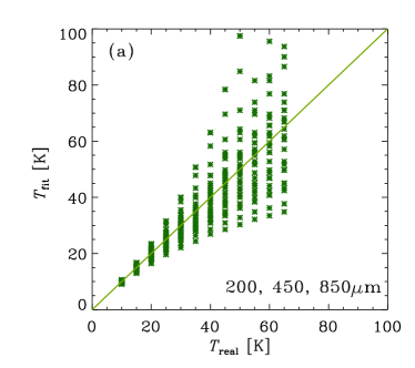
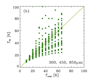
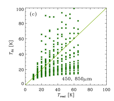
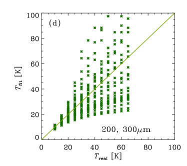
First, we add random noise to the flux calculated by equation (18) and produce “observed fluxes” at a few given wavelengths. Next, based on these artificially made observed fluxes, we estimate the dust temperature. This estimated dust temperature is compared with the input dust temperature to examine how precisely we can obtain the dust temperature. To realize this procedure, we run the following Monte Carlo simulations:

1. With a certain value of $T$, we produce $f_{\nu}$ at given frequencies. Note that the value of $C$ does not affect the temperature estimate so we fix $C$. The given dust temperature is denoted as $T_{\mathrm{real}}$. For the same value of $T_{\mathrm{real}}$, we produce thirty realizations according to the following processes.

2. We add a random independent error to $f_{\nu}$ at each frequency. The percentage of the error $\delta_{f}$ is chosen randomly between $-\Delta$ and $+\Delta$ with $\Delta=30$% chosen unless otherwise stated. The data with the error is denoted as $\tilde{f}_{\nu}=f_{\nu}(1+\delta_{f})$.

3. We fit $\tilde{f}_{\nu}$ at all the wavelengths with equation (18) with two free parameters ($C$ and $T$) by minimizing the sum of the squares of logarithmic difference. The obtained dust temperature is denoted as $T_{\mathrm{fit}}$, which is compared with the input dust temperature, $T_{\mathrm{real}}$.

We examine the following four sets of wavelengths in units of $\mu$m: (200, 450, 850), (300, 450, 850), (450, 850) and (200, 300). The first and second cases are compared to judge which of the THz atmospheric windows, 200 $\mu$m (1.5 THz) or 300 $\mu$m (1.0 THz), in addition to often used submm wavelengths (450 and 850 $\mu$m), is useful to obtain precise dust temperatures. The third case represents the case where we only have submm observations. The last is for the case with only THz observations.

In Figure 15, we show the comparison between the input dust temperature $T_{\mathrm{real}}$ and the obtained dust temperature $T_{\mathrm{fit}}$. Comparing the wavelength sets of (200, 450, 850) and (450, 850) shown in Figures 15a and c, respectively, we find that the addition of 200 $\mu$m improves the dust temperature estimate significantly, especially for the range of dust temperature typical of normal spiral galaxies (15–30 K). This confirms the conclusion drawn by Schnee et al. (2007) that adding a data point at a short wavelength (in their case, 350 $\mu$m) improves the dust temperature estimate. Comparing Figures 15a and b, we find that 200 $\mu$m rather than 300 $\mu$m is preferable to suppress the error at 20–40 K; this is because adding a wavelength farther from the submm wavelengths is more effective. Therefore, the addition of a THz frequency to submm frequencies actually improves the dust temperature estimate and the 1.5 THz (200 $\mu$m) band rather than the 1.0 THz band (300 $\mu$m) is preferable.

The temperature estiamtes with only two THz bands (Figure 15d) is not as good as the combination of a single THz band and submm bands (Figure 15a). This is because the wavelengths of the two THz bands are too close. Therefore, the best scenario is that, in addition to a THz data point, we have multiple submm data with currently available submm interferometers whose angular resolution at submm is comparable to or better than that in the THz bands.

In the above, we assumed conservatively large errors. We expect that, if we increase the number of data points, the temperature estimate becomes more precise. In reality, because of the limited atmospheric window, we cannot increase the number of data points arbitrarily, but rather we can increase the integration time or the band width within technical constraints. This leads to an improvement in the signal-to-noise ratio. Therefore, it is worth examining the effects of signal-to-noise ratio (or error) on the dust temperature estimate.

In Figure 16, we show three cases for various errors $\Delta$: 30% (same as Figure 15c), 10% and 3%. We observe that, if the measurement error is very small, we can get a precise dust temperatures for $T_{\mathrm{dust}}\lesssim 40$ K. Yet, if we add a THz data point with an error $<$10%, the temperature estimate at $T_{\mathrm{dust}}\gtrsim 40$ K is much improved.

Figure 16: Same as Figure 15, but for various errors $\Delta$. Panels (a), (b), and (c) represent the temperature determinations with 450 $\mu$m and 850 $\mu$m data for $\Delta=30$%, 10%, and 3%, respectively. Panel (d) presents the result with an addition of 200 $\mu$m data to Panel (c).

Figure 17: Same as Figure 16, but for the set of wavelengths of (200 $\mu$m, 300 $\mu$m). Panels (a), (b), and (c) represent the temperature determinations with $\Delta=30$% 10%, and 3%, respectively.

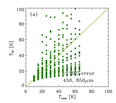
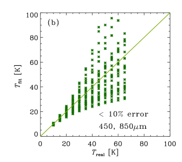
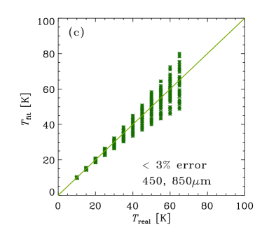
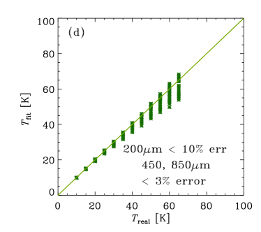
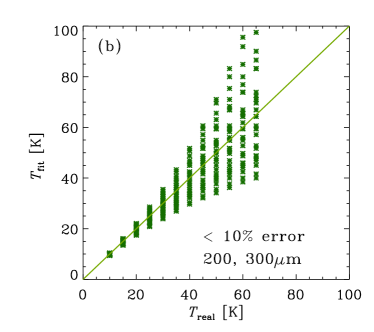
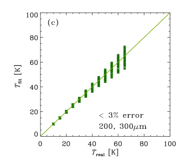
Finally, we also examine the effect of errors on the temperature determination only by the two THz bands in Figure 17. As already shown in Figure 15, if the errors are as large as 30%, we cannot obtain precise values. To obtain a precise enough dust temperature, we need very precise measurements whose typical errors are $\lesssim 3$%. Therefore, we recommend to combine THz observations with submm data obtained by existing submm interferometers.

References

- Abdo et al. (2011) Abdo, A. A., Ackermann, M., Ajello, M., et al. 2011, ApJ, 726, 43
- Abramowski et al. (2012) Abramowski, A., Acero, F., Aharonian, F., et al. 2012, ApJ, 746, 151
- Achterberg, Blandford, & Goldreich (1983) Achterberg, A., Blandord, R. D., & Goldreich, P. 1983, Nature, 304, 607
- Ackermann et al. (2011) Ackermann, M., Ajello, M., Allafort, A., et al. 2011, ApJ, 743, 171
- Adelberger et al. (2003) Adelberger, K. L., Steidel, C. C., Shapley, A. E., & Pettini, M. 2003, ApJ, 584, 45
- Agudo et al. (2011a) Agudo, I, Jorstad, S. G., Marscher, A. P., et al. 2011, ApJ, 726, L13
- Agudo et al. (2011b) Agudo, I. Marscher, A. P., Jorstad, S. G., et al. 2011, ApJ, 735, L10
- Aharonian et al. (2006) Aharonian, F., et al. 2006, Science, 314, 1424
- Akerlof et al. (1999) Akerlof, C., Balsano, R., Barthelmy, S., et al. 1999, Nature, 398, 400
- Allen et al. (2006) Allen, S. W., Dunn, R. J. H., Fabian, A. C., Taylor, G. B., & Reynolds, C. S. 2006, MNRAS, 372, 21
- Alton et al. (1999) Alton, P. B., Davies, J. I., Bianchi, S. 1999, A&A, 343, 51
- Alves, Lombardi, & Lada (2007) Alves, J., Lombardi, M., & Lada, C. J. 2007, ApJ, 462, L17
- Andersson (2012) Andersson, B.-G. 2012, arXiv:1208.4393
- André et al. (2010) André, P., Men’shchikov, A., Bontemps, S., et al. 2010, A&A, 518, L102
- Arzoumanian et al. (2011) Arzoumanian, D., André, P., Didelon, P., et al. 2011, A&A, 529, L6
- Asada & Nakamura (2012) Asada, K., & Nakamura, M. 2012, ApJ, 745, L28
- Asada et al. (2014) Asada, K., Nakamura, M., Doi, A, Nagai, H, & Inoue M, 2014, ApJ, 781, L2
- Beck et al. (2002) Beck, S. C., Turner, J. L., Langland-Shula, L. E., Meier, D. S., Crosthwaite, L. P., & Gorjian, V. 2002, AJ, 124, 2516
- Beirão et al. (2015) Beirão, P., Armus, L., Lehnert, M. D., et al. 2015, MNRAS, 451, 2640
- Berger et al. (2005) Berger, E., Price, P. A., Cenko, S. B., et al. 2005, Nature, 438, 988
- Berta et al. (2010) Berta, S., Magnelli, B., Lutz, D., et al. 2010, A&A, 518, L30
- Beskin & Nokhrina (2006) Beskin, V. S., & Nokhrina, E. E. 2006, MNRAS, 367, 375
- Beskin & Nokhrina (2009) Beskin, V. S., & Nokhrina, E. E. 2009, MNRAS, 397, 1486
- Biretta et al. (1999) Biretta, J. A., Sparks, W. B., & Macchetto, F. 1999, ApJ, 520, 621
- Blain, Barnard, & Chapman (2003) Blain, A. W., Barnard, V. E., & Chapman, S. C. 2003, MNRAS, 338, 733
- Blain et al. (2004) Blain, A. W., Chapman, S. C., Smail, I., & Ivison, R. 2004, ApJ, 611, 52
- Blakeslee et al. (2009) Blakeslee, J. P., Jordán, A., Mei, S., et al. 2009, ApJ, 694, 556
- Blandford & Znajek (1977) Blandford, R., & Znajek, R. L. 1977, MNRAS, 179, 433
- Blandford & Königl (1979) Blandford, R. D., & Königl, A. 1979, ApJ, 232, 34
- Blandford & Payne (1982) Blandford, R. D., & Payne, D. G. 1982, MNRAS, 199, 883
- Blandford & Levinson (1995) Blandford, R. D., & Levinson, A. 1995, ApJ, 441, 79
- Blażejowski et al. (2000) Blażejowski, M., Sikora, M., Moderski, R., & Madejski, G. M. 2000, ApJ, 545, 107
- Böttcher (2007) Böttcher, M., 2007, Ap&SS, 309, 95
- Brauher, Dale, & Helou (2008) Brauher, J. R., Dale, D. A., & Helou, G. 2008, ApJS, 178, 280
- Buat & Xu (1996) Buat, V., & Xu, C. 1996, A&A, 306, 61
- Burgarella et al. (2013) Burgarella, D., et al. 2013, A&A, 554, A70
- Cairós et al. (2012) Cairós, L. M., Caon, N., García Lorenzo, B., Kelz, A., Roth, M., Papaderos, P., & Streicher, O. 2012, A&A, 547, A24
- Caselli et al. (2008) Caselli, P., Vastel, C., Ceccarelli, C., van der Tak, F. F. S., Crapsi, A., & Bacmann, A. 2008, A&A, 492, 703
- Chapman et al. (2005) Chapman, S. C., Blain, A. W., Smail, I., & Ivison, R. J. 2005, ApJ, 622, 772
- Chen et al. (2013a) Chen, C.-C., Cowie, L. L., Barger, A. J., Casey, C. M., Lee, N., Sanders, D. B.; Wang, W.-H., & Williams, J. P. 2013a, ApJ, 762, 81
- Chen et al. (2013b) Chen, C.-C., Cowie, L. L., Barger, A. J., Casey, C. M., Lee, N., Sanders, D. B.; Wang, W.-H., & Williams, J. P. 2013b, ApJ, 776, 131
- Chen et al. (2009) Chen, X., Launhardt, R., & Henning, T. 2009, ApJ, 691, 1729
- Chen et al. (2011) Chen, Y. J., Zhao, G.-Y., & Shen, Z.-Q. 2011, MNRAS, 416, L109
- Cheung et al. (2007) Cheung, C. C., Harris, D. E., & Stawarz, Ł. 2007, ApJ, 663, L65
- Coppin et al. (2006) Coppin, K., et al. 2006, MNRAS, 372, 1621
- Cormier et al. (2015) Cormier, D., et al. 2015, A&A, in press
- Courant & Friedrichs (1948) Courant, R., & Friedriches, K. O. 1948, Supersonic FLow and Shock Waves (New York: Wiley Interscience), p. 387
- Crapsi et al. (2004) Crapsi, A., Caselli, P., Walmsley, C. M., Tafalla, M., Lee, C. W., Bourke, T. L., & Myers, P. C. 2004, A&A, 420, 957
- Cudlip et al. (1982) Cudlip, W., Fruniss, I., King, K. J., & Jennings, R. E. 1982, MNRAS, 200, 1169
- Dahlem, Weaver, & Heckman (1998) Dahlem, M., Weaver, K. A., & Heckman, T. M. 1998, ApJS, 118, 401
- Daly & Marscher (1988) Daly, R. A., & Marscher, A. P. 1988, ApJ, 334, 539
- Deharveng et al. (2001) Deharveng, J.-M., Buat, V., Le Brun, V., Milliard, B., Kunth, D., Shull, J. M., & Gry, C. 2001, A&A, 375, 805
- Dermer, Schlickeiser, & Mastichiadis (1992) Dermer, C. D., Schlickeiser, R., & Mastichiadis, A. 1992, A&A, 256, L27
- Dermer (2007) Dermer, C. D. 2007, ApJ, 659, 958
- Djorgovski et al. (1998) Djorgovski, S. G., Kulkarni, S. R., Bloom, J. S., et al. 1998, ApJ, 508, L17
- Dole et al. (2006) Dole, H., Lagache, G., Puget, J.-L., et al. 2006, A&A, 451, 417
- Dotson et al. (2010) Dotson, J. L., Vaillancourt, J. E., Kirby, L., Dowell, C. D., Hildebrand, R. H., & Davidson, J. A. 2010, ApJS, 186, 406
- Draine (1978) Draine, B. T. 1978, ApJS, 36, 595
- Draine & Anderson (1985) Draine, B. T., & Anderson, N. 1985, ApJ, 292, 494
- Engelbracht et al. (2006) Engelbracht, C. W., Kundurthy, P, Gordon, K. et al. 2006, ApJ, 642, L127
- Engelbracht et al. (2008) Engelbracht, C. W., Rieke, G. H., Gordon, K. D., Smith, J.-D. T., Werner, M. W., Moustakas, J., Willmer, C. N. A., & Vanzi, L. 2008, ApJ, 678, 804
- Enoch et al. (2009) Enoch, M. L., Evans, N. J., II, Sargent, A. I., & Glenn, J. 2009, ApJ, 692, 973
- Espada et al. (2012) Espada, D. et al. 2012, ApJ, 760, L25
- Ferland et al. (2013) Ferland, G. J., Porter, R. L., van Hoof, P. A. M., et al. 2013, RMxAA, 49, 137
- Fossati et al. (1998) Fossati, G., Maraschi, L., Celotti, A., Comastri, A., & Ghisellini, G. 1998, MNRAS, 299, 433
- Fox et al. (2005) Fox, D. B., Frail, D. A., Price, P. A., et al. 2005, Nature, 437, 845
- Foyle et al. (2012) Foyle, K., Wilson, C. D., Mentuch, E., et al. 2012, MNRAS, 421, 2917
- Frail et al. (2001) Frail, D. A., Kulkarni, S. R., Sari, R., et al. 2001, ApJ, 562, L55
- Freedman et al. (1994) Freedman, W. L., Hughes, S. M., Madore, B. F., et al. 1994, ApJ, 427, 628
- Froebrich (2005) Froebrich, D. 2005, ApJS, 156, 169
- Fujimoto et al. (2015) Fujimoto, S., Ouchi, M., Ono, Y., Shibuya, T., Ishigaki, M., Nagai, H., & Momose, R. 2015, ApJ, submitted
- Galliano et al. (2005) Galliano, F., Madden, S. C., Jones, A. P., Wilson, C. D., & Bernard, J.-P. 2005, A&A, 434, 867
- Gebhardt et al. (2011) Gebhardt, K., Adams, J., Richstone, D., et al. 2011, ApJ, 729, 119
- Gerin et al. (2012) Gerin, M., Kazmierczak, M., Jastrzebska, M., et al. 2012, Philosophical Transactions of the Royal Society A: Mathematical, Physical and Engineering Sciences, 370, 5174
- Ghisellini et al. (1998) Ghisellini, G., Celotti, A., Fossati, G., Maraschi, L., & Comastri, A. 1998, MNRAS, 301, 451
- Ghisellini, Celotti, & Costamante (2002) Ghisellini, G., Celotti, A., & Costamante, L. 2002, A&A, 386, 833
- Ghisellini et al. (2014) Ghisellini, G., Tavecchio, F., Maraschi, L., Celotti, A., & Sbarrato, T. 2014, Nature, 515, 376
- Giavalisco et al. (2004) Giavalisco, M., Ferguson, H. C., Koekemoer, A. M., et al. 2004, ApJ, 600, L93
- Girart et al. (2006) Girart, J. M., Rao, R., & Marrone, D. P. 2006, Science, 313, 812
- Girart et al. (2009) Girart, J. M., Beltrán, M. T., Zhang, Q., Rao, R., & Estalella, R. 2009, Science, 324, 1408
- Girart et al. (2013) Girart, J. M., Frau, P., Zhang, Q., et al. 2013, ApJ, 772, 69
- Giroletti et al. (2012) Giroletti, M., Hada, K., Giovannini, G., et al. 2012, A&A, 538, L10
- Godard, Falgarone, & Pineau des Forêts (2008) Godard, B., Falgarone, E., & Pineau des Forêts, G. 2009, A&A, 495, 847
- Godet et al. (2012) Godet, O., Paul, J., Wei, J. Y., et al. 2012, Proc. SPIE, 8443, 84431O
- Goldreich & Kwan (1974) Goldreich, P., & Kwan, J. 1974, ApJ, 189, 441
- Grimes et al. (2014) Grimes, P. K., et al. 2014, Proc. SPIE, 9153, 91531V
- Groppi et al. (2010) Groppi, C., Walker, C., Kulesa, C., et al. 2010, Proc. SPIE, 7741, 77410X
- Gruppioni et al. (2013) Gruppioni, C., Asada, K., Blundell, R., et al. 2013, MNRAS, 432, 23
- Hacar et al. (2013) Hacar, A., Tafalla, M., Kauffmann, J., & Kovács, A. 2013, A&A, 554, A55
- Harris et al. (2006) Harris, D. E., Cheung, C. C., Biretta, J. A., Sparks, W. B., Junor, W., Perlman, E. S., & Wilson, A. S. 2006, ApJ, 640, 211
- Harris et al. (2009) Harri, D. E., Cheung, C. C., Stawarz, Ł., Biretta, J. A., & Perlman, E. S. 2009, ApJ, 699, 305
- Hatchell et al. (2013) Hatchell, J., Wilson, T., Drabek, E., et al. 2013, MNRAS, 429, L10
- Hatsukade et al. (2013) Hatsukade, B., Ohta, K., Seko, A., Yabe, K., & Akiyama, M. 2013, ApJ, 769, L27
- Heckman, Armus, & Miley (1990) Heckman, T. M., Armus, L., & Miley, G. K. 1990, ApJS, 74, 833
- Heise (2003) Heise, J. 2003, in AIP Conf. Proc. 662, Gamma-Ray Burst and Afterglow Astronomy 2001, ed. G. R. Ricker & R. K. Vanderspek (Melville, NY: AIP), 229
- Hildebrand et al. (1984) Hildebrand, R. H., Dragovan, M., & Novak, G. 1984, ApJL, 284, L51
- Hildebrand (1988) Hildebrand, R. H. 1988, QJRAS, 29, 327
- Hildebrand et al. (2000) Hildebrand, R. H., Davidson, J. A., Dotson, J. L., Dowell, C. D., Novak, G., & Vaillancourt, J. E. 2000, PASP, 112, 1215
- Hildebrand et al. (1999) Hildebrand, R.H., Dotson, J.L., Dowell, C.D., Schleuning, D.A., & Vaillancourt, J.E 1999, ApJ, 516, 834
- Hill et al. (2012) Hill, T., André, P., Arzoumanian, D., et al. 2012, A&A, 548, L6
- Hirashita (2011) Hirashita, H. 2011, MNRAS, 418, 828
- Hirashita (2013) Hirashita, H. 2013, MNRAS, 429, 3390
- Hirashita et al. (2003) Hirashita, H., Buat, V., & Inoue, A. K. 2003, A&A, 410, 83
- Hirashita et al. (2007) Hirashita, H., Hibi, Y., & Shibai, H. 2007, MNRAS, 379, 974
- Hirashita & Ichikawa (2009) Hirashita, H., & Ichikawa, T. T. 2009, MNRAS, 396, 500
- Hirashita et al. (2008) Hirashita, H., Kaneda, H., Onaka, T., & Suzuki, T. 2008, PASJ, 60, S477
- Hirota, Ikeda, & Yamamoto (2001) Hirota, T., Ikeda, M., & Yamamoto, S. 2001, ApJ, 547, 814
- Hirotani (2005) Hirotani, K. 2005, ApJ, 619, 73
- Hirota, Ikeda, & Yamamoto (2003) Hirota, T., Ikeda, M., & Yamamoto, S. 2003, ApJ, 594, 859
- Hjorth et al. (2003) Hjorth, J., Sollerman, J., Møller, P., et al. 2003, Nature, 423, 847
- Ho, Moran, & Lo (2004) Ho, P. T. P., Moran, J. M., & Lo, K. Y. 2004, ApJ, 616, L1
- Holland et al. (2013) Holland, W. S., Bintley, D., Chapin, E. L., et al. 2013, MNRAS, 430, 2513
- Huang et al. (2002) Huang, Y. F., Dai, Z. G., & Lu, T. 2002, MNRAS, 332, 735
- Huchtmeier & Day (1975) Huchtmeier, W. K., & Day, G. A. 1975, A&A, 41, 153
- Hull et al. (2014) Hull, C. L. H., Plambeck, R. L., Kwon, W., et al., 2014, ApJS, 213, 13
- Hunt, Bianchi, & Maiolino (2005) Hunt, L. K., Bianchi, S., & Maiolino, R. 2005, A&A, 434, 849
- Hunt et al. (2010) Hunt, L. K., Thuan, T. X., Izotov, Y. I., & Sauvage, M. 2010, ApJ, 712, 164
- Inoue, Hirashita, & Kamaya (2000) Inoue, A. K., Hirashita, H., & Kamaya, H. 2000, PASJ, 52, 539
- Inoue et al. (2014b) Inoue, A. K., Shimizu, I., Tamura, Y., Matsuo, H., Okamoto, T., & Yoshida, N. 2014, ApJ, 780, L18
- Inoue et al. (2014a) Inoue, M., Algaba-Marcos, J. C., Asada, K., et al. 2014, Radio Science, 49, 564
- Inoue et al. (2007) Inoue, S., Omukai, K., & Ciardi, B. 2007, MNRAS, 380, 1715
- Izotov et al. (2006) Izotov, Y. I., Stasińska, G., Meynet, G., Guseva, N. G., & Thuan, T. X. 2006, A&A, 448, 955
- James et al. (2002) James, A., Dunne, L., Eales, S., & Edmunds, M. G. 2002, MNRAS, 335, 753
- Johnstone & Bally (1999) Johnstone, D., & Bally, J. 1999, ApJ, 510, L49
- Jørgensen et al. (2007) Jørgensen, J. K., Bourke, T. L., Myers, P. C., et al. 2007, ApJ, 659, 479
- Jorstad et al. (2001) Jorstad, S. G., Marscher, A. P., Mattox, J. R., Wehrle, A. E., Bloom, S. D., & Yurchenko, A. V. 2001, ApJS, 134, 181
- Jorstad et al. (2010) Jorstad, S. G., Marscher, A. P., Larionov, V. M., et al. 2010, ApJ, 715, 362
- Kaneda et al. (2010) Kaneda, H., et al. 2010, A&A, 514, A14
- Kaneda et al. (2009) Kaneda, H., Yamagishi, M., Suzuki, T., & Onaka, T. 2009, ApJ, 698, L125
- Kawamura et al. (2002) Kawamura, J., Hunter, T. R., Tong, C.-Y., et al. 2002, A&A, 394, 271
- Kennicutt (1998) Kennicutt, R. C., Jr. 1998, ARA&A, 36, 189
- Kennicutt et al. (2007) Kennicutt, R. C., Jr., Calzetti, D., Walter, F., et al. 2007, ApJ, 671, 333
- Klein, Weiland, & Brinks (1991) Klein, U., Weiland, H., & Brinks, E. 1991, A&A, 246, 323
- Kobayashi, Springel, & White (2007) Kobayashi, C., Springel, V., & White, S. D. M. 2007, MNRAS, 376, 1465
- Kobayashi (2000) Kobayashi, S. 2000, ApJ, 545, 807
- Koch et al. (2012) Koch, P. M., Tang, Y.-W., & Ho, P. T. P. 2012, ApJ, 747, 79
- Koch et al. (2013) Koch, P. M., Tang, Y.-W., & Ho, P. T. P. 2013, ApJ, 775, 77
- Koch et al. (2014) Koch, P. M., Tang, Y.-W., & Ho, P. T. P., et al. 2014, ApJ, 797, 99
- Königl (1981) Königl, A. 1981, ApJ, 243, 700
- Könyves et al. (2010) Könyves, V., André, P., Men’shchikov, A., et al. 2010, A&A, 518, L106
- Komissarov et al. (2007) Komissarov S. S., Barkov, M. V., Vlahakis, N., & Königl, A. 2007, MNRAS, 380, 51
- Komissarov et al. (2009) Komissarov, S. S., Vlahakis, N., Königl, A.,Barkov, M. V. 2009, MNRAS, 394, 1182
- Kulkarni et al. (1999) Kulkarni, S. R., Frail, D. A., Sari, R., et al. 1999, ApJ, 522, L97
- Lai et al. (2001) Lai, S.-P., Crutcher, R. M., Girart, J. M. & Rao, R. 2001, ApJ, 561, 864
- Lai et al. (2003) Lai, S.-P., Girart, J. M., & Crutcher, R. M. 2003, ApJ, 598, 392
- Laskar et al. (2013) Laskar, T., Berger, E., Zauderer, B. A., et al. 2013, ApJ, 776, 119
- Lazarian (2007) Lazarian, A. 2007, Journal of Quantitative Spectroscopy and Radiative Transfer, 106, 225
- Lazarian & Hoang (2007) Lazarian, A., & Hoang, T. 2007, MNRAS, 378, 910
- Lehnert & Heckman (1995) Lehnert, M. D., & Heckman, T. M. 1995, ApJS, 97, 89
- Lehnert & Heckman (1996) Lehnert, M. D., & Heckman, T. M. 1996, ApJ, 462, 651
- León-Tavares et al. (2011) León-Tavares, J., Valtaoja, E., Tornikoski, M., Lähteenmäki, A., & Nieppola, E. 2011, A&A, 532, A146
- Leung, Herbst, & Huebner (1984) Leung, C. M., Herbst, E., & Huebner, W. F. 1984, ApJS, 56, 231
- Lisenfeld & Ferrara (1998) Lisenfeld, U., & Ferrara, A. 1998, ApJ, 496, 145
- Lister et al. (2011) Lister, M., Aller, M., Aller, H., et al. 2011, ApJ, 742, 27
- Liu et al. (2010) Liu, Y., Jiang, D. R., Shen, Z.-Q., & Karousos, M. 2010, A&A, 522, A5
- Liu et al. (2011) Liu, H. T., Bai, J. M., & Wang, J. M. 2011, MNRAS, 414, 155
- Liu et al. (2012) Liu, H. B., Quitana-Lacaci, G., Wang, K., Ho, P. T. P., Li, Z.-Y., Zhang, Q., & Zhang, Z.-Y. 2012, ApJ, 745, 61
- Liu et al. (2013) Liu, W.-P., Zhao, G.-Y., Chen, Y. J., Wang, C.-C., Shen, Z.-Q. 2013, ApJ, 146, 15
- López-Sepulcre et al. (2013) López-Sepulcre, A., Taquet, V., Sánchez-Monge, Á., et al. 2013, A&A, 556, A62
- Lobanov (1998) Lobanov, A. P. 1998, A&A, 330, 79
- Lyubarsky (2009) Lyubarsky, Y. 2010, ApJ, 698, 1570
- Madden et al. (2013) Madden, S. C., Rémy-Ruyer, A., Galametz, M., et al. 2013, PASP, 125, 600
- Madrid (2009) Madrid, J. P. 2009, ApJ, 137, 3864
- Magnelli et al. (2012) Magnelli, B., Lutz, D., Santini, P., et al. 2012, A&A, 539, 155
- Mangum et al. (2006) Mangum, J. G., Baars, J. W. M., Greve, A., Lucas, R., Snel, R. C., Wallace, P., & Holdaway, M., 2006, PASP, 118, 1257
- Marrone et al. (2004) Marrone, D. P., Battat, J., Bensch, F., et al. 2004, ApJ, 612, 940
- Marscher (1980) Marscher, A. P. 1980, ApJ, 235, 386
- Marscher & Gear (1985) Marscher, A. P., & Gear, W. K., 1985, ApJ, 298, 114
- Marscher et al. (2010) Marscher, A. P., Jorstad, S. G., Larionov, V. M., et al. 2010, ApJ, 710, L126
- Martin (1998) Martin, C. L. 1998, ApJ, 506, 222
- Martin-Cocher et al. (2014) Martin-Cocher, P. L., Asada, K., Matsushita, S., Chen, M.-T., Ho, P. T. P., Chen, C.-P. 2014, SPIE, 9147, 91473N
- Masunaga & Inutsuka (2000) Masunaga, H., & Inutsuka, S. 2000, ApJ, 531, 350
- Mathis (2000) Mathis, J. S. 2000, in Allen’s Astrophysical Quantities, 4th edition, ed. A. N. Cox (New York: Springer), 523
- Matsushita (2011) Matsushita, S. 2011, in Astronomical Site Testing Data in Chile, ed. M. Curé, et al. Revista Mexicana de Astronomía y Astrofísica (Serie de Conferencias), 41, 95
- Matsushita et al. (1999) Matsushita, S., Matsuo, H., Pardo, J. R., & Radford, S. J. E. 1999, PASJ, 51, 603
- Matsushita & Matsuo (2003) Matsushita, S., & Matsuo, H. 2003, PASJ, 55, 325
- Matsushita et al. (2000) Matsushita, S., Kawabe, R., Matsumoto, H., Tsuru, T. G., Kohno, K., Morita, K.-I., Okumura, S. K., & Vila-Vilaro, B., 2000, ApJ, 545, L107
- Matsushita et al. (2005) Matsushita, S., Kawabe, R., Kohno, K., Matsumoto, H., Tsuru, T.G., & Vila-Vilaro, B. 2005, ApJ, 618, 712
- Matthews et al. (2009) Matthews, B. C., McPhee, C. A., Fissel, L. M., & Curran, R. L. 2009, ApJS, 182, 143
- McKee & Ostriker (2009) McKee C. F., & Ostriker E. C. 2007, ARA&A, 45, 565
- McKee & Ostriker (1977) McKee, C. F., & Ostriker, J. P. 1977, ApJ, 218, 148
- McKinney (2006) McKinney, J. C. 2006, MNRAS, 368, 1561
- Meléndez et al. (2015) Meléndez, M., Veilleux, S., Martin, C., et al. 2015, ApJ, 804, 46
- Meijerink et al. (2007) Meijerink, R., Spaans, M., & Israel, F. P. 2007, A&A, 461, 793
- Menten et al. (2007) Menten, K. M., Reid, M. J., Forbrich, J., & Brunthaler, A. 2007, A&A, 474, 515
- Meszaros & Rees (1997) Meszaros, P., & Rees, M. J. 1997, ApJ, 476, 232
- Metzger et al. (1997) Metzger, M. R., Djorgovski, S. G., Kulkarni, S. R., et al. 1997, Nature, 387, 878
- Mezger, Smith, & Churchwell (1974) Mezger, P. G., Smith, L. F., & Churchwell, E. 1974, A&A, 32, 269
- Miyazaki et al. (2012) Miyazaki, S., Komiyama, Y., Nakaya, H., et al. 2012, SPIE, 8446, 84460Z
- Morata & Herbst (2008) Morata, O., & Herbst, E. 2008, MNRAS, 390, 1549
- Murakami et al. (2007) Murakami, H., Baba, H., Barthel, P., et al. 2007, PASJ, 59, S369
- Myers (2009) Myers, P. C. 2009, ApJ, 700, 1609
- Nagai et al. (2009) Nagai, H., Asada, K., Doi, A., Kameno, S., & Inoue, M. 2009, AN, 330, 161
- Nagao et al. (2012) Nagao, T., Maiolino, R., De Breuck, C., Caselli, P., Hatsukade, B., & Saigo, K. 2012, A&A, 542, L34
- Najita, Ádámkovics, & Glassgold (2011) Najita, J. R., Ádámkovics, M., & Glassgold, A. E. 2011, ApJ, 743, 147
- Nakamura et al. (2010) Nakamura, M., Garofalo, D. & Meier, D. L. 2010, ApJ, 721, 1783
- Nakamura & Asada (2013) Nakamura, M., & Asada, K. 2013, ApJ, 775, 118
- Nakamura & Meier (2014) Nakamura, M. & Meier, D. L. 2014, ApJ, 785, 152
- Narayan et al. (2003) Narayan, R., Igumenshchev, I. V., & Abramowicz, M. A. 2003, PASJ, 55, L69
- Oberst et al. (2006) Oberst, T. E., Parshley, S. C.; Stacey, G. J., et al. 2006, ApJ, 652, L125
- Oberst et al. (2011) Oberst, T. E., Parshley, S. C., Nikola, T., Stacey, G. J., Löhr, A., Lane, A. P., Stark, A. A., & Kamenetzky, J. 2011, ApJ, 739, 100
- Ohyama et al. (2002) Ohyama, Y., Taniguchi, Y., Iye, M., et al. 2002, PASJ, 54, 891
- Oliver et al. (2010) Oliver, S. J., Wang, L., Smith, A. J., et al. 2010, A&A, 518, L21
- Orienti et al. (2013) Orienti, M., Koyama, S., D’Ammando, F. et al. 2013, MNRAS, 428, 2418
- Osterbrock & Ferland (2006) Osterbrock, D. E., & Ferland, G. J. 2006, Astrophysics of Gaseous Nebulae and Active Galactic Nuclei, 2nd ed. (Sausalito, CA: University Science Books)
-
Paine (2012)
Paine, S. 2012 SMA Tech. Memo. version 7.2, 152,
http://www.cfa.harvard.edu/sma/memos/152.pdf - Paine et al. (2000) Paine, S., Blundell, R., Papa, D. C., Barrett, J. W., & Radford, S. J. E. 2000, PASP, 112, 108
- Pelletier & Pudritz (1992) Pelletier, G., & Pudritz, R. E. 1992, ApJ, 394, 117
- Pérez-Beaupuits et al. (2012) Pérez-Beaupuits, J. P., Wiesemeyer, H., Ossenkopf, V., Stutzki, J., Güsten, R., Simon, R., Hübers, H.-W., & Ricken, O. 2012, A&A, 542, L13
- Perlman et al. (2003) Perlman, E. S., Harris, D. E., Biretta, J. A., Sparks, W. B., & Macchetto, F. D. 2003, ApJ, 599, L65
- Perlman et al. (2011) Perlman, E. S., Adams, S. C., Cara, M., et al. 2011, ApJ, 743, 119
- Peterson et al. (2003) Peterson, J. B., Radford, S. J. E., Ade, P. A. R., Chamberlin, R. A., O’Kelly, M. J., Peterson, K. M., & Schartman, E. 2003, PASP, 115, 383
- Pilbratt et al. (2010) Pilbratt, G. L., Riedinger, J. R., Passvogel, T., et al. 2010, A&A, 518, L1
- Pillai et al. (2011) Pillai, T., Kauffmann, J., Wyrowski, F., Hatchell, J., Gibb, A. G., & Thompson, M. A. 2011, A&A, 530, A118
- Pineda et al. (2010) Pineda, J. E., Goodman, A. A., Arce, H. G., et al. 2010, ApJ, 712, L116
- Pohlen et al. (2010) Pohlen, M., Cortese, L., Smith, M. W., et al. 2010, A&A, 518, L72
- Pu et al. (2015) Pu, H.-Y., Nakamura, M., Hirotani, K., Mizuno Y, Wu, K.-W., & Asada, K. 2015, ApJ, 801, 56
- Qiu et al. (2013) Qiu, K., Zhang, Q., Menten, K. M., Liu, H.-Y. B., & Tang, Y.-W. 2013, ApJ, 779, 182
- Raiteri et al. (2012) Raiteri, C. M., et al. 2012, A&A, 545, A48
- Rao et al. (2009) Rao, R., Girart, J. M., Marrone, D. P., Lai, S.-P., & Schnee, S. 2009, ApJ, 707, 921
- Rémy-Ruyer et al. (2014) Rémy-Ruyer, A., Madden, S. C., Galliano, F., et al. 2014, A&A, 557, A95
- Revéret et al. (2014) Revéret, V., André, P., Le Pennec, J., et al. 2014, Proc. SPIE, 9153, 915305
- Rolffs et al. (2010) Rolffs, R., Schilke, P., Comito, C., et al. 2010, A&A, 521, L46
- Rumble et al. (2015) Rumble, D., Hatchell, J., Gutermuth, R. A., et al. 2015, MNRAS, 448, 1551
- Sakai & Madore (1999) Sakai, S., & Madore, B. F. 1999, ApJ, 526, 599
- Salji et al. (2015) Salji, C. J., Richer, J. S., Buckle, J. V., et al. 2015, MNRAS, 449, 1782
- Sanders (1983) Sanders, R. H. 1983, ApJ, 266, 73
- Schmidt & Boller (1993) Schmidt, K.-H., & Boller, T. 1993, AN, 314, 361
- Schinzel et al. (2012) Schinzel, F. K., Lobanov, A. P., Taylor, G. B., Jorstad, S. G., Marscher, A. P., & Zensus, J. A. 2012, A&A, 537, A70
- Schnee et al. (2007) Schnee, S., Kauffmann, J., Goodman, A., & Bertoldi, F. 2007, ApJ, 657, 838
- Schneider & Elmegreen (1979) Schneider, S., & Elmegreen, B. G. 1979, ApJS, 41, 87
- Schöier et al. (2005) Schöier, F. L., van der Tak, F. F. S., van Dishoeck, E. F., & Black, J. H. 2005, A&A, 432, 369
- Scoville & Solomon (1974) Scoville, N. Z., & Solomon, P. M. 1974, ApJ, 187, L67
- Sharp & Bland-Hawthorn (2010) Sharp, R. G., & Bland-Hawthorn, J. 2010, ApJ, 711, 818
- Shiino et al. (2013) Shiino, T., Furuya, R., Soma, T., et al. 2013, in New Trends in Radio Astronomy in the ALMA Era, ed. R. Kawabe, N. Kuno, & S. Yamamoto, ASP Conf. Ser., 476 (ASP: San Francisco), 419
- Shimajiri et al. (2008) Shimajiri, Y., Takahashi, S., Takakuwa, S., Saito, M., & Kawabe, R. 2008, ApJ, 683, 255
- Shirley et al. (2000) Shirley, Y. L., Evans, N. J., II, Rawlings, J. M. C., & Gregersen, E. M. 2000, ApJS, 131, 249
- Sikora, Begelman, & Rees (1994) Sikora, M., Begelman, M. C., & Rees, M. J. 1994, ApJ, 421, 153
- Sikora et al. (2009) Sikora, M., Stawarz, L., Moderski, R., Nalewajko, K., & Madejski, G. M. 2009, ApJ, 704, 38
- (240) Sokolov, A., Marscher, A. P., & McHardy, I. M. 2004, ApJ, 613, 725
- Spada et al. (2001) Spada, M., Ghisellini, G. Lazzati, D., & Celotti, A. 2001, MNRAS, 325, 1559
- Stanek et al. (2003) Stanek, K. Z., Matheson, T., Garnavich, P. M., et al. 2003, ApJ, 591, L17
- Stawarz et al. (2006) Stawarz, Ł., Aharonian, F., Kataoka, J., Ostrowski, M., Siemiginowska, A., & Sikora, M. 2006, MNRAS, 370, 981
- Strickland et al. (2004) Strickland, D. K., Heckman, T. M., Colbert, E. J. M., Hoopes, C. G., & Weaver, K. A. 2004, ApJS, 151, 193
- Strickland & Stevens (2000) Strickland, D. K., & Stevens, I. R. 2000, MNRAS, 314, 511
- Sun & Hirashita (2011) Sun, A.-L., & Hirashita, H. 2011, MNRAS, 411, 1707
- Suzuki et al. (1992) Suzuki, H., Yamamoto, S., Ohishi, M., Kaifu, N., Ishikawa, S., Hirahara, Y., & Takano, S. 1992, ApJ, 392, 551
- Symeonidis et al. (2013) Symeonidis, M., Vaccari, M., Berta, S., et al. 2013, MNRAS, 431, 2317
- Takahashi et al. (2013) Takahashi, S., Ho., P. T. P., Teixeira, P. S., Zapata, L. A., & Su, Y.-N. 2013, ApJ, 763, 57
- Takahashi et al. (2012) Takahashi, S., Saigo, K., Ho, P. T. P., & Tomida, K. 2012, ApJ, 752, 10
- Takakuwa et al. (2004) Takakuwa, S., Saito, M., Lim, J., et al. 2004, ApJ, 616, L15
- Takakuwa & Kamazaki (2011) Takakuwa, S., & Kamazaki, T. 2011, PASJ, 63, 921
- Takakuwa et al. (2012) Takakuwa, S., Saito, M., Lim, J., Saigo, K., Sridharan, T. K., & Patel, N. A. 2012, ApJ, 754, 52
- Tang et al. (2013) Tang, Y.-W., Ho, P. T. P., Koch, P. M., Guilloteau, S., & Dutrey, A. 2013, ApJ, 763, 135
- Tang et al. (2009) Tang, Y.-W., Ho, P. T. P., Koch, P. M., Girart, J. M., Lai, S.-P., & Rao, R. 2009, ApJ, 700, 251
- Tang et al. (2010) Tang, Y.-W., Ho, P. T. P., Koch, P. M., & Rao, R. 2010, ApJ, 717, 1262
- Tanvir et al. (2009) Tanvir, N. R., Fox, D. B., Levan, A. J., et al. 2009, Nature, 461, 1254
- Tavecchio et al. (2011) Tavecchio, F., Becerra-Gonzalez, B.-G., Ghisellini, G., Stamerra, A., Bonnoli, G., Bonnoli, G., Foschini, F., & Maraschi, L. 2011, A&A, 534, A86
- Tchekhovskoy et al. (2008) Tchekhovskoy, A., McKinney, J. C., & Narayan, R. 2008, MNRAS, 388, 551
- Tchekhovskoy et al. (2011) Tchekhovskoy, A., Narayan, R., & McKinney, C. 2011, MNRAS, 418, L79
- Teixeira et al. (2015) Teixeira, P. S., et al. 2015, A&A, submitted
- Thomas et al. (2015) Thomas, C. N., Withington, S., Maiolino, R., et al. 2015, in the proceedings of the 24th International Symposium on Space Terahertz Technology (ISSTT), submitted (arXiv:1401.4395)
- Tomisaka & Ikeuchi (1988) Tomisaka, K., & Ikeuchi, S. 1988, ApJ, 330, 695
- Totani & Takeuchi (2002) Totani, T., & Takeuchi, T. T. 2002, ApJ, 570, 470
- Tremblin et al. (2011) Tremblin, P., Minier, V., Schneider, N., et al. 2011, A&A, 535, A112
- Tremblin et al. (2012) Tremblin, P., Schneider, N., Minier, V., Durand, G. Al., Urban, J. 2012, A&A, 548, A65
- Tsai et al. (2012) Tsai, A.-L., Matsushita, S., Kong, A. K. H., Matsumoto, H., & Kohno, K. 2012, ApJ, 752, 38
- Tsai et al. (2009) Tsai, A.-L., Matsushita, S., Nakanishi, K., et al. 2009, PASJ, 61, 237
- Turner & Beck (2004) Turner, J. L., & Beck, S. C. 2004, ApJ, 602, L85
- Urata et al. (2015a) Urata, Y., Huang, K., Asada, K., et al. 2015a, Advances in Astronomy, Volume 2015 (2015), Article ID 165030
- Urata et al. (2014) Urata, Y., Huang, K., Takahashi, S., et al. 2014, ApJ, 789, 146
- Urata et al. (2015b) Urata, Y., Huang, K., Yamazaki, R., & Sakamoto, T. 2015b, ApJ, 806, 222
- Urata et al. (2003) Urata, Y., Nishiura, S., Miyata, T., et al. 2003, ApJ, 595, L21
- Urry & Padovani (1995) Urry, C. M., & Padovani, P. 1995, PASP, 107, 803
- Vader et al. (1993) Vader, J. P., Frogel, J. A., Terndrup, D. M., & Heisler, C. A. 1993, AJ, 106, 1743
- Vaillancourt (2002) Vaillancourt, J. E. 2002, ApJS, 142, 53
- Vaillancourt et al. (2008) Vaillancourt, J. E., Dowell, C. D., Hildebrand, R. H., et al. 2008, ApJ, 679, L25
- Vaillancourt (2011) Vaillancourt, J. E. 2011, in Astronomical Polarimetry 2008: Science from Small to Large Telescopes, ed. Pierre Bastien, Nadine Manset, Dan P. Clemens, and Nicole St-Louis. ASP Conference Series, Vol. 449. San Francisco: Astronomical Society of the Pacific, p.169
- Vaillancourt & Matthews (2012) Vaillancourt, J. E., & Matthews, B. C. 2012 ApJS, 201, 13
- Valtaoja & Teräsranta (1995) Valtaoja, E., & Teräsranta, H. 1995, A&A, 297, L13
- van der Tak et al. (2007) van der Tak, F. F. S., Black, J. H., Schöier, F. L., Jansen, D. J., & van Dishoeck, E. F. 2007, A&A, 468, 627
- van der Werf et al. (2010) van der Werf, P. P., Isaak, K. G., Meijerink, R., et al. 2010, A&A, 518, L42
- Vlahakis & Königl (2003) Vlahakis, N. & Königl, A. 2003, ApJ, 596, 1104
- Vovk & Neronov (2013) Vovk, IE., & Neronov, A. 2012, ApJ, 767, 103
- Wanderman & Piran (2010) Wanderman, D., & Piran, T. 2010, MNRAS, 406, 1944
- Wang et al. (2014) Wang, K., Zhang, Q., Testi, L., et al. 2014, MNRAS, 439, 3275
- Wang et al. (2011) Wang, K., Zhang, Q., Wu, Y., & Zhang, H. 2011, ApJ, 735, 64
- Wang & Zhou (2009) Wang, C.-C., & Zhou, H.-Y. 2009, MNRAS, 395, 301
- Wei, Keto, & Ho (2012) Wei, L. Keto, E., & Ho, L. C. 2012, ApJ, 750, 136
- Wiedner et al. (2006) Wiedner, M. C., Wieching, G., Bielau, F., et al. 2006, A&A, 454, L33
- Wu et al. (2015) Wu, R., Madden, S. C., Galliano, F., et al. 2015, A&A, 575, A88
- Yamazaki et al. (2002) Yamazaki, R., Ioka, K., & Nakamura, T. 2002, ApJ, 571, L31
- Yamazaki et al. (2003) Yamazaki, R., Ioka, K., and Nakamura, T., 2003, ApJ, 593, 941
- Yang et al. (2010a) Yang, H., Kulesa, C. A., Walker, C. K., et al. 2010a, PASP, 122, 490
- Yang et al. (2010b) Yang, B., Stancil, P. C., Balakrishnan, N., & Forrey, R. C. 2010b, ApJ, 718, 1062
- Young et al. (2012) Young, E. T., Becklin, E. E., Marcum, P. M., et al. 2012, ApJ, 749, L17
- Zacharias & Schlickeiser (2012) Zacharias, M. & Schlickeiser, R. 2012, MNRAS, 420, 84
- Zakamska et al. (2008) Zakamska, N. L., Begelman, M. C., & Blandford, R. D. 2008, ApJ, 679, 990
- Zamaninasab et al. (2014) Zamaninasab, M., Clausen-Brown, E., Savolainen, T., & Tchekhovskoy, A. 2014, Nature, 510, 126
- Zhang et al. (2009) Zhang, Q., Wang, Y., Pillai, T., & Rathborne, J. 2009, ApJ, 696, 268
- Zhang et al. (2014) Zhang, Q., Qiu, K., Girart, J. M., et al. 2014, ApJ, 792, 116
- Zhao et al. (2013) Zhao, Y., Lu, N., Xu, C., et al. 2013, ApJ, 765, L13