Calibration of the Top-Quark Monte-Carlo Mass

Abstract

We present a method to establish experimentally the relation between the top-quark mass $m_{t}^{\text{MC}}$ as implemented in Monte-Carlo generators and the Lagrangian mass parameter ${m}_{{t}}$ in a theoretically well-defined renormalization scheme. We propose a simultaneous fit of $m_{t}^{\text{MC}}$ and an observable sensitive to ${m}_{{t}}$, which does not rely on any prior assumptions about the relation between ${m}_{{t}}$ and $m_{t}^{\text{MC}}$. The measured observable is independent of $m_{t}^{\text{MC}}$ and can be used subsequently for a determination of ${m}_{{t}}$. The analysis strategy is illustrated with examples for the extraction of ${m}_{{t}}$ from inclusive and differential cross sections for hadro-production of top-quarks.

I Introduction

The top-quark mass is one of the fundamental parameters of the Standard Model (SM). Its value significantly affects predictions for many observables either directly or via radiative corrections. As a consequence, the measured top-quark mass is one of the crucial inputs to electroweak precision fits, which enable comparisons between experimental results and predictions within and beyond the SM Olive et al. (2014). Furthermore, together with the Higgs-boson mass, it has critical implications on the stability of the electroweak vacuum Bezrukov et al. (2012); Degrassi et al. (2012); Alekhin et al. (2012).

In fixed-order and analytically resummed predictions, the top-quark mass appears as a parameter of the Lagrangian and, therefore, depends on the choice of the renormalization scheme once corrections beyond leading order (LO) are consistently included. The conventional scheme choice in many applications of Quantum Chromodynamics (QCD) is the pole mass $m_{t}^{\text{p}}$, while alternative definitions based on the (modified) minimal subtraction realize the concept of a running mass $\overline{m}_{t}(\mu)$ at a renormalization scale $\mu$ as a particular example of so-called short-distance masses. On the other hand, Monte Carlo (MC) simulations generally contain not only hard-interaction calculations at LO or next-to leading order (NLO), with the fixed-order matrix elements as functions of the top-quark’s pole mass $m_{t}^{\text{p}}$, but also contributions from initial and final state radiation, hadronization, as well as underlying-event interactions, modeled by parton shower programs based on leading-logarithm approximations and heuristic models. All these effects can lead to systematic shifts in the value of the top-quark mass Skands and Wicke (2007). Therefore, MC simulations presently do not allow for a precise definition of the quark mass renormalization scheme.

The top-quark mass has been determined with remarkable precision: the current world average quoted as 173.34 $\pm$ 0.76 GeV is obtained by combining results from the Tevatron and the LHC (2014) (ATLAS and CDF and CMS and D0 Collaborations). However, these measurements rely on the relation between the top-quark mass and the respective experimental observable, e.g., the reconstructed invariant mass of the top-quark decay products. This relation is derived by using MC simulations, so that these measurements determine the top-quark mass parameter implemented in these simulations. Therefore, the determined parameter is the so-called Monte-Carlo mass $m_{t}^{\text{MC}}$, which appears most appropriate to describe experimental data Olive et al. (2014); (2014) (ATLAS and CDF and CMS and D0 Collaborations); Buckley et al. (2011).

The unambiguous interpretation of the experimental results for $m_{t}^{\text{MC}}$ in terms of a Lagrangian top-quark mass (${m}_{{t}}$) in a specific renormalization scheme employed in the SM has been a longstanding and increasingly urgent problem, given the importance of the value of the top-quark mass for SM physics analysis and the small uncertainty in the experimental measurement of $m_{t}^{\text{MC}}$ (2014) (ATLAS and CDF and CMS and D0 Collaborations). At present, the translation from $m_{t}^{\text{MC}}$ to a theoretically well-defined mass definition in a short-distance scheme at a low scale can only be estimated to be ${\cal O}(1)$ GeV, see, e.g., Ref. Hoang and Stewart (2008); Moch et al. (2014).

In consequence, a measurement of ${m}_{{t}}$ is preferable and can be performed by confronting a measured observable sensitive to ${m}_{{t}}$ with its prediction, calculated at NLO in QCD or beyond in a well-defined renormalization scheme for the top-quark mass. For this purpose, the inclusive cross section ($\sigma$) and the normalized differential cross sections for top-quark pair ($\text{t}\bar{\text{t}}$) production have been employed to determine the pole mass CMS-PAS-TOP-13-004 (2015); Aad et al. (2014, 2015a). For these measurements of $m_{t}^{\text{p}}$, detector and process modeling effects are evaluated using MC simulations, so that the measured observable typically depends on $m_{t}^{\text{MC}}$. Even though the extracted value of $m_{t}^{\text{p}}$ does not depend on a specific $m_{t}^{\text{MC}}$ hypothesis, it relies on the relation between both parameters, the exact difference ($\Delta_{m}^{p}=m_{t}^{\text{p}}-m_{t}^{\text{MC}}$) being unknown. However, it is often assumed to be up to 1 GeV, leading to a systematic uncertainty on the measurement CMS-PAS-TOP-13-004 (2015); Aad et al. (2014, 2015a), which might be under- or overestimated. This uncertainty can be small when only the shape of a particular observable defined within the detectors fiducial volume is considered Aad et al. (2015a), since the dependence on $m_{t}^{\text{MC}}$ mainly enters through detector-acceptance effects. However, the sensitivity to ${m}_{{t}}$ increases when the total $\text{t}\bar{\text{t}}$ production rate is also taken into account.

The pole mass scheme, which is inspired by the definition of the electron mass in Quantum Electrodynamics, has short-comings when applied to quarks in a confined theory Bigi et al. (1994); Beneke and Braun (1994). Non-perturbative corrections to $m_{t}^{\text{p}}$ due to the infrared renormalon lead to an intrinsic theoretical ambiguity of the order of $\Lambda_{\text{QCD}}$ Bigi et al. (1994); Beneke and Braun (1994); Smith and Willenbrock (1997). Alternatively, $\sigma$ can be calculated using other mass schemes Hoang et al. (1999); Hoang and Teubner (1999); Beneke (1998); Langenfeld et al. (2009), such as the aforementioned running mass definition at a scale $\mu$, $\overline{m}_{t}(\mu)$, the so-called $\overline{{\text{MS}}}$ mass. By using $\overline{m}_{t}$ in the calculation of $\sigma$, the perturbative expansion in the strong coupling exhibits a significantly faster convergence Langenfeld et al. (2009).

This letter describes a generic approach to measure an observable $\xi$ sensitive to ${m}_{{t}}$ in a particular renormalization scheme without any prior assumptions on $m_{t}^{\text{MC}}$ or its relation to ${m}_{{t}}$. The method employs a simultaneous likelihood fit of $m_{t}^{\text{MC}}$ and $\xi$, comparing an observed distribution in data to its MC prediction. For the latter, two categories of processes are taken into account. The first one corresponds to the signal process, i.e. top-quark pair production or single top-quark production, for which the cross section and event kinematics depend on ${m}_{{t}}$. The second category comprises background processes such as e.g. the production of electroweak bosons and shows no significant dependence on ${m}_{{t}}$. Subsequently, a determination of ${m}_{{t}}$ can be performed in a given renormalization scheme comparing data to theory predictions for $\xi({m}_{{t}})$ and, therefore, a calibration of $m_{t}^{\text{MC}}$ by quantifying the difference $\Delta_{m}={m}_{{t}}-m_{t}^{\text{MC}}$ is possible. The method is first discussed for the special case with $\xi$ being an inclusive signal production cross section and extended to differential cross sections in a second step.

II Calibration with inclusive cross sections

Assume, to measure the inclusive cross section $\sigma$, a number of detected events, $N^{d}$, is reconstructed and selected experimentally, with an efficiency $\epsilon$ estimated by using simulation. In total, $N^{p}$ expected events are confronted with those observed in data. We propose to perform this comparison in bins of an observable sensitive to $m_{t}^{\text{MC}}$. The parameterization is chosen such that the shape of the distribution constrains $m_{t}^{\text{MC}}$, while its normalization determines $\sigma$. For this purpose, the fraction of predicted signal events $n_{i}^{p}$ in bin $i$ is considered and the total number of predicted events $N^{p}_{i}$ in the same bin is written as:

$$N^{p}_{i}=\mathcal{L}\cdot\epsilon(m_{t}^{\text{MC}},\vec{\lambda})\cdot\sigma\cdot n_{i}^{p}(m_{t}^{\text{MC}},\vec{\lambda})+N^{bg}_{i}(\vec{\lambda})\text{,}$$ (1)

with $N^{bg}_{i}$ being the contribution from background processes and $\mathcal{L}$ the integrated luminosity. Systematic uncertainties due to detector effects as well as signal and background process modeling are symbolized as parameters $\vec{\lambda}$ and affect the expected event yields. For each bin $i$, a Poisson likelihood $P$ is derived from $N^{p}_{i}$ and the number of observed events $N^{d}_{i}$. The values for $\sigma$ and $m_{t}^{\text{MC}}$ are determined from the maximum $L_{\text{max}}$ of the global likelihood

$$L(\sigma,m_{t}^{\text{MC}},\vec{\lambda})=\prod_{i}P\left(N^{p}_{i}(\sigma,m_{t}^{\text{MC}},\vec{\lambda}),N^{d}_{i}\right)\cdot\Xi(\vec{\lambda})\text{.}$$ (2)

Here, $\Xi(\vec{\lambda})$ represents optional terms that can model prior knowledge on the systematic uncertainties specific to the experiment. Alternatively, the fit can be repeated for each individual systematic variation, leaving only $m_{t}^{\text{MC}}$ and $\sigma$ as free parameters.

Explicit correlations between $\sigma$ and $m_{t}^{\text{MC}}$ are introduced by the term $\epsilon(m_{t}^{\text{MC}},\vec{\lambda})$. Hence, the contribution of $m_{t}^{\text{MC}}$ to the total uncertainty on $\sigma$ can be minimized by reducing the dependence of $\epsilon$ on $m_{t}^{\text{MC}}$ or by the strong constraints on $m_{t}^{\text{MC}}$ through $n_{i}^{p}$.

The dependence of the resulting measured cross section on $m_{t}^{\text{MC}}$ has been diminished and absorbed into the uncertainty, while the predicted cross section $\sigma^{p}$ remains a function of ${m}_{{t}}$. Therefore, ${m}_{{t}}$ is given by the value at which the predicted and measured cross sections coincide. For calculating the uncertainties on $\Delta_{m}$, correlations between $\sigma$ and $m_{t}^{\text{MC}}$ need to be accounted for but are known precisely as a result of the simultaneous fit.

Precise measurements of the inclusive $\text{t}\bar{\text{t}}$ cross section are performed in the dileptonic decay channel by the ATLAS and CMS collaborations Aad et al. (2014); CMS-PAS-TOP-13-004 (2015). The uncertainties of these measurements are below 4% and the dependence on $m_{t}^{\text{MC}}$ is small. In both analyses, $m_{t}^{\text{p}}$ is extracted assuming $|\Delta_{m}|\lesssim 1\,\text{GeV}$, and assigning a corresponding uncertainty. The resulting total precision of $m_{t}^{\text{p}}$ is about 2 GeV CMS-PAS-TOP-13-004 (2015). Measurements of $m_{t}^{\text{MC}}$ have been performed in the same $\text{t}\bar{\text{t}}$ decay channel using LHC data at a center-of-mass energy of $\sqrt{s}=7$ or 8 TeV CMS-PAS-TOP-14-014 (2014); Aad et al. (2015b). The value of $m_{t}^{\text{MC}}$ is extracted from the normalized distribution of the lepton and b-jet invariant mass $m_{lb}$. The resulting precision is about 1.3 GeV and the dominant uncertainties of both measurements are mostly orthogonal. Therefore, combining these analyses, the correlation between the simultaneously determined $\sigma$ and $m_{t}^{\text{MC}}$ will become small.

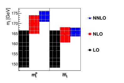
For illustration, we use the $\text{t}\bar{\text{t}}$ production cross section, measured in Ref. Kieseler (2015) at $\sqrt{s}=8\,\text{TeV}$, $\sigma=243.9\,\pm\,9.3\,\text{pb}$ to determine $\overline{m}_{t}$ and $m_{t}^{\text{p}}$ for different orders of perturbative QCD. The LHC beam-energy uncertainty of 1.72% is assigned to the predicted cross section, evaluated with the program HATHOR Aliev et al. (2011) based on calculations of Refs. Langenfeld et al. (2009); Bärnreuther et al. (2012); Czakon and Mitov (2012, 2013); Czakon et al. (2013). The cross section is calculated at LO, NLO, and next-to-next-to leading order (NNLO) accuracy with $\alpha_{S}$ at the Z-boson mass $M_{Z}$ set to $\alpha_{S}(M_{Z})=0.118\pm 0.001$ and is obtained using the parton distribution (PDF) set CT14 Dulat et al. (2015) evaluated at NNLO. Renormalization and factorization scales are set to $m_{t}^{\text{p}}$ or $\overline{m}_{t}$, respectively, and are varied independently by a factor of 2 up and down. The uncertainties due to variations of the CT14 PDF eigenvectors are scaled to 68% confidence level.

The extraction of $m_{t}^{\text{p}}$ and $\overline{m}_{t}$ is performed by comparison of predicted and measured $\sigma$. Experimental and theoretical uncertainties are considered uncorrelated. The resulting top-quark mass values are illustrated in Fig. 1. The scheme choice does not play a role at LO. When higher orders are considered in the calculation of $\sigma$, $\overline{m}_{t}$ exhibits a more rapid convergence than $m_{t}^{\text{p}}$.

Figure 1: Top-quark pole ($m_{t}^{\text{p}}$) and $\overline{{\text{MS}}}$ mass ($\overline{m}_{t}$) extracted from the inclusive $\text{t}\bar{\text{t}}$ production cross section by comparison with its prediction at different orders of perturbative QCD. The hatched areas indicate the total uncertainty on the measured mass values.

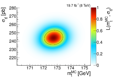
A detailed experimental analysis employing the method proposed here is documented in Ref. Kieseler (2015): the fit of $m_{t}^{\text{MC}}$ and $\sigma$ is performed simultaneously at center-of-mass energies of 7 and 8 TeV. As illustrated in Figure 2, the measured values are mostly uncorrelated.

Figure 2: Likelihood $L$ for the measured MC mass ($m_{t}^{\text{MC}}$) and $\text{t}\bar{\text{t}}$ production cross section ($\sigma_{t\bar{t}}$) at a center-of-mass energy of 8 TeV. The black contour corresponds to the 1 sigma uncertainty Kieseler (2015).

The obtained cross sections are compared to calculations with NNLO accuracy to determine $\overline{m}_{t}$. For the extraction of $m_{t}^{\text{p}}$, next-to-next-to leading log (NNLL) contributions are also accounted for. The measured $\overline{m}_{t}$ is converted to the pole mass $m_{t}^{\text{p,c}}$ in perturbation theory with up to four-loop accuracy in QCD Marquard et al. (2015). It is well-known that this leads to an additional positive shift of the value of $m_{t}^{\text{p}}$, the size of which indicates the residual theoretical uncertainty on $m_{t}^{\text{p}}$ at yet higher orders. For example, using a fixed $\overline{m}_{t}$ as input, the value of $m_{t}^{\text{p}}$ is approximately 0.5 GeV ​​(0.2 GeV) larger if the conversion formula is applied at three(four)-loop instead of two(three)-loop accuracy, respectively.

The results obtained at $\sqrt{s}=$ 7 and 8 TeV for $\overline{m}_{t}$, $m_{t}^{\text{p}}$, and $m_{t}^{\text{p,c}}$ are listed in Table 1 for different PDF sets Alekhin et al. (2014); Ball et al. (2015); Harland-Lang et al. (2015); Dulat et al. (2015). A strong correlation between the strong coupling constant, $\alpha_{S}$, and the measured top-quark mass can be observed.

	$\alpha_{S}(M_{Z})$	$\overline{m}_{t}$ [ GeV]	$m_{t}^{\text{p}}$ [ GeV]	$m_{t}^{\text{p,c}}$ [ GeV]
ABM12	0.113	$158.4\pm^{1.2}_{1.9}$	$166.6\pm^{1.6}_{1.9}$	$168.0\pm^{1.3}_{2.1}$
NNPDF3.0	0.118	$165.2\pm^{1.1}_{1.7}$	$174.0\pm^{1.4}_{1.7}$	$175.1\pm^{1.2}_{1.9}$
MMHT2014	0.118	$165.4\pm^{1.1}_{1.9}$	$174.3\pm^{1.4}_{1.8}$	$175.3\pm^{1.3}_{2.1}$
CT14	0.118	$165.5\pm^{1.5}_{2.0}$	$174.4\pm^{1.8}_{2.0}$	$175.4\pm^{1.7}_{2.2}$

Table 1: Measured $\overline{{\text{MS}}}$ ($\overline{m}_{t}$), pole ($m_{t}^{\text{p}}$), and pole mass from conversion ($m_{t}^{\text{p,c}}$) for different PDF sets and values for the strong coupling constant, $\alpha_{S}$, evaluated at the Z-boson mass, $M_{Z}$ Kieseler (2015).

All extracted values for ${m}_{{t}}$ are used to calibrate the $m_{t}^{\text{MC}}$ parameter, which is non-universal and, in principle, depends on the subtleties of its implementation in the MC simulation. In Ref. Kieseler (2015), $\bar{\Delta}_{m}=\overline{m}_{t}-m_{t}^{\text{MC}}$, $\Delta_{m}^{p}=m_{t}^{\text{p}}-m_{t}^{\text{MC}}$, and $\Delta_{m}^{p,c}=m_{t}^{\text{p,c}}-m_{t}^{\text{MC}}$ are calculated for $m_{t}^{\text{MC}}$ as implemented in MadGraph5 Alwall et al. (2011) interfaced with Pythia6 Sjöstrand et al. (2006) using the tune Z2^∗ Chatrchyan et al. (2013) and top-quark decays simulated with MadSpin2 Frixione et al. (2007). The results are listed in Table 2. A precision of about 2 GeV is achieved.

	$\bar{\Delta}_{m}$ [ GeV]	$\Delta_{m}^{p}$ [ GeV]	$\Delta_{m}^{p,c}$ [ GeV ]
ABM12	$-14.3\pm^{1.4}_{2.0}$	$-6.1\pm^{1.7}_{2.0}$	$-4.7\pm^{1.5}_{2.2}$
NNPDF3.0	$-7.6\pm^{1.3}_{1.9}$	$1.3\pm^{1.6}_{1.9}$	$2.4\pm^{1.5}_{2.0}$
MMHT2014	$-7.3\pm^{1.3}_{2.1}$	$1.5\pm^{1.6}_{2.0}$	$2.6\pm^{1.5}_{2.2}$
CT14	$-7.2\pm^{1.7}_{2.1}$	$1.6\pm^{1.9}_{2.1}$	$2.7\pm^{1.8}_{2.3}$

Table 2: Difference between the top quark mass in well-defined schemes and the top-quark MC mass for different PDF sets. The MC mass is compared to the $\overline{{\text{MS}}}$ mass ($\bar{\Delta}_{m}$), pole mass ($\Delta_{m}^{p}$), and the pole mass from conversion ($\Delta_{m}^{p,c}$) Kieseler (2015).

III Calibration with differential cross sections

An extension of the method to differential cross sections used for the determination of ${m}_{{t}}$ can provide a larger sensitivity and, possibly, a further reduction of systematic uncertainties. In the following, a differential production cross section for the signal process as a function of an observable $x$ is considered and employed to determine ${m}_{{t}}$. The approach used for $\sigma$ is applied to each bin of this differential cross section. For this purpose, the efficiency $\epsilon$ is replaced by a matrix $M$ describing the detector response to the predicted cross section $\sigma^{\text{MC}}_{k}$ in bin $k$ of the distribution in terms of $x$, defined by:

$${N}^{ps}_{j}=\mathcal{L}\cdot\sum_{k}M_{jk}{\sigma^{\text{MC}}_{k}}\text{,}$$ (3)

with ${N}^{ps}_{j}$ being the predicted number of reconstructed and selected signal events in bin $j$ of the reconstructed distribution. The response matrix is derived from MC simulation and therefore depends on $\vec{\lambda}$ as well as on $m_{t}^{\text{MC}}$ .

Each bin $j$ of the reconstructed distribution is considered as a category. In each category, a second observable $y$ is defined, sensitive to $m_{t}^{\text{MC}}$. The shape of this observable is used to constrain $m_{t}^{\text{MC}}$, while the total number of signal events in each category corresponds to ${N}^{ps}_{j}$, and hence can be used to derive the differential cross section. The number of predicted events, $N^{p}_{ij}$, in bin $i$ of the observable $y$ is given as:

$$N^{p}_{ij}=\mathcal{L}\cdot\sum_{k}M_{jk}(m_{t}^{\text{MC}},\vec{\lambda})\ {\sigma^{\text{MC}}_{k}}\cdot n_{ij}^{p}(m_{t}^{\text{MC}},\vec{\lambda})\\ +N^{bg}_{ij}(\vec{\lambda})\text{,}$$ (4)

with $n_{ij}^{p}$ being the fraction of predicted signal events in bin $i$ with respect to ${N}^{ps}_{j}$ and $N^{bg}_{ij}$ the contribution from background processes.

By comparison with the number of observed events $N_{ij}^{d}$ in each category $j$ and bin $i$, and considering $\sigma^{\text{MC}}_{k}\rightarrow\sigma_{k}$ as free parameters a fit can be performed maximizing the likelihood:

$$L(\sigma_{0},...,\sigma_{k},m_{t}^{\text{MC}},\vec{\lambda})=\prod_{i}\prod_{j}P\left(N^{p}_{ij},N^{d}_{ij}\right)\cdot\Xi(\vec{\lambda})\text{.}$$ (5)

This unfolding problem can be ill-posed and regularization techniques might need to be applied. A well-suited regularization condition is provided, for instance, by the aim to determine ${m}_{{t}}$ by comparison of $\sigma_{k}$ with its prediction $\sigma^{p}_{k}({m}_{{t}})$ as a function of ${m}_{{t}}$. Replacing $\sigma_{k}$ with this prediction corresponds to the folding approach used in Ref. CMS-PAS-TOP-14-014 (2014) and reduces the number of free parameters significantly, such that the likelihood becomes:

$$L({m}_{{t}},m_{t}^{\text{MC}},\vec{\lambda},\vec{\kappa})=\prod_{i}\prod_{j}P\left(N^{p}_{ij},N^{d}_{ij}\right)\cdot\Xi(\vec{\lambda},\vec{\kappa})\text{,}$$ (6)

with $\Xi(\vec{\lambda},\vec{\kappa})$ representing optional nuisance terms and $\vec{\kappa}$ being theoretical uncertainties on the predicted $\sigma^{p}_{k}({m}_{{t}})$. Both, $\vec{\lambda}$ and $\vec{\kappa}$ can be incorporated as nuisance terms in $\Xi$ or can be evaluated individually. In the latter case, $L$ depends on ${m}_{{t}}$ and $m_{t}^{\text{MC}}$, only. A maximization of $L$ directly returns the relation between these parameters as well as their correlations. The correlations are mainly incorporated through the response matrix $M$. Therefore, the event selection and the observable $x$ should be chosen such, that the dependence of $M$ on $m_{t}^{\text{MC}}$ is minimized and the sensitivity of $y$ on $m_{t}^{\text{MC}}$ becomes maximal.

For the optimization of the result, also the correlation between the observables $x$ and $y$ should be small. A possible choice for $x$ would be the differential $\text{t}\bar{\text{t}}$ production cross section as a function of the top-quark transverse momentum predicted up to NNLO accuracy Czakon et al. (2015). The dependence of this observable on $m_{t}^{\text{p}}$ and $\overline{m}_{t}$ can be studied at approximate NNLO with programs publicly available Guzzi et al. (2015). This distribution, describing the production dynamics, can be combined with an observable based on the kinematics of the decay products such as $m_{lb}$ in the dileptonic decay channel or the invariant mass of the 3 jets that originate from the top-quark decay $t\rightarrow Wb\rightarrow bq\bar{q}$ in the semileptonic channel.

The additional sensitivity of the differential cross sections to ${m}_{{t}}$ can result in uncertainties below 2 GeV on ${m}_{{t}}$ and $\Delta_{m}$, starting to challenge the measurements of $m_{t}^{\text{MC}}$ in precision and improving the understanding of this parameter. Moreover, determinations of the running of $\overline{m}_{t}(\mu)$ at varying scales $\mu$ as well as simultaneous extractions of the strong coupling $\alpha_{S}$ and ${m}_{{t}}$ become possible.

IV Conclusion

The simultaneous determination of $m_{t}^{\text{MC}}$ and of differential or inclusive production cross sections of processes sensitive to the top-quark mass ${m}_{{t}}$ allows for subsequent extraction of ${m}_{{t}}$ in a well-defined renormalization scheme. This method solves the longstanding problem of the calibration of the top-quark Monte Carlo mass $m_{t}^{\text{MC}}$ and, in addition, allows for a consistent quantification of the difference $\Delta_{m}={m}_{{t}}-m_{t}^{\text{MC}}$ for the particular MC tools used in the analysis and within the uncertainties of the measurement.

The extraction of ${m}_{{t}}$ is preferably performed in a scheme, where the perturbative expansion of the theory prediction for the respective cross section displays fast apparent convergence. For inclusive cross section, this applies to short-distance masses and favors an experimental determination of a running top-quark mass $\overline{m}_{t}$ over the pole mass $m_{t}^{\text{p}}$. The extracted $\overline{m}_{t}$ is more precise than $m_{t}^{\text{p}}$ obtained at the same order of perturbation theory and additional higher-order corrections result in smaller corrections to $\overline{m}_{t}$ than $m_{t}^{\text{p}}$. The latter can always be obtained up to four-loop accuracy in QCD.

With the current precision of the inclusive top-quark cross-section and mass measurements an uncertainty on $\Delta_{m}$ of approximately 2 GeV can be achieved. Dedicated analyses based on differential cross sections seem to be a promising approach to further decrease this uncertainty and to measure theoretically well-defined mass parameters independently of the interpretation of the top-quark MC mass to a high precision.

Acknowledgments
We would like to thank Olaf Behnke for useful discussions.

References

- Olive et al. (2014) K. A. Olive et al. (Particle Data Group), Chin. Phys. C38, 090001 (2014).
- Bezrukov et al. (2012) F. Bezrukov, M. Yu. Kalmykov, B. A. Kniehl, and M. Shaposhnikov, JHEP 10, 140 (2012), arXiv:1205.2893 [hep-ph] .
- Degrassi et al. (2012) G. Degrassi, S. Di Vita, J. Elias-Miro, J. R. Espinosa, G. F. Giudice, et al., JHEP 1208, 098 (2012), arXiv:1205.6497 [hep-ph] .
- Alekhin et al. (2012) S. Alekhin, A. Djouadi, and S. Moch, Phys. Lett. B716, 214 (2012), arXiv:1207.0980 [hep-ph] .
- Skands and Wicke (2007) P. Z. Skands and D. Wicke, Eur. Phys. J. C52, 133 (2007), arXiv:hep-ph/0703081 [hep-ph] .
- (2014) (ATLAS and CDF and CMS and D0 Collaborations) (ATLAS and CDF and CMS and D0 Collaborations), (2014), arXiv:1403.4427 [hep-ex] .
- Buckley et al. (2011) A. Buckley, J. Butterworth, S. Gieseke, D. Grellscheid, S. Höche, et al., Phys. Rept. 504, 145 (2011), arXiv:1101.2599 [hep-ph] .
- Hoang and Stewart (2008) A. H. Hoang and I. W. Stewart, Nucl. Phys. Proc. Suppl. 185, 220 (2008), arXiv:0808.0222 [hep-ph] .
- Moch et al. (2014) S. Moch et al., (2014), arXiv:1405.4781 [hep-ph] .
- (10) (CMS Collaboration), Measurement of the production cross section in the channel in pp collisions at 7 and 8 TeV, Tech. Rep. CMS-PAS-TOP-13-004 (CERN, Geneva, 2015).
- Aad et al. (2014) G. Aad et al. (ATLAS Collaboration), Eur. Phys. J. C74, 3109 (2014), arXiv:1406.5375 [hep-ex] .
- Aad et al. (2015a) G. Aad et al. (ATLAS Collaboration), JHEP 10, 121 (2015a), arXiv:1507.01769 [hep-ex] .
- Bigi et al. (1994) I. I. Y. Bigi, M. A. Shifman, N. G. Uraltsev, and A. I. Vainshtein, Phys. Rev. D50, 2234 (1994), arXiv:hep-ph/9402360 [hep-ph] .
- Beneke and Braun (1994) M. Beneke and V. M. Braun, Nucl. Phys. B426, 301 (1994), arXiv:hep-ph/9402364 [hep-ph] .
- Smith and Willenbrock (1997) M. C. Smith and S. S. Willenbrock, Phys. Rev. Lett. 79, 3825 (1997), arXiv:hep-ph/9612329 [hep-ph] .
- Hoang et al. (1999) A. H. Hoang, Z. Ligeti, and A. V. Manohar, Phys. Rev. D59, 074017 (1999), arXiv:hep-ph/9811239 [hep-ph] .
- Hoang and Teubner (1999) A. H. Hoang and T. Teubner, Phys. Rev. D60, 114027 (1999), arXiv:hep-ph/9904468 [hep-ph] .
- Beneke (1998) M. Beneke, Phys. Lett. B434, 115 (1998), arXiv:hep-ph/9804241 [hep-ph] .
- Langenfeld et al. (2009) U. Langenfeld, S. Moch, and P. Uwer, Phys. Rev. D80, 054009 (2009), arXiv:0906.5273 [hep-ph] .
- (20) (CMS Collaboration), Determination of the top-quark mass from the m(lb) distribution in dileptonic events at TeV, Tech. Rep. CMS-PAS-TOP-14-014 (CERN, Geneva, 2014).
- Aad et al. (2015b) G. Aad et al. (ATLAS Collaboration), Eur. Phys. J. C75, 330 (2015b), arXiv:1503.05427 [hep-ex] .
- Kieseler (2015) J. Kieseler, Measurement of Top-Quark Pair Production Cross Sections and Calibration of the Top-Quark Monte-Carlo Mass using LHC Run I Proton-Proton Collision Data at and 8 TeV with the CMS Experiment, Tech. Rep. DESY-THESIS-2015-054 (DESY, Hamburg, 2015).
- Aliev et al. (2011) M. Aliev, H. Lacker, U. Langenfeld, S. Moch, P. Uwer, et al., Comput. Phys. Commun. 182, 1034 (2011), arXiv:1007.1327 [hep-ph] .
- Bärnreuther et al. (2012) P. Bärnreuther, M. Czakon, and A. Mitov, Phys. Rev. Lett. 109, 132001 (2012), arXiv:1204.5201 [hep-ph] .
- Czakon and Mitov (2012) M. Czakon and A. Mitov, JHEP 1212, 054 (2012), arXiv:1207.0236 [hep-ph] .
- Czakon and Mitov (2013) M. Czakon and A. Mitov, JHEP 1301, 080 (2013), arXiv:1210.6832 [hep-ph] .
- Czakon et al. (2013) M. Czakon, P. Fiedler, and A. Mitov, Phys. Rev. Lett. 110, 252004 (2013), arXiv:1303.6254 [hep-ph] .
- Dulat et al. (2015) S. Dulat, T. J. Hou, J. Gao, M. Guzzi, J. Huston, et al., (2015), arXiv:1506.07443 [hep-ph] .
- Marquard et al. (2015) P. Marquard, A. V. Smirnov, V. A. Smirnov, and M. Steinhauser, Phys. Rev. Lett. 114, 142002 (2015), arXiv:1502.01030 [hep-ph] .
- Alekhin et al. (2014) S. Alekhin, J. Blümlein, and S. Moch, Phys. Rev. D 89, 054028 (2014), arXiv:1310.3059 [hep-ph] .
- Ball et al. (2015) R. D. Ball et al. (NNPDF), JHEP 04, 040 (2015), arXiv:1410.8849 [hep-ph] .
- Harland-Lang et al. (2015) L. A. Harland-Lang, A. D. Martin, P. Motylinski, and R. S. Thorne, Eur. Phys. J. C 75, 204 (2015), arXiv:1412.3989 [hep-ph] .
- Alwall et al. (2011) J. Alwall, M. Herquet, F. Maltoni, O. Mattelaer, and T. Stelzer, JHEP 1106, 128 (2011), arXiv:1106.0522 [hep-ph] .
- Sjöstrand et al. (2006) T. Sjöstrand, S. Mrenna, and P. Z. Skands, JHEP 0605, 026 (2006), arXiv:hep-ph/0603175 [hep-ph] .
- Chatrchyan et al. (2013) S. Chatrchyan et al. (CMS), JHEP 04, 072 (2013), arXiv:1302.2394 [hep-ex] .
- Frixione et al. (2007) S. Frixione, E. Laenen, P. Motylinski, and B. R. Webber, JHEP 04, 081 (2007), arXiv:hep-ph/0702198 [hep-ph] .
- Note (1) A more complete discussion of the response matrix can be found in Ref. CMS-PAS-TOP-14-014 (2014).
- Czakon et al. (2015) M. Czakon, D. Heymes, and A. Mitov, (2015), arXiv:1511.00549 [hep-ph] .
- Guzzi et al. (2015) M. Guzzi, K. Lipka, and S. Moch, JHEP 01, 082 (2015), arXiv:1406.0386 [hep-ph] .