Confluence of singularities in hypergeometric systems

Abstract

A system in a Birkhoff normal form with an irregular singularity of Poincaré rank 1 at the origin and a regular singularity at infinity is through the Borel-Laplace transform dual to a system in an Okubo form. Schäfke has showed that the Birkhoff system can also be obtained from the Okubo system by a simple limiting procedure. The Okubo system comes naturally with two kinds of mixed solution bases, both of which converge under the limit procedure to the canonical solutions of the limit Birkhoff system on sectors near the irregular singularity at the origin. One can then define Stokes matrices of the Okubo system as connection matrices between different branches of the mixed solution bases and use them to relate the monodromy matrices of the Okubo system to the usual Stokes matrices of the limit system at the irregular singularity. This is illustrated on the example of confluence in the generalized hypergeometric equation.

1 Introduction

A linear differential system

$$(s-B)\frac{dv}{ds}=(A+\rho)v,\qquad(s,v)\in\mathbb{CP}^{1}\times\mathbb{C}^{n},$$ (1)

where $A,B$ are constant $n\times n$-matrices, $B$ is diagonal, $\rho\in\mathbb{C}$ a parameter, is called an Okubo system, or also a hypergeometric system. Such systems appear as a natural generalization of the hypergeometric equation. It is known [Ko2], that every single Fuchsian differential equation can be reduced to such a system.

The assumption that $B$ is diagonal (or semisimple) assures that the 1-form $(s-B)^{-1}\,ds$ has only simple poles (placed at the eigenvalues of $B$ and at $\infty$), i.e. that all the singularities of the Okubo system (1) are Fuchsian.

The Okubo system (1) appears also as a dual to a system in Birkhoff normal form

$$z^{2}\frac{d\psi}{dz}=(B+zA)\psi,\qquad(z,\psi)\in\mathbb{CP}^{1}\times\mathbb{C}^{n},$$ (2)

which has an irregular singular point at 0 and a Fuchsian singular point at $\infty$, through the Laplace transform

$$\psi(z)=z^{-1-\rho}\int_{0}^{\infty}v(s,\rho)\,e^{-\frac{s}{z}}\,ds,\qquad|\arg s-\arg z|<\tfrac{\pi}{2}.$$

This fact can be used to express the Stokes and connection matrices of the Birkhoff system in terms of connection matrices and monodromies of the dual Okubo system [BJL, Sch1].

Schäfke [Sch2] has remarked that the the system (2) can be also obtained from (1) by the following confluence procedure:

$$\text{let}\quad s=\rho z,\quad\text{and}\quad y(z,\rho)=s^{-\rho}v(s,\rho),$$

then $y$ satisfies

$$z(z-\frac{1}{\rho}B)\frac{dy}{dz}=(B+zA)y,$$ (3)

which becomes (2) at the limit when $\rho\to\infty$.

In case of rank $n=2$ and $B$ with two distinct eigenvalues, this confluence procedure corresponds exactly to the confluence of the (Gauss’) hypergeometric equation to the (Kummer’s) confluent hypergeometric equation.

Aside from the usual local Levelt bases at each of the singularities, the Okubo system (1) has two other kinds of natural solution bases, so called mixed bases [BJL, Sch1, OTY]: The first one, called Floquet basis, consists of the Floquet solutions (singular Levelt solutions) at different finite singularities $\lambda_{j}$ (eigenvalues of $B$). The other, called co-Floquet basis, is in a sense dual; a co-Floquet solution at a singularity $\lambda_{j}$ is one that is analytic at al other singularities $\lambda_{k}$, $k\neq j$. Schäfke [Sch2] has studied the limits of these mixed bases in the confluent family (3) in the case where all the eigenvalues of $B$ are distinct and has shown that they both tend to the canonical solution basis of the limit system (Borel sum of a formal fundamental solution) on sectors at the irregular singularity $z=0$: the Floquet basis when $\rho\to+\infty$, and the co-Floquet basis when $\rho\to-\infty$.

This article exposes these results while extending them to a more general situation, where $B$ is allowed to have multiple eigenvalues, and $\rho$ can go to infinity along any fixed direction in one of two sectors of opening $>\pi$ covering a neighborhood of $\infty$ on the Riemann sphere $\mathbb{CP}^{1}$. In an analogy with [LR2, HLR] it is natural to introduce parametric Stokes matrices of the confluent family (3), as connection matrices between different branches of the Floquet (resp. co-Floquet) basis far from the origin. These parametric Stokes matrices are closely related to the monodromy of the family (3): in general, the monodromy matrices of the Floquet and co-Floquet bases can be expressed as products of these Stokes matrices and formal monodromy matrices. While the monodromy matrices diverge when $\rho\to\infty$ (because of their formal monodromy parts which are exponential functions of $\rho$) these parametric Stokes matrices tend to the usual Stokes matrices of the limit system, and can be easily obtained from them (Proposition 8 ).

These results are illustrated in Section 2 on explicit calculations in the case of the generalized hypergeometric equation, previously studied by Duval [Du]. Duval considered the problem of convergence of the monodromy matrices to the Stokes matrices without separating formal monodromy part and the Stokes part. Therefore she could only consider limits when $\rho\to\pm\infty$ following a discrete set of values on which the formal monodromy part is constant.

Remark 1.

A different confluence procedure of the type

$$(z^{2}-\epsilon)\frac{dy}{dz}=\Omega(z)y,\qquad\mathbb{C}\ni\epsilon\to 0,$$ (4)

was investigated in e.g. [Pa, Gl1, Gl2, LR2, HLR, Kl1, Kl2]. In case of $B$ having only two eigenvalues (one of which can be always shifted to 0), the confluence procedure (3) can be considered as a special case of (4). In this case our perspective essentially coincides with that of [LR2, HLR]. In particular, this includes the confluence in the Gauss’ hypergeometric equations [MR, Ra, Zh, LR1] and in the generalized hypergeometric equation [Du].

2 General theory

Let the matrix $B$ be diagonal with eigenvalues $\lambda_{1},\ldots,\lambda_{p}$ of respective multiplicities $n_{1},\dots,n_{p}$, and let the matrix $A$ be partitioned into blocks accordingly

$$B=\begin{pmatrix}\lambda_{1}I_{n_{1}}&&\\ &\ddots&\\ &&\lambda_{p}I_{n_{p}}\end{pmatrix},\qquad A=\begin{pmatrix}A_{11}&\ldots&A_{1p}\\ \vdots&&\vdots\\ A_{p1}&\ldots&A_{pp}\end{pmatrix}.$$

The following assumption is made throughout the text:

No two eigenvalues of $$A_{jj} 1\leq j\leq p$$ differ by a non-zero integer, . (5)

Notation 2.

For any $n\!\times\!n$-matrix $X$, let $(X_{ij})_{1\leq i,j\leq p}$ be its bloc-partition according to $B$, and denote  $X_{\cdot j}=$ the $j$-th bloc column of $X$.

2.1 Fundamental solution of the limit system (2)

It is well-known (see for example [Ba]) that the system (2) can be bloc-diagonalized by means of a formal power series transformation $\psi=\hat{T}(z)\phi$, with

$$\hat{T}(z)=\sum_{k=0}^{+\infty}T^{(k)}z^{k},\qquad T^{(0)}=0.$$

Under the assumption (5), the formally transformed system can be given the following Birkhoff form

$$z^{2}\frac{d\phi}{dz}=(B+zA_{D})\phi,\qquad\text{with}\quad A_{D}=\begin{pmatrix}A_{11}&&\\ &\ddots&\\ &&A_{pp}\end{pmatrix}.$$ (6)

Therefore the system (2) has a formal fundamental solution $\hat{\Psi}(z)$ whose $j$-th bloc-column is given by

$$\hat{\Psi}_{\cdot j}(z)=\hat{T}_{\cdot j}(z)z^{A_{jj}}e^{-\frac{\lambda_{j}}{z}}.$$

While $\hat{T}(z)$ is in general divergent, it is Borel summable. More precisely each its column $\hat{T}_{\cdot j}(z)$ is Borel summable in all directions $\alpha$ with $e^{i\alpha}\mathbb{R}^{+}$ disjoint from all $\lambda_{i}-\lambda_{j}$, $i\neq j$ (such direction $\alpha$ will be called non-singular). Let

$$U_{\cdot j}(s)=\sum_{k=0}^{+\infty}\frac{T^{(k)}_{\cdot j}}{k!}s^{k}$$ (7)

be the formal Borel transform of $z\,\hat{T}_{\cdot j}(z)$, convergent near $s=0$ and extended analytically on the universal covering of $\mathbb{C}\smallsetminus\{\lambda_{i}-\lambda_{j}\mid 1\leq i\leq p,\ i\neq j\}$. The matrix function $U(s)$ is a solution to linear system

$$s\frac{dU}{ds}-B\frac{dU}{ds}+\frac{dU}{ds}B=AU-U\!A_{D},$$

with Fuchsian singularities at the points $\lambda_{i}-\lambda_{j}$ and $\infty$. In particular, $U$ has only a moderate growth at each of the singularities. Therefore the Borel sum of $\hat{T}_{\cdot j}(z)$ in a non-singular direction $\alpha$ is well-defined by the Laplace integral

$$T_{[\alpha],\cdot j}(z)=\frac{1}{z}\int_{0}^{+\infty e^{i\alpha}}\!\!\!U_{\cdot j}(s)\,e^{-\frac{s}{z}}ds,$$

which converges and is bounded for $z$ in the open half-plane bisected by $e^{i\alpha}\mathbb{R}^{+}$, and whose value is independent of when the direction $\alpha$ varies a bit. In another words, the sectoral transformation $T_{[\alpha]}$ depends only on the homotopy class $[\alpha]$ of the direction $\alpha\in\mathbb{R}\smallsetminus\{\text{singular directions}\}$, and one can consider it as defined on a sector in the $z$-plane

$$\mathscr{S}_{[\alpha]}(\infty):=\bigcup_{\alpha^{\prime}\in[\alpha]}\{\Re(e^{-i\alpha^{\prime}}z)>0\},$$ (8)

of opening $>\pi$. Once a branch of $\log z$ is fixed, the system (2) has on each of these sectors a canonical solution basis $\Psi_{[\alpha]}(z)$

$$\Psi_{[\alpha],\cdot j}(z)=T_{[\alpha],\cdot j}(z)\,z^{A_{jj}}e^{-\frac{\lambda_{j}}{z}}=\frac{1}{z}\int_{0}^{+\infty e^{i\alpha}}\!\!\!U_{\cdot j}(s)\,e^{-\frac{s}{z}}ds\cdot z^{A_{jj}}e^{-\frac{\lambda_{j}}{z}}.$$ (9)

For every pair of non-singular directions $\alpha_{1},\,\alpha_{2}$ there is Stokes matrix $S_{[\alpha_{1}][\alpha_{2}]}(\infty)$

$$\Psi_{[\alpha_{2}]}=\Psi_{[\alpha_{1}]}\cdot S_{[\alpha_{1}][\alpha_{2}]}(\infty)$$ (10)

(defined by analytic continuation). It is an easy fact that for two neighboring direction classes $[\alpha_{1}],\,[\alpha_{2}]$ the Stokes matrix $S_{[\alpha_{1}][\alpha_{2}]}(\infty)$ is unipotent with only non-zero off-diagonal entries at the positions $(j,i)$ corresponding to the singularity $\lambda_{i}-\lambda_{j}$ separating the direction classes $[\alpha_{1}],\,[\alpha_{2}]$.

Remark 3.

Note that by the Liouville-Ostrogradski formula $\det T_{[\alpha]}$ is constant in $z$ and therefore equal to 1.

2.2 Fundamental solutions of the Okubo system

The Okubo system (1) has $(p+1)$ Fuchsian singularities on $\mathbb{CP}^{1}$ at the points $\lambda_{j}$, $1\leq j\leq p$, and $\infty$. Near each $s=\lambda_{j}$, the system is written as

$$(s-\lambda_{j})\frac{dv}{ds}=E_{j}(A+\rho)+{\cal O}(s-\lambda_{j}),$$

$E_{j}$ denoting the $j$-th column bloc of the identity matrix, and ${\cal O}(s\!-\!\lambda_{j})$ standing for holomorphic terms that vanish at $\lambda_{j}$. Its local “multipliers” are therefore $A_{jj}+\rho$ in the $j$-th bloc and $0$ in the other $(p-1)$ blocs.

The system comes with two kinds of canonical mixed bases that will be of interest in this article. The first one, which will be denoted $V^{+}$, consists of the so called Floquet solutions $V_{\cdot j}^{+}(s,\rho)$, which behave asymptotically like $E_{j}(s-\lambda_{j})^{A_{jj}+\rho}$ at the respective singularities $\lambda_{j}$. The second one, denoted by $V^{-}$, is in a sense dual to the Floquet basis; it consists of solutions $V_{\cdot j}^{-}(s,\rho)$ that are analytic at each other singularity $\lambda_{i}$, $i\neq j$. This section describes these two bases in more detail.

Definition 4.

Let $P^{+}$ be a sector at $\infty$ in the parameter $\rho$-space, on which $\arg\rho\in\,]\!-\!\pi+\eta,\pi-\eta[$, with $0<\eta<\frac{\pi}{2}$ fixed arbitrary, and $|\rho|$ is sufficiently big so that $\rho\notin-\mathbb{N}_{>0}-(\mathrm{Spec\,}A\cup\mathrm{Spec\,}A_{D})$.

Symmetrically, let $P^{-}$ be a sector at $\infty$ on which $\arg\rho\in\,]\eta,2\pi\!-\!\eta[$, and $|\rho|$ is sufficiently big so that $\rho\notin\mathbb{N}_{>0}-(\mathrm{Spec\,}A\cup\mathrm{Spec\,}A_{D})$.

The Floquet bases.

If $\Re(\rho)>0$ and $\rho$ is large enough so that all eigenvalues of $A_{jj}+\rho$ have positive real part, then the matrix function $(s-\lambda_{j})^{A_{jj}+\rho}$ vanishes when $s$ approaches $\lambda_{j}$ radially. Correspondingly, consider the space of solutions of (1) that vanish when $s\to\lambda_{j}$ radially. It is invariant by the local monodromy, and it follows from the local theory of Fuchsian singularities (cf. [IY, Le]) and the assumption (5) on $A_{jj}$, that this space has a unique basis written as

$$V_{\cdot j}^{+}(s,\rho)=(E_{j}+{\cal O}(s\!-\!\lambda_{j}))\cdot(s-\lambda_{j})^{A_{jj}+\rho}.$$ (11)

This construction can be extended to all parameters $\rho\in P^{+}$, if instead of letting $s$ approach $\lambda_{j}$ radially, one lets it approach $\lambda_{j}$ following a suitable logarithmic spiral along which $(s-\lambda_{j})^{A_{jj}+\rho}\to 0$. More precisely, $s$ should follow a real positive trajectory of the vector field $-e^{i\theta}(s\!-\!\lambda_{j})\partial_{s}$, for some $\theta\in\,]\!-\!\frac{\pi}{2},\frac{\pi}{2}[$ with $\Re(e^{i\theta}\rho)>0$.

The Floquet solution $V_{\cdot j}^{+}$ is closely related to the $j$-th formal canonical solution (9) of the dual Birkhoff system (2). In fact, the formal Borel transform (=term-wise inverse Laplace transform) of $z^{\rho+1}\hat{\Psi}_{\cdot j}(z)$ equals to the convolution integral [Sch1]

$$I_{\cdot j}^{+}(s,\rho):=\int_{\lambda_{j}}^{s}U_{\cdot j}(\sigma\!-\!\lambda_{j})(s\!-\!\sigma)^{A_{jj}+\rho-1}d\sigma\cdot\Gamma(A_{jj}\!+\!\rho)^{-1},$$ (12)

where the matricial Gamma function is defined as usual by the integral $\Gamma(A_{jj}+\rho)=\int_{0}^{+\infty}t^{-(A_{jj}+\rho-1)}e^{-t}dt,\,$ and $U(s)$ is given in (7). The integral (12), also known as Riemann-Liouville integral with base-point at $\lambda_{j}$, solves (1), and moreover it satisfies $\,\frac{d}{ds}I_{\cdot j}^{+}(s,\rho)=I_{\cdot j}^{+}(s,\rho-1)$, and therefore solves the difference equation

$$(s-B)I_{\cdot j}^{+}(s,\rho\!-\!1)=(A+\rho)I_{\cdot j}^{+}(s,\rho).$$

The canonical solution $\Psi_{[\alpha]}$ (9) of the Birkhoff system equals

$$\Psi_{[\alpha],\cdot j}(z)=z^{-\rho-1}\int_{\lambda_{j}}^{+\infty e^{i\alpha}}I_{\cdot j}^{+}(s,\rho)\,e^{-\frac{s}{z}}ds.$$ (13)

The Floquet solution $V_{\cdot j}^{+}$ is obtained from $I_{\cdot j}^{+}$ after a normalization:

$$V_{\cdot j}^{+}(s,\rho)=\int_{\lambda_{j}}^{s}U_{\cdot j}(\sigma\!-\!\lambda_{j})(s\!-\!\sigma)^{A_{jj}+\rho-1}d\sigma\cdot(A_{jj}\!+\!\rho).$$ (14)

The integrating path in (14) is such that $\sigma$ follows a positive real trajectory of the vector field $e^{i\theta}(s\!-\!\sigma)\partial_{\sigma}$ from the point $\lambda_{j}$ to $s$, with suitable $\theta$ as above, avoiding other singularities $\lambda_{i}$, $i\neq j$, of $U_{\cdot j}(\sigma-\lambda_{j})$. The set of points $s$ which can be reached by such paths with varying $\theta$ then defines a ramified domain on which (14) is defined. Note that if $\arg(s-\lambda_{j})=\alpha-\theta$, then the integrating trajectory approaches $\lambda_{j}$ in the asymptotic direction $\alpha$.

Let $\Omega^{+}_{[\alpha],j}(\rho)$ be a (ramified) domain consisting of those $s$ that can be reached by such trajectory for some direction $\alpha$ in the given homotopy class,

$$\Omega^{+}_{[\alpha],j}(\rho)\subseteq\{s\in\mathbb{C}\mid\arg(s-\lambda_{j})=\alpha^{\prime}-\theta,\ |\theta|<\tfrac{\pi}{2},\ |\theta+\arg\rho|<\tfrac{\pi}{2},\ \alpha^{\prime}\in[\alpha]\},$$

and let $\Omega^{+}_{[\alpha]}(\rho):=\bigcap_{j}\Omega^{+}_{[\alpha],j}(\rho)$. The restriction of $V^{+}$ to $\Omega^{+}_{[\alpha]}$ will be denoted $V_{[\alpha]}^{+}$. Different homotopy classes of non-singular directions $[\alpha]$ give rise to to different branches $V_{[\alpha]}^{+}$ of $V^{+}$ near infinity.

The co-Floquet bases.

For given index $j$, and a direction $\alpha$ such that $\lambda_{i}-\lambda_{j}\notin e^{i\alpha}\mathbb{R}^{+}$, $i\neq j$, define the co-Floquet solution $V_{[\alpha],\cdot j}^{-}$ at a singularity $\lambda_{j}$ as the unique solution analytic on $\mathbb{C}\smallsetminus\{\lambda_{j}+e^{i\alpha}\mathbb{R}^{+}\}$ and having the following asymptotic behavior near $\lambda_{j}$:

$$V_{[\alpha],\cdot j}^{-}(s,\rho)=(E_{j}+{O}(s\!-\!\lambda_{j}))\cdot(s\!-\!\lambda_{j})^{A_{jj}+\rho},$$ (15)

with $O$ denoting the usual Landau symbol (the corresponding terms may be ramified).

Let’s be more precise about where does it comes from. For each singularity $\lambda_{i}$ and $\rho\in P^{-}$ large enough so that $A_{ii}+\rho$ has no positive eigenvalue, define $\check{W}^{-}_{i}$ as the space of solutions analytic at $\lambda_{i}$. It follows from the local theory of Fuchsian singularities (cf. [IY, Le]) that this space is tangent exactly to the the $(p-1)$ vector-blocs $E_{k}$, $k\neq i$, corresponding to the multiplier 0. For a point $s\in\lambda_{j}-e^{i\alpha}\mathbb{R}^{+}$, continue each solution subspace $\check{W}^{-}_{i}$, $i\neq j$, toward $s$ in the cut plane $\mathbb{C}\smallsetminus\{\lambda_{j}+e^{i\alpha}\mathbb{R}^{+}\}$, and define the subspace $W_{\alpha,j}^{-}$ as their intersection. Since it consists of solutions analytic at each $\lambda_{k}$, $k\neq j$, it does not depend on the way the $\check{W}_{i}^{-}$ are continued around the singularities $\lambda_{k}$, only on the direction $\alpha$ of the cut.

Following [Sch1], there is a canonical bloc-solution of (1) generating the space $W_{\alpha,j}^{-}$ given by the integral:

$$I_{[\alpha]}^{-}(s,\rho):=\int_{\lambda_{j}}^{+\infty e^{i\alpha}}U_{\cdot j}(\sigma\!-\!\lambda_{j})(s\!-\!\sigma)^{A_{jj}+\rho-1}d\sigma\cdot\Gamma(1\!-\!A_{jj}-\rho)e^{-\pi i(A_{jj}+\rho)},$$ (16)

which satisfies again $\,\frac{d}{ds}I_{\cdot j}^{-}(s,\rho)=I_{\cdot j}^{-}(s,\rho-1)$, and therefore solves the difference equation

$$(s-B)I_{\cdot j}^{-}(s,\rho\!-\!1)=(A+\rho)I_{\cdot j}^{-}(s,\rho).$$ (17)

The integral $I_{[\alpha]}^{-}$ is a Laplace transform of the canonical solution $\Psi_{[\alpha]}$

$$I_{[\alpha]}^{-}(s,\rho):=\int_{0}^{+\infty e^{i\alpha}}z^{\rho-1}\Psi_{[\alpha],\cdot j}(z)e^{\frac{s}{z}}dz,$$

which in turn equals to

$$\Psi_{[\alpha],\cdot j}(z)=z^{-\rho-1}\frac{1}{2\pi i}\int_{\gamma_{j,\alpha}}I_{\cdot j}^{-}(s,\rho)\,e^{-\frac{s}{z}}ds,$$ (18)

where the path $\gamma_{j,\alpha}$ encircles the ray $\lambda_{j}+e^{i\alpha}\mathbb{R}^{+}$ in positive direction. While $\Psi_{[\alpha]}$ is defined on a sector at 0 of an opening $>\pi$ bisected by $e^{i\alpha}\mathbb{R}^{+}$, the integral $I_{[\alpha]}^{-}$ is defined on a sector at $\lambda_{j}$ bisected by $\lambda_{j}+e^{i(\alpha+\pi)}\mathbb{R}^{+}$ of an opening $>2\pi$.

The co-Floquet solution is obtained after a normalization

$$V_{[\alpha],\cdot j}^{-}(s,\rho)=\int_{\lambda_{j}}^{\infty}U_{\cdot j}(\sigma\!-\!\lambda_{j})(s\!-\!\sigma)^{A_{jj}+\rho-1}d\sigma\cdot(A_{jj}\!+\!\rho).$$ (19)

In the default situation when $\Re(\rho)<0$ the integration path is the straight ray $\sigma\in\lambda_{j}+e^{i\alpha}\mathbb{R}^{+}$ and the integral is defined for $s\in\lambda_{j}-e^{i\alpha}\mathbb{R}^{+}$ and extended analytically from there. In a general situation, the integration path follows a negative real trajectory of the vector field $e^{i\theta}(s\!-\!\sigma)\partial_{\sigma}$ from the point $\lambda_{j}$ to $\infty$, with a suitable $\theta\in\,]\!-\!\frac{\pi}{2},\frac{\pi}{2}[$ such that $\Re(e^{i\theta}\rho)<0$, that is end-point homotopic to the ray $\lambda_{j}+e^{i\alpha}\mathbb{R}^{+}$ in $\mathbb{CP}^{1}\smallsetminus\{\lambda_{i},\ i\neq j\}$. The set of points $s$ that can be reached by such paths defines again a (ramified) sectoral domain

$$\Omega^{-}_{[\alpha],j}(\rho)\subseteq\{s\in\mathbb{C}\mid\arg(s-\lambda_{j})=\alpha^{\prime}-\theta+\pi,\ |\theta|<\tfrac{\pi}{2},\ |\theta-\pi+\arg\rho|<\tfrac{\pi}{2},\alpha^{\prime}\in[\alpha]\},$$

on which the integral (19) is naturally defined. Let $\Omega^{-}_{[\alpha]}(\rho):=\bigcap_{j}\Omega^{-}_{[\alpha],j}(\rho)$.

Proposition 5.

For $\rho\in P^{+}\cap P^{-}$ and $s\in\lambda_{j}+e^{i\alpha}\mathbb{R}^{+}$, let $\tilde{s}=\lambda_{j}+e^{2\pi i}(s-\lambda_{j})$, then

$$V_{[\alpha],\cdot j}^{+}(s,\rho)=\big{[}V_{[\alpha],\cdot j}^{-}(\tilde{s},\rho)-V_{[\alpha],\cdot j}^{-}(s,\rho)\big{]}\cdot\big{[}e^{2\pi i(A_{jj}+\rho)}-1\big{]}^{-1},$$

or equivalently

$$I_{[\alpha],\cdot j}^{+}(s,\rho)=\frac{1}{2\pi i}\big{[}I_{[\alpha],\cdot j}^{-}(\tilde{s},\rho)-I_{[\alpha],\cdot j}^{-}(s,\rho)\big{]},$$

i.e. $I_{[\alpha],\cdot j}^{+}$ is a hyperfunction defined by the boundary value of $\frac{1}{2\pi i}I_{[\alpha],\cdot j}^{-}$ on $\lambda_{j}+e^{i\alpha}\mathbb{R}^{+}$.

Proof.

Follows from the construction. ∎

The following Proposition is due to Okubo and Kohno.

Proposition 6 (Gauss’–Kummer’s formula).

$$\det V_{[\alpha]}^{+}(s,\rho) =\frac{\det\Gamma(A_{D}+\rho+1)}{\det\Gamma(A+\rho+1)}\cdot\det\,(s-B)^{A_{D}+\rho},$$ (20)

$$\det V_{[\alpha]}^{-}(s,\rho) =\frac{\det\Gamma(-A-\rho)}{\det\Gamma(-A_{D}-\rho)}\cdot\det\,(s-B)^{A_{D}+\rho}.$$ (21)

Proof.

For the sake of completeness we will sketch here the proof in the co-Floquet case; the Floquet case is almost identical and can be found in [Ok1, Ko1, Ko2].

The co-Floquet solution has the following asymptotic behavior w.r.t. $\rho$ (see [Sch1], theorem (4.6)):

$$V_{[\alpha],\cdot j}^{-}(s,\rho)\cdot(s\!-\!\lambda_{j})^{-A_{jj}-\rho}=E_{j}+{O}(\frac{1}{|\rho|}),\quad\text{when }\ \Re(\rho)\to-\infty,$$ (22)

locally uniformly in the cut plane $\mathbb{C}\smallsetminus(\lambda_{j}+e^{i\alpha}\mathbb{R}^{+})$. Now, for $m\in\mathbb{N}$ it follows from (17) by induction that

$$I_{[\alpha],\cdot j}^{-}(s,\rho\!-\!m)\cdot(s\!-\!\lambda_{j})^{m}=(A\!+\!\rho\!-\!m\!+\!1)\cdots(A\!+\!\rho)\cdot I_{[\alpha],\cdot j}^{-}(s,\rho),$$

and hence

$$\Gamma(-A\!-\!\rho) \cdot\Gamma(-A\!-\!\rho\!+\!m)^{-1}\cdot V_{[\alpha],\cdot j}^{-}(s,\rho-m)\cdot(s\!-\!\lambda_{j})^{-A_{jj}-\rho+m}=$$

$$\qquad=V_{[\alpha],\cdot j}^{-}(s,\rho)\cdot(s\!-\!\lambda_{j})^{-A_{jj}-\rho}\cdot\Gamma(-A_{jj}\!-\!\rho)\cdot\Gamma(-A_{jj}\!-\!\rho+\!m)^{-1}.$$

Therefore

$$\frac{\det\Gamma(-A_{D}\!-\!\rho\!+\!m)}{\det\Gamma(-A\!-\!\rho\!+\!m)} \cdot\det\left[V_{[\alpha]}^{-}(s,\rho-m)\cdot(s\!-\!B)^{-A_{D}-\rho+m}\right]=$$

$$=\det\left[V_{[\alpha]}^{-}(s,\rho)\cdot(s\!-\!B)^{-A_{D}-\rho}\right]\cdot\frac{\det\Gamma(-A_{D}\!-\!\rho)}{\det\Gamma(-A\!-\!\rho)}.$$

Letting $m\to+\infty$ and using (22) and usual formulas for the $\Gamma$-function, one can see that both expressions on the left side tend to 1. ∎

Corollary 7.

For $\rho\in P^{+}$ (resp. $\rho\in P^{-}$) the Floquet (resp. the co-Floquet) solutions form a basis of the solution space.

2.3 Fundamental matrix solutions of the confluent family

The system (3) has two kinds of canonical fundamental matrix solutions $Y_{[\alpha]}^{\pm}(z,\rho)$ corresponding to the Floquet and co-Floquet bases of (2). In order to obtain a convergence when $\rho\to\infty$, one has to be a bit careful with the choice of their branch. It is convenient to write them as

$$Y_{[\alpha]}^{\pm}(z,\rho)=T_{[\alpha]}^{\pm}(z,\rho)\cdot\Phi(z,\rho),$$ (23)

where

$$\Phi(z,\rho):=z^{-\rho}(z-\tfrac{B}{\rho})^{A_{D}+\rho},$$

is a canonical solution to the bloc-diagonal system

$$z(z-\tfrac{B}{\rho})\frac{d\phi}{dz}=(B+zA_{D})\phi,$$ (24)

whose branch needs to be selected so that it converges to the adequate branch of

$$\Phi(z,\infty):=z^{A_{D}}e^{-\frac{B}{z}},$$

when $\rho\to\infty$. The bloc-diagonalizing transformation $T_{[\alpha]}^{\pm}$ is defined by

$$T_{[\alpha]}^{\pm}(z,\rho)=V_{[\alpha]}^{\pm}(\rho z,\rho)\cdot(\rho z-B)^{-A_{D}-\rho},$$

where the branch of $(\rho z-B)^{-A_{D}-\rho}$ is chosen in accord with the one inside the integral (14), (19). Hence

$$T_{[\alpha],\cdot j}^{+}(z,\rho)=\int_{0}^{\rho z-\lambda_{j}}U_{\cdot j}(\sigma)\Big{(}\frac{\rho z-\lambda_{j}-\sigma}{\rho z-\lambda_{j}}\Big{)}^{A_{jj}+\rho}\frac{d\sigma}{\rho z-\lambda_{j}-\sigma}\cdot(A_{jj}+\rho),$$ (25)

where the integration path follows a positive trajectory of the vector field $\,e^{i\theta}(\rho z\!-\!\lambda_{j}\!-\!\sigma)\partial_{\sigma}$ from the point 0 to $\rho z\!-\!\lambda_{j}$, and the branch of $\Big{(}\frac{\rho z-\lambda_{j}-\sigma}{\rho z-\lambda_{j}}\Big{)}^{A_{jj}+\rho}$ is chosen so that it is equal 1 at the endpoint. Remark, that at the limit, when $\rho\to\infty$ radially with fixed $\arg\rho$, the trajectories of the given vector field become trajectories of the vector field $e^{i\alpha}\partial_{z}$ with $\alpha=\theta+\arg\rho+\arg z$. Therefore the integral (25) has a well-defined limit

$$T_{[\alpha],\cdot j}^{+}(z,\infty)=\frac{1}{z}\int_{0}^{+\infty e^{i\alpha}}U_{\cdot j}(\sigma)\,e^{-\frac{\sigma}{z}}d\sigma.$$

Similarly,

$$T_{[\alpha],\cdot j}^{-}(z,\rho)=\int_{0}^{\infty}U_{\cdot j}(\sigma)\Big{(}\frac{\rho z-\lambda_{j}-\sigma}{\rho z-\lambda_{j}}\Big{)}^{A_{jj}+\rho}\frac{d\sigma}{\rho z-\lambda_{j}-\sigma}\cdot(A_{jj}+\rho),$$ (26)

where the integration path follows a positive trajectory of $\,e^{i\theta-\pi}(\rho z\!-\!\lambda_{j}\!-\!\sigma)\partial_{\sigma}$ from the point 0 to $\infty$, which at the limit, when $\rho\to\infty$ radially, becomes a trajectory of $\,e^{i\alpha}\partial_{z}$ with $\alpha=\theta+\arg\rho-\pi+\arg z$, and the integral (26) becomes

$$T_{[\alpha],\cdot j}^{-}(z,\infty)=\frac{1}{z}\int_{0}^{+\infty e^{i\alpha}}U_{\cdot j}(\sigma)\,e^{-\frac{\sigma}{z}}d\sigma.$$

The transformations $T_{[\alpha]}^{\pm}(\cdot,\rho)$ are defined on sectors

$$\mathscr{S}_{[\alpha]}^{\pm}(\rho):=\tfrac{1}{\rho}\Omega^{\pm}_{[\alpha]}(\rho),$$

which tend to a subsector of $\mathscr{S}_{[\alpha]}(\infty)$ (8) depending on the radial direction in which $\rho\to\infty$.

Stokes matrices of the confluent family

Fixing a branch of $\Phi(z,\rho)$ near $z=\infty$ and its restrictions to the sectors $\mathscr{S}_{[\alpha]}^{\pm}(\rho)$ one obtains a canonical set of fundamental matrix solutions $Y_{[\alpha]}^{\pm}(z,\rho)$ (23). The connection matrices between these solutions near $z=\infty$ corresponding to different non-singular directions $\alpha_{1},\,\alpha_{2}$

$$Y_{[\alpha_{2}]}^{\pm}=Y_{[\alpha_{1}]}^{\pm}\cdot S_{[\alpha_{1}][\alpha_{2}]}^{\pm}(\rho)$$

will be called Stokes matrices of the family.

Proposition 8.

$$S_{[\alpha_{1}][\alpha_{2}]}^{+}(\rho) =\rho^{A_{D}}\Gamma(A_{D}+\rho+1)^{-1}S_{[\alpha_{1}][\alpha_{2}]}(\infty)\,\Gamma(A_{D}+\rho+1)\rho^{-A_{D}},$$

$$S_{[\alpha_{1}][\alpha_{2}]}^{-}(\rho) =\big{(}e^{-\pi i}\rho\big{)}^{-A_{D}}\Gamma(-A_{D}-\rho)\,S_{[\alpha_{1}][\alpha_{2}]}(\infty)\,\Gamma(-A_{D}-\rho)^{-1}\big{(}e^{-\pi i}\rho\big{)}^{-A_{D}},$$

which tends to the Stokes matrix $S_{[\alpha_{1}][\alpha_{2}]}(\infty)$ (10) when $\rho\to\infty$ in $P^{\pm}$ respectively. For two neighboring direction classes $[\alpha_{1}],\,[\alpha_{2}]$ the Stokes matrix $S_{[\alpha_{1}][\alpha_{2}]}^{\pm}(\rho)$ is unipotent with only non-zero off-diagonal blocs at the positions $(i,j)$ corresponding to the direction of $(\lambda_{i}-\lambda_{j})\mathbb{R}+$ separating $\alpha,\,\alpha^{\prime}$.

Proof.

This follows from the relation

$$I_{[\alpha_{2}]}^{\pm}(s,\rho)=I_{[\alpha_{1}]}^{\pm}(s,\rho)\cdot S_{[\alpha_{1}][\alpha_{2}]}^{\pm}(\rho),$$

which is a consequence of the formulas (13), resp. (18). ∎

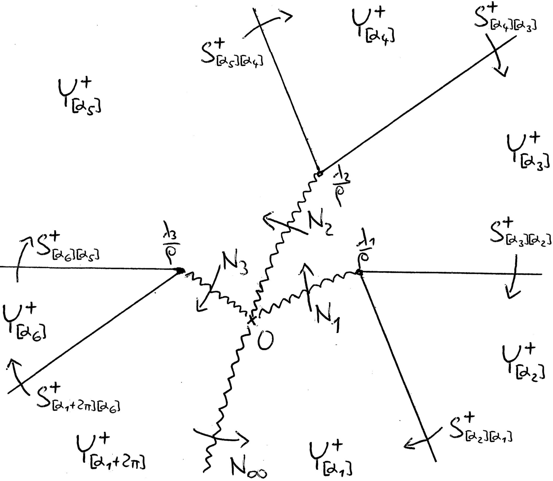
(a) $\rho\in\mathbb{R}+$

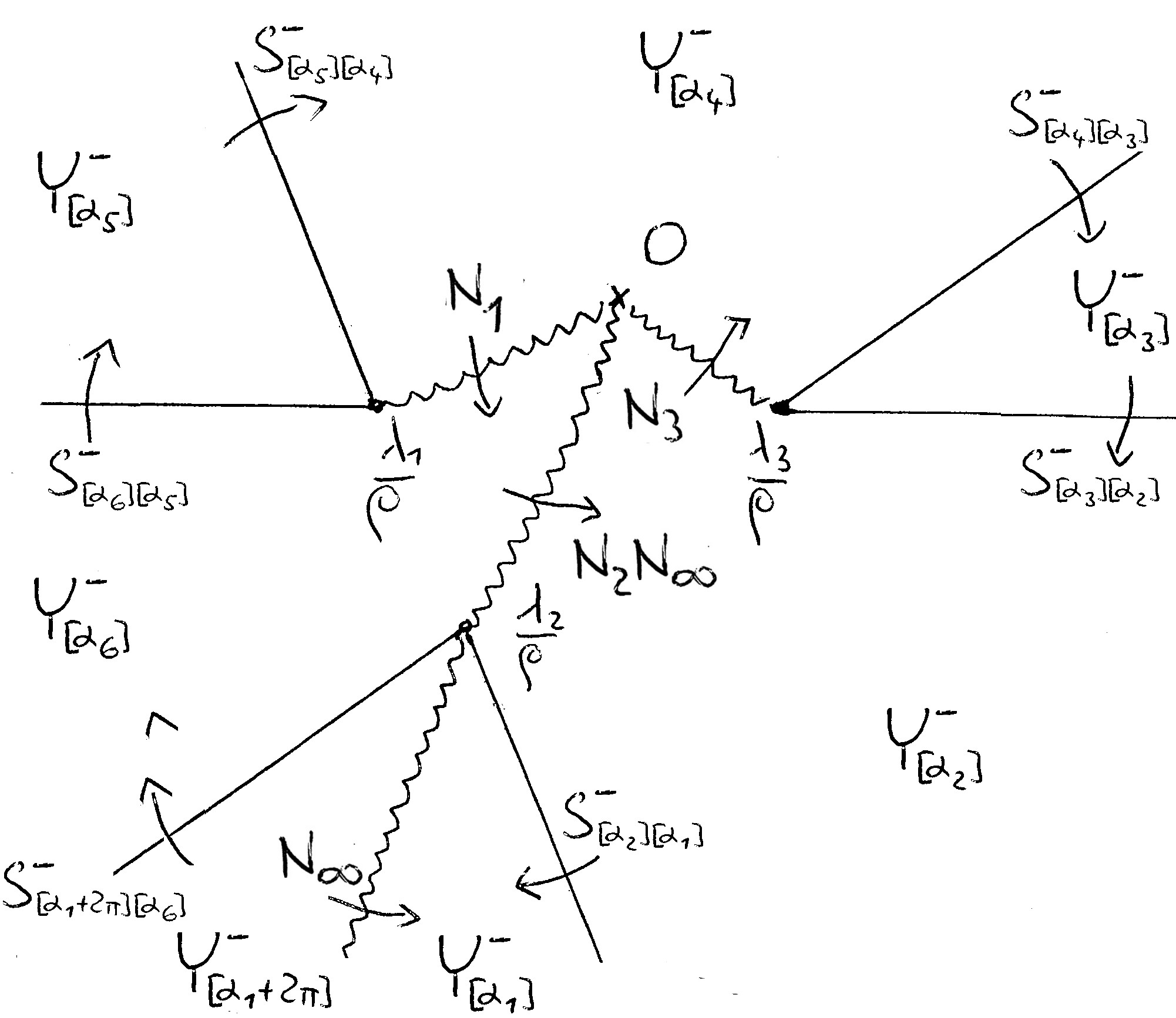
(b) $\rho\in\mathbb{R}-$

Figure 1: The connection matrices between different branches of $Y^{\pm}$ in Example 9.

Example 9 (Figure 1).

Suppose $B$ has just three eigenvalues $\lambda_{i}$, $i=1,2,3$ and assume they are not colinear. For simplicity we will consider only the default situation when $\rho\in\mathbb{R}\pm$ and restrict the domains of $Y_{[\alpha]}^{\pm}$ to a smaller sector consisting of the points $z\in\mathbb{C}$ for which the integration path in (25), resp. (26), can be taken a straight segment. Near $\infty$, these sectors are are separated by the outer parts of lines through $\lambda_{i},\lambda_{k}$, whose crossing is governed by the Stokes matrices. For each singularity $\frac{\lambda_{j}}{\rho}$ or $\infty$ make a cut (wavy line in Figure 1) from the origin on which the formal solution $\Phi$ is branched, and therefore changed by its formal monodromy

$$N_{j}=\left(\begin{smallmatrix}I_{n_{1}}\hskip-3.0pt&&&&\\[-6.0pt] &\ddots&&&\\[1.0pt] &&\hskip-12.0pte^{2\pi i(A_{jj}+\rho)}\hskip-18.0pt&&\\[-4.0pt] &&&\ddots&\\ &&&&I_{n_{3}}\end{smallmatrix}\right),\quad j=1,2,3,\quad\text{and}\quad N_{\infty}=e^{-2\pi iA_{D}}.$$

3 Confluence in generalized hypergeometric equation

This section illustrates the confluence procedure on the example of the generalized hypergeometric equation, where things can be expressed very explicitly. Most of the formulas come from [Du, OTY, Lu]. To simplify the writing we adopt the following notation.

Notation 10.

Let $\bm{\alpha}=(\alpha_{1},\ldots,\alpha_{n})$, $\bm{\beta}=(\beta_{1},\ldots,\beta_{n})\in\mathbb{C}^{n}$ and denote

• $\hat{\bm{\beta}}{\raisebox{2.0pt}{${}^{\,j}$}}\in\mathbb{C}^{n-1}$ obtained from $\bm{\beta}$ by omitting the $j$-th component, similarly with $\hat{\bm{\beta}}{\raisebox{2.0pt}{${}^{n,j}$}}\in\mathbb{C}^{n-2}$,

• for $c\in\mathbb{C}$, let $\,\bm{\alpha}-c:=(\alpha_{1}-c,\ldots,\alpha_{n}-c),$

• for a function $f:\mathbb{C}\to\mathbb{C}$, write shortly $\,f(\bm{\alpha}):=\displaystyle\Pi_{i}f(\alpha_{i}).$

In the above notation, the generalized hypergeometric equation of order $n$, is written as $\displaystyle D\Big{(}\genfrac{.}{.}{0.0pt}{}{\bm{\alpha}}{\bm{\beta}}\Big{|}\,s\Big{)}w=0$, where

$$D\Big{(}\genfrac{.}{.}{0.0pt}{}{\bm{\alpha}}{\bm{\beta}}\Big{|}\,s\Big{)}: =s(\delta_{s}+\alpha_{n})\ldots(\delta_{s}+\alpha_{1})-(\delta_{s}+\beta_{n}\!-\!1)\ldots(\delta_{s}+\beta_{1}\!-\!1)$$

$$=s(\delta_{s}+\bm{\alpha})-(\delta_{s}+\bm{\beta}-1),$$ (27)

and $\delta_{s}=s\frac{d}{ds}$ is the Euler operator. It has three regular singular points at $0$, $1$ and $\infty$.

Since

$$D\Big{(}\genfrac{.}{.}{0.0pt}{}{\bm{\alpha}}{\bm{\beta}}\Big{|}\,s\Big{)}(s^{c}w)=s^{c}D\Big{(}\genfrac{.}{.}{0.0pt}{}{\bm{\alpha}\!+\!c}{\bm{\beta}\!+\!c}\Big{|}\,s\Big{)}w,$$ (28)

one can always use the transformation $w\mapsto s^{1-\beta_{j}}w$, to bring the equation to a more usual form in which one of the $\beta_{j}$’s equals 1: $\displaystyle D\Big{(}\genfrac{.}{.}{0.0pt}{}{\bm{\alpha}\!+\!1\!-\!\beta_{j}}{\bm{\beta}\!+\!1\!-\!\beta_{j}}\Big{|}\,s\Big{)}$. The equation (3) has thus $n$ local solution at $s=0$ given by the hypergeometric series

$$s^{1-\beta_{j}}{}_{n}F_{n-1}\Big{(}\genfrac{.}{.}{0.0pt}{}{\bm{\alpha}\!+\!1\!-\!\beta_{j}}{\hat{\bm{\beta}}{\raisebox{2.0pt}{${}^{j}$}}\!+\!1\!-\!\beta_{j}}\Big{|}\,s\Big{)}:=s^{1-\beta_{j}}\sum_{k=0}^{+\infty}\frac{(\bm{\alpha}\!+\!1\!-\!\beta_{j})_{k}}{(\hat{\bm{\beta}}{\raisebox{2.0pt}{${}^{j}$}}\!+\!1\!-\!\beta_{j})_{k}(1)_{k}}s^{k},\quad 1\leq j\leq n,$$

convergent for $|s|<1$, where $(a)_{k}$ denotes the Pochhammer symbol

$$(a)_{k}=a\,(a\!+\!1)\ldots(a\!+\!k\!-\!1),\quad(a)_{0}=1.$$

These solutions are linearly independent if no two $\beta_{j}$’s differ by an integer.

Remark 11.

There is a symmetry between the singular points $0$ and $\infty$ given by the relation

$$D\Big{(}\genfrac{.}{.}{0.0pt}{}{\bm{\alpha}}{\bm{\beta}}\Big{|}\,s\Big{)}=(-1)^{n}s\,D\Big{(}\genfrac{.}{.}{0.0pt}{}{1\!-\!\bm{\beta}}{1\!-\!\bm{\alpha}}\Big{|}\,\frac{1}{s}\Big{)}.$$ (29)

In the case of the Gauss’ hypergeometric equation ($n=2$) there is also a symmetry between the two singular points $0,1$ due to the relation

$$D\Big{(}\genfrac{.}{.}{0.0pt}{}{\alpha_{1},\alpha_{2}}{1,\beta}\Big{|}\,s\Big{)}=\frac{s}{1\!-\!s}D\Big{(}\genfrac{.}{.}{0.0pt}{}{\alpha_{1},\alpha_{2}}{1,-\gamma}\Big{|}\,1\!-\!s\Big{)},\qquad\gamma=\beta\!-\!1\!-\!\alpha_{1}\!-\!\alpha_{2}.$$

This symmetry is broken for $n>2$.

The confluence.

We are interested in the situation when $\beta_{n}\to\infty$. The situation when $\alpha_{n}\to\infty$ would be similar due to the symmetry (29). Let

$$\rho=\beta_{n}-1,\qquad s=\rho z$$

then

$$\tfrac{1}{\rho}D\Big{(}\genfrac{.}{.}{0.0pt}{}{\bm{\alpha}}{\bm{\beta}}\Big{|}\,\rho z\Big{)}=z(\delta_{z}+\bm{\alpha})-(\tfrac{1}{\rho}\delta_{z}+1)(\delta_{z}+\hat{\bm{\beta}}{\raisebox{2.0pt}{${}^{n}$}}-1),$$ (30)

where the regular singularities at $z=0$ and $z=\frac{1}{\rho}$ merge for $\rho\to\infty$ to form an irregular singularity.

Setting $y=(y_{1},\ldots,y_{n})^{\mathsf{T}}$, with

$$y_{i+1}(z,\rho)=(\delta_{z}+\beta_{i}\!-\!1)y_{i}(z,\rho),\quad\text{for}\quad 1\leq i\leq n\!-\!1,$$

the equation (30): $\,\displaystyle\tfrac{1}{\rho}D\Big{(}\genfrac{.}{.}{0.0pt}{}{\bm{\alpha}}{\bm{\beta}}\Big{|}\,\rho z\Big{)}y_{1}=0\,$ is written in the form of a family of systems (3) with

$$B=\begin{pmatrix}0&&&\\[-3.0pt] &\ddots&&\\ &&0&\\ &&&1\end{pmatrix},\qquad A=\begin{pmatrix}1\!-\!\beta_{1}\hskip-9.0pt&\hskip 6.0pt1\hskip-6.0pt&&\\[-3.0pt] &\ddots&\ddots&\\ &&\hskip-12.0pt1\!-\!\beta_{n-1}\hskip-6.0pt&1\\ *&\ldots&*&\gamma\end{pmatrix},$$ (31)

$$\gamma:=\sum_{1}^{n-1}(\beta_{j}\!-\!1)-\sum_{1}^{n}\alpha_{n},$$

where $A$ has $-\alpha_{1},\ldots,-\alpha_{n}$ as eigenvalues.

The Okubo system.

The corresponding Okubo system

$$(s-B)\frac{dv}{ds}=(A+\rho)v$$ (32)

for $v(s,\rho)=s^{-\rho}y(z,\rho)$, is associated to the generalized hypergeometric equation

$$D\Big{(}\genfrac{.}{.}{0.0pt}{}{\bm{\alpha}\!-\!\rho}{\bm{\beta}\!-\!\rho}\Big{|}\,s\Big{)}v_{1}(s,\rho)=0,\qquad v_{i+1}(s,\rho)=(\delta_{s}+\beta_{i}\!-\!1\!-\!\rho)v_{i}(s,\rho).$$

Suppose now, that

$$\beta_{i}-\beta_{j}\notin\mathbb{Z}\ \text{ for all }i\neq j.$$ (33)

For $\rho\neq\infty$, we have $n-1$ singular solutions of the Okubo system near $s=0$ whose first component is given by

$$\tilde{v}_{1j}^{+}(s,\rho)=s^{1-\beta_{j}+\rho}\,{}_{n}F_{n-1}\Big{(}\genfrac{.}{.}{0.0pt}{}{\bm{\alpha}\!+\!1\!-\!\beta_{j}}{\hat{\bm{\beta}}{\raisebox{2.0pt}{${}^{j}$}}\!+\!1\!-\!\beta_{j}}\Big{|}\,s\Big{)},\qquad|s|<1,\quad 1\leq j\leq n-1,$$

and one singular solution at $s=1$ given by Meijer G-function

$$\tilde{v}_{1n}^{+}(s,\rho) =G_{n,n}^{n,0}\Big{(}\genfrac{.}{.}{0.0pt}{}{\bm{\beta}}{\bm{\alpha}}\Big{|}\,\frac{1}{z}\Big{)}\cdot\Gamma(1\!+\!\gamma\!+\!\rho),\qquad|s|>1,$$

$$=(s\!-\!1)^{\gamma+\rho}\sum_{k=0}^{+\infty}\frac{(-1)^{k}c_{k}}{(\gamma+\rho+1)_{k+n-1}}(s\!-\!1)^{k+n-1},\qquad|s-1|<1,$$

with $c_{0}=1$ and the coefficients $c_{k}$ independent of $\rho$ (see [Du], p. 601)

$$\,c_{k}=\text{\footnotesize{$\displaystyle\sum_{i_{1}+\ldots+i_{n-1}=k}\prod_{j=1}^{n-1}\frac{(\beta_{1}\!-\alpha_{1}\!+i_{1}+\ldots+\beta_{j}\!-\alpha_{j}\!+i_{j})_{i_{j}}\cdot(\beta_{j}\!-\!\alpha_{j+1})_{i_{j}}}{i_{j}!}$}}.$$ (34)

It is easy to see that the terms of the fundamental solution matrix $\tilde{V}^{+}=(\tilde{v}_{ij}^{+})$ have the asymptotic behavior

$$\tilde{V}^{+}(s,\rho)\sim\left(R+O(1)(s-B)\right)(s-B)^{\tilde{A}_{D}+\rho},$$

where the upper-triangular matrix $R=(r_{ij})$

$$r_{1j}=1,\quad r_{ij}=(\beta_{1}\!-\!\beta_{j})\ldots(\beta_{i-1}\!-\!\beta_{j}),\ i>1,\quad\text{and}\quad r_{nn}=1,\quad r_{in}=0,\ i<n,$$

commutes with $B$ and diagonalizes

$$A_{D}=\begin{pmatrix}1\!-\!\beta_{1}\hskip-9.0pt&\hskip 3.0pt1\hskip-6.0pt&&&\\[-8.39996pt] &\raisebox{1.79993pt}{$\ddots$}&\hskip-3.0pt\raisebox{8.39996pt}{$\ddots$}&\hskip-12.0pt1&\\ &&&\hskip-24.0pt1\!-\!\beta_{n-1}\hskip-6.0pt&\\ &&&&\,\gamma\end{pmatrix},\qquad R^{-1}\!A_{D}R=\tilde{A}_{D}:=\begin{pmatrix}1\!-\!\beta_{1}\hskip-9.0pt&\hskip 3.0pt&&\\[-3.0pt] &\ddots&&\\ &&\hskip-12.0pt1\!-\!\beta_{n-1}\hskip-6.0pt&\\ &&&\,\gamma\end{pmatrix}.$$

Therefore,

$$V^{+\!}(s,\rho)=\tilde{V}^{+\!}(s,\rho)R^{-1}$$ (35)

is the Floquet bases of the Okubo system (32) with the asymptotic behavior (11), while $R^{-1}\tilde{V}^{+}$ is the Floquet basis of the Okubo system with $\tilde{B}=B$, $\tilde{A}=R^{-1}AR$.

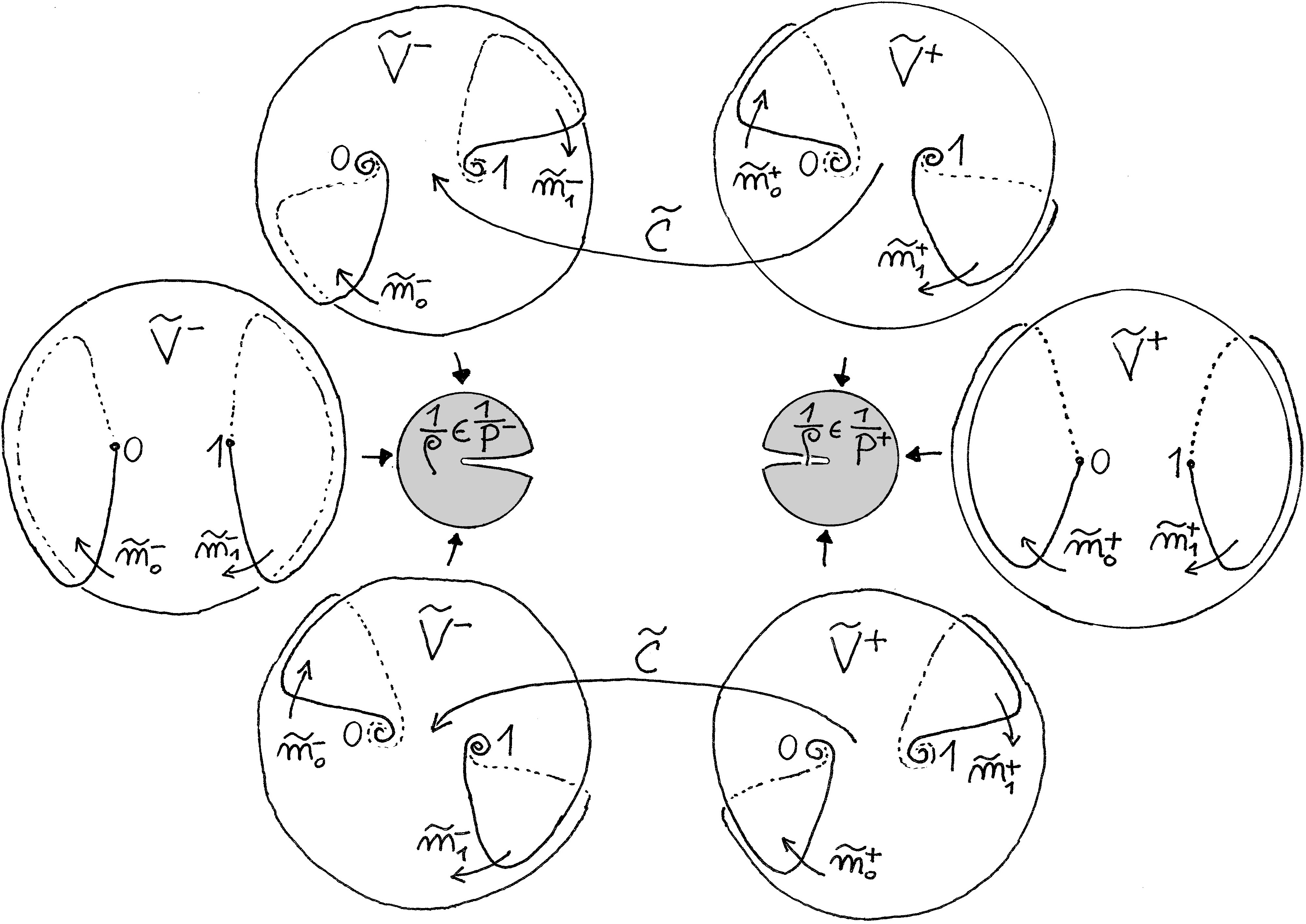
Figure 2: The fundamental matrix solutions $\tilde{V}^{\pm}$ and their monodromy and transition matrices, according to the values of $\frac{1}{\rho}$.

Monodromy matrices $\tilde{m}_{0}^{+}(\rho)$ and $\tilde{m}_{1}^{+}(\rho)$ of the solution $\tilde{V}^{+}$ around the singularities $0$ and $1$ in the positive direction from a base-point at $s=\frac{1}{2}$ are calculated in [OTY]:

$$\tilde{m}_{0}^{+}=\begin{pmatrix}e_{1}&&&\xi_{1}(e_{1}\!-\!1)\\[-3.0pt] &\hskip-6.0pt\ddots&&\vdots\\ &&\hskip-6.0pte_{n-1}\hskip-3.0pt&\xi_{n-1}(e_{n-1}\!-\!1)\hskip-3.0pt\\[3.0pt] &&&1\end{pmatrix},\qquad\tilde{m}_{1}^{+}=\begin{pmatrix}1&&&\\[-3.0pt] &\ddots&&\\ &&\hskip-6.0pt1&\\[3.0pt] \eta_{1}(e_{n}\!-\!1)\hskip-4.0pt&\ldots&\hskip-4.0pt\eta_{n-1}(e_{n}\!-\!1)\hskip-4.0pt&e_{n}\end{pmatrix},$$

where $\,e_{j}=e^{2\pi i(1-\beta_{j}+\rho)},\,\text{ for }\,j\leq n-1,\,\ e_{n}=e^{2\pi i(\gamma+\rho)},\,$ and

$$\xi_{j}=e^{\pi i(\gamma+\rho)}\frac{\Gamma(1\!+\!\gamma\!+\!\rho)\Gamma(\beta_{j}\!-\!\hat{\bm{\beta}}{\raisebox{2.0pt}{${}^{j}$}})}{\Gamma(\beta_{j}\!-\!\bm{\alpha})},\qquad\eta_{j}=e^{-\pi i(\gamma+\rho)}\frac{\Gamma(\!-\gamma\!-\!\rho)\Gamma(1\!-\!\beta_{j}\!+\!\hat{\bm{\beta}}{\raisebox{2.0pt}{${}^{j}$}})}{\Gamma(1\!-\!\beta_{j}\!+\!\bm{\alpha})}.$$

The connection matrix between the Floquet and the co-Floquet bases $\tilde{V}^{-}(s,\rho)=\tilde{V}^{+}(s,\rho)\tilde{C}(\rho)$ is also calculated in [OTY]:

$$\tilde{C}=\begin{pmatrix}1&&&\hskip-6.0pt-\xi_{1}\\[-3.0pt] &\ddots&&\vdots\\ &&\hskip-6.0pt1&\hskip-6.0pt-\xi_{n-1}\hskip-3.0pt\\[3.0pt] -\eta_{1}\hskip-3.0pt&\ldots&\hskip-3.0pt-\eta_{n-1}\hskip-6.0pt&1\end{pmatrix}.$$

Therefore the corresponding monodromy matrices of $\tilde{V}^{-}$ are equal to

$$\tilde{m}_{\iota}^{-}(\rho)=\tilde{C}(\rho)^{-1}\tilde{m}_{\iota}^{+}(\rho)\tilde{C}(\rho),\quad\iota=0,1,$$

$$\tilde{m}_{0}^{-}=\begin{pmatrix}e_{1}\hskip-12.0pt&&&\\[-3.0pt] &\hskip-6.0pt\ddots&&\\ &&\hskip-20.0pte_{n-1}&\\[3.0pt] \eta_{1}(e_{1}\!-\!1)\hskip-4.0pt&\ldots&\hskip-4.0pt\eta_{n-1}(e_{n-1}\!-\!1)\hskip-4.0pt&1\end{pmatrix},\qquad\tilde{m}_{1}^{-}=\begin{pmatrix}1&&&\xi_{1}(e_{n}\!-\!1)\\[-3.0pt] &\ddots&&\vdots\\ &&1&\xi_{n-1}(e_{n}\!-\!1)\hskip-3.0pt\\[3.0pt] &&&e_{n}\end{pmatrix}.$$

Remark 12.

The Floquet and co-Floquet bases $\tilde{V}^{\pm}$ are both defined and analytic not only on $\rho\in P^{\pm}$ but for all $\rho\in\mathbb{C}$ except of a discrete set of resonant values accumulating at $\infty$.

The confluent family.

Under the assumption (33) there are $n\!-\!1$ parameter-dependent singular solutions of the confluent equation (30) near $z=0$ are given for $\rho\neq\infty$ by

$$\tilde{y}_{1j}^{+}(z,\rho) =z^{1-\beta_{j}}\,{}_{n}F_{n-1}\Big{(}\genfrac{.}{.}{0.0pt}{}{\bm{\alpha}\!+\!1\!-\!\beta_{j}}{\hat{\bm{\beta}}{\raisebox{2.0pt}{${}^{j}$}}\!+\!1\!-\!\beta_{j}}\Big{|}\,\rho z\Big{)}$$

$$=z^{1-\beta_{j}}\,G_{n,n}^{n,1}\Big{(}\genfrac{.}{.}{0.0pt}{}{1,\,\hat{\bm{\beta}}{\raisebox{2.0pt}{${}^{j}$}}\!+\!1\!-\!\beta_{j}}{\bm{\alpha}\!+\!1\!-\!\beta_{j}}\Big{|}\,\!-\frac{1}{\rho z}\Big{)}\cdot\frac{\Gamma(\hat{\bm{\beta}}{\raisebox{2.0pt}{${}^{j}$}}\!+\!1\!-\!\beta_{j})}{\Gamma(\bm{\alpha}\!+\!1\!-\!\beta_{j})},\qquad|\rho z|<1,$$

$$\downarrow$$

$$\tilde{y}_{1j}^{+}(z,\infty) =z^{1-\beta_{j}}\,G_{n-1,n}^{n,1}\Big{(}\genfrac{.}{.}{0.0pt}{}{1,\,\hat{\bm{\beta}}{\raisebox{2.0pt}{${}^{n,j\!}$}}\!+\!1\!-\!\beta_{j}}{\bm{\alpha}\!+\!1\!-\!\beta_{j}}\Big{|}\,\!-\frac{1}{z}\Big{)}\cdot\frac{\Gamma(\hat{\bm{\beta}}{\raisebox{2.0pt}{${}^{n,j\!}$}}\!+\!1\!-\!\beta_{j})}{\Gamma(\bm{\alpha}\!+\!1\!-\!\beta_{j})},\quad|\arg z-\pi|<\frac{3\pi}{2},$$

with the limit asymptotic on compact sub-sectors to the divergent formal series

$$z^{1-\beta_{j}}\,{}_{n}F_{n-2}\Big{(}\genfrac{.}{.}{0.0pt}{}{\bm{\alpha}\!+\!1\!-\!\beta_{j}}{\hat{\bm{\beta}}{\raisebox{2.0pt}{${}^{n,j\!}$}}\!+\!1\!-\!\beta_{j}}\Big{|}\,z\Big{)}=z^{1-\beta_{j}}\,\sum_{k=0}^{+\infty}\frac{(\bm{\alpha}\!+\!1\!-\!\beta_{j})_{k}}{(\hat{\bm{\beta}}{\raisebox{2.0pt}{${}^{n,j}$}}\!+\!1\!-\!\beta_{j})_{k}(1)_{k}}z^{k}.$$

And the singular solution at $z=\frac{1}{\rho}$ is is given by

$$\tilde{y}_{1n}^{+}(z,\rho) =G_{n,n}^{n,0}\Big{(}\genfrac{.}{.}{0.0pt}{}{\bm{\beta}}{\bm{\alpha}}\Big{|}\,\frac{1}{\rho z}\Big{)}\cdot\rho^{-\gamma}\,\Gamma(1\!+\!\gamma\!+\!\rho),\qquad|\rho z|>1$$

$$\downarrow$$

$$\tilde{y}_{1n}^{+}(z,\infty) =G_{n-1,n}^{n,0}\Big{(}\genfrac{.}{.}{0.0pt}{}{\hat{\bm{\beta}}{\raisebox{2.0pt}{${}^{n}$}}}{\bm{\alpha}}\Big{|}\,\frac{1}{z}\Big{)},\qquad|\arg z|<\frac{3\pi}{2},$$

which is asymptotic on compact sub-sectors to the divergent formal series

$$e^{-\frac{1}{z}}z^{\gamma}\sum_{k=0}^{+\infty}(-1)^{k}c_{k}z^{k+n-1},\qquad\text{with $c_{k}$ as in \eqref{eq:hg-ck}.}$$

The constructed fundamental matrix solution $\tilde{Y}^{+}=(\tilde{y}_{ij}^{+})$ have the asymptotic behavior

$$\tilde{Y}^{+}(z,\rho)\sim\left(R+O(1)(z-\tfrac{B}{\rho})\right)(z-\tfrac{B}{\rho})^{\tilde{A}_{D}+\rho}z^{-\rho}.$$

Therefore

$$Y^{+\!}(z,\rho):=\tilde{Y}^{+\!}(z,\rho)R^{-1}\sim\left(I+O(1)(z-\tfrac{B}{\rho})\right)(z-\tfrac{B}{\rho})^{A_{D}+\rho}z^{-\rho}$$

is the corresponding Floquet bases of the confluent family (31) with the right asymptotic behavior.

In the definition of $\tilde{Y}^{+}$ above the right choice of branch of $\log z$ and $\log(z-\frac{1}{\rho})$ in $\tilde{\Phi}(z,\rho)=(z-\tfrac{B}{\rho})^{\tilde{A}_{D}+\rho}z^{-\rho}$ is of essential importance. Let $\alpha$ be a direction, $-\pi<\alpha<0$, and chose the bases $\tilde{Y}^{\pm}_{[\alpha]}$ and $\tilde{Y}^{\pm}_{[\alpha+\pi]}$ so that they are related to each other as in Figure 3,

$$\tilde{Y}_{[\alpha+\pi]}^{+}(z,\rho)=(\rho z)^{-\rho}\tilde{V}^{+}(\rho z,\rho)\rho^{-\tilde{A}_{D}},\quad\tilde{Y}_{[\alpha]}^{-}(z,\rho)=(\rho z)^{-\rho}\tilde{V}^{-}(\rho z,\rho)\rho^{-\tilde{A}_{D}}.$$

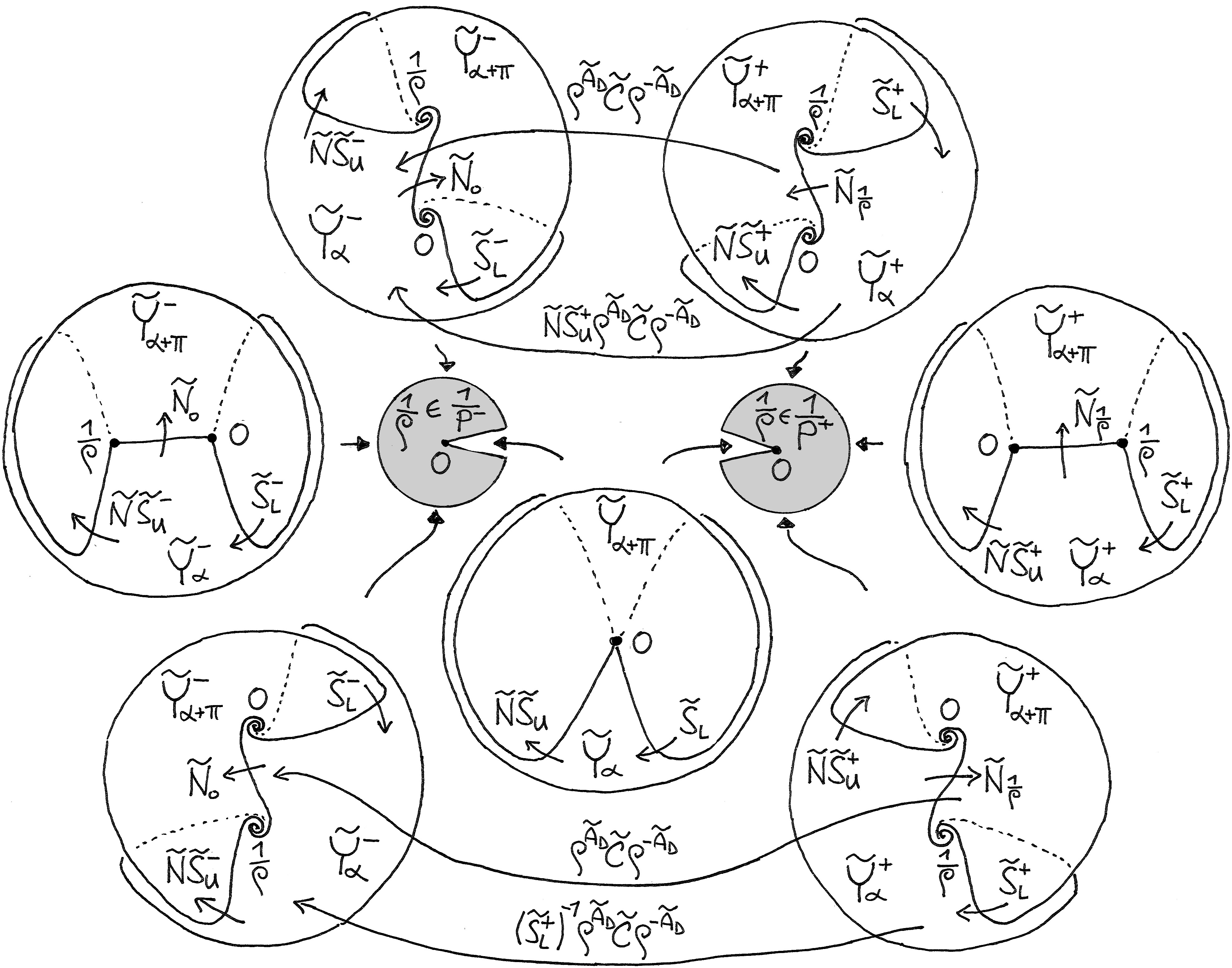
Figure 3: The fundamental matrix solutions $\tilde{Y}^{\pm}_{[\alpha]}$, $\tilde{Y}^{\pm}_{[\alpha+\pi]}$ on their natural domains (restricted to a fixed neighborhood of 0) and their transition matrices, according to the values of $\frac{1}{\rho}$. The limit system is in the center. (See [LR2, HLR, Kl2] for more details on the construction of these ramified domains.)

Then the monodromy matrices of the fundamental matrix solution $\tilde{Y}_{[\alpha+\pi]}^{+}(z,\rho)$, resp. $\tilde{Y}_{[\alpha]}^{-}(z,\rho)$, around $0$ and $\frac{1}{\rho}$ ($\rho\neq\infty$) in the positive direction from a base-point at $z=\frac{1}{2\rho}$ are equal

$$\tilde{M}_{0}^{+}=\tilde{N}_{0}\tilde{S}_{U}^{+}=e^{-2\pi i\rho}\rho^{\tilde{A}_{D}}\tilde{m}^{+}_{0}\rho^{-\tilde{A}_{D}},\qquad\tilde{M}_{\frac{1}{\rho}}^{+}=\tilde{S}_{L}^{+}\tilde{N}_{\frac{1}{\rho}}=\rho^{\tilde{A}_{D}}\tilde{m}^{+}_{1}\rho^{-\tilde{A}_{D}},$$ (36)

resp.

$$\tilde{M}_{0}^{-}=\tilde{N}_{0}\tilde{S}_{L}^{-}=e^{-2\pi i\rho}\rho^{\tilde{A}_{D}}\tilde{m}^{-}_{0}\rho^{-\tilde{A}_{D}},\qquad\tilde{M}_{\frac{1}{\rho}}^{-}=\tilde{N}\tilde{S}_{U}^{-}\tilde{N}_{0}^{-1}=\rho^{\tilde{A}_{D}}\tilde{m}^{-}_{1}\rho^{-\tilde{A}_{D}},$$ (37)

where

$$\tilde{N}_{0}=\begin{pmatrix}e^{2\pi i(1-\beta_{1})}\hskip-18.0pt&&&\\[-3.0pt] &\hskip-6.0pt\ddots&&\\ &&e^{2\pi i(1-\beta_{n-1})}\hskip-24.0pt&\\ &&&e^{-2\pi i\rho}\end{pmatrix},\qquad\tilde{N}_{\frac{1}{\rho}}=\begin{pmatrix}1&&&\\[-3.0pt] &\ddots&&\\ &&1&\\ &&&e^{2\pi i(\gamma+\rho)}\end{pmatrix},$$

and $\,\tilde{N}=\tilde{N}_{0}\tilde{N}_{\frac{1}{\rho}},\,$ are monodromies of the fundamental matrix solution $\tilde{\Phi}(z,\rho)=z^{-\rho}(z-\frac{B}{\rho})^{\tilde{A}_{D}+\rho}$ of the diagonal model system, and

$$\tilde{S}_{U}^{\pm}:=\tilde{S}_{\alpha+2\pi,\alpha+\pi}^{\pm}=\begin{pmatrix}1&&&\tilde{s}^{\pm}_{1n}\ \\[-3.0pt] &\hskip-3.0pt\ddots\hskip-3.0pt&&\hskip 3.0pt\vdots\ \\ &&1\hskip-6.0pt&\tilde{s}^{\pm}_{n-1,n}\hskip-3.0pt\\[3.0pt] &&&1\end{pmatrix},\qquad\tilde{S}_{L}^{\pm}:=\tilde{S}_{\alpha+\pi,\alpha}^{\pm}=\begin{pmatrix}1&&&\\[-3.0pt] &\ddots&&\\ &&\hskip-6.0pt1&\\[3.0pt] \tilde{s}^{\pm}_{n1}\hskip-6.0pt&\ldots&\hskip-6.0pt\tilde{s}^{\pm}_{n,n-1}\hskip-6.0pt&1\end{pmatrix}$$

are the Stokes matrices. It follows from (36) that the Stokes multipliers $\tilde{s}^{+}_{ij}(\rho)$ are equal to:

$$\tilde{s}^{+}_{jn}(\rho) =\xi_{j}(\rho)\,(1\!-\!e^{-2\pi i(\rho+1-\beta_{j})})\,\rho^{1-\beta_{j}-\gamma}$$

$$=-2\pi i\,e^{\pi i(\gamma+\beta_{j}+n)}\frac{\Gamma(\beta_{j}\!-\!\hat{\bm{\beta}}{\raisebox{2.0pt}{${}^{n,j}$}})}{\Gamma(\beta_{j}\!-\!\bm{\alpha})}\cdot\rho^{1-\beta_{j}-\gamma}\frac{\Gamma(1\!+\!\gamma\!+\!\rho)}{\Gamma(2\!-\!\beta_{j}\!+\!\rho)},$$

$$\downarrow$$

$$\tilde{s}^{+}_{jn}(\infty) =-2\pi i\,e^{\pi i(\gamma+\beta_{j}+n)}\frac{\Gamma(\beta_{j}\!-\!\hat{\bm{\beta}}{\raisebox{2.0pt}{${}^{n,j}$}})}{\Gamma(\beta_{j}\!-\!\bm{\alpha})},$$

$\big{(}\,\text{since}\ \lim_{P^{+}\ni\rho\to\infty}\rho^{\gamma+\beta_{j}-1}\frac{\Gamma(2-\beta_{j}+\rho)}{\Gamma(1+\gamma+\rho)}=1\,\big{)},$ and

$$\tilde{s}^{+}_{nj}(\rho) =\eta_{j}(\rho)\,(e^{2\pi i(\gamma+\rho)}\!-\!1)\,\rho^{\gamma+\beta_{j}-1}$$

$$=-2\pi i\frac{\Gamma(1\!-\!\beta_{j}\!+\!\hat{\bm{\beta}}{\raisebox{2.0pt}{${}^{n,j}$}})}{\Gamma(1\!-\!\beta_{j}\!+\!\bm{\alpha})}\cdot\rho^{\gamma+\beta_{j}-1}\frac{\Gamma(2\!-\!\beta_{j}\!+\!\rho)}{\Gamma(1\!+\!\gamma\!+\!\rho)},$$

$$\downarrow$$

$$\tilde{s}^{+}_{nj}(\infty) =-2\pi i\frac{\Gamma(1\!-\!\beta_{j}\!+\!\hat{\bm{\beta}}{\raisebox{2.0pt}{${}^{n,j}$}})}{\Gamma(1\!-\!\beta_{j}\!+\!\bm{\alpha})}.$$

From (37) one then obtains the Stokes multipliers $\tilde{s}^{-}_{ij}(\rho)$:

$$\tilde{s}^{-}_{jn}(\rho) =\xi_{j}(\rho)\,e^{-2\pi i(1-\beta_{j}+\rho)}(e^{2\pi i(\gamma+\rho)}\!-\!1)\,\rho^{1-\beta_{j}-\gamma}$$

$$=-2\pi i\,e^{\pi i(\gamma+\beta_{j}+n)}\frac{\Gamma(\beta_{j}\!-\!\hat{\bm{\beta}}{\raisebox{2.0pt}{${}^{n,j}$}})}{\Gamma(\beta_{j}\!-\!\bm{\alpha})}\cdot\left(e^{-\pi i}\rho\right)^{1-\beta_{j}-\gamma}\frac{\Gamma(\beta_{j}\!-\!1\!-\!\rho)}{\Gamma(\!-\gamma\!-\!\rho)},$$

$$\downarrow$$

$$\tilde{s}^{-}_{jn}(\infty) =-2\pi i\,e^{\pi i(\gamma+\beta_{j}+n)}\frac{\Gamma(\beta_{j}\!-\!\hat{\bm{\beta}}{\raisebox{2.0pt}{${}^{n,j}$}})}{\Gamma(\beta_{j}\!-\!\bm{\alpha})},$$

$\big{(}\,\text{since}\ \lim_{P^{-}\ni\rho\to\infty}(e^{-\pi i}\rho)^{\gamma+\beta_{j}-1}\frac{\Gamma(-\gamma-\rho)}{\Gamma(\beta_{j}-1-\rho)}=1\,\big{)}$, and

$$\tilde{s}^{-}_{nj}(\rho) =\eta_{j}(\rho)\,(e^{2\pi i(1-\beta_{j}+\rho)}\!-\!1)\,\rho^{\gamma+\beta_{j}-1}$$

$$=-2\pi i\frac{\Gamma(1\!-\!\beta_{j}\!+\!\hat{\bm{\beta}}{\raisebox{2.0pt}{${}^{n,j}$}})}{\Gamma(1\!-\!\beta_{j}\!+\!\bm{\alpha})}\cdot\left(e^{-\pi i}\rho\right)^{\gamma+\beta_{j}-1}\frac{\Gamma(\!-\gamma\!-\!\rho)}{\Gamma(\beta_{j}\!-\!1\!-\!\rho)},$$

$$\downarrow$$

$$\tilde{s}^{-}_{nj}(\infty) =-2\pi i\frac{\Gamma(1\!-\!\beta_{j}\!+\!\hat{\bm{\beta}}{\raisebox{2.0pt}{${}^{n,j}$}})}{\Gamma(1\!-\!\beta_{j}\!+\!\bm{\alpha})}.$$

One could also proceed the opposite way: The Stokes matrices $\tilde{S}_{\bullet}(\infty)$, $\bullet=U,L$, of the limit generalized confluent hypergeometric equation have been calculated in [DM, KO], and the Stokes matrices $\tilde{S}_{\bullet}^{\pm}(\rho)$ of the family are related to them via Proposition 8.

Note that the confluent Floquet and co-Floquet bases $Y^{\pm}(z,\rho)=\tilde{Y}^{\pm}(z,\rho)R^{-1}$ and their monodromies, resp. Stokes matrices $M_{i}^{\pm}(\rho)=R\tilde{M}_{i}^{\pm}(\rho)R^{-1}$, $\iota=0,\frac{1}{\rho}$, resp. $S_{\bullet}^{\pm}(\rho)=R\tilde{S}_{\bullet}^{\pm}(\rho)R^{-1}$, $\bullet=U,L$, are well-defined under a weaker assumption than (33), that no two $\beta_{j}$’s differ by a non-zero integer.

References

• [Ba] W. Balser, Formal power series and linear systems of meromorphic ordinary differential equations, Springer, 2000.
• [BJL] W. Balser, W.B. Jurkat, D.A. Lutz, On the reduction of connection problems with an irregular singularity to ones with only regular singularities, I, II, SIAM J. Math. Anal. 12 (1981), 691–721, SIAM J. Math. Anal. 19 (1988), 398–443.
• [Du] A. Duval, Confluence procedures in the generalized hypergeometric family, J. Math. Sci. Univ. Tokyo 5 (1998), 597–625.
• [DM] A. Duval, C. Mitschi, Matrices de Stokes et groupe de Galois des équations hypergéométriques généralisées, Pacific J. of Math. 138 (1989), 25–56.
• [Gar] R. Garnier, Sur les singularités irrégulières des équations différentielles linéaires, J. de math. pures et appl. $8^{e}$ série (1919), 99–200.
• [Gl1] A. Glutsyuk, Stokes Operators via Limit Monodromy of Generic Perturbation, J. Dyn. Control Syst. 5 (1999), 101–135.
• [Gl2] A. Glutsyuk, Resonant Confluence of Singular Points and Stokes Phenomena, J. Dyn. Control Syst. 10 (2004), 253–302.
• [Hu] M. Hukuhara, Développements Asymptotiques des Solutions Principales d’un Systeme Différentiel Linéaire du Type Hypergéométrique, Tokyo J. of Math. 05 (1982), 491–499.
• [HLR] J. Hurtubise, C. Lambert, C. Rousseau, Complete system of analytic invariants for unfolded differential linear systems with an irregular singularity of Poincaré rank k, Moscow Math. J. 14 (2013), 309–338.
• [IY] Y. Ilyashenko, S. Yakovenko, Lectures on Analytic Differential Equations, Grad. Studies Math. 86, Amer. Math. Soc., Providence, 2008.
• [Kl1] M. Klimeš, Analytic classification of families of linear differential systems unfolding a resonant irregular singularity, preprint arXiv:1301.5228.
• [Kl2] M. Klimeš, Confluence of singularities of non-linear differential equations via Borel-Laplace transformations, to be published in J. Dynam. Contr. Syst. [arXiv:1307.8383]
• [Ko1] M. Kohno, Frobenius’ theorem and Gauss-Kummer’s formula, Funkcialaj Ekvacioj 28 (1985), 249–266.
• [Ko2] M. Kohno, Global analysis in linear differential equations, Math. and its appl. 471, Kluwer Acad. Publ., Dodrecht, 1999.
• [KO] M. Kohno, S. Ohkohchi, Generalized hypergeometric equations of non-Fuchsian type, Hiroshima Math. J. 13 (1983), 83–100.
• [Le] A.H.M. Levelt, Hypergeometric functions, dissertation, Nederl. Akad. Wetensch. Proc. Ser. A 64, 1961.
• [LR1] C. Lambert, C. Rousseau, The Stokes phenomenon in the confluence of the hypergeometric equation using Riccati equation, J. Differential Equations 244 (2008) 2641-–2664.
• [LR2] C. Lambert, C. Rousseau, Complete system of analytic invariants for unfolded differential linear systems with an irregular singularity of Poincaré rank 1, Moscow Math. Journal 12 (2012), 77–138.
• [Lu] Y.L. Luke, Special functions and their approximations I, II, Math. Sci. Eng. 53, Acad. Press, New York, 1969.
• [MR] J. Martinet, J.-P. Ramis, Théorie de Galois differentielle et resommation, in: Computer Algebra and Differential Equations (E.Tournier ed.), Acad. Press (1988).
• [Ok1] K. Okubo, An Extension of Gauss’ Formula for Hypergeometric Series, 数理解析研究所講究録 105 (1971), 53–57. [http://hdl.handle.net/2433/106318]
• [Ok2] K. Okubo, Connection problems for systems of linear differential equations, Lect. Notes in Math. 243, Springer, 1971.
• [OTY] K. Okubo, K. Takano, S. Yoshida, A connection problem for the generalized hypergeometric equation, Funkcialaj Ekvacioj 31 (1988), 483–495.
• [Pa] L. Parise, Confluence de singularités régulières d’équations différentielles en une singularité irrégulière. Modèle de Garnier, thèse de doctorat, IRMA Strasbourg (2001). [http://www-irma.u-strasbg.fr/annexes/publications/pdf/01020.pdf]
• [Ra] J.-P. Ramis, Confluence et résurgence, J. Fac. Sci. Univ. Tokyo, Sec. IA Math. 36 (1989), 703–716.
• [Sch1] R. Schäfke, Über das globale analytische Verhalten der Normallösungen von $(s-B)v^{\prime}(s)=(B+t^{-1}A)v(s)$ und zweier Arten von assoziierten Funktionen, Math. Nachr. 121 (1985), 123–145.
• [Sch2] R. Schäfke, Confluence of several regular singular points into an irregular singular one, J. Dyn. Control Syst. 4 (1998), 401–424.
• [Zh] C. Zhang, Confluence et phenomène de Stokes, J. Math. Sci. Univ. Tokyo 3 (1996), 91–107.