Momentum-Resolved and Correlations Spectroscopy Using Quantum Probes

Abstract

We address some key conditions under which many-body lattice models, intended mainly as simulated condensed matter systems, can be investigated via immersed, fully controllable quantum objects, namely quantum probes. First, we present a protocol that, for a certain class of many-body systems, allows for full momentum resolved spectroscopy using one single probe. Furthermore, we demonstrate how one can extract the two-point correlations using two entangled probes. We apply our theoretical proposal to two well-known exactly solvable lattice models, a 1D Kitaev chain and 2D superfluid Bose-Hubbard model, and show its accuracy as well as its robustness against external noise.

I Introduction

Cold atoms bloch1 ; cazalilla1 ; bloch2 in optical lattices stand as an almost ideal experimental platform where several condensed matter models on lattice, such as the Hubbard and Heisenberg Hamiltonians, can be simulated efficiently primadidi ; vari ; Simulator1 . These simulated systems allow to explore the properties of quantum many-body models on lattice in a protected environment, where lattice imperfections are absent. In this context it is possible to implement quantum probing strategies for many-body systems via a set of controllable and measurable systems able to extract valuable information. Such quantum probes are conceived as an alternative to more invasive traditional techniques and their possible use has recently received a great deal of attention, as experiments within atomic or spin impurities immersed in optically trapped atomic gases have been performed exp1 ; expultrafast ; singlespin .

A good body of literature is already available, showing the advantages of such a novel approach when studying optically trapped cold atoms andreas ; andreas2 ; TomiSteve ; jaksch2 ; giammarchi2 ; strongp ; probingBCS . Various schemes have been proposed, to probe temperature temperature , phononic excitations tomihang , Luttinger physics recati and genuine many-body phenomena such as the orthogonality catastrophe plastina1 ; fischer ; schiro ; demler . Quantum probes pinja1 ; pinja1b ; Feynmanprobes have also been shown to detect critical phenomena zwick and signal phase transitions in trapped ions massimo1 ; massimo2 and spin models pinja2 ; francica . Other works have employed the quantum probing paradigm to analyse the spectral properties of complex quantum networks network , reconstruct squeezed thermal states from an optical parametric oscillator homodyne and estimate the bound to the minimal length of quantum gravity theories by performing measurements on a harmonic oscillator qcom . The range of interest and applicability of quantum probes is therefore very wide, although no general theory of quantum probing has yet been formulated and many questions regarding this approach remain still unanswered.

Some aspects of such a theory are strictly model-dependent; nevertheless, one may still wonder whether some general and model-independent results can be derived. This is the exact aim of this manuscript. We address two key points of quantum probing from a more general perspective. First, we discuss a minimal set of assumptions needed to develop simple and yet general enough quantum probing protocols; and, second, we analyse what kind of information regarding a many-body system is accessible via such protocols. While the first question will naturally lead to identify some physical systems that are potentially good candidates for quantum probing, the second focuses more on the trade-off between the resources needed, such as, e.g., the number of probes needed, and the type of information one can extract. In what follows, by relying only on some fundamental quantum features of the probe(s), such as the discreteness of their energy spectrum, or the initial entanglement between two of them, we are going to provide efficient tools to detect various properties of a large class of many-body systems. We aim to investigate two scenarios. First, we consider a single quantum probe, typically an impurity of some sort, embedded in a lattice many-body system, and demonstrate that one can perform momentum resolved spectroscopy of the many-body system. This is achieved by tailoring the spectrum of the impurity and measuring transitions probabilities between its energy levels, with the probe sitting in different positions with respect to the many-body system. The proposed method does not give a solution to a previously unsolved task, but its novelty relies on the different paradigm on which it is based. Contrarily to standard techniques, indeed, our approach is a good candidate to perform full momentum resolved spectroscopy in a potentially less invasive way, avoiding direct measurements performed on the many-body system. We then move to a two-probe scenario, to show that the use of entangled probes allows us to monitor the spreading of correlations throughout the system by measuring one and two-probe transition rates. So far, entangled probes or entangled states in general have been mainly employed in the field of quantum metrology as a resource to improve the accuracy of parameter estimation entprobes1 ; entprobes2 ; entprobes3 ; entprobes4 . In this work, instead, we directly relate the transition rates of entangled probes to two-point (spatial) correlations characterizing the many-body system.

As we aim at probing the many-body system in the least invasive way, we assume weakly coupled probes, so that transition probabilities between their energy levels can be expressed in terms of a thermally weighted Fermi Golden Rule.

II Quantum Probing Protocols

II.1 Momentum-resolved spectroscopy

We start off by setting the general Hamiltonian of a many-body system interacting with an impurity probe ($\hbar=1$)

$$\hat{H}=\hat{H}_{MB}+\hat{H}_{P}+g\hat{H}_{int},$$ (1)

in which $\hat{H}_{P}=\sum_{\bar{n}}\epsilon_{n}\mathinner{|{\bar{n}}\rangle}\mathinner{\langle{\bar{n}}|}$ and $\hat{H}_{MB}$ are the free Hamiltonians for the impurity and for the many-body system, respectively. $\hat{H}_{int}$ is the interaction Hamiltonian, which is assumed to weakly perturb the many-body system while inducing transitions between the probe energy levels:

$$\hat{H}_{int}=\sum_{\epsilon_{\bar{m}}>\epsilon_{\bar{n}}}\mathinner{|{\bar{m}}\rangle}\mathinner{\langle{\bar{n}}|}\otimes\hat{\Phi}{[\bar{m},\bar{n}]}+\sum_{\epsilon_{\bar{m}}<\epsilon_{\bar{n}}}\mathinner{|{\bar{m}}\rangle}\mathinner{\langle{\bar{n}}|}\otimes\hat{\Phi}^{\dagger}{[\bar{m},\bar{n}]},$$ (2)

where $\hat{\Phi}{[\bar{m},\bar{n}]}\propto\sum_{\mathbf{k}}\gamma^{\mathbf{k}}_{\bar{m},\bar{n}}\hat{b}_{\mathbf{k}}$ ($\hat{\Phi}^{{\dagger}}$) describes the single particle absorption (emission) occurring into the modes of the many-body system with amplitudes $\gamma^{\mathbf{k}}_{\bar{m},\bar{n}}$, together with the transition $\mathinner{|{\bar{n}}\rangle}\rightarrow\mathinner{|{\bar{m}}\rangle}$ for the probe. Such an interaction term is fairly general, and can be related to various models employed so far to study the non-Markovian dynamics of open systems of non interacting particles linearly coupled to thermal environments nori1 .

A key point, here, is the complete knowledge of the eigensystem of $\hat{H}_{P}$, which we label $\{\epsilon_{\bar{n}},\psi_{\bar{n}}(\mathbf{x})\}$, as well as the ability to tune it via some external control parameters. To move forward in the derivation, we i) select two eigenstates of the probe, namely $\mathinner{|{\bar{g}}\rangle}$ and $\mathinner{|{\bar{e}}\rangle}$, whose transition frequency $\nu$ is tunable, ii) assume weak coupling between the impurity and the many body system, iii) assume the total system at the initial time to be of the form $\rho(0)=\mathinner{|{\bar{g}}\rangle}\mathinner{\langle{\bar{g}}|}\otimes e^{-\beta\hat{H}_{MB}}/\mathcal{Z}_{MB}$, where the many-body system is in thermal equilibrium, with inverse temperature $\beta$.

II.1.1 Fermi Golden Rule

Within the above assumptions the total time-dependent transition probability from $\mathinner{|{\bar{g}}\rangle}$ to $\mathinner{|{\bar{e}}\rangle}$ can be written (See Appendix A for the explicit derivation)

$$\begin{split}\Gamma_{\bar{g}\rightarrow\bar{e}}(t)=g^{2}\int_{0}^{t}\,\mathrm{d}t_{1}\int_{0}^{t}\,\mathrm{d}t_{2}\langle\hat{\Phi}^{\dagger}{[\bar{g},\bar{e}]}(t_{1})\hat{\Phi}{[\bar{e},\bar{g}]}(t_{2})\rangle\\ e^{-i\nu(t_{1}-t_{2})}+O(g^{4}).\end{split}$$ (3)

For the sake of concreteness we make two further assumptions usually satisfied in experiments with cold atoms.We focus our attention on iv) systems characterized by a (known) lattice structure. Formally, this allows us to characterize our system in terms of Bloch functions $w_{\mathbf{k}}(\mathbf{x})$, with corresponding frequency $\omega_{\mathbf{k}}$ and ladder operators $\hat{b}_{\mathbf{k}}$. We also make the standard assumption of confining the dynamics to the lowest Bloch band. Any Bloch function, in turn, can be expanded in terms of site-localised Wannier functions as $w_{\mathbf{k}}(\mathbf{x})=\sum_{\mathbf{r}}\gamma_{\mathbf{k}}e^{i\mathbf{k}\mathbf{r}}W_{\mathbf{r}}(\mathbf{x})$. We also the assume the amplitudes $\gamma^{\mathbf{k}}_{\bar{m},\bar{n}}$ to be proportional to the overlapping integrals, $\gamma^{\mathbf{k}}_{\bar{m},\bar{n}}=\int\mathrm{d}\mathbf{x}\;\psi_{\bar{e}}^{*}(\mathbf{x})\psi_{\bar{g}}(\mathbf{x})w_{\mathbf{k}}(\mathbf{x})$, where $\psi_{\bar{e}/\bar{g}}(\mathbf{x})$ are the probe wavefunctions.

Finally, v) we assume the probe to be local, so that the interaction is localised on one lattice site, say ${\bf 0}=(0,0,0)$, and the only relevant overlapping integral is that one involving the corresponding Wannier function, $W_{{\bf 0}}(\mathbf{x})$.

The time-rescaled transition rate then reads

$$\begin{split}\tilde{\Gamma}_{\bar{g}\rightarrow\bar{e}}(t)&\equiv\Gamma_{\bar{g}\rightarrow\bar{e}}(t)/g^{2}t^{2}\\ &=\sum_{\mathbf{k}}|J_{\mathbf{0}}\gamma_{\mathbf{k}}|^{2}\operatorname{sinc}^{2}\left[\frac{(\nu-\omega_{\mathbf{k}})t}{2}\right]n_{\mathbf{k}},\end{split}$$ (4)

in which $J_{\mathbf{0}}=\int\mathrm{d}\mathbf{x}\;\psi_{\bar{e}}^{*}(\mathbf{x})\psi_{\bar{g}}(\mathbf{x})W_{0}(\mathbf{x})$ and $n_{\mathbf{k}}$ is the average number of thermal excitations at $\omega_{\mathbf{k}}$. When measuring the transition rate Eq. (3) as a function of the probe frequency, one will observe resonance peaks revealing the (single-particle) excitation spectrum of the many-body system. The amplitudes of such peaks read, according to Eq. (4), $A_{\mathbf{k}}^{2}=d_{\mathbf{k}}|J_{\mathbf{0}}\gamma_{k}|^{2}n_{\mathbf{k}}$, where $d_{\mathbf{k}}$ is the $\mathbf{k}$-th mode degeneracy.

The position of the peaks gives a direct measure of the excitation frequencies of the system; but, in order to fully reconstruct the dispersion relation of the many-body system, the correct $\mathbf{k}$ has to be associated to each $\omega_{\mathbf{k}}$. We have found that this can be achieved by repeating the protocol while changing the position of the probe and comparing the corresponding transition rates. In particular, we show below through some specific examples that the number of different measurements that we need to perform is related to the dimensionality of the system to be probed; therefore we label the different measurement sets with the index $i=1,\ldots d$. The ratio between the amplitudes of the resonant peaks obtained from these extra measurements and those of the first one is found to satisfy the relation

$$\frac{{A^{2}_{\mathbf{k}}}^{i}}{{A^{2}_{\mathbf{k}}}}=\left|\frac{J_{\mathbf{i}}}{J_{\mathbf{0}}}\right|^{2}\sum_{\mathbf{k}|\nu=\omega_{\mathbf{k}}}G_{i}(\mathbf{k}),\quad i=1,...,d$$ (5)

where $J_{\mathbf{i}}=\int\mathrm{d}\mathbf{x}\;\psi_{\bar{e}}^{*}(\mathbf{x}-{\mathbf{a}_{i}})\psi_{\bar{g}}(\mathbf{x}-{\mathbf{a}_{i}})W_{0}(\mathbf{x})$ and $G_{i}(\mathbf{k})$ are functions of the momentum that can be deduced from geometric considerations (see Appendix A). In order to observe the resonant peaks the time of measurement should be larger then the typical time scale associated to the low-energy portion of the spectrum and, on the other hand, short enough to guarantee the validity of the perturbative approach. An optimal choice of this time lies in the range $\bigg{[}\textrm{max}\left[\frac{4\pi}{\vec{v}_{\mathbf{k}}\cdot\vec{V}_{R}}\right],1/g\bigg{]}$, in which $\vec{v}_{\mathbf{k}}$ and $\vec{V}_{R}$ are the group velocity and the volume of the first Brillouin zone. For instance, in the simple case of phonons in a 1-D lattice, the lower bound is $4\pi N_{s}a/c_{s}$, with $c_{s}$ being the speed of sound.

Once the ratio $J_{i}/J_{0}$ is measured, Eqs. (5) should be inverted to associate each momentum $\mathbf{k}$ to the corresponding frequency $\omega_{\mathbf{k}}$. This procedure will be exemplified in the following section, where we apply the protocol to two different physical models, and show its properties and study its robustness against noise.

II.1.2 Master equation and thermodynamic limit

The protocol, as outlined above, appears not to be practically feasible if the the many-body system under scrutiny is too large. Indeed, in this case, the resonance peaks would become increasingly closer, making the probe tunability rather challenging if not impossible. However, in the thermodynamic limit and for a gapless energy spectrum, Eq. (4) still does give the correct transition rates provided that the sum is replaced by an integral, in the continuum limit $\sum_{\mathbf{k}}\omega_{\mathbf{k}}\rightarrow\int d\mathbf{k}$. In this case, using standard open quantum system approaches within the Born-Markov approximation, one can derive a master equation describing the dynamics of the probe. Assuming the probe is resonant with some excitation energy of the system, $\nu=\omega(\mathbf{k})$, we have

$$\begin{split}\frac{d\rho_{P}}{dt}=g^{2}|J_{0}\gamma(\mathbf{k})|^{2}\Bigg{[}\left[1+sn(\nu)\right]\left(\sigma^{-}\rho_{P}\sigma^{+}-\frac{1}{2}\left\{\sigma^{+}\sigma^{-},\rho_{P}\right\}\right)+n(\nu)\left(\sigma^{+}\rho_{P}\sigma^{-}-\frac{1}{2}\left\{\sigma^{-}\sigma^{+},\rho_{P}\right\}\right)\Bigg{]},\end{split}$$ (6)

in which we have neglected the Lamb and Stark contributions, $s=\pm 1$ distinguishes between bosonic/fermionic baths and $\hat{\sigma}^{\pm}$ are the two-level system ladder operators. When the probe is initialised to $\rho_{P}(0)=\mathinner{|{\bar{g}}\rangle}\mathinner{\langle{\bar{g}}|}$, simple solutions are found for both bosonic and fermionic environments respectively

$$\rho_{\bar{e}\bar{e}}(t) =\frac{n(\nu)}{2n(\nu)+1}(1-e^{-\gamma_{B}t}),$$ (7)

$$\rho_{\bar{e}\bar{e}}(t) ={n(\nu)}(1-e^{-\gamma_{F}t}),$$ (8)

in which $\gamma_{B}=g^{2}d(\mathbf{k})|J_{0}\gamma(\mathbf{k})|^{2}(2n(\nu)+1)$ and $\gamma_{F}=g^{2}d(\mathbf{k})|J_{0}\gamma(\mathbf{k})|^{2}$. The information about the momentum is encoded into these decay rates, and the ratio needed in Eq. (5) can be obtained by means of an extra set of measurements, as outlined in the previous paragraph.

II.1.3 Bloch functions spectroscopy

We conclude this section by showing that the scheme discussed so far also allows, at least in principle, for the reconstruction of the Bloch functions, provided that the probe can be placed at a varying distance $\mathbf{s}$ from its initial position. Indeed, for a displacement $\mathbf{s}$ of the probe, the amplitude $|A_{\mathbf{k}}|$ of the resonant peak reads

$$\frac{|A_{\mathbf{k}}|}{(d_{\mathbf{k}}n_{\mathbf{k}})^{\frac{1}{2}}}=\Bigg{|}\int\mathrm{d}\mathbf{x}\;\psi_{\bar{e}}^{*}(\mathbf{x}-\mathbf{s})\psi_{\bar{g}}(\mathbf{x}-\mathbf{s})w_{\mathbf{k}}(\mathbf{x})\Bigg{|}=|\psi*w_{\mathbf{k}}|(\mathbf{s})$$ (9)

where $\psi(\mathbf{x}-\mathbf{s})\equiv\psi_{\bar{e}}^{*}(\mathbf{x}-\mathbf{s})\psi_{\bar{g}}(\mathbf{x}-\mathbf{s})$, and $*$ denotes the convolution integral. If both $\psi$ and $w_{\mathbf{k}}$ are real functions, then the Fourier transform of Eq. (9) gives $A_{\mathbf{k}}(\mathbf{p})=\psi(\mathbf{p})w_{\mathbf{k}}(\mathbf{p})$. Since the eigenstates of the probe are known, it is possible to extract $w_{\mathbf{k}}(\mathbf{p})$ from the measurements. By transforming back to real space, the Bloch function $w_{\mathbf{k}}(\mathbf{x})$ can be finally obtained. Notice that, due to the symmetry of the lattice, $A_{\mathbf{k}}(\mathbf{s})$ needs to be sampled in a fraction of the $1^{\textrm{st}}$ Brillouin zone only.

II.2 Probing of Quantum Correlations

In the previous section we showed that a single quantum impurity with a discrete and tunable energy spectrum allows for a complete reconstruction of the dispersion relation of a certain class of many-body systems. Having more than a single controllable probe at our disposal, and assuming that entangled states can be prepared, correlation properties of the many-body system can be extracted.

In what follows, we show how the spreading of two-point correlations in the many-body system can be mapped onto a simple function of the impurity transition rates in a two-entangled-probe setting. Let us assume that two identical impurities, say $A$ and $B$, are placed on $\mathbf{x}_{A}$ and $\mathbf{x}_{B}$ respectively. The total system+probe Hamiltonian reads

$$\hat{H}=\hat{H}_{E}+\hat{H}_{P_{A}}+\hat{H}_{P_{B}}+g\hat{H}_{int},$$ (10)

with an interaction Hamiltonian analogous to the one used above,

$$\begin{split}\hat{H}_{int}=\sum_{\bar{n},\bar{m}}\mathinner{|{\bar{n}}\rangle}_{A}\mathinner{\langle{\bar{m}}|}_{A}\otimes\hat{\Phi}_{\mathbf{x}_{A}}^{[\bar{m}_{A},\bar{n}_{A}]}\\ +\sum_{\bar{n},\bar{m}}\mathinner{|{\bar{n}}\rangle}_{B}\mathinner{\langle{\bar{m}}|}_{B}\otimes\hat{\Phi}_{\mathbf{x}_{B}}^{[\bar{m}_{B},\bar{n}_{B}]},\end{split}$$ (11)

in which $\hat{\Phi}_{\mathbf{x}_{A|B}}^{[\bar{m},\bar{n}]}$ are now the many-body observables whose correlation function we are interested in. We consider two-level impurities prepared in the Bell state $\mathinner{|{\Psi_{0}}\rangle}=\frac{1}{\sqrt{2}}(\mathinner{|{\bar{g}_{A},\bar{e}_{B}}\rangle}+\mathinner{|{\bar{e}_{A},\bar{g}_{B}}\rangle})$. The combined initial state of the impurities and of the many-body system is therefore $\rho(0)=\mathinner{|{\Psi_{0}}\rangle}\mathinner{\langle{\Psi_{0}}|}\otimes e^{-\beta\hat{H}_{MB}}/\mathcal{Z}_{MB}$. As we demonstrate in detail in Appendix B, the spreading of correlations in the many-body system following the embedding of the impurities are captured by the following combination of one- and two-impurity transition rates, that we compute as in Eq. (3):

$$\begin{split}\overline{\Gamma}&=\Gamma^{(2)}_{\mathinner{|{\Psi_{0}}\rangle}\rightarrow\mathinner{|{\bar{e}_{A},\bar{e}_{B}}\rangle}}-\sum_{P=A,B}\frac{1}{2}\Gamma^{(1)}_{\mathinner{|{\bar{g}_{P}}\rangle}\rightarrow\mathinner{|{\bar{e}_{P}}\rangle}}\\ &=\frac{g^{2}}{2}\int_{0}^{t}dt_{1}\int_{0}^{t}dt_{2}\sum_{\begin{subarray}{c}i,l=A,B\\ i\neq l\end{subarray}}\langle\hat{\Phi}_{\mathbf{x}_{i}}^{[\bar{e}_{i},\bar{g}_{i}]}(t_{1})\hat{\Phi}_{\mathbf{x}_{l}}^{[\bar{g}_{l},\bar{e}_{l}]}(t_{2})\rangle\\ &e^{i\nu(t_{1}-t_{2})}.\end{split}$$ (12)

By tracking the time-evolution of $\overline{\Gamma}$, two-point correlations can be monitored. Given its model-independence, this protocol can be also applied to many-body systems with long-range interactions, which break the Lieb-Robinson bound LBbound1 ; LBbound2 .

III Applications

In this section we apply the one- and two-probe protocols described above to two examples. First we consider probing a 1D long-range fermionic hopping model that has recently attracted an increasing interest as its exact solvability makes it a good candidate to explain qualitatively the physical behaviour behind the propagation of correlations in systems with long range interactions kitaev1 ; then we discuss the probing of a 2D Bose Hubbard model in the superfluid phase. In particular, in the second example, the experimental implementation of the momentum-resolved spectroscopy protocol in a cold atom platform is discussed in some details, and compared to other available methods.

III.1 1D Kitaev chain

Recently, long-range hopping models have been receiving a renewed attention due to their experimental realisability, demonstrated in solid state systems. As an example the so-called helical Shiba chains made of magnetic impurities on an s-wave superconductor have been implemented expki1 ; expki2 . On the other hand these models share some features with long range Ising models, experimentally realizables with trapped ions and cold atoms isisimu1 ; isisimu2 , where also long range tunnelling has been observed lrtunnelling .

Here, we consider a 1D lattice model for spinless fermionic excitations to prove both the usefulness and the robustness of our protocols. The many-body Hamiltonian has the form of a generalized Kitaev ring with long-range hopping kitaev0 ; kitaev1 ; kitaev2

$$\hat{H}=\sum_{l\neq j=1}^{N_{s}}J_{lj}\hat{c}^{\dagger}_{l}\hat{c}_{j}+\Delta\sum_{j=1}\hat{c}^{\dagger}_{j}\hat{c}_{j+1}^{\dagger}+\mathrm{H.c.},$$ (13)

in which $\Delta$ and $J_{lj}=J|\pi/(N_{s}\sin[\pi(l-j)/N_{s}])|^{\alpha}$ are the pairing and long range tunnelling coefficients, respectively. We choose a two-level probe, $\hat{H}_{P}=\nu\hat{S}_{z}$, for which we assume the following interactions for the first and second step of the momentum resolved spectroscopy,

$$\hat{H}^{I}_{int} =g\hat{\sigma}^{+}\sum_{k}\cos(\theta_{k}/2)\hat{\tilde{c}}_{k}+\textrm{H.c.},$$ (14)

$$\hat{H}^{II}_{int} =g\hat{\sigma}^{+}\sum_{k}[1+\cos(k)]\cos(\theta_{k}/2)\hat{\tilde{c}}_{k}+\textrm{H.c.}.$$ (15)

These Hamiltonians are precisely of the form given in the general formulation above, with $\hat{\Phi}{[\bar{e},\bar{g}]}=\hat{\Phi}{[1,0]}=\sum_{k}\cos(\theta_{k}/2)\hat{\tilde{c}}_{k}$. Furthermore, $\hat{H}^{I}_{int}$ and $\hat{H}^{II}_{int}$ correspond to the two measurement configurations required to achieve momentum resolved spectroscopy in 1D, as illustrated in Fig. 1. The energy and momentum resolved spectrum extracted from the transition rates are displayed in Fig. 1, where we also assumed a non-perfect control of the coupling constants, thus introducing some systematic error (see caption). These plots demonstrate the accuracy and robustness of the protocol for the momentum resolved spectroscopy, showing that it is possible to reconstruct a non-monotonic (but non-degenerate) energy spectrum.

As for the probing of correlations, we consider two probes placed on sites $l$ and $j$, and assume now an explicit position-dependent interaction. We make the replacement $\sum_{k}\cos(\theta_{k}/2)\hat{\tilde{c}}_{k}\rightarrow\hat{c}_{l}$, in order to get a clearly position-dependent observable. Nonetheless, the previous interaction can be obtained from this new one if a rotating wave approximation is applicable.

The $\overline{\Gamma}$ function then reads

$$\overline{\Gamma}=\frac{g^{2}}{2}\int_{0}^{t}dt_{1}\int_{0}^{t}dt_{2}\langle\hat{c}_{l}^{\dagger}(t_{1})\hat{c}_{j}(t_{2})+\hat{c}_{j}^{\dagger}(t_{1})\hat{c}_{l}(t_{2})\rangle e^{i\nu(t_{1}-t_{2})}.$$ (16)

The time-evolved correlations, as extracted from $\overline{\Gamma}$, are also displayed in Fig. 1.

(a)                   (b)

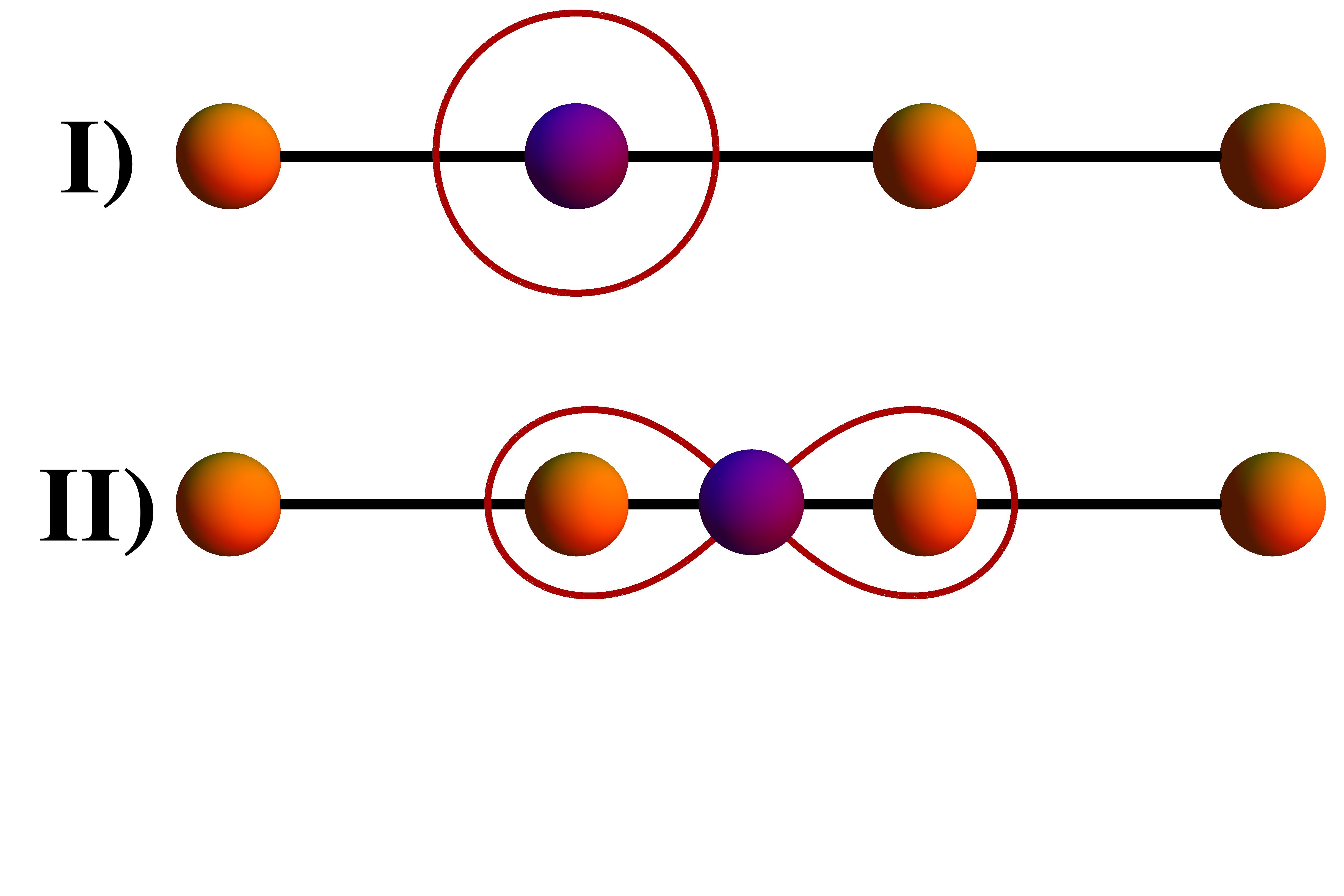
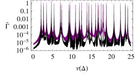
(c)                   (d)

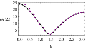
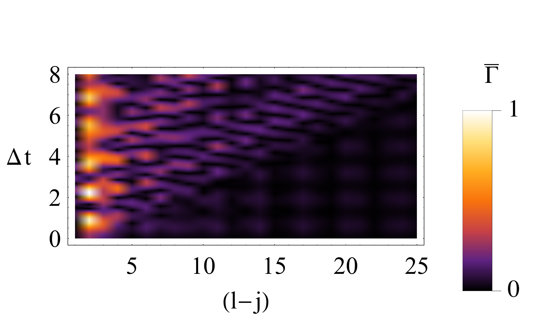
Figure 1: (a) Sketch of a probe overlapping with either one or two lattice sites of a 1-D chain. Measurements in both of the positions are required to perform momentum resolved spectroscopy. (b) Transition probabilities corresponding to the two probe positions, displayed in black and purple, respectively. (c) Reconstructed spectrum. The purple dots are the frequencies extracted from the transition probabilities data, while the black ones are the exact values. Here the source of error is given by the finite sampling in the probe frequency $\nu$. An additional random $2\%$ error has been added to the ratios of the peaks, and $g^{\prime}/g$ has been estimated by summing over them. The agreement is very good, although two points are missing in the dispersion relation. The corresponding frequency is clearly visible in the transition probability, but the errors hinders the estimation of the proper momentum. (d) Quantum correlation function with a clear light-cone structure emerging while it spreads across the lattice. All the plots are drawn for $J/\Delta=5$, $\alpha=0.3$, and $N_{s}=51$. Everywhere, $\Delta$ is the energy and inverse time unit.

III.2 Bose-Hubbard: Superfluid 2D

III.2.1 Bosonic environment and mean field theory

Before moving to the second application of our protocol, we first show, in general terms, how the momentum resolved protocol can be applied in the experimentally relevant case of an interacting gas of cold Bosons. The starting point is to consider that also the probe will interact with the Bose gas via a density-density interaction, which can be described with the usual assumption of a contact potential. Denoting by $\hat{\Phi}(\mathbf{x})$ the many-body field operator, we can write

$$\hat{H}_{int}=\sum_{\bar{n},\bar{m}}\int\mathrm{d}\mathbf{x}\;\psi_{\bar{m}}^{*}(\mathbf{x})\psi_{\bar{n}}(\mathbf{x})\mathinner{|{\bar{m}}\rangle}\mathinner{\langle{\bar{n}}|}\otimes\hat{\Phi}^{\dagger}(\mathbf{x})\hat{\Phi}(\mathbf{x}).$$ (17)

Loosely speaking, with such a probe-system interaction, the probe transition probability will show a resonance every time the energy difference between its levels matches the energy difference between the modes of the many body system (provided the transition is allowed, thanks to a non-vanishing overlapping integral).

By adopting a mean-field description for the lattice many-body system, the field operator can be written as $\hat{\Phi}(\mathbf{x})=\Phi_{0}(\mathbf{x})+\hat{\delta\Phi}(\mathbf{x})$, with $\hat{\delta\Phi}(\mathbf{x})$ describing linear fluctuations around the mean-field value $\Phi_{0}(\mathbf{x})$. Given the lattice structure of the many-body system, we can expand $\delta\Phi(\mathbf{x})=\sum_{\mathbf{k}}w_{\mathbf{k}}(\mathbf{x})\hat{b}_{\mathbf{k}}$, in which $w_{\mathbf{k}}(\mathbf{x})$ are lattice Bloch functions. Neglecting contributions that are quadratic in the fluctuations, the interaction Hamiltonian reads

$$\begin{split}\hat{H}_{int}&=\sum_{\bar{n},\bar{m}}\int\mathrm{d}\mathbf{x}\;\psi_{\bar{m}}^{*}(\mathbf{x})\psi_{\bar{n}}(\mathbf{x})\mathinner{|{\bar{m}}\rangle}\mathinner{\langle{\bar{n}}|}\otimes\\ &\Bigl{\{}\Phi_{0}^{2}+\Phi_{0}\sum_{\mathbf{k}}\left[w_{\mathbf{k}}(\mathbf{x})^{*}\hat{b}_{\mathbf{k}}^{\dagger}+w_{\mathbf{k}}(\mathbf{x})\hat{b}_{\mathbf{k}}\right]\Bigr{\}}.\end{split}$$ (18)

Using the same preparation and measurement procedures discussed in general terms in Sec. II, the rescaled transition rate analogous to that in Eq. (4) reads

$$\Gamma_{\bar{g}\rightarrow\bar{e}}(\nu,t)=g^{2}\Bigl{\{}\Gamma_{0}(\nu,t)+\sum_{k}\Gamma^{-}_{\mathbf{k}}(\nu,t)+\Gamma^{+}_{\mathbf{k}}(\nu,t)\Bigr{\}}\,,$$ (19)

where

$$\Gamma_{0}(\nu,t) =|\gamma_{0}|^{2}\Phi_{0}^{4}\operatorname{sinc}(\nu t),$$ (20)

$$\Gamma^{-}_{\mathbf{k}}(\nu,t) =\Phi_{0}^{2}|J_{0}\gamma_{\mathbf{k}}|^{2}\operatorname{sinc}^{2}\left[\frac{(\nu+\omega_{\mathbf{k}})t}{2}\right](1+n(\omega_{\mathbf{k}})),$$ (21)

$$\Gamma^{+}_{\mathbf{k}}(\nu,t) =\Phi_{0}^{2}|J_{0}\gamma_{\mathbf{k}}|^{2}\operatorname{sinc}^{2}\left[\frac{(\nu-\omega_{\mathbf{k}})t}{2}\right]n(\omega_{\mathbf{k}}).$$ (22)

with $\gamma_{0}=\int\mathrm{d}\mathbf{x}\;\psi_{\bar{e}}^{*}(\mathbf{x})\psi_{\bar{g}}(\mathbf{x})$. For large enough measuring times, resonant peaks appear in the $\nu$-dependent transition rates, whose amplitudes read $A_{\mathbf{k}}^{2}=d_{\mathbf{k}}|J_{\mathbf{0}}\gamma_{k}|^{2}n_{\mathbf{k}}$, if $\nu>0$.

By repeating the measurement with the probe in different positions, as described in Sec. II, the analogous of Eq. (5) can be obtained, from which the momentum resolved spectrum can be finally extracted, as discussed in detail below for the case of a 2D Bose-Hubbard model.

III.2.2 2D Superfluid

Let us now present the second application of our protocol. To this end, we consider a gas of cold bosonic atoms in the lowest energy band of a 2D optical potential. This system is very well described by the Bose-Hubbard model hubbard ; hubbard2 ; kanamori ; jaksch1 :

$$\hat{H}=-J\sum_{\langle l,j\rangle}\hat{c}^{\dagger}_{l}\hat{c}_{j}+\frac{U}{2}\sum_{j}\hat{n}_{j}(\hat{n}_{j}-1)-\mu\sum_{j}\hat{n}_{j}.$$ (23)

In the limit $J\gg U$, the system is in the superfluid phase, with a low-energy spectrum due to phononic excitations above a uniform Bose-Einstein condensate oosten1 . These excitations have been successfully resolved in energy using techniques such as magnetic gradients bloch3 and lattice depth modulation OPL . Furthermore, a full momentum-resolved spectroscopy has been performed using two-photon Bragg spectroscopy in BRAGG ; BRAGG2 . Although quite successful, such methods strongly interfere with the dynamics of the gas and are therefore very invasive. We apply our quantum probe protocols in this case, by assuming the probe immersed in the lattice to be an atomic quantum dot trapped in a 3D harmonic potential, with energy states $\psi_{\bar{n}}(\mathbf{x})=\psi_{n_{x}}^{(\nu_{x})}(x)\psi_{n_{y}}^{(\nu_{y})}(y)\psi_{n_{z}}^{(\nu)}(z)$. As shown in Ref. jaksch2 , the density-density interaction typical of cold atoms, when applied to the case of a superfluid/BEC in the mean-field approach, gives rise to a linear coupling of the impurity to density fluctuations in the many-body system.

To start the reconstruction procedure, we evaluate the transition probability between impurity states along the direction orthogonal to the lattice, say, e.g., the $z$ axis, $\tilde{\Gamma}_{\bar{0}\rightarrow(0,0,n_{z})}$ as a function of the probe trapping frequency in that direction, $\nu_{z}$. As a matter of fact, $\tilde{\Gamma}_{\bar{0}\rightarrow(0,0,n_{z})}$ depends on $\nu_{z}$ as well as on the overlap between the lattice Wannier states and the unperturbed eigenfunctions of the impurity. For the first measurement, we find that the transition rate is given by exactly the same expression reported in Eq. (4), but with the prefactor now given by

$$\begin{split}J_{0}\gamma_{k}=\int dx\,\psi_{n_{x}=0}^{2}(x)W_{0}^{2}(x)\int dy\,\psi_{n_{y}=0}^{2}(y)W_{0}^{2}(y)(-1)^{n_{z}}\sqrt{{m}}\frac{\gamma_{n_{z}}^{1/2}\gamma_{0}^{1/2}}{\pi}\sqrt{\nu_{z}}\beta_{\mathbf{k}},\end{split}$$ (24)

(a)

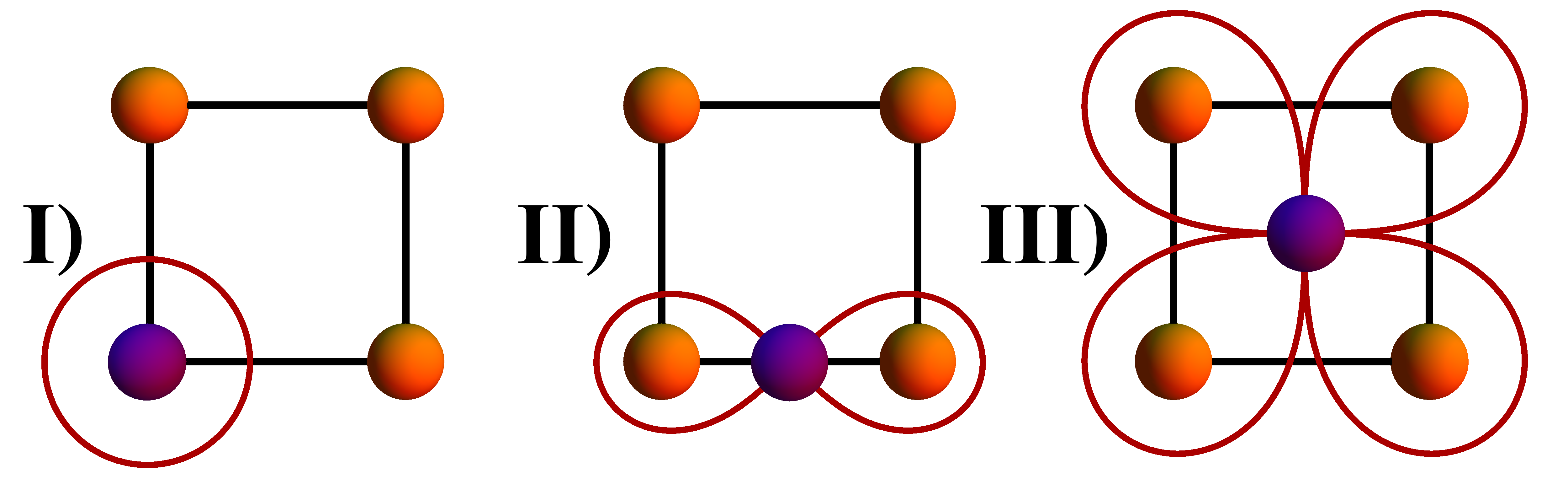
(b)                 (c)

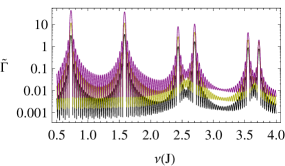
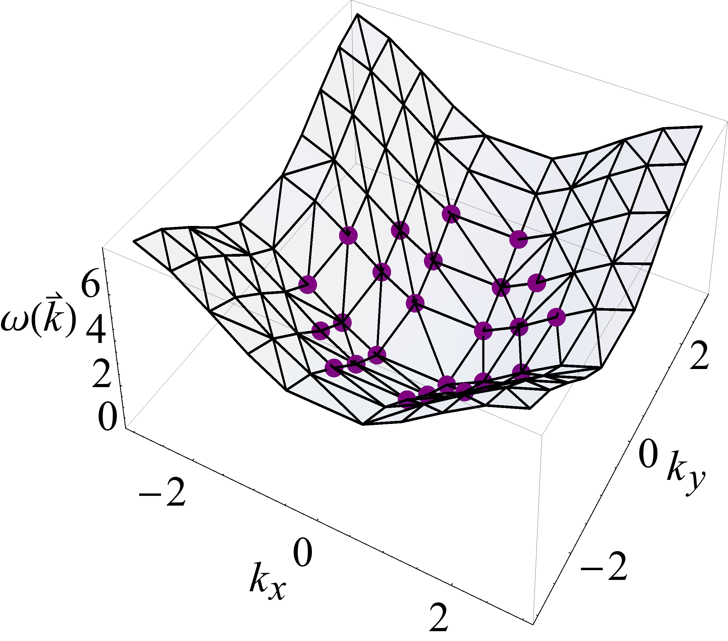
(d)

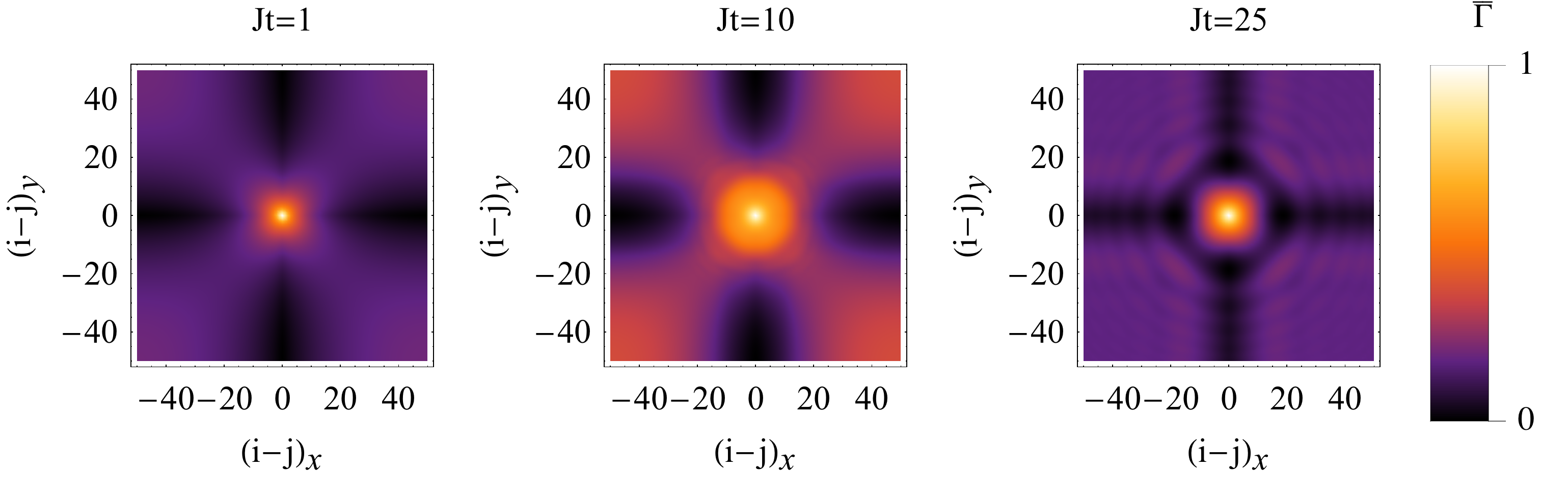
Figure 2: (a) Sketch of the probe-positions in the three stages of the protocol. (b) Semi-log plot of the low-energy transition probabilities $\tilde{\Gamma}^{(\mathrm{I},\mathrm{II},\mathrm{III})}$, rescaled by $|\frac{J_{i}}{J_{0}}|^{2}$, for the three cases shown in (a), drawn in black, yellow and purple, respectively for a lattice of $N_{s}=121$ sites. (c) Reconstructed dispersion relation (purple dots). (d) The correlation function defined in Eq. 26 for a square lattice of $N_{s}=121^{2}$ sites, displayed at three different times. In each plot, the value of the correlation function has been scaled to its maximum, $J$ has been taken as energy and inverse time units, with $U=0.1J$.

As depicted in Fig. 2, and as discussed briefly in general terms above, the reconstruction of the single particle excitation spectrum for a 2D lattice system requires two further measurements, with the probe placed in different positions. Thus, the overall protocol develops in three subsequent steps with the probe placed as in in Fig. 2 (a). I) , II) and III), during which the rates $\Gamma^{\mathrm{I}},\Gamma^{\mathrm{II}}$ and $\Gamma^{\mathrm{III}}$ are extracted.

In a realistic experimental realization the in-plane trapping frequencies, $\nu_{x}$ and $\nu_{y}$, can be modified in order to achieve a suitable wave-function overlap with the nearest neighboring sites, as necessary for the protocol. The information obtained by using these three steps allows for the reconstruction of the full dispersion relation $\omega(\mathbf{k})$. Indeed, by taking the ratios of the second and third transition rates with respect to the first one at each resonant peak, one obtains two relations that can be inverted to extract the two components of the momentum vector $\mathbf{k}=(k_{x},k_{y})$ associated to the selected peak frequency. In our case, we have (see Appendix A for the details)

$$\begin{cases}\frac{\tilde{\Gamma}^{\mathrm{II}}}{\tilde{\Gamma}^{\mathrm{I}}}=2|\frac{J_{1}}{J_{0}}|^{2}\left[\cos^{2}(\frac{k_{x}a}{2})+\cos^{2}(\frac{k_{y}a}{2})\right],\\ \frac{\tilde{\Gamma}^{\mathrm{III}}}{\tilde{\Gamma}^{\mathrm{I}}}=16|\frac{J_{2}}{J_{0}}|^{2}\,\cos^{2}(\frac{k_{x}a}{2})\cos^{2}(\frac{k_{y}a}{2}).\end{cases}$$ (25)

These relations are easily numerically inverted, so that a vector $\mathbf{k}$ is associated to each peak frequency $\omega$ found in the transition rates, with the result reported in Fig. 2.

Finally, for measuring the correlation function, one needs to use two entangled probes, located at sites $l$ and $j$. Following the line of the derivation given above, one obtains the collective decay rate $\overline{\Gamma}$ analogous to that of Eq. (12). For this system we show in detail in Appendix B that the following expression holds:

$$\begin{split}\overline{\Gamma}&=\frac{\bar{g}^{2}}{2}\int_{0}^{t}dt_{1}\int_{0}^{t}dt_{2}\langle\hat{n}_{l}(t_{1})\hat{n}_{j}(t_{2})+\\ &+\hat{n}_{j}(t_{1})\hat{n}_{l}(t_{2})\rangle e^{i\nu(t_{1}-t_{2})},\end{split}$$ (26)

where $\bar{g}$ is a new coupling constant containing the overlap integral. Due to the density-density interaction of the impurity with the boson gas, thus, the function $\overline{\Gamma}$ contains information about the density-density correlation function, whose behaviour can be extracted from the measured values of the transition rates, as reported in Fig. 2.

Both the one- and two-probe protocols are in principle feasible for a 2D superfluid with current technology exp1 ; exp2 ; ott ; osp . In particular, it has been proven that the control of the position of an impurity in an optical lattice can be achieved in different ways. For example using species-selective or spin-selective optical lattice, by changing the polarization angle of the laser beams generating the lattice it is possible to obtain two spin dependent potentials that split in opposite direction cohetransport . Efficient control over a single spin at a specific site of an optical lattice has been achieved recently, with the further benefit of leaving the atom in the vibrational ground state, that is the initial state of our probe singlespin . Detecting the locations of such impurities is nowadays in the grasp of the experimentalists micro1 ; micro2 as well as measuring the populations of excited vibrational states motmeas1 ; motmeas2 .

IV Conclusions

We have demonstrated how global properties of a certain class of many-body systems can be extracted by means of controllable quantum probes. Our approach is rather general, being only based on the assumptions of full control of the probe position and of its interaction with the many-body system. Within such framework, we have demonstrated that it is possible to obtain the single particle excitation spectrum of the system and perform momentum-resolved spectroscopy via energy-resolved measurements on a single quantum probe. Moreover, the spatial profile of the unperturbed Bloch functions can be reconstructed. By exploiting entangled probes that locally alter the equilibrium configuration of the many-body system, it is possible to monitor the spreading of correlations across the latter.

Our description can be applied to diverse systems, and we illustrated the probing procedures for 1) a 1D long range fermionic model, and 2) an interacting boson gas in a 2D lattice. In the second case, in particular, we have exploited the advanced state of the art of the cold atoms field to provide a more detailed and experimentally feasible description. Our proposal exemplifies the essence of the quantum probing approach, wherein some of the typical complexity of a many-body system can be imprinted onto the open dynamics of a smaller system, and thereby locally extracted in a much less invasive way.

The authors would like to thank Dr. Elmar Haller and Prof. Andrew Daley for useful discussions. This work has been supported by the Horizon 2020 EU collaborative project QuProCS (Grant Agreement 641277).

Appendix A Single Probe - Transition probability

In this Appendix, we sketch the perturbative approach leading to the Fermi-Golden-Rule-like equation used to describe the momentum resolved spectroscopy protocol. In general terms, the probability for a ground to excited state transition, due to the interaction with the many-body environment can be written as

$$\begin{split}\Gamma_{\bar{g}\rightarrow\bar{e}}(t)=\mathrm{Tr}_{MB}\mathinner{\langle{\bar{e}}|}\rho(t)\mathinner{|{\bar{e}}\rangle}=\mathrm{Tr}_{MB}\mathinner{\langle{\bar{e}}|}\hat{U}(t)\rho(0)\hat{U}^{\dagger}(t)\mathinner{|{\bar{e}}\rangle},\end{split}$$ (27)

where $\hat{U}(t)$ is the time evolution operator in the interaction picture. With the assumption of weak coupling we can resort to an expansion in powers of $g$, so that $\hat{U}(t)=1+g\hat{U}_{1}(t)+g^{2}\hat{U}_{2}(t)+...$ . Truncating up to the first order in $g$ the relevant term is $\hat{U}_{1}(t)=-i\int_{0}^{t}\,\mathrm{d}t_{1}\hat{H}_{int}(t_{1})$, so that the transition probability takes the form

$$\begin{split}\Gamma_{\bar{g}\rightarrow\bar{e}}(t)&\simeq g^{2}\mathrm{Tr}_{MB}\mathinner{\langle{\bar{e}}|}\hat{U}_{1}(t)\rho(0)\hat{U}_{1}^{\dagger}(t)\mathinner{|{\bar{e}}\rangle}+O(g^{4})\\ &=g^{2}\int_{0}^{t}\,\mathrm{d}t_{1}\int_{0}^{t}\,\mathrm{d}t_{2}\\ &\mathrm{Tr}_{MB}\mathinner{\langle{\bar{e}}|}\hat{H}_{int}(t_{1})\rho(0)\hat{H}_{int}(t_{2})\mathinner{|{\bar{e}}\rangle}+O(g^{4}).\end{split}$$ (28)

In a weak coupling regime, this expression works very well as its first correction would be of fourth order in $g$. For the interaction Hamiltonian in Eq. (2) we get

$$\begin{split}\Gamma_{\bar{g}\rightarrow\bar{e}}(t)&\simeq g^{2}\int_{0}^{t}\,\mathrm{d}t_{1}\int_{0}^{t}\,\mathrm{d}t_{2}\\ &\mathrm{Tr}_{MB}\left\{\hat{\Phi}{[\bar{e},\bar{g}]}(t_{1})\rho_{\beta}\hat{\Phi}^{\dagger}{[\bar{g},\bar{e}]}(t_{2})\right\}e^{-i\nu t_{2}}e^{i\nu t_{1}}\\ &=g^{2}\int_{0}^{t}\,\mathrm{d}t_{1}\int_{0}^{t}\,\mathrm{d}t_{2}\langle\hat{\Phi}^{\dagger}{[\bar{g},\bar{e}]}(t_{1})\hat{\Phi}{[\bar{e},\bar{g}]}(t_{2})\rangle\\ &e^{-i\nu(t_{1}-t_{2})}.\end{split}$$ (29)

In order to proceed further, we recall that $\hat{\Phi}{[\bar{m},\bar{n}]}\propto\sum_{\mathbf{k}}\gamma^{\mathbf{k}}_{\bar{m},\bar{n}}\hat{b}_{\mathbf{k}}$, with which it is easy to obtain

$$\begin{split}\Gamma_{\bar{g}\rightarrow\bar{e}}(t)&=g^{2}\int_{0}^{t}\,\mathrm{d}t_{1}\int_{0}^{t}\,\mathrm{d}t_{2}\sum_{\mathbf{k},\mathbf{q}}\gamma^{\mathbf{k}}_{\bar{e},\bar{g}}\gamma^{\mathbf{q}*}_{\bar{e},\bar{g}}\langle\hat{b}^{\dagger}_{\mathbf{k}}b_{\mathbf{q}}\rangle\\ &e^{i(\omega_{\mathbf{k}}-\nu)t_{1}}e^{-i(\omega_{\mathbf{q}}-\nu)t_{2}}\\ &=g^{2}\sum_{\mathbf{k}}|\gamma^{\mathbf{k}}_{\bar{e},\bar{g}}|^{2}n_{\mathbf{k}}|\int_{0}^{t}\,\mathrm{d}t_{1}e^{i(\omega_{\mathbf{k}}-\nu)t_{1}}|^{2}\\ &=g^{2}t^{2}\sum_{\mathbf{k}}|\gamma^{\mathbf{k}}_{\bar{e},\bar{g}}|^{2}n_{\mathbf{k}}\operatorname{sinc}^{2}[\frac{(\nu-\omega_{\mathbf{k}})t}{2}],\end{split}$$ (30)

as reported in Eq. 4. However, to perform full momentum resolved spectroscopy we need to know the geometry of the system we intend to probe. This information is crucial in order to define the positions required for the different measurements required by the protocol and the relations among them, which are embodied in the functions $G_{i}(\mathbf{k})$.

As an example, here we calculate the functions $G_{i}(\mathbf{k})$ for a simple square lattice in 2D. The $\mathbf{k}$-dependent amplitudes are assumed to depend on an overlapping integral that involves the probe unperturbed eigenfunctions and on the Bloch functions of the lattice system $\gamma^{\mathbf{k}}_{\bar{m},\bar{n}}=\int\mathrm{d}\mathbf{x}\;\psi_{\bar{e}}^{*}(\mathbf{x})\psi_{\bar{g}}(\mathbf{x})w_{\mathbf{k}}(\mathbf{x})$. The Bloch functions can, in turn, be expanded in the Wannier basis as $w_{\mathbf{k}}(\mathbf{x})=\sum_{\mathbf{r}}\gamma_{\mathbf{k}}e^{i\mathbf{k}\mathbf{r}}W_{\mathbf{r}}(\mathbf{x})$. In a 2D scenario, measurements in three different positions are required. The optimal basis is represented by the following positions $\left\{a_{0}=(0,0),a_{1}=(1/2,0),a_{2}=(1/2,1/2)\right\}$. In the first measurement the impurity is exactly on top of a lattice site and the locality of the interaction allows us to consider as relevant only the overlapping integral that involves a single Wannier state (the one centered on the site (0,0)). In the two other cases, the nearest neighbours contribute equally to the overlapping integral, giving two further contributions for the second measurement and four in the third one. These assumptions about the localisation of the probe allow to replace the Bloch functions in the three overlapping integrals in the following way

$$\begin{split}w_{\mathbf{k}}(\mathbf{x})&\simeq\begin{cases}\gamma_{\mathbf{k}}W_{(0,0)}(\mathbf{x})\\ \gamma_{\mathbf{k}}(W_{(0,0)}(\mathbf{x})+e^{i\mathbf{k}_{x}}W_{(1,0)}(\mathbf{x}))\\ \gamma_{\mathbf{k}}(W_{(0,0)}(\mathbf{x})+e^{i\mathbf{k}_{y}}W_{(0,1)}(\mathbf{x})+\\ +e^{i\mathbf{k}_{x}}W_{(1,0)}(\mathbf{x})+e^{i\mathbf{k}}W_{(1,1)}(\mathbf{x}))\end{cases}\end{split}$$ (31)

For a perfect and regular lattice, Wannier functions centered on different sites have the same shape. The amplitudes associated to each transition are, then,

$$\begin{cases}|J_{0}\gamma_{\mathbf{k}}!^{2}\\ |J_{1}\gamma_{\mathbf{k}}|^{2}2[1+\cos(k_{x})]\\ |J_{2}\gamma_{\mathbf{k}}|^{2}[16\cos^{2}(\frac{k_{x}a}{2})\cos^{2}(\frac{k_{y}a}{2})]\\ \end{cases}$$ (32)

where $J_{i}=\int\mathrm{d}\mathbf{x}\;\psi_{\bar{e}}^{*}(\mathbf{x}-{\mathbf{a}_{i}})\psi_{\bar{g}}(\mathbf{x}-{\mathbf{a}_{i}})W_{(0,0)}(\mathbf{x})$, with $i=0,1,2$. It is important to mention that each resonant peak depends on all the transitions with equal energy; in other words, it is a sum of the contributions from all the possible transitions with the same energy. This approach takes into account only the degeneracy given by the geometry. Thanks to these considerations, we find

$$\sum_{\mathbf{k}|\nu=\omega_{\mathbf{k}}}G_{i}(\mathbf{k})=\begin{cases}2\cos^{2}(\frac{k_{x}a}{2})+2\cos^{2}(\frac{k_{y}a}{2})\quad i=1\\ 16\cos^{2}(\frac{k_{x}a}{2})\cos^{2}(\frac{k_{y}a}{2})\,\qquad i=2\end{cases}.$$ (33)

In 1D, just two different positions are required, and the optimal choice is given by the probe on top of a lattice site and between two adjacent sites. With this choice it is easy to find under the same assumptions of a local interaction

$$\sum_{k|\nu=\omega_{\mathbf{k}}}G(k)=4\cos^{2}(\frac{ka}{2})$$ (34)

Appendix B Two Probes - Transition probability

In this Appendix, we derive the combined rate given in Eq. (12) that allows to probe spatial quantum correlations. The starting point is to assume that the environment and the two probes interact locally on two different sites

$$\hat{H}_{int}=\sum_{\bar{n},\bar{m}}\mathinner{|{\bar{n}}\rangle}_{A}\mathinner{\langle{\bar{m}}|}_{A}\otimes\hat{\Phi}_{\mathbf{x}_{A}}^{[\bar{m}_{A},\bar{n}_{A}]}+\sum_{\bar{n},\bar{m}}\mathinner{|{\bar{n}}\rangle}_{B}\mathinner{\langle{\bar{m}}|}_{B}\otimes\hat{\Phi}_{\mathbf{x}_{B}}^{[\bar{m}_{B},\bar{n}_{B}]},$$ (35)

where $\hat{\Phi}_{\mathbf{x}_{A}}^{[m,n]}$ and $\hat{\Phi}_{\mathbf{x}_{B}}^{[m,n]}$ are the observables whose correlations we want to study. We consider two entangled probes $\mathinner{|{\Psi}\rangle}=\frac{1}{\sqrt{2}}(\mathinner{|{n_{A},s_{B}}\rangle}+\mathinner{|{m_{A},r_{B}}\rangle})$, so that the total state of the system reads

$$\begin{split}\hat{\rho}_{tot}&=\mathinner{|{\Psi}\rangle}\mathinner{\langle{\Psi}|}\otimes\hat{\rho}\\ &=\frac{1}{2}(\mathinner{|{n_{A},s_{B}}\rangle}\mathinner{\langle{n_{A},s_{B}}|}+\mathinner{|{n_{A},s_{B}}\rangle}\mathinner{\langle{m_{A},r_{B}}|}\\ &+\mathinner{|{m_{A},r_{B}}\rangle}\mathinner{\langle{n_{A},s_{B}}|}+\mathinner{|{m_{A},r_{B}}\rangle}\mathinner{\langle{m_{A},r_{B}}|})\otimes\hat{\rho}.\end{split}$$ (36)

We calculate the transition probability $\Gamma(\mathinner{|{m_{A}s_{B}}\rangle})=\mathinner{\langle{m_{A},s_{B}}|}\hat{\rho}_{tot}(t)\mathinner{|{m_{A},s_{B}}\rangle}$ resorting to an expansion of the time evolution operator to the first order in $g$, as for the single probe case. After a few straightforward steps, we find

$$\begin{split}&\Gamma(\mathinner{|{m_{A}s_{B}}\rangle})\simeq\frac{1}{2}\int_{0}^{t}dt_{1}\int_{0}^{t}dt_{2}\\ &\langle e^{i(\nu_{mA}-\nu_{nA})t_{1}}\hat{\Phi}_{\mathbf{x}_{A}}^{[m_{A},n_{A}]}(t_{1})e^{i(\nu_{nA}-\nu_{mA})t_{2}}\hat{\Phi}_{\mathbf{x}_{A}}^{[n_{A},m_{A}]}(t_{2})\\ &+e^{i(\nu_{sB}-\nu_{rB})t_{1}}\hat{\Phi}_{\mathbf{x}_{B}}^{[s_{B},r_{B}]}(t_{1})e^{i(\nu_{rB}-\nu_{sB})t_{2}}\hat{\Phi}_{x_{B}}^{[r_{B},s_{B}]}(t_{2})\\ &+e^{i(\nu_{mA}-\nu_{nA})t_{1}}\hat{\Phi}_{\mathbf{x}_{A}}^{[m_{A},n_{A}]}(t_{1})e^{i(\nu_{rB}-\nu_{sB})t_{2}}\hat{\Phi}_{\mathbf{x}_{B}}^{[r_{B},s_{B}]}(t_{2})\\ &+e^{i(\nu_{sB}-\nu_{rB})t_{1}}\hat{\Phi}_{\mathbf{x}_{B}}^{[s_{B},r_{B}]}(t_{1})e^{i(\nu_{nA}-\nu_{mA})t_{2}}\hat{\Phi}_{\mathbf{x}_{A}}^{[n_{A},m_{A}]}(t_{2})\rangle\\ \end{split}$$ (37)

Combining the result with the transition probabilities obtained in separate single probe experiments ($\hat{\rho}_{tot}=\mathinner{|{n_{A}}\rangle}\mathinner{\langle{n_{A}}|}\hat{\rho}$ and $\hat{\rho}_{tot}=\mathinner{|{r_{B}}\rangle}\mathinner{\langle{r_{B}}|}\otimes\hat{\rho}$ ) we get Eq. (12)

$$\begin{split}\overline{\Gamma}&=\Gamma(\mathinner{|{m_{A}s_{B}}\rangle})-\frac{1}{2}\Gamma{(\mathinner{|{m_{A}}\rangle})}-\frac{1}{2}\Gamma{(\mathinner{|{s_{B}}\rangle})}\\ &=\frac{g^{2}}{2}\int_{0}^{t}dt_{1}\int_{0}^{t}dt_{2}\\ &\langle\hat{\Phi}_{\mathbf{x}_{A}}^{[m_{A},n_{A}]}(t_{1})\hat{\Phi}_{\mathbf{x}_{B}}^{[r_{B},s_{B}]}(t_{2})e^{i(\nu_{mA}-\nu_{nA})t_{1}}e^{i(\nu_{rB}-\nu_{sB})t_{2}}\\ &+\hat{\Phi}_{\mathbf{x}_{B}}^{[s_{B},r_{B}]}(t_{1})\hat{\Phi}_{\mathbf{x}_{A}}^{[n_{A},m_{A}]}(t_{2})e^{i(\nu_{sB}-\nu_{rB})t_{1}}e^{i(\nu_{nA}-\nu_{mA})t_{2}}\rangle.\end{split}$$ (38)

If the two probes are identical, and choosing $\nu_{mA}-\nu_{nA}=\nu_{sB}-\nu_{rB}=\nu$ in order to simplify the function $\overline{\Gamma}$, we have

$$\begin{split}\overline{\Gamma}&=\frac{g^{2}}{2}\int_{0}^{t}dt_{1}\int_{0}^{t}dt_{2}\langle\hat{\Phi}_{\mathbf{x}_{A}}^{[m_{A},n_{A}]}(t_{1})\hat{\Phi}_{\mathbf{x}_{B}}^{[r_{B},s_{B}]}(t_{2})+\\ &+\hat{\Phi}_{\mathbf{x}_{B}}^{[s_{B},r_{B}]}(t_{1})\hat{\Phi}_{\mathbf{x}_{A}}^{[n_{A},m_{A}]}(t_{2})\rangle e^{\nu(t_{1}-t_{2})}.\end{split}$$ (39)

B.1 Density-density correlation function

In this section, we explicitly derive the expression of $\overline{\Gamma}$ for the case in which the probes and the many-body system interact via a density-density interaction, as that introduced in the discussion of the probing of the superfluid,

$$g\sum_{\bar{n},\bar{m}}\int\mathrm{d}\mathbf{x}\;\psi_{\bar{m}}^{*}(\mathbf{x})\psi_{\bar{n}}(\mathbf{x})\mathinner{|{\bar{m}}\rangle}\mathinner{\langle{\bar{n}}|}\otimes\hat{\Phi}^{\dagger}(\mathbf{x})\hat{\Phi}(\mathbf{x}).$$ (40)

Assuming a probe to be localized in the site $j$, the auxiliary operator is defined as

$$\hat{\Phi}_{\mathbf{x}_{j}}^{[m,n]}=\int\mathrm{d}\mathbf{x}\;\psi_{\bar{m}}^{*}(\mathbf{x}-\mathbf{x}_{j})\psi_{\bar{n}}(\mathbf{x}-\mathbf{x}_{j})\hat{\Phi}^{\dagger}(\mathbf{x})\hat{\Phi}(\mathbf{x}).$$ (41)

Expanding the many-body field operator in terms of Wannier functions,

$$\hat{\Phi}_{\mathbf{x}_{j}}^{[m,n]}=\int\mathrm{d}\mathbf{x}\;\psi_{\bar{m}}^{*}(\mathbf{x}-\mathbf{x}_{j})\psi_{\bar{n}}(\mathbf{x}-\mathbf{x}_{j})W^{*}_{i}(\mathbf{x})W_{l}(\mathbf{x})\hat{c}_{i}^{\dagger}\hat{c}_{l},$$ (42)

we can take advantage of the localisation of the probe, ensuring that the only relevant overlapping integral is that involving the Wannier functions of the site under the probe. Therefore we get

$$\hat{\Phi}_{\mathbf{x}_{j}}^{[m,n]}\simeq\gamma_{\bar{n}\bar{m}}\hat{c}_{j}^{\dagger}\hat{c}_{j}=\gamma_{\bar{n}\bar{m}}\hat{n}_{j},$$ (43)

with $\gamma_{\bar{n}\bar{m}}=\int\mathrm{d}\mathbf{x}\;\psi_{\bar{m}}^{*}(\mathbf{x}-\mathbf{x}_{j})\psi_{\bar{n}}(\mathbf{x}-\mathbf{x}_{j})|W_{j}(\mathbf{x})|^{2}$, and with $\hat{n}_{j}$ being the density operator for site $j$. By inserting this result into the general form of Eq. (39), we obtain Eq. (26)

$$\overline{\Gamma}=\frac{\bar{g}^{2}}{2}\int_{0}^{t}dt_{1}\int_{0}^{t}dt_{2}\langle\hat{n}_{l}(t_{1})\hat{n}_{j}(t_{2})+\hat{n}_{j}(t_{1})\hat{n}_{l}(t_{2})\rangle e^{i\nu(t_{1}-t_{2})},$$ (44)

where $\bar{g}=g\gamma_{\bar{n}\bar{m}}$.

References

- [1] I. Bloch, J. Dalibard, and W. Zwerger, Rev. Mod. Phys. 80, 885 (2008).
- [2] M. A. Cazalilla, R. Citro, T. Giamarchi, E. Orignac, and M. Rigol, Rev. Mod. Phys. 83, 1405 (2011).
- [3] I. Bloch, J. Dalibard, and S. Nascimbène, Nature Physics 8, 267-276 (2012).
- [4] O. Mandel, M. Greiner, A. Widera, T. Rom, T. W. Hänsch, and I. Bloch, Nature 425, 937 (2003).
- [5] M. Greiner, O. Mandel, T. W. Hänsch, and I. Bloch, Nature 419, 51 (2002).
- [6] D. Jaksch and P. Zoller, Annals of Physics Volume 315, Issue 1, Pages 52–79, (2005).
- [7] J. Catani, G. Barontini, G. Lamporesi, F. Rabatti, G. Thalhammer, F. Minardi, S. Stringari, and M. Inguscio, Phys. Rev. Lett. 103, 140401 (2009).
- [8] M. Cetina, M. Jag, R. S. Lous, I. Fritsche, J. T. M. Walraven, R. Grimm, J. Levinsen, M. M. Parish, R. Schmidt, M. Knap, and E. Demler, Science Vol. 354, Issue 6308, pp. 96-99, (2016).
- [9] C. Weitenberg, M. Endres, J. F. Sherson, M. Cheneau, P. Schauß, T. Fukuhara, I. Bloch, and S. Kuhr, Nature 471, 319–324 (2016).
- [10] K. Mayer, A. Rodriguez, and A. Buchleitner, Phys. Rev. A 90, 023629 (2014).
- [11] K. Mayer, A. Rodriguez, and A. Buchleitner, Phys. Rev. A 91, 053633 (2015).
- [12] T. H. Johnson, S. R. Clark, M. Bruderer, and D. Jaksch, Phys. Rev. A 84, 023617 (2011).
- [13] M. Bruderer and D. Jaksch, New J. Phys. 8 87, (2006).
- [14] A. Kantian, U. Schollwãck, and T. Giamarchi, Phys. Rev. Lett. 115, 165301 (2015).
- [15] T. J. Elliot, and T. H. Johnson, Phys. Rev. A 93, 043612 (2016).
- [16] M. T. Mitchison, T. H. Johnson, and D. Jaksch, Phys. Rev. A 94, 063618 (2016).
- [17] T. H. Johnson, F. Cosco, M. T. Mitchison, D. Jaksch, and S. R. Clark, Phys. Rev. A 93, 053619 (2016).
- [18] D. Hangleiter, M. T. Mitchison, T. H. Johnson, M. Bruderer, M. B. Plenio, and D. Jaksch, Phys. Rev. A 91, 013611 (2015).
- [19] A. Recati, P. O. Fedichev, W. Zwerger, J. von Delft, and P. Zoller, Phys. Rev. Lett. 94, 040404 (2005).
- [20] A. Sindona, J. Goold, N. Lo Gullo, S. Lorenzo, and F. Plastina, Phys. Rev. Lett. 111, 165303 (2013).
- [21] P. O. Fedichev and U. R. Fischer, Phys. Rev. Lett. 91, 240407 (2003).
- [22] M. Schirò and A. Mitra, Phys. Rev. Lett. 112, 246401 (2014).
- [23] M. Knap, A. Shashi, Y. Nishida, A. Imambekov, D. A. Abanin, and E. Demler, Phys. Rev. X 2, 041020 (2012).
- [24] P. Haikka, S. McEndoo, G. De Chiara, G. M. Palma, and S. Maniscalco, Phys. Rev. A 84, 031602 (2011).
- [25] P. Haikka, S. McEndoo, and S. Maniscalco, Phys. Rev. A 87, 012127 (2013).
- [26] D. Tamascelli, C. Benedetti, S. Olivares, and M. G. A. Paris , Phys. Rev. A 94, 042129 (2016).
- [27] A. Zwick, G. A. Alvarez, and G. Kurizki, Phys. Rev. A 94, 042122 (2016).
- [28] M. Borrelli, P. Haikka, G. De Chiara, and S. Maniscalco, Phys. Rev. A 88, 010101(R) (2013).
- [29] M. Borrelli, and S. Maniscalco, Int. J. Quantum Inform. 12, 1461006 (2014).
- [30] P. Haikka, J. Goold, S. McEndoo, F. Plastina, and S. Maniscalco, Phys. Rev. A 85, 060101(R) (2012).
- [31] G. Francica, T. J. G. Apollaro, N. Lo Gullo, F. Plastina, Phys. Rev. B 94, 245103 (2016).
- [32] J. Nokkala, F. Galve, R. Zambrini, S. Maniscalco, and J. Piilo, Scientific Reports 6, 26861 (2016).
- [33] S. Cialdi, C. Porto, D. Cipriani, S. Olivares, and M. G. A. Paris, Phys. Rev. A 93, 043805 (2016).
- [34] M. A. Rossi, T. Giani, and M. G. A. Paris, Phys. Rev. D 94, 024014 (2016).
- [35] V. Giovannetti, S. Lloyd, and L. Maccone, Phys. Rev. Lett. 96, 010401 (2006).
- [36] M. A. C. Rossi and M. G. A. Paris, Phys. Rev. A 92, 010302(R) (2015).
- [37] A. W. Chin, S. F. Huelga, and M. B. Plenio, Phys. Rev. Lett. 109, 233601 (2012).
- [38] S. Mancini and P. Tombesi, Europhys. Lett. 61, 8 (2003)
- [39] W.-M. Zhang, P.-Y. Lo, H.-N. Xiong, M. W.-Y. Tu, and F. Nori, Phys. Rev. Lett. 109, 170402 (2012).
- [40] E. H. Lieb and D. W. Robinson, Commun.Math. Phys. 28, 251 (1972).
- [41] P. Hauke and L. Tagliacozzo, Phys. Rev. Lett. 111, 207202 (2013).
- [42] A. S. Buyskikh, M. Fagotti, J. Schachenmayer, F. Essler, and A. J. Daley, Phys. Rev. A 93, 053620 (2016).
- [43] F. Pientka, L. I. Glazman and F Von Oppen, Phys. Rev. B 88, 155420 (2013).
- [44] F. Pientka, L. I. Glazman and F Von Oppen, Phys. Rev. B 89, 180505 (2014).
- [45] D. Porras and J. I. Cirac, Phys. Rev. Lett. 92, 207901 (2004).
- [46] J. Simon, W. S. Bakr, R. Ma, M. Eric Tai, P. M. Preiss, and M. Greiner, Nature 472, 307–312 (2011).
- [47] F. Meinert, M. J. Mark, E. Kirilov, K. Lauber, P. Weinmann, M. Gröbner, A. J. Daley, and H.-C. Nägerl, Science 344, (6189), 1259-1262 (2014).
- [48] D. Vodola, L. Lepori, E. Ercolessi, A. V. Gorshkov, and G. Pupillo, Phys. Rev. Lett. 113, 156402 (2014).
- [49] D. Vodola, L. Lepori, E. Ercolessi, and G. Pupillo, New J. Phys 18, 015001 (2015).
- [50] J. Hubbard, Proc. R. Soc. London A 276, 238 (1963).
- [51] J. Hubbard, Proc. R. Soc. London A 281, 401 (1964).
- [52] J. Kanamori, Prog. Theor. Phys. 20, 275 (1963).
- [53] D. Jaksch, C. Bruder, J. I. Cirac, C. W. Gardiner, and P. Zoller, Phys. Rev. Lett. 81, 3108 (1998).
- [54] D. van Oosten, P. van der Straten, and H. T. C. Stoof, Phys. Rev. A 63, 053601 (2001).
- [55] M. Greiner, O. Mandel, T. Esslinger, T. W. Hänsch, and I. Bloch, Nature 415, 39 (2002).
- [56] C. Schori, T. Stöferle, H. Moritz, M. Köhl, and T. Esslinger, Phys. Rev. Lett 93, 240402 (2004).
- [57] X. Du, S. Wan, E. Yesilada, C Ryu, D. J. Heinzen, Z. Liang, and B. Wu, New J. Physics 12, 083025 (2010).
- [58] P. T. Ernst, S. Götze, J. S. Krauser, K. Pyka, D.-S. Lühmann, D. Pfannkuche, and K. Sengstock, Nature Physics 6, 56 - 61 (2010).
- [59] D. McKay, and B. DeMarco, New J. Phys 12, 055013 (2010).
- [60] H. Ott, E. de Mirandes, F. Ferlaino, G. Roati, G. Modugno, and M. Inguscio, Phys. Rev. Lett. 92, 160601 (2004).
- [61] S. Ospelkaus, C. Ospelkaus, O. Wille, M. Succo, P. Ernst, K. Sengstock, and K. Bongs, Phys. Rev. Lett. 96, 180403 (2006).
- [62] O. Mandel, M. Greiner, A. Widera, T. Rom, T. W. Hänsch, and I. Bloch Phys. Rev. Lett. 91, 010407 (2003).
- [63] W. S. Bakr, J. I. Gillen, A. Peng, S. Fölling, and M. Greiner, Nature 462, 74-77 (2009).
- [64] J. F. Sherson, C. Weitenberg, M. Endres, M. Cheneau, I. Bloch, and S. Kuhr, Nature 467, 68–72 (2010).
- [65] N. Belmechri, L. Förster, W. Alt, A. Widera, D. Meschede, and A. Alberti, J. Phys. B: At. Mol. Opt. Phys. 46, 104006 (2013).
- [66] D. Leibfried, D. M. Meekhof, B. E. King, C. Monroe, W. M. Itano, and D. J. Wineland, Phys. Rev. Lett. 77, 4281 (1996).