THE GRISM LENS-AMPLIFIED SURVEY FROM SPACE (GLASS). V. Extent and spatial distribution of star formation in $z\approx 0.5$ cluster galaxies

Abstract

We present the first study of the spatial distribution of star formation in $z\sim 0.5$ cluster galaxies. The analysis is based on data taken with the Wide Field Camera 3 as part of the Grism Lens-Amplified Survey from Space (GLASS). We illustrate the methodology by focusing on two clusters (MACS0717.5+3745 and MACS1423.8+2404) with different morphologies (one relaxed and one merging) and use foreground and background galaxies as field control sample. The cluster+field sample consists of 42 galaxies with stellar masses in the range 10⁸-10¹¹ M_⊙, and star formation rates in the range 1-20 M${}_{\odot}\,yr^{-1}$. Both in clusters and in the field, H$\alpha$ is more extended than the rest-frame UV continuum in 60% of the cases, consistent with diffuse star formation and inside out growth. In $\sim$ 20% of the cases, the H$\alpha$  emission appears more extended in cluster galaxies than in the field, pointing perhaps to ionized gas being stripped and/or star formation being enhanced at large radii. The peak of the H$\alpha$ emission and that of the continuum are offset by less than 1 kpc. We investigate trends with the hot gas density as traced by the X-ray emission, and with the surface mass density as inferred from gravitational lens models and find no conclusive results. The diversity of morphologies and sizes observed in H$\alpha$ illustrates the complexity of the environmental process that regulate star formation. Upcoming analysis of the full GLASS dataset will increase our sample size by almost an order of magnitude, verifying and strengthening the inference from this initial dataset.

1. Introduction

Over the past decade, observations have shown that the star formation activity in galaxies has strongly declined since $z\sim 2$ (see, e.g., Hopkins & Beacom, 2006; Madau & Dickinson, 2014), with a large number of star-forming galaxies evolving into passive galaxies at later times, and the star formation rate at fixed mass progressively decreasing (Bell et al., 2004, 2007; Noeske et al., 2007; Daddi et al., 2007; Karim et al., 2011). The evolution of the star formation activity is coupled to the evolution of galaxy morphologies (Poggianti et al., 2009), with a significant fraction of today’s early-type galaxies having evolved from late types at relatively recent epochs. Even though transformations occur both in galaxy clusters (Dressler et al., 1997; Fasano et al., 2000) and in the field (Oesch et al., 2010; Capak et al., 2007), the strength of the decline has been found to depend on environment: galaxies in clusters experience a stronger evolution in star formation activity compared to galaxies in the field (e.g., Poggianti et al., 2006; Cooper et al., 2006; Guglielmo et al., 2015).

Central for our progress in understanding galaxy evolution is identifying the cause of the decline of star formation and of the emergence of the different galaxy types. The mass of galaxies and the environment where they reside are generally believed to play a role for quenching the star formation (e.g., Peng et al., 2010), but the specific physical mechanisms involved remain obscure. There is no consensus on whether there is one process that dominates quenching across all environments or whether some processes play a larger role in driving galaxy evolution in dense environments than they do in the field (Butcher & Oemler, 1984; Poggianti et al., 1999; Dressler et al., 1999; Treu et al., 2003; Dressler et al., 2013).

Each of the processes that have been proposed to quench star formation in galaxies should leave a different signature on the spatial distribution of the star formation activity within the galaxy. For example, ram-pressure stripping from the disk due to the interaction between the galaxy interstellar medium (ISM) and the intergalactic medium (IGM, Gunn & Gott, 1972) is expected to partially or completely remove the ISM, leaving a recognizable pattern of star formation with truncated H$\alpha$ disks smaller than the undisturbed stellar disk (e.g., Yagi et al., 2015). Strangulation, which is the removal of the hot gas halo surrounding the galaxy either via ram-pressure or via tidal stripping by the halo potential (Larson, Tinsley & Caldwell, 1980; Balogh, Navarro & Morris, 2000), should deprive the galaxy of its gas reservoir, and leave the existing interstellar medium in the disk to be consumed by star formation. Strong tidal interactions and mergers, tidal effects of the cluster as a whole and harassment, that is the cumulative effect of several weak and fast tidal encounters (Moore et al., 1996), thermal evaporation (Cowie & Songaila, 1977) and turbulent/viscous stripping (Nulsen, 1982) can also deplete the gas in a non homogeneous way.

In order to address how star formation is suppressed in the different regions of the galaxy, a key ingredient is the spatial distributions of both the past star formation, as traced by the existing stellar population, and of the instantaneous star formation. The latter can be traced by the H$\alpha$ line emission as it scales with the quantity of ionizing photons produced by hot young stars (Kennicutt, 1998).

In the local universe, a few studies have focused on the analysis of H$\alpha$ spatial distribution of a limited number of systems in clusters (e.g. Merluzzi et al., 2013; Fumagalli et al., 2014), detecting debris of material that appear to be stripped from the main body of the galaxy, and whose morphology is suggestive of gas-only removal mechanisms, such as ram pressure stripping.

However, our current understanding is that much of the activity in cluster galaxies happens beyond the local universe at $z=0-1$ and it is therefore essential to gather information in this redshift range. A number of H$\alpha$ surveys up to $z\sim$1 have been undertaken in the field using narrow-band imaging (e.g., Sobral et al., 2013) and with WFC3 grism observations (e.g., Atek et al., 2010; Straughn et al., 2011). In clusters, narrow-band H$\alpha$  studies are available for just a few systems at $z=0.3-1$ (Kodama et al., 2004; Finn et al., 2005; Koyama et al., 2011) and a few other higher-$z$ overdense regions (Kurk et al. 2004a; Kurk et al. 2004b; Geach et al. 2008; Hatch et al. 2011; Koyama et al. 2013). These ground-based studies provide integrated H$\alpha$ fluxes, and no spatial information.

Recently, spatially resolved star formation maps at $z\sim 1$ have been obtained for field galaxies using both the ACS I band and the G141 grism on the Wide Field Camera 3 (WFC3) on board the Hubble Space Telescope (HST) as part of the 3D-HST Survey (van Dokkum et al. 2011; Brammer et al. 2012; Schmidt et al. 2013; Momcheva et al. in prep). Nelson et al. (2012, 2013) mapped the H$\alpha$ and stellar continuum with high resolution for $\sim$ 60 galaxies and showed that star formation broadly follows the rest-frame optical light, but is slightly more extended. By stacking the H$\alpha$ emission, they measured structural parameters of stellar continuum emission and star formation, finding that star formation occurred in approximately exponential distributions. They concluded that star formation at $z\sim$1 generally occurred in disks.

Wuyts et al. (2013) expanded the sample analyzed by Nelson et al. (2012, 2013) and characterized the resolved stellar populations of $\sim$500 massive star-forming galaxies, with multi-wavelength broad-band imaging from CANDELS (Wuyts et al., 2012) and H$\alpha$ surface brightness profiles. They found the H$\alpha$ morphologies to resemble more closely those observed in the ACS I band than in the WFC3 H band, especially for the larger systems. They also found that the rate of ongoing star formation per unit area tracks the amount of stellar mass assembled over the same area. Off-center clumps are characterized by enhanced H$\alpha$ equivalent widths, bluer broad-band colors and correspondingly higher specific star formation rates (SFRs) than the underlying disk, implying they are a star formation phenomenon.

More recently, Nelson et al. (2015), exploiting a much larger sample, studied the behavior of the H$\alpha$ profiles above and below the main sequence and showed that star formation is enhanced at all radii above the main sequence, and suppressed at all radii below the main sequence.

In this paper we present a pilot study characterizing the spatial distribution of the H$\alpha$ emission in cluster galaxies beyond the local universe based on WFC3-IR data drawn from the Grism Lens-Amplified Survey from Space (GLASS; GO-13459; PI: Treu, Schmidt et al. 2014; Treu et al. 2015). The GLASS G102 data yield spatially resolved H$\alpha$ fluxes for all star-forming galaxies in the core ($<1$ Mpc) of 10 clusters at $z=0.31-0.69$, with an order of magnitude improvement in sensitivity compared to previous studies (Sobral et al., 2013). Each cluster is observed at two different position angles. These two orientations allow us to mitigate the impact of contamination from overlapping spectra, and reliably measure for the first time the relative position of the H$\alpha$ emission with respect to the continuum.

We illustrate the methodology and first results of this approach by analyzing two of the ten clusters in the GLASS sample. Among the first clusters that have been observed by GLASS we selected MACS0717.5+3745 (hereafter MACS0717) and MACS1423.8+2404 (hereafter MACS1423) based on the following criteria. First, we required similar redshift, so as to minimize evolutionary effects and differences in the sensitivity/selection function ($z=0.55$). Second, we selected them to be in very different dynamical states (MACS1423 is relaxed, MACS0717 is an active merger), so as to span the range of expected environments. A homogeneous control field sample is obtained by selecting objects in the immediate foreground and background of the two clusters. In total the sample presented in this pilot paper consists of 42 objects, evenly distributed between the two clusters and the field (15 and 10 cluster galaxies and 9 and 8 field galaxies in MACS0717 and MACS1423, respectively). In a forthcoming paper, to appear after the complete GLASS data have been processed, we will present an analysis of the entire sample.

We assume $H_{0}=70\,\rm km\,s^{-1}\,Mpc^{-1}$, $\Omega_{0}=0.3$, and $\Omega_{\Lambda}=0.7$. The adopted initial mass function (IMF) is that of Kroupa (2001) in the mass range 0.1–100 $\textrm{M}_{\odot}$.

Table 1Cluster properties

cluster	RA (J2000)	DEC (J2000)	z	HST imaging	LX (1044erg s-1)	M500 (1014M⊙)	r500 (Mpc)	PA1	PA2
MACS0717.5+3745	07:17:31.6	+37:45:18	0.548	CLASH/HFF2	24.99$\pm$0.92	24.9$\pm$2.7	1.69$\pm$0.06	020	280
MACS1423.8+2404	14:23:47.8	+24:04:40	0.545	CLASH	13.96$\pm$0.52	6.64$\pm$0.88	1.09$\pm$0.05	008	088

2. The Grism Lens-Amplified Survey from Space data set

GLASS is a 140 orbit slitless spectroscopic survey with HST in cycle 21. It has observed the cores of 10 massive galaxy clusters with the WFC3 NIR grisms G102 and G141 providing an uninterrupted wavelength coverage from 0.8$\mu$m to 1.7$\mu$m. Observations for GLASS were completed in January 2015. Amongst the 10 GLASS clusters, 6 are targeted by the Hubble Frontier Fields (HFF; P.I. Lotz) and 8 by the Cluster Lensing And Supernova survey with Hubble (CLASH; P.I. Postman, Postman et al. 2012). Prior to each grism exposure, imaging through either F105W or F140W is obtained to assist the extraction of the spectra and the modeling of contamination from nearby objects on the sky. The total exposure time per cluster is 10 orbits in G102 (with either F105W or F140W) and 4 orbits in G141 with F140W. Each cluster is observed at two position angles (PAs) approximately 90 degrees apart to facilitate clean extraction of the spectra for objects in crowded cluster fields.

2.1. Data reduction

The GLASS observations are designed after the 3D-HST observing strategy and were processed with an updated version of the 3D- HST reduction pipeline described by Brammer et al. (2012). The updated pipeline combines the individual exposures into mosaics using AstroDrizzle (Gonzaga et al., 2012), replacing the MultiDrizzle package (Koekemoer et al., 2003) used in earlier versions of the pipeline.

The direct images were sky subtracted by fitting a 2nd order polynomial to each of the source-subtracted exposures. Each exposure is then interlaced to a final G102(G141) grism mosaic. Before sky-subtraction and interlacing, each individual exposure was checked and corrected for elevated backgrounds due to the He Earth-glow described by Brammer et al. (2014). From the final mosaics, the spectra of individual objects are extracted by predicting the position and extent of each two-dimensional spectrum based on the SExtractor (Bertin & Arnouts, 1996) segmentation map combined with deep mosaic of the direct NIR GLASS and CLASH images. As this is done for each object, the contamination, i.e., the dispersed light from neighboring objects in the direct image field-of-view, can be estimated and accounted for. Full details on the sample selection, data observations and data reduction are given in Treu et al. (2015), while a complete description of the 3D-HST image preparation pipeline, spectral extractions, and spectral fitting, is provided by Momcheva et al. (in prep.).

The spectra analyzed in this study were all visually inspected with the publicly available GLASS inspection GUI, GiG (Treu et al., 2015), in order to identify and flag erroneous models from the reduction, assess the degree of contamination in the spectra and flag and identify strong emission lines and the presence of a continuum.

2.2. Redshift determinations

In order to determine redshifts, templates are compared to each of the four available grism spectra independently (G102 and G141 at two PAs each) to compute a posterior distribution function for the redshift. If available, photometric redshift distributions can be used as input priors to the grism fits in order to reduce computational time. Then, with the help of the publicly available GLASS inspection GUI for redshifts (GIGz, Treu et al. 2015), we flag which grism fits are reliable or alternatively enter a redshift by hand if the redshift is misidentified by the automatic procedure. Using GIGz we assign a quality flag to the redshift (4=secure; 3=probable; 2=possible; 1=tentative, but likely an artifact; 0=no-$z$). These quality criteria take into account the signal to noise ratio of the detection, the possibility that the line is a contaminant, and the identification of the feature with a specific emission line. This procedure is carried out independently by at least two inspectors per cluster and then their outputs are combined (see Treu et al., 2015, for details).

We note that for MACS0717, one of the clusters analyzed in this paper (see §2.3), a redshift catalog was already published by Ebeling, Ma & Barrett (2014). Considering only galaxies with quality flag $>$2.5, four objects are in common between the two catalogs (cross match within 1”) and the reported redshift agree at the 10^-3 level, consistent with the resolution of the grism.

2.3. The sample

Even though all GLASS data have been obtained and reduced, their inspection and quality control is still underway, and is expected to be completed and released by Winter 2016 (Treu et al., 2015). Among the clusters for which quality control is sufficiently advanced for this work, we select two with similar redshift, MACS0717 and MACS1423, whose properties are listed in Table 1.

From the redshift catalogs, we extract galaxies with secure redshift (flag$\geq$2.5) and consider as cluster members galaxies with redshift within $\pm$0.03 the cluster redshift. Then, we select galaxies with visually detected H$\alpha$ in emission. Given the cluster redshifts, H$\alpha$ is found at an observed wavelength of $\sim$10,100 Å, and we therefore only exploit the G102 grism data in our analysis.

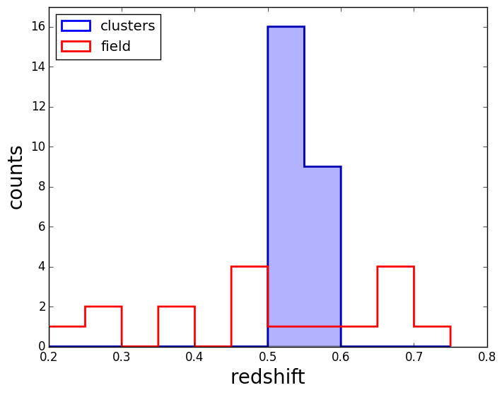
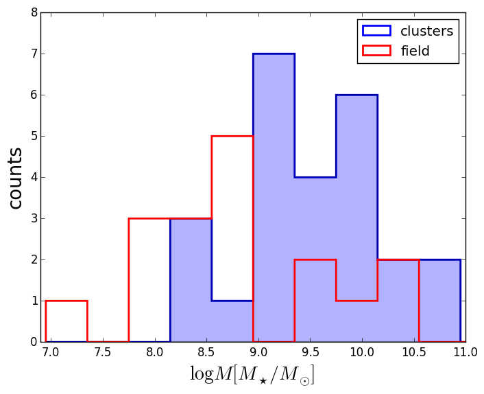
Figure 1.— Redshift (left) and mass (right) distributions for the cluster (blue, shade areas) and field (red) galaxies analyzed in this study.

We assemble a control sample which includes all galaxies with secure redshift, H$\alpha$ in emission detected in the G102 grism and redshift outside the cluster redshift intervals ($z<z_{cl}-0.03$ or $z>z_{cl}+0.03$). The field sample includes galaxies in the redshift range 0.2$<z<$0.7, and differences among these galaxies are therefore potentially due to evolutionary effects, although the average redshift is very similar between the two samples. We note that we do not have additional information on the environments in which these galaxies reside, therefore they might be located in some groups.

Overall, our sample includes 15 cluster members and 9 field galaxies from the MACS0717 field, and 10 cluster members and 8 field galaxies from the MACS1423 field.

Stellar masses have been estimated using the broad-band CLASH photometry (Postman et al., 2012) and a set of templates, computed with standard spectral synthesis models (Bruzual & Charlot, 2003), and fixing the redshift at the spectroscopic one. As it was done in previous papers (e.g., Fontana et al., 2004, 2006; Santini et al., 2015, for details), we have used a range of exponential time scales ranging from $0.1$ to $\infty$ Gyr. A Salpeter (1955) IMF, ranging over a set of metallicities (from Z = 0.02Z_⊙ to Z=2.5Z_⊙) and dust extinction (0¡E(B-V)¡1.1, with a Calzetti extinction curve) has been initially chosen, and then converted to a Kroupa (2001) IMF. We have also added emission lines in a self-consistent way, as described by Castellano et al. (2014), that provide an important contribution to our H$\alpha$-emitting galaxies. Uncertainties on the estimated masses have been derived by scanning (for each galaxy) all the templates and retaining only masses corresponding to models with $P(\chi^{2})>0.1$ (Santini et al., 2015).

Figure 1 shows the redshift and mass distribution for cluster and field samples separately. We note that, while the mass range spanned in the two environments is similar, going from 10⁸ to 10¹¹ M_⊙, the field galaxies are systematically less massive than cluster galaxies. Therefore, in the following, when comparing cluster and field populations, differences might be due to the different mass distribution, and not only to purely environmental effects.

3. Methodology

3.1. H$\alpha$ maps

The combined spatial resolution on the WFC3 and of the grism yield a spectrum that can be seen as images of a galaxy taken at $\sim$24 Å increments ($\sim$12 Å after interlacing) and placed next to each other (offset by one pixel) on the detector. Thus, an emission feature in a high spatial resolution slitless spectrum is essentially an image of a galaxy at that wavelength.

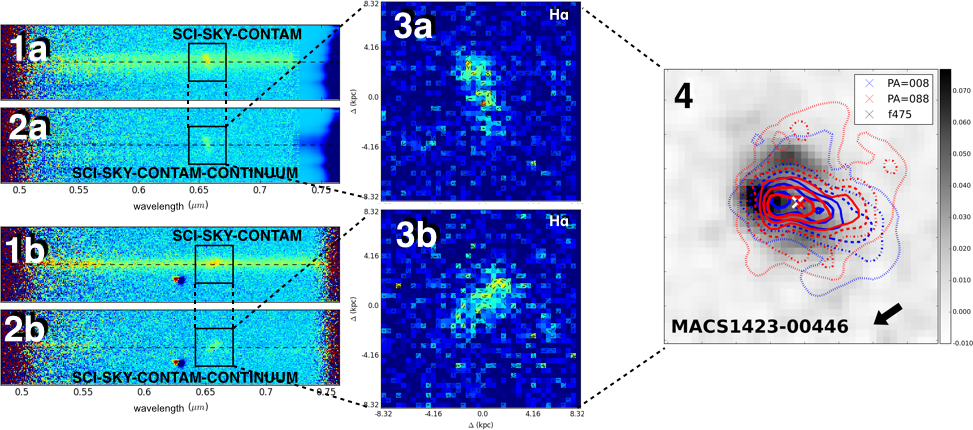
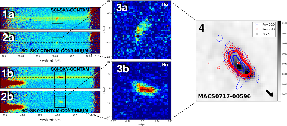
Figure 2.— Two examples of the procedure followed to derive $H_{\alpha}$ maps. Upper panels: MACS1423-00446, bottom panels: MACS0717-00596. $a$ and $b$ refer to the two distinct PAs of the same galaxy. Panels $1a$ and $1b$ show the rest-frame flux-calibrated galaxy 2D spectra, after the sky background and the contamination have been subtracted. The dashed horizontal black lines show the y-position of the continuum. The box shows the position of the emission lines. Panels $2a$ and $2b$ show the rest-frame 2D spectra after the continuum has also been subtracted. Panels $3a$ and $3b$ show the map of the galaxy in the light of the $H_{\alpha}$ line. Panels $4$ show the two maps overplotted as contours on an image of the galaxy in the FW475 filter. Blue and red lines represent different levels of $\Sigma$SFR, as described in Fig.5. The arrows indicates the direction of the cluster center. See text for details.

Figure 2 shows two examples of the procedure we followed to create H$\alpha$ emission line maps and therefore SFR maps. In the first steps, we treat the spectra coming from the different exposures (one per PA) of each galaxy independently, and only in the last step we combine them. Both panels $1a$ and $1b$ show the flux-calibrated galaxy 2D continuum spectra, after the sky background and the contamination have been subtracted. From two regions contiguous to the H$\alpha$ emission we determine the $y$-position of the peak of the continuum. This position will be needed to measure the offset in the $y$-direction of the H$\alpha$ emission with respect to the galaxy center in the light of the continuum. Subsequently, we subtract the 2D stellar continuum model obtained by convolving the best-fit 1D SED without emission lines with the actual 2D data, ensuring that all model flux pixels are non-negative (panels $2a$ and $2b$). If the sky, the contamination and the continuum were fit perfectly, we should be left only with the flux coming from the emission lines. We find that counts around the lines are slightly negative, suggesting that the continuum subtraction is somewhat too aggressive. Therefore, we select a box just above and one just below the emission line and measure the median flux which is further subtracted from the entire spectrum. The residual is a map of the galaxy in the light of the H$\alpha$ line (panels $3a$ and $3b$). As a last step, we superimpose the H$\alpha$ map onto an image of the galaxy taken with the F475W filter (rest-frame UV). We use F475W to map relatively recent ($\sim$100 Myr) star formation, as opposed to ongoing ($\sim$10Myr) star formation traced by H$\alpha$. To do so, we align each map to the image of the galaxy in the light of the continuum, rotating each map by the angle of its PA, keeping the $y$-offset unaltered with the respect to the continuum. On the $x$-axis, there is a degeneracy between the spatial dimension and the wavelength uncertainty, it is therefore not possible to determine very accurately the central position of the H$\alpha$ map for each PA separately. Nonetheless, for the cases in which spectra from both PAs are reliable (28/42), we use the fact that the 2 PAs differ by almost $90\degree$, therefore the $x$-direction of one spectrum roughly corresponds to the $y$-direction of the second spectrum and vice-versa. We can therefore shift the two spectra independently along their $x$-direction to force the center of the emission of the two maps to coincide. The results are shown in Figure 2, panels $4$. For the galaxies with reliable spectra in both PAs, we can also measure the real distance between the peak of the H$\alpha$ emission and the continuum emission, obtained as the quadratic sum of the two offsets.

Finally, for cluster galaxies, we also measure the magnitude of the offset between the H$\alpha$ and the continuum as projected along the cluster radial direction, determined by the line connecting the cluster-center and the galaxy center in the continuum light. We assign a positive sign to the projected offset when the peak of the H$\alpha$ is between the cluster center and the peak of the continuum.

3.2. H$\alpha$ map sizes

Since one of our aims is to compare the extent of H$\alpha$ light to the extent of the continuum light, we estimate galaxy sizes at different wavelengths by measuring the second order moment of the light distribution, which gives us the width of the distribution and therefore the extension of the galaxy:

$$\sigma=\sqrt{\frac{\sum_{i=1}^{N}\left[I(x_{i})\cdot x_{i}^{2}\right]}{\sum_{i=1}^{N}I(x_{i})}-\left[\frac{\sum_{i=1}^{N}\left[I(x_{i})\cdot x_{i}\right]}{\sum_{i=1}^{N}I(x_{i})}\right]^{2}}$$

with $x_{i}$ along the spectrum, and $I(x_{i})$ flux at the corresponding position. We measure sizes both along the $x-$ and $y-$direction. The average size is obtained by taking the mean of the two and summing errors in quadrature. This adopted size definition is independent on the galaxy’s center. When spectra from both PAs are reliable, we take the average size and sum the errors in quadrature, after having checked that the measurements from the two PAs are consistent within the uncertainty.

Besides on the H$\alpha$ light, we compute sizes both on the F475W filter, to map the star formation occurred in roughly the last 100 Myr, and on the F110W filter, which probes the rest-frame optical continuum and therefore maps the older stellar population. We correct our size estimates for the point spread function (PSF) of our observations. We estimate the mean full width half maximum (FWHM) in each band by taking the average of the FWHM of 5 stars. We then subtract in quadrature the PSF (=FWHM/2.355) from the sizes. The values we obtain are $\sim$0.03^′′ in the F475W, and $\sim$0.055^′′ in the F110W and G102 filters. We note that the PSF correction is generally much smaller than the sizes we observe therefore the impact of the correction is negligible.

We note that more robust measurements are currently underway for the entire GLASS sample and will be presented in a forthcoming paper.

Table 2Properties of galaxies in clusters

obj_name	RA	DEC	z	$\log$ M	EW	SFR	$\Sigma$SFR	dist${}_{r_{500}}$	dist
	(J2000)	(J2000)		(M⊙)		(M${}_{\odot}/yr$)	(M${}_{\odot}/yr/kpc^{2}$)		(kpc)
MACS0717-00173	07:17:35.64	+37:45:59.2	0.556	9.5${}^{+0.4}_{-0.5}$	23$\pm$2	3.4$\pm$0.5	0.20$\pm$0.03	0.276	466
MACS0717-00234	07:17:35.14	+37:45:52.9	0.549	10.5${}^{+0.1}_{-0.3}$	14.1$\pm$0.3	8.6$\pm$0.8	0.16$\pm$0.01	0.247	418
MACS0717-00431	07:17:36.59	+37:45:40.1	0.5495	8.9${}^{+0.2}_{-0.3}$	29$\pm$3	2.9$\pm$0.4	0.30$\pm$0.06	0.226	382
MACS0717-00596	07:17:37.76	+37:45:30.1	0.5475	9.9${}^{+0.2}_{-0.4}$	65$\pm$2	14.0$\pm$0.6	0.54$\pm$0.03	0.230	388
MACS0717-00624	07:17:33.44	+37:45:28.9	0.5725	9.0${}^{+0.1}_{-0.3}$	35$\pm$4	2.3$\pm$0.5	0.15$\pm$0.04	0.153	259
MACS0717-00674	07:17:34.98	+37:45:27.4	0.574	9.3${}^{+0.2}_{-0.2}$	24$\pm$5	0.8$\pm$0.4	0.08$\pm$0.06	0.152	257
MACS0717-00977	07:17:38.86	+37:45:20.0	0.567	9.3${}^{+0.2}_{-0.3}$	18.5$\pm$0.6	4.8$\pm$0.7	0.10$\pm$0.02	0.248	419
MACS0717-01208	07:17:32.79	+37:44:41.3	0.5585	9.5${}^{+0.3}_{-0.7}$	63$\pm$5	5.1$\pm$0.4	0.53$\pm$0.06	0.062	105
MACS0717-01305	07:17:35.55	+37:44:41.8	0.5285	10.7${}^{+0.2}_{-0.2}$	18.1$\pm$0.5	18$\pm$1	0.14$\pm$0.01	0.074	1256
MACS0717-02181	07:17:31.51	+37:44:13.1	0.564	9.0${}^{+0.1}_{-0.4}$	11$\pm$4	1.3$\pm$0.4	0.16$\pm$0.07	0.176	298
MACS0717-02189	07:17:33.76	+37:44:08.4	0.5275	10.0${}^{+0.3}_{-0.4}$	6.2$\pm$0.2	3.0$\pm$0.6	0.17$\pm$0.06	0.154	260
MACS0717-02297	07:17:30.17	+37:44:04.1	0.5485	9.2${}^{+0.3}_{-0.3}$	19$\pm$1	3.1$\pm$0.4	0.28$\pm$0.04	0.242	408
MACS0717-02334	07:17:32.35	+37:43:59.4	0.534	9.9${}^{+0.2}_{-0.2}$	13.8$\pm$0.3	7.4$\pm$0.5	0.35$\pm$0.03	0.202	341
MACS0717-02432	07:17:31.45	+37:43:50.7	0.548	9.4${}^{+0.4}_{-0.3}$	55$\pm$9	2.9$\pm$0.5	0.17$\pm$0.03	0.249	420
MACS0717-02574	07:17:31.76	+37:43:33.8	0.5375	10.2${}^{+0.6}_{-0.4}$	29$\pm$1	9.1$\pm$0.7	0.25$\pm$0.02	0.302	511
MACS1423-00152	14:23:49.65	+24:05:43.0	0.53	9.0${}^{+0.2}_{-0.3}$	21$\pm$2	2.0$\pm$0.4	0.15$\pm$0.03	0.345	376
MACS1423-00229	14:23:46.25	+24:05:32.6	0.563	8.3${}^{+0.1}_{-0.1}$	110$\pm$30	4.1$\pm$0.5	0.28$\pm$0.05	0.313	342
MACS1423-00310	14:23:45.62	+24:05:27.3	0.53	9.9${}^{+0.2}_{-0.4}$	26$\pm$1	3.7$\pm$0.5	0.26$\pm$0.05	0.319	348
MACS1423-00319	14:23:48.24	+24:05:20.7	0.536	10.4${}^{+0.2}_{-0.5}$	36$\pm$4	3.0$\pm$0.7	0.12$\pm$0.03	0.198	215
MACS1423-00446	14:23:45.18	+24:05:16.4	0.548	9.9${}^{+0.3}_{-0.4}$	57$\pm$2	8.7$\pm$0.6	0.40$\pm$0.04	0.304	331
MACS1423-00487	14:23:47.81	+24:05:13.6	0.53	9.7${}^{+0.3}_{-0.4}$	61$\pm$5	7.1$\pm$0.6	0.38$\pm$0.03	0.161	175
MACS1423-00831	14:23:49.24	+24:04:52.3	0.575	8.5${}^{+0.9}_{-0.5}$	41$\pm$4	2.6$\pm$0.5	0.11$\pm$0.03	0.081	89
MACS1423-01516	14:23:48.56	+24:04:14.6	0.54	10.6${}^{+0.2}_{-0.3}$	27.1$\pm$0.3	14.8$\pm$0.7	0.48$\pm$0.03	0.190	208
MACS1423-01253	14:23:53.13	+24:04:29.4	0.556	9.1${}^{+0.1}_{-0.2}$	13$\pm$1	2.4$\pm$0.5	0.12$\pm$0.02	0.400	437
MACS1423-01910	14:23:49.20	+24:03:42.7	0.532	8.5${}^{+0.2}_{-0.3}$	100$\pm$10	3.2$\pm$0.4	0.35$\pm$0.06	0.383	418

Table 3Spatial properties of galaxies in clusters

obj_name	offset 1	offset 2	r(H$\alpha$)x	r(H$\alpha$)y	r(F110W)x	r(F110W)y	r(F475W)x	r(F475W)y	A	B	$\theta$
	(kpc)	(kpc)	(kpc)	(kpc)	(kpc)	(kpc)	(kpc)	(kpc)	(kpc)	(kpc)	(deg)
MACS0717-00173	-	0.4$\pm$0.1	4.1$\pm$0.3	1.0$\pm$0.2	1.63	0.82	3.77	1.24	3.25	1.62	-47.6
MACS0717-00234	-	-0.4$\pm$0.1	3.7$\pm$0.5	2.0$\pm$0.8	3.37	2.44	3.17	2.13	5.32	3.2	-16.3
MACS0717-00431	-0.43$\pm$0.1	0.18$\pm$0.07	1.38$\pm$0.09	1.0$\pm$0.2	1.09	0.98	1.62	1.45	1.81	1.61	17.4
MACS0717-00596	0.11$\pm$0.05	-0.16$\pm$0.03	3.2$\pm$0.4	2.6$\pm$0.3	2.84	1.82	3.39	2.22	3.5	2.39	-61.8
MACS0717-00624	-0.4$\pm$0.2	-0.5$\pm$0.3	3.7$\pm$0.8	4$\pm$1	1.88	1.20	0.80	0.54	2.58	1.83	-81.5
MACS0717-00674	0.2$\pm$0.4	0.7$\pm$0.3	4.3$\pm$0.3	3$\pm$1	2.28	2.11	5.69	6.28	1.96	1.51	-58.4
MACS0717-00977	-	0.1$\pm$0.2	3.3$\pm$0.7	3.7$\pm$0.6	3.06	2.71	3.67	3.45	4.28	3.55	-80.3
MACS0717-01208	-0.19$\pm$0.07	0.31$\pm$0.04	3.9$\pm$0.6	3.2$\pm$0.5	3.20	3.11	1.64	1.95	1.95	1.57	-44.7
MACS0717-01305	-1.6$\pm$0.1	-1.0$\pm$0.2	3.1$\pm$0.3	2.9$\pm$0.4	3.71	3.73	3.57	3.12	7.06	5.4	23.5
MACS0717-02181	-0.2$\pm$0.2	0.1$\pm$0.2	4$\pm$1	3.7$\pm$0.9	1.07	0.91	-	4.61	1.68	1.52	-47.0
MACS0717-02189	-1.9$\pm$0.3	-0.1$\pm$0.1	3.2$\pm$0.3	2.7$\pm$0.4	2.98	3.06	3.05	1.40	3.5	1.5	-55.1
MACS0717-02297	-0.06$\pm$0.09	-	2$\pm$1	1.5$\pm$0.6	0.94	0.97	2.89	1.40	2.01	1.7	-14.1
MACS0717-02334	-	0.62$\pm$0.05	1$\pm$1.0	1.7$\pm$0.6	2.77	2.14	2.23	1.52	3.35	2.02	-74.7
MACS0717-02432	0.4$\pm$0.2	-	1$\pm$1	0.8$\pm$0.1	2.68	0.59	2.89	0.73	3.69	1.48	-80.5
MACS0717-02574	0.11$\pm$0.09	-	3.6$\pm$0.3	3.5$\pm$0.3	-	-	3.93	1.25	7.34	1.57	-74.0
MACS1423-00152	-0.2$\pm$0.2	-	6$\pm$2	5$\pm$2	1.16	1.12	0.98	1.03	0.71	0.61	3.1
MACS1423-00229	0.23$\pm$0.08	-0.1$\pm$0.1	4.4$\pm$0.4	3$\pm$1	3.09	1.68	3.01	0.61	1.28	1.05	-6.0
MACS1423-00310	0.16$\pm$0.07	0.5$\pm$0.2	4.2$\pm$0.5	2.8$\pm$0.7	2.02	2.10	1.85	2.49	2.17	1.96	16.7
MACS1423-00319	-	0.11$\pm$0.09	4.5$\pm$0.5	5.0$\pm$0.5	2.92	2.14	1.11	0.84	3.65	3.18	4.0
MACS1423-00446	-0.28$\pm$0.05	-0.18$\pm$0.06	3.2$\pm$0.3	3.3$\pm$0.3	2.60	1.95	2.92	2.09	6.71	2.56	86.4
MACS1423-00487	-	0.42$\pm$0.07	3.1$\pm$0.3	1.4$\pm$0.1	3.03	1.72	1.90	0.89	0.81	0.44	-55.4
MACS1423-00831	-0.1$\pm$0.2	-0.2$\pm$0.3	4.1$\pm$0.6	4.9$\pm$0.5	3.06	1.75	1.88	1.13	1.0	0.8	-12.0
MACS1423-01253	-0.0$\pm$0.2	-	4.0$\pm$0.8	3.2$\pm$0.9	2.09	1.75	1.25	1.09	2.59	1.73	70.7
MACS1423-01516	-0.29$\pm$0.04	-0.76$\pm$0.06	3.8$\pm$0.2	3.7$\pm$0.2	2.50	2.33	2.83	2.90	1.57	1.37	75.6
MACS1423-01910	-0.15$\pm$0.05	0.5$\pm$0.1	2$\pm$1	4$\pm$1	1.62	1.16	1.45	1.90	0.68	0.53	22.1

Table 4Properties of galaxies in the field

obj_name	RA	DEC	z	$\log$ M	EW	SFR	$\Sigma$SFR
	(J2000)	(J2000)		(M⊙)		(M${}_{\odot}/yr$)	(M${}_{\odot}/yr/kpc^{2}$)
MACS0717-00236	07:17:34.48	+37:45:52.1	0.39	10.2${}^{+0.3}_{-0.3}$	11.3$\pm$0.2	15$\pm$1	0.29$\pm$0.03
MACS0717-00450	07:17:37.39	+37:45:34.9	0.5965	8.5${}^{+0.2}_{-0.5}$	90$\pm$40	2.4$\pm$0.5	0.13$\pm$0.04
MACS0717-01234	07:17:37.56	+37:45:09.3	0.2295	8.1${}^{+0.3}_{-0.3}$	110$\pm$10	7.2$\pm$1.6	0.6$\pm$0.2
MACS0717-01416	07:17:39.72	+37:44:50.7	0.5095	9.7${}^{+0.3}_{-0.3}$	32$\pm$1	6.0$\pm$0.4	0.51$\pm$0.03
MACS0717-01477	07:17:29.74	+37:44:46.2	0.45	9.5${}^{+0.1}_{-0.3}$	9.6$\pm$0.6	9$\pm$1	0.13$\pm$0.02
MACS0717-01589	07:17:32.33	+37:44:37.6	0.385	8.0${}^{+0.9}_{-0.1}$	40$\pm$2	10$\pm$1	0.24$\pm$0.02
MACS0717-02371	07:17:31.95	+37:44:01.7	0.263	8.8${}^{+0.3}_{-0.5}$	17$\pm$3	2.7$\pm$0.8	0.4$\pm$0.2
MACS0717-02390	07:17:34.63	+37:43:53.8	0.473	8.7${}^{+0.1}_{-0.2}$	35$\pm$2	6$\pm$1	0.17$\pm$0.05
MACS0717-02445	07:17:32.38	+37:43:51.0	0.49	8.7${}^{+0.1}_{-0.2}$	90$\pm$30	2.8$\pm$0.5	0.20$\pm$0.06
MACS1423-00246	14:23:49.68	+24:05:33.6	0.66	7.0${}^{+0.9}_{-0.7}$	70$\pm$50	0.4$\pm$0.2	0.12$\pm$0.06
MACS1423-00256	14:23:45.35	+24:05:31.4	0.71	7.8${}^{+0.8}_{-0.5}$	-	0.2$\pm$0.2	0.1$\pm$0.1
MACS1423-00463	14:23:46.44	+24:05:15.4	0.62	8.5${}^{+0.3}_{-0.1}$	77$\pm$9	1.8$\pm$0.4	0.13$\pm$0.03
MACS1423-00610	14:23:49.10	+24:05:02.6	0.655	10.3${}^{+0.2}_{-0.3}$	24.3$\pm$0.5	9.0$\pm$0.7	0.22$\pm$0.02
MACS1423-00677	14:23:45.68	+24:04:55.2	0.665	8.9${}^{+0.2}_{-0.2}$	49$\pm$5	4.3$\pm$0.4	0.33$\pm$0.05
MACS1423-01729	14:23:46.13	+24:04:00.2	0.455	8.7${}^{+0.4}_{-0.4}$	42$\pm$4	3.4$\pm$0.5	0.28$\pm$0.06
MACS1423-01771	14:23:44.43	+24:03:56.1	0.65	10.1${}^{+0.2}_{-0.2}$	38$\pm$1	11.8$\pm$0.7	0.34$\pm$0.02
MACS1423-01972	14:23:48.07	+24:03:34.6	0.278	8.3${}^{+0.5}_{-0.3}$	140$\pm$50	3.4$\pm$0.6	0.9$\pm$0.2

Table 5Spatial properties of galaxies in the field

obj_name	offset 1	offset 2	r(H$\alpha$)x	r(H$\alpha$)y	r(F110W)x	r(F110W)y	r(F475W)x	r(F475W)y	A	B	$\theta$
	(kpc)	(kpc)	(kpc)	(kpc)	(kpc)	(kpc)	(kpc)	(kpc)	(kpc)	(kpc)	(deg)
MACS0717-00236	0.1$\pm$0.1	0.6$\pm$0.1	3.8$\pm$0.1	3.3$\pm$0.2	3.09	2.62	3.39	2.85	4.85	3.59	47.9
MACS0717-00450	-2.2$\pm$0.5	0.8$\pm$0.2	3.2$\pm$0.5	0.8$\pm$0.2	3.76	0.83	3.72	3.82	3.14	1.85	4.8
MACS0717-01234	0$\pm$1	0.3$\pm$0.2	2$\pm$2	0.7$\pm$0.2	1.27	1.13	1.12	1.01	2.88	1.31	76.2
MACS0717-01416	-	-0.24$\pm$0.05	5$\pm$1	5$\pm$1	-	-	2.25	2.56	1.94	1.82	-0.9
MACS0717-01477	-1.3$\pm$0.3	-0.2$\pm$0.2	3.5$\pm$0.4	3.7$\pm$0.3	3.29	2.90	3.50	3.29	5.29	4.08	-19.3
MACS0717-01589	-	-0.1$\pm$0.1	2.4$\pm$0.7	1$\pm$1	3.29	3.37	3.40	3.59	3.91	3.5	-29.1
MACS0717-02371	0.4$\pm$0.4	-0.1$\pm$0.7	1.4$\pm$0.6	1.5$\pm$0.9	0.63	1.04	0.69	0.89	1.34	1.15	-27.2
MACS0717-02390	0.1$\pm$0.1	0.1$\pm$0.1	1.5$\pm$0.8	0.9$\pm$0.1	2.03	1.63	3.90	2.72	6.32	3.36	-86.5
MACS0717-02445	0.1$\pm$0.1	-0.1$\pm$0.3	4$\pm$1	3$\pm$1	1.61	0.48	2.88	0.96	2.43	1.25	-77.7
MACS1423-00246	-0.2$\pm$0.2	-	-	5$\pm$1	-	-	5.67	7.03	0.7	0.44	-77.6
MACS1423-00256	-	-1.2$\pm$0.7	-	0.9$\pm$0.3	1.41	4.48	4.35	2.51	2.63	2.27	-11.5
MACS1423-00463	0.3$\pm$0.2	-	34$\pm$1	3$\pm$2	2.43	2.36	2.14	1.46	1.58	0.86	32.7
MACS1423-00610	-1.2$\pm$0.1	0.11$\pm$0.09	4.0$\pm$0.3	3.2$\pm$0.3	3.59	2.53	3.79	2.32	1.72	0.71	74.3
MACS1423-00677	0.01$\pm$0.05	-0.3$\pm$0.1	4.0$\pm$0.3	3.6$\pm$0.4	2.17	1.73	2.16	3.52	1.34	1.17	20.5
MACS1423-01729	-0.1$\pm$0.1	-0.7$\pm$0.2	3$\pm$1	3.4$\pm$0.6	1.86	1.65	1.88	1.81	1.84	1.43	47.5
MACS1423-01771	-	0.07$\pm$0.07	3.7$\pm$0.3	3.4$\pm$0.3	3.12	2.84	3.35	3.26	4.22	2.49	34.3
MACS1423-01972	0.2$\pm$0.1	-0.1$\pm$0.1	2.3$\pm$0.8	0.9$\pm$0.3	0.78	1.19	1.21	1.25	4.05	1.67	-40.8

3.3. SFRs and EW(H$\alpha$)s

From the H$\alpha$ maps we also derive SFRs. We use the conversion factor derived by Kennicutt, Tamblyn & Congdon (1994) and Madau, Pozzetti & Dickinson (1998):

$$\textrm{SFR}[\textrm{M}_{\odot}\,\textrm{yr}^{-1}]=5.5\times 10^{-42}\textrm{L}(H\alpha)[\textrm{erg}\,\textrm{s}^{-1}]$$

valid for a Kroupa (2001) IMF. We compute both the surface SFR density ($\Sigma$SFR, $\textrm{M}_{\odot}\,\textrm{yr}^{-1}\,\textrm{kpc}^{-2}$) and the total SFRs ($\textrm{M}_{\odot}\,\textrm{yr}^{-1}$), separately for the spectra coming from the two PAs and then we combine them taking the mean values. Errors are summed in quadrature. The total SFRs are obtained summing the surface SFR density within the Kron radius of the galaxy.

There are two major limitations when using H$\alpha$ as SFR estimator: the contamination by the [NII] line doublet, and uncertainties in the extinction corrections to be applied to each galaxy.

To correct for the scatter due to the [NII] contamination, we apply the locally calibrated correction factor given by James et al. (2005). As opposed to previous works which considered only central regions, these authors developed a method which takes into account the variation of the H$\alpha$/[NII] with radial distance from the galaxy center, finding an average value of H$\alpha$/(H$\alpha$ + [NII])= 0.823. This approach is appropriate given our goal to investigate extended emission.

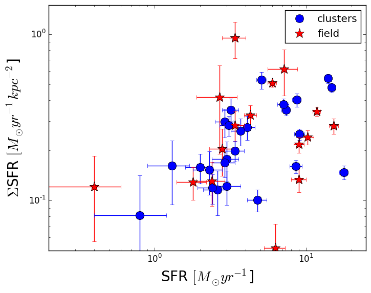
Figure 3.— $\Sigma$SFR-SFR for cluster (blue) and field (red) galaxies in our sample.

The second major problem when deriving SFR(H$\alpha$) is the effect of dust extinction. Star formation normally takes place in dense and dusty molecular clouds, so a significant fraction of the emitted light from young stars is absorbed by the dust and re-emitted at rest-frame IR wavelengths. Hopkins et al. (2001) modeled a SFR-dependent attenuation by dust, characterized by the Calzetti reddening curve of the form

$$\log(\textrm{SFR}_{i})=\log(\textrm{SFR}_{o}(H\alpha))+2.614\times$$

$$\log\left[\frac{0.797\times\log(\textrm{SFR}_{i})+3.834}{2.88}\right]$$

which allows us to estimate attenuation and intrinsic SFR, even for observations of a single H$\alpha$ emission line. We use this correction to obtain the intrinsic SFRs.

Figure 3 correlates the total $\Sigma$SFRs to the SFR and shows that our $\Sigma$SFR limit is around $10^{-1}$ M_⊙ yr^-1 kpc^-2 for SFR$\sim 1M_{\odot}yr^{-1}$.

Finally, we also compute H$\alpha$ equivalent widths (EW(H$\alpha$)) from the collapsed 2D spectra. We define the line profile by adopting a fixed rest frame wavelength range, centered on the theoretical wavelength, 6480-6650 Å, and then obtain the line flux, $f_{\textrm{line}}$, by summing the flux within the line. The continuum is defined by two regions of 100 Å located at the two extremes of the line profile. We fit a straight line to the average continuum in the two regions and sum the flux below the line, to obtain $f_{\textrm{cont}}$. The rest-frame EW(H$\alpha$) is therefore defined by

$$\textrm{EW}(H_{\alpha})=\frac{f_{\textrm{line}}}{f_{\textrm{cont}}\times(1+z)}$$

We note that our approach ignores underlying H$\alpha$ absorption. As usual, when two spectra for the same galaxy are reliable, the final value is given by the average of the two EW estimates, and the error is obtained by summing in quadrature the individual errors. The measurements from the two PAs are consistent within the uncertainty. Otherwise we just use a single spectrum.

4. Results

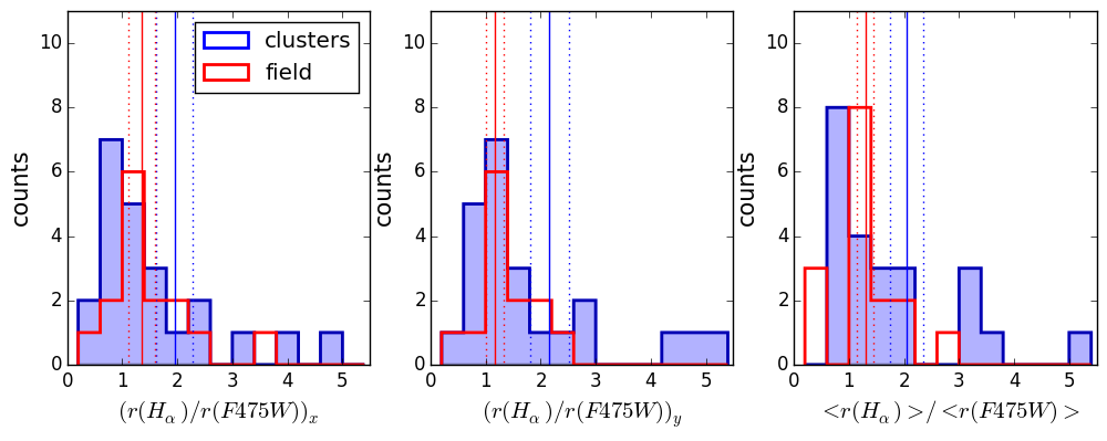
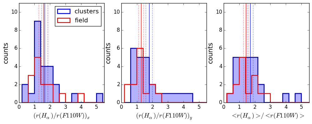
Figure 4.— Distribution of the ratio of the size of the H$\alpha$ emission to the size as measured from the F475W filter (upper panel) and from the F110W filter (bottom panel). Left and central panels show the sizes in the two directions separately, right panel shows the mean size. Vertical solid and dotted lines represent the means with errors. Both in clusters and in the field mean values are larger than 1, suggesting the inside-out growth, but when using the F475W, tracer of the recent star formation, in clusters mean values are even larger, pointing at cluster specific processes at work.

Tables 2 to 5 summarize the properties of the galaxies in our cluster and field samples, respectively. They include galaxy positions, redshifts, stellar masses, EW(H$\alpha$)s, SFRs, $\Sigma$SFRs, sizes in different bands (F475W, F110W and H$\alpha$) along both the $x-$ and $y-$ direction, the offset between the peak of the light in H$\alpha$ and in the rest-frame UV continuum, and, for clusters, the cluster-centric distances (both in kpc and in units of $r_{500}$).

Figure 4 shows the distribution of the ratio of the size as measured from the H$\alpha$ light (r(H$\alpha$)) to the size as measured from the rest-frame UV continuum (r(F745W)) and rest-frame optical continuum (r(F110W)), both for the two directions separately and for the mean sizes, obtained as average between the two directions. We therefore compare the currently star forming regions to the younger stellar population (traced by the observed F475W continuum) and to the older one (traced by the observed F110W continuum). In a forthcoming analysis we will also compare H$\alpha$ maps to maps of the even older stellar populations, as traced by the rest-frame Infrared.

In both environments, there is no preferential axis for the H$\alpha$ emission. Ratios obtained using the F110W and the F475W filters agrees within the errors, in both clusters and field. Looking at the continuum sizes, we do not detect strong trends with the wavelengths, most likely because of the our currently small number statistics. Distributions peak around 1, showing that many galaxies have comparable sizes in the line and continuum. However, distributions are slightly skewed toward values $>1$. In cluster galaxies mean size ratios are systematically slightly larger than field galaxies when the F475W is used, but not when the F110W filter is considered (clusters: $(r(H\alpha)/r(F475W))_{x}=1.8\pm 0.3$, $(r(H\alpha)/r(F475W))_{y}=2.2\pm 0.3$, $\langle r(H\alpha)\rangle/\langle r(F745W)\rangle=1.9\pm 0.3$; $(r(H\alpha)/r(F110W))_{x}=1.6\pm 0.2$, $(r(H\alpha)/r(F110W))_{y}=1.8\pm 0.2$, $\langle r(H\alpha)\rangle/\langle r(F1110W)\rangle=1.7\pm 0.2$; field: ($r(H\alpha)/r(F475W))_{x}=1.3\pm 0.2$, $(r(H\alpha)/r(F475W))_{y}=1.2\pm 0.2$, $\langle r(H\alpha)\rangle/\langle r(F745W)\rangle=1.3\pm 0.1$; $(r(H\alpha)/r(F110W))_{x}=1.6\pm 0.3$, $(r(H\alpha)/r(F110W))_{y}=1.6\pm 0.2$, $\langle r(H\alpha)\rangle/\langle r(F110W)\rangle=1.4\pm 0.1$). Mean values for cluster galaxies are driven by a subpopulation of galaxies ($\sim$ 20%) which present H$\alpha$ emission at least two-three time as extended as the light in the rest-frame UV continuum. No such examples are present in the field. This might suggest that in all environments star formation is probably occurring over a larger area than that of the recent star formation ($\sim 100$ Myr), but in clusters there might be some additional mechanisms that are stripping the gas and star formation is continuing in the stripped material. A Kolomgorov-Smirnov (K-S) test can not reject the hypothesis that the distributions of the two samples are the same, giving probabilities lower than 80% in all the three cases. We note that both samples are quite small, which might explain why the K-S test is inconclusive.

We use the information in the top right panel of Fig. 4 to group galaxies into different classes, as described in the next subsection.

4.1. Maps of H$\alpha$ and continuum emission

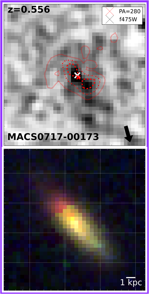
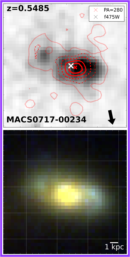
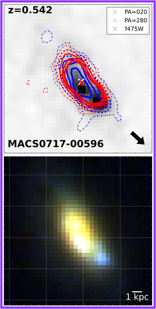
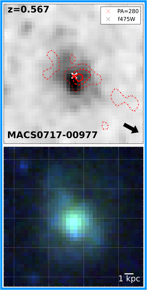
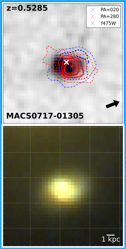
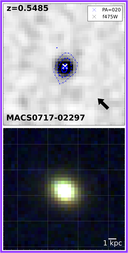
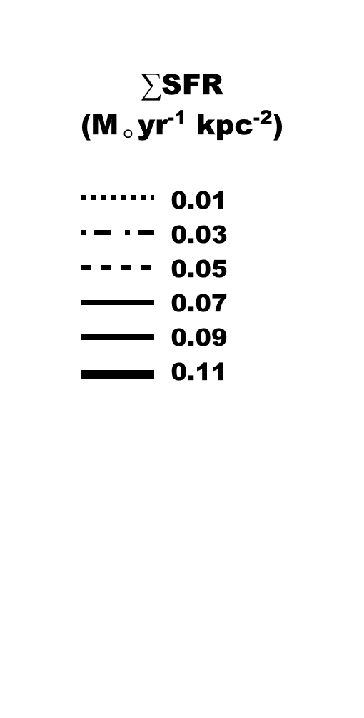
Figure 5.— Cluster galaxies with $0.8<\langle r($H$\alpha$ $)\rangle/\langle r(F745W)\rangle<1.2$. For each galaxy, in the upper panel the contour plots showing the H$\alpha$ maps superimposed on the image of the galaxy in the F475W filter are shown, in the bottom panel the color composite image of the galaxy based on the CLASH (Postman et al., 2012) HST data is shown. The blue channel is composed by the F435W, F475W, F555W, F606W, and F625W (the last one only for MACS0717) filters, the green by the F775W, F814W, F850lp, F105W, F110W filters, and the red by the F125W, F140W, F160W filters. In the H$\alpha$ maps, different colors refer to the different PAs, Different line styles are indicated in the legend. A smoothing filter has been applied to the maps and an arbitrary stretch to the images for display purposes. for Purple lines surround elongated galaxies (axis ratio in the F475W filter $\neq 1\pm 0.2$) light blue lines surround symmetric galaxies (axis ratio in the F475W filter $\sim 1\pm 0.2$). Arrows on the bottom right corner indicate the direction of the cluster center. The redshift of the galaxy is indicated on the top left corner.

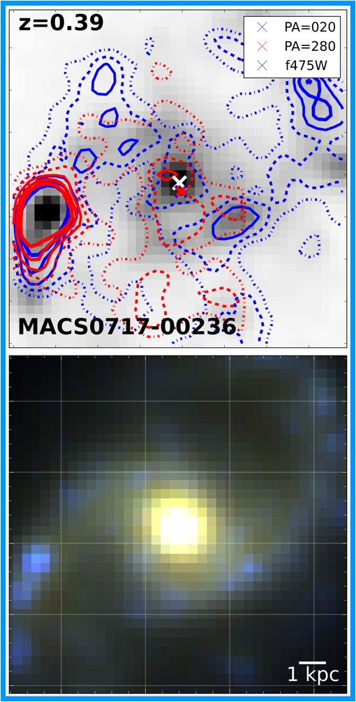
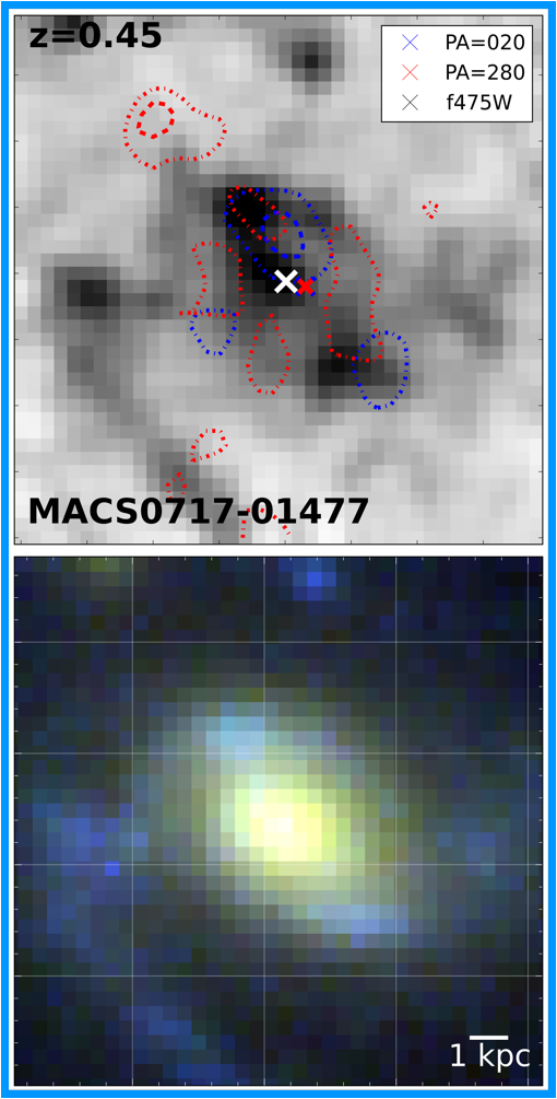
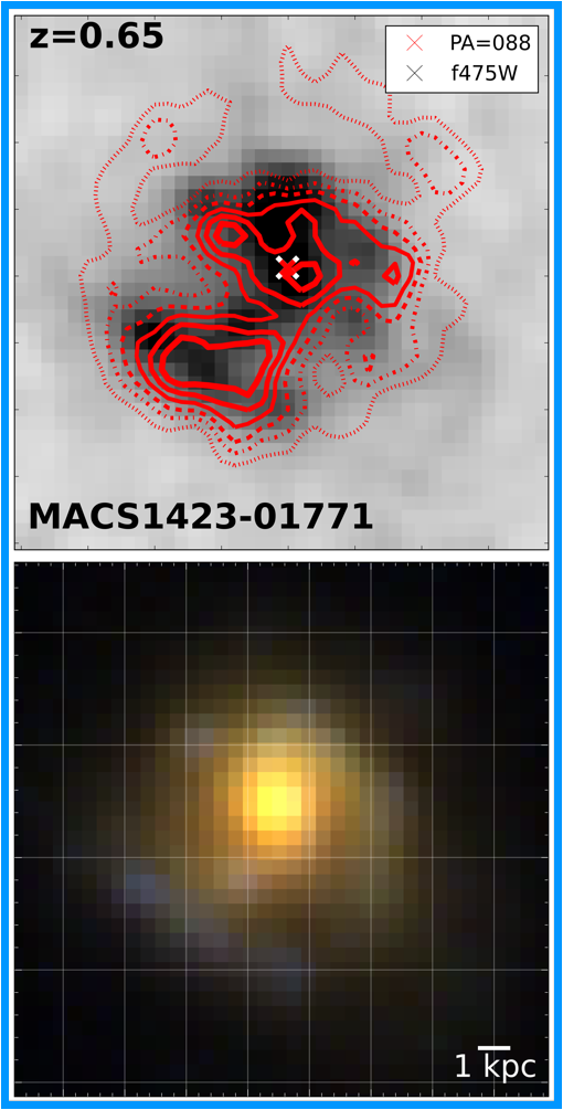
Figure 6.— Field galaxies with $0.8<\langle r($H$\alpha$ $)\rangle/\langle r(F745W)\rangle<1.2$. Panels, lines and colors are as in Fig. 5.

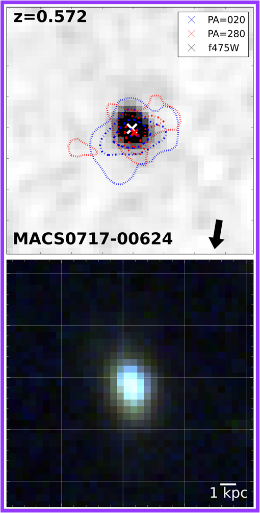
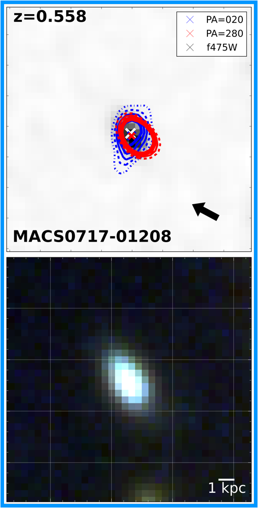
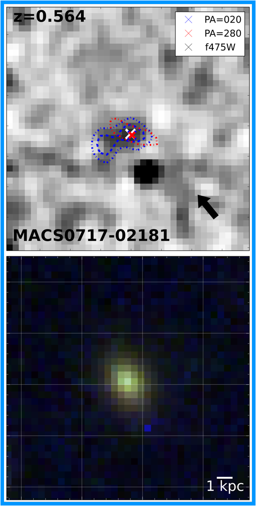
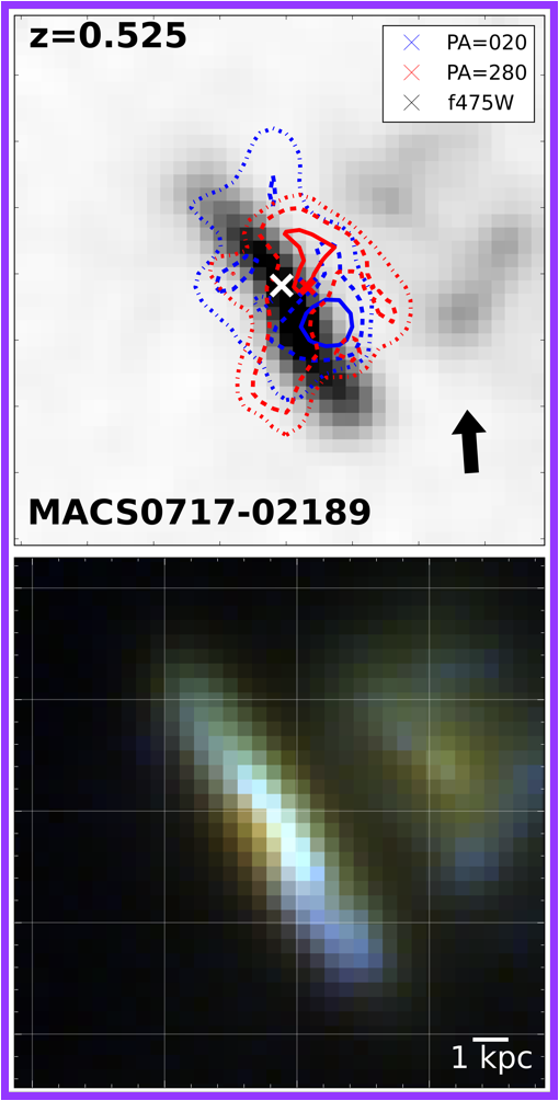
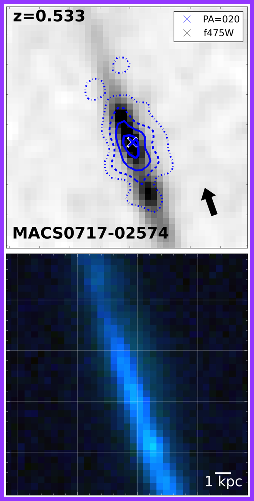
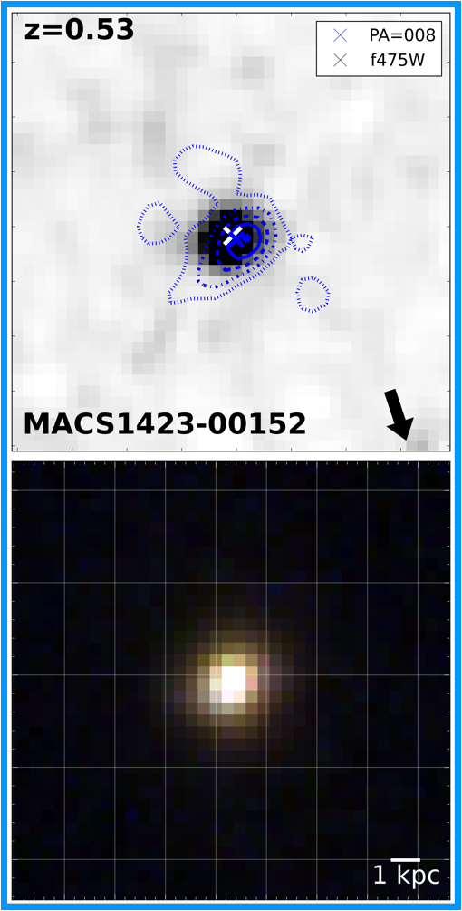
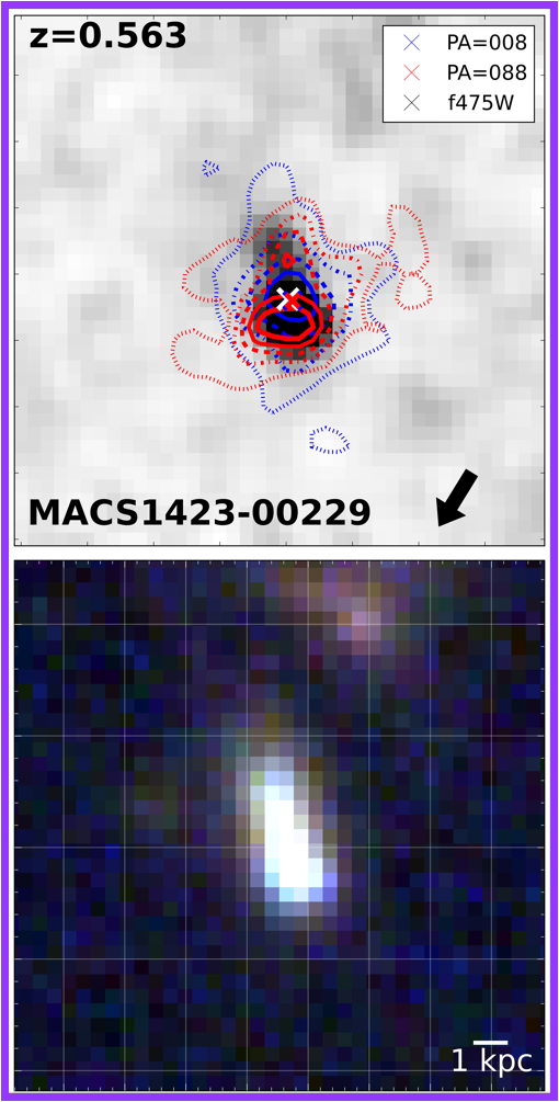
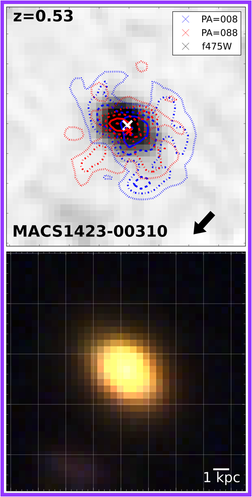
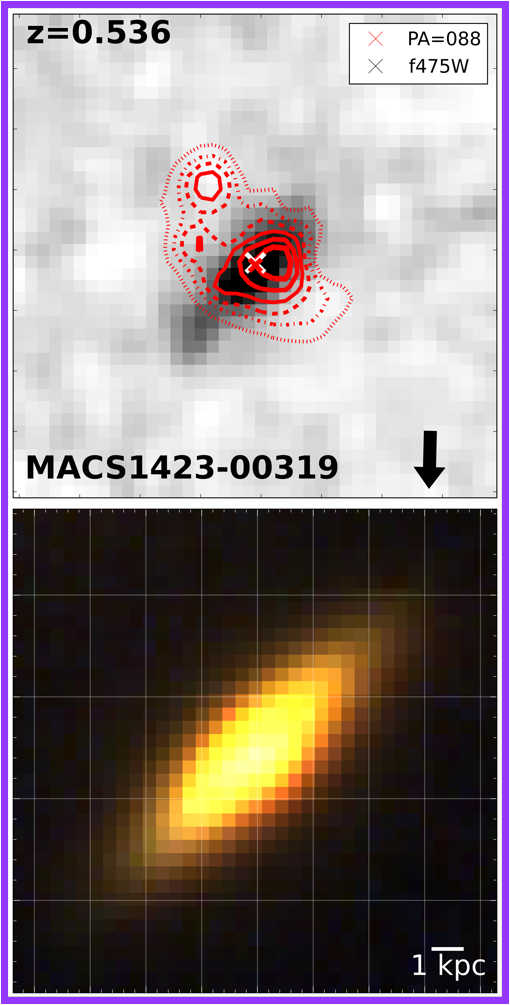
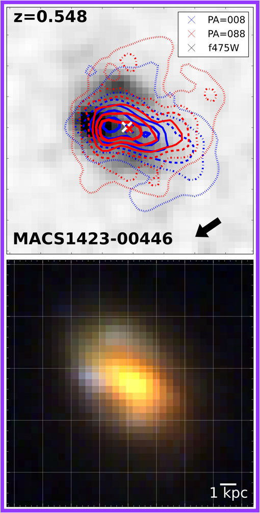
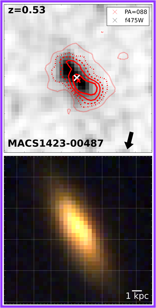
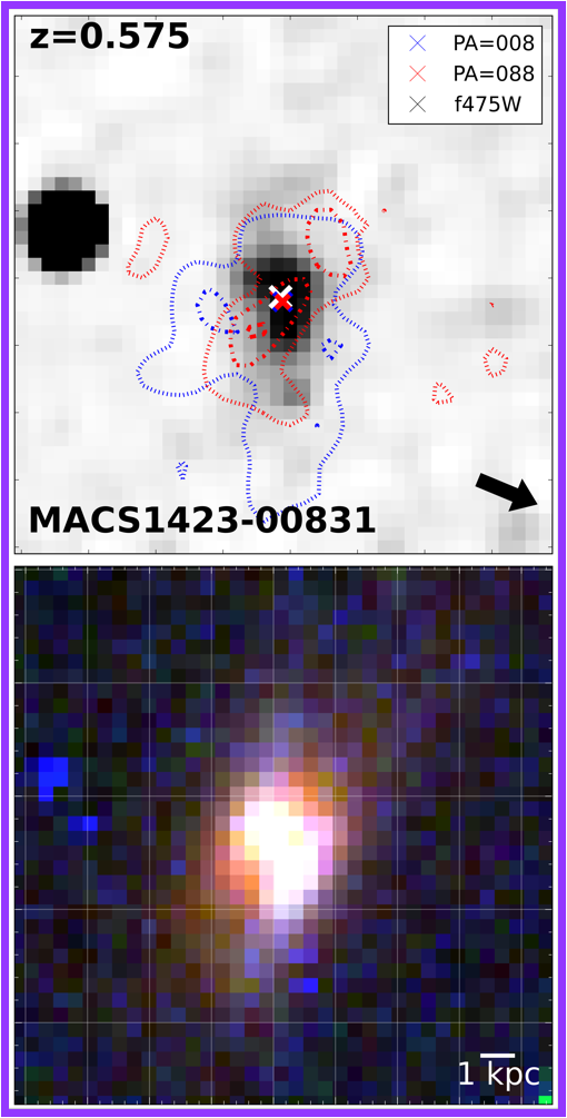
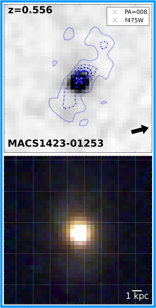
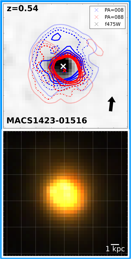
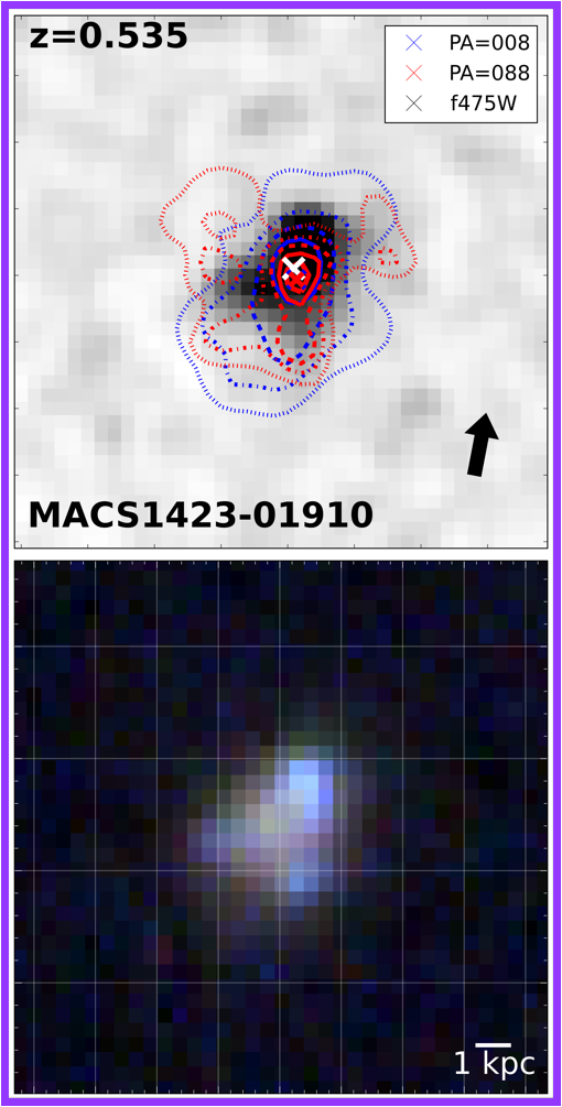
Figure 7.— Cluster galaxies with $\langle r($H$\alpha$ $)\rangle/\langle r(F745W)\rangle>1.2$. Panels, lines and colors are as in Fig. 5.

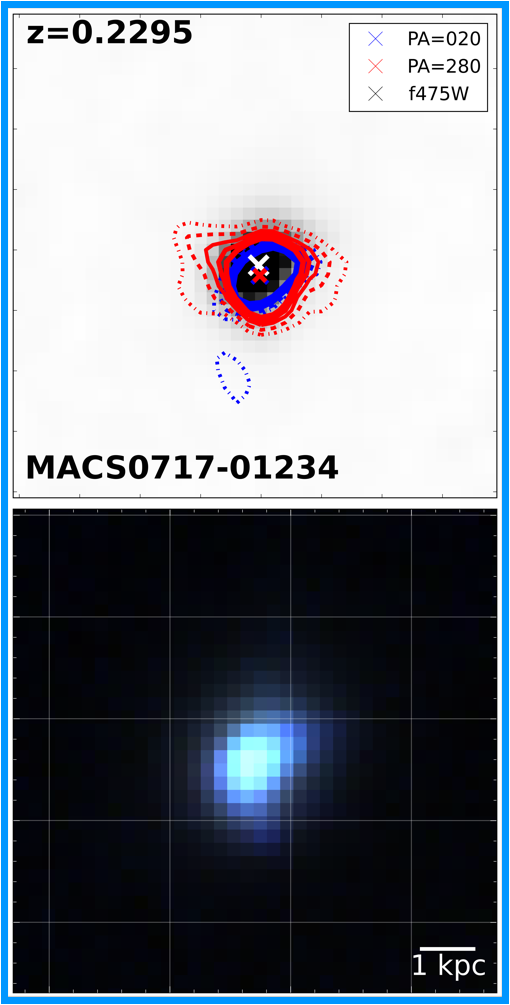
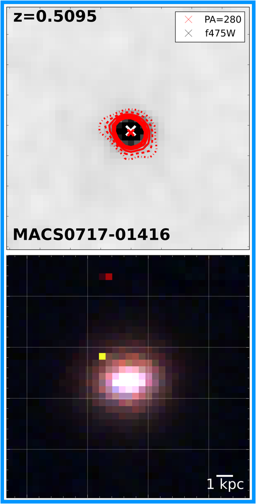
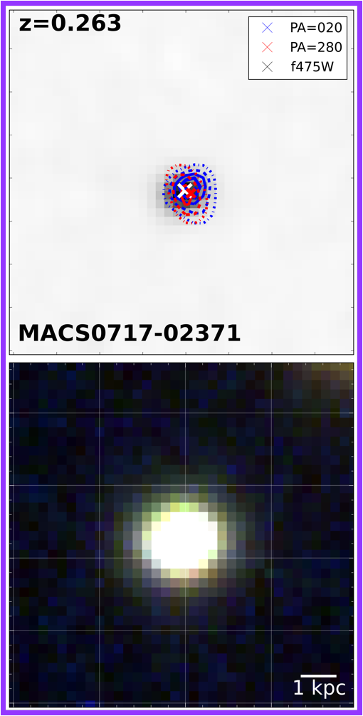
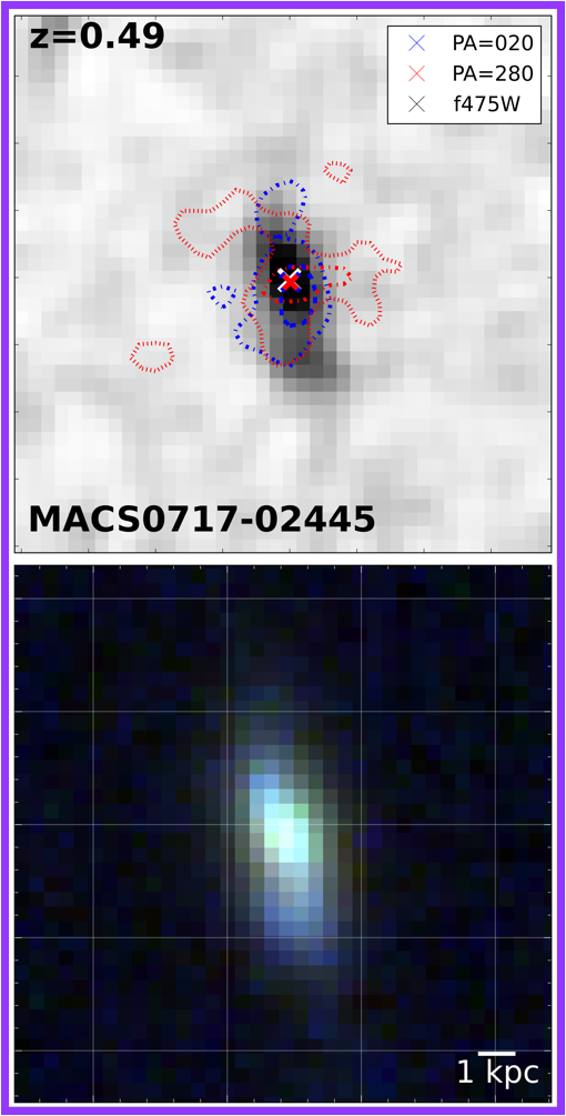
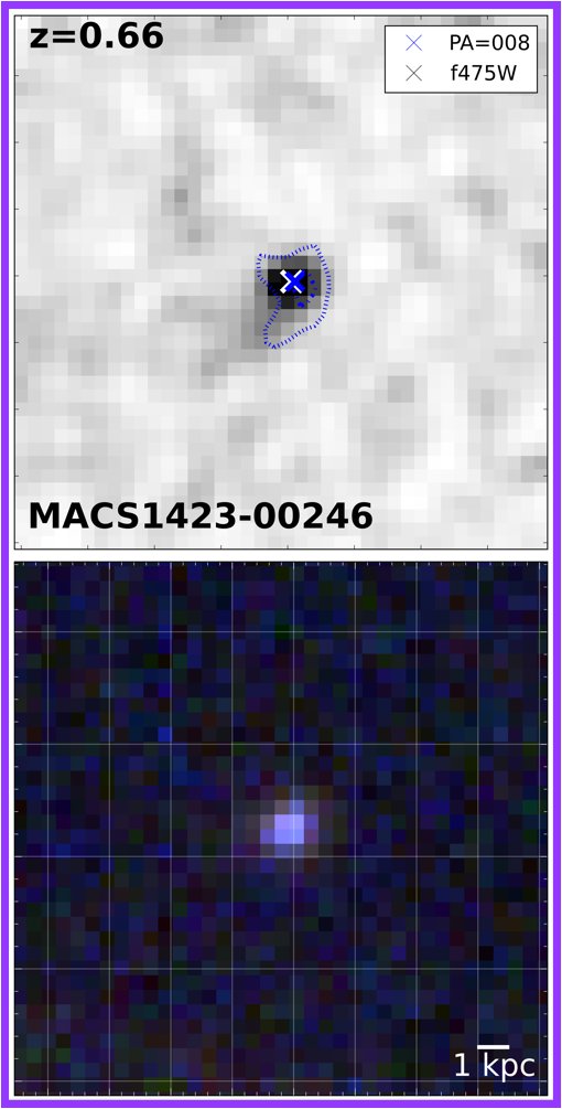
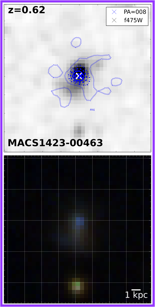
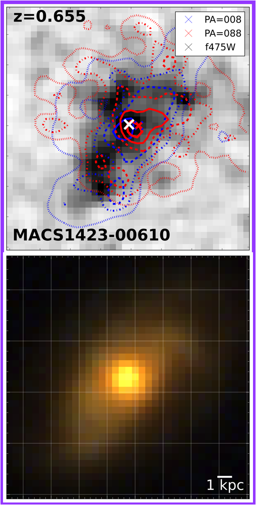
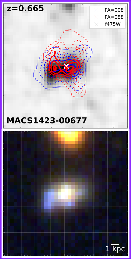
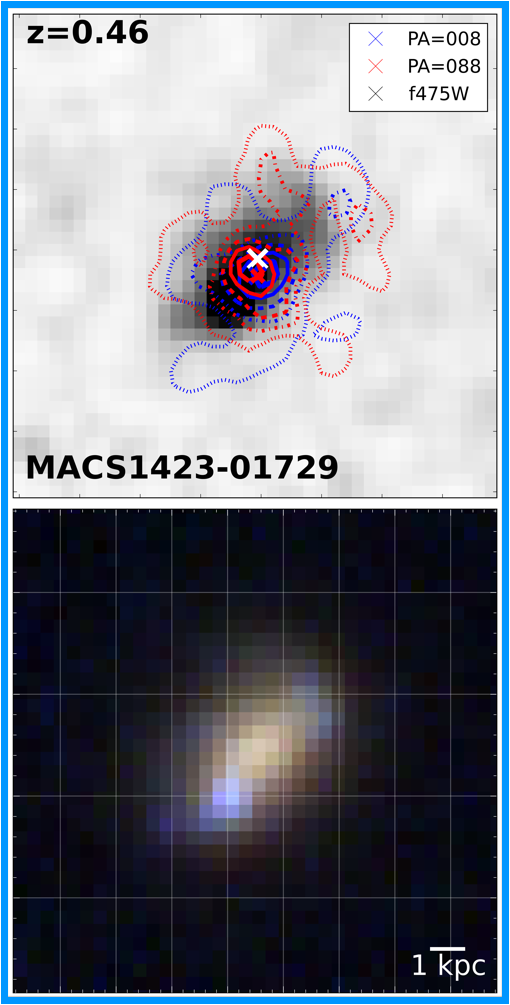
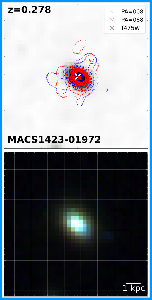
Figure 8.— Field galaxies with $\langle r($H$\alpha$ $)\rangle/\langle r(F745W)\rangle>1.2$. Panels, lines and colors are as in Fig. 5.

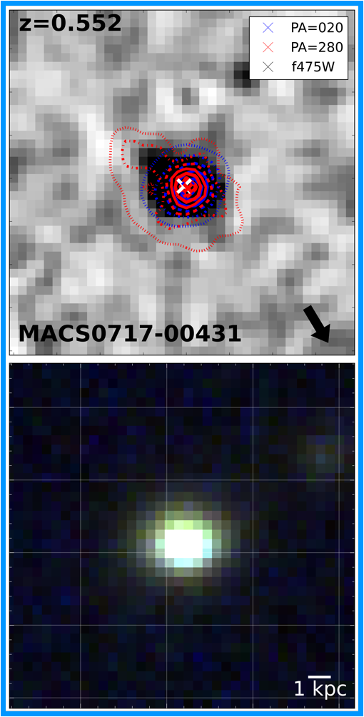
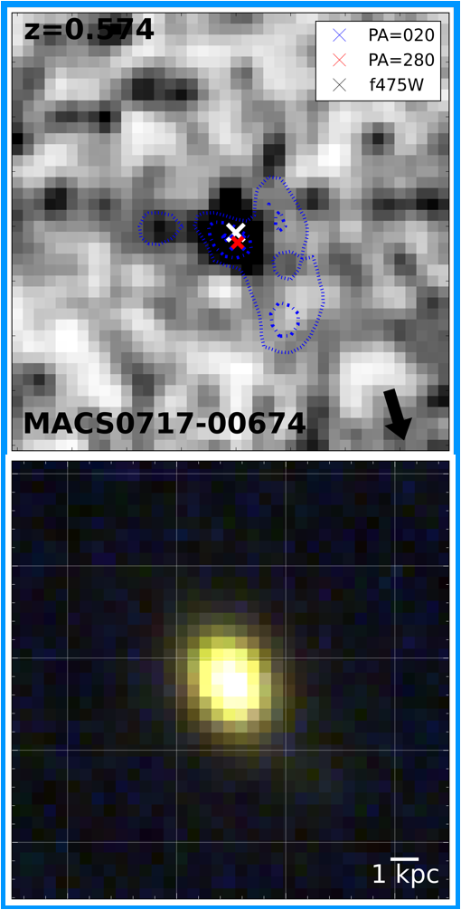
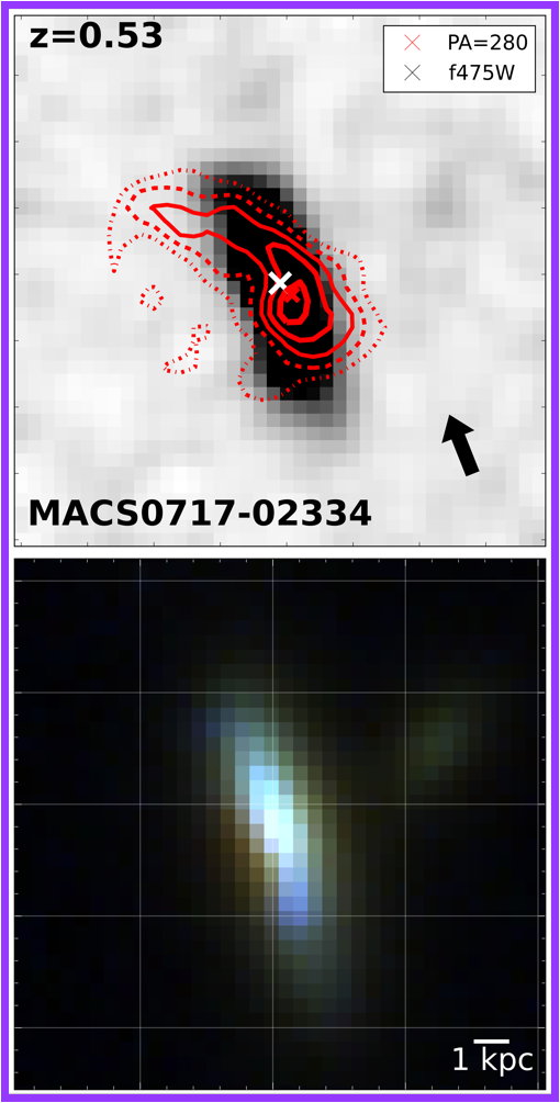
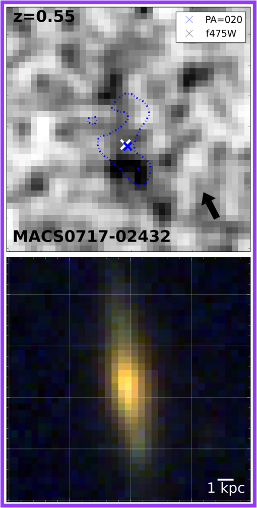
Figure 9.— Cluster galaxies with $\langle r($H$\alpha$ $)\rangle/\langle r(F745W)\rangle<0.8$. Panels, lines and colors are as in Fig. 5.

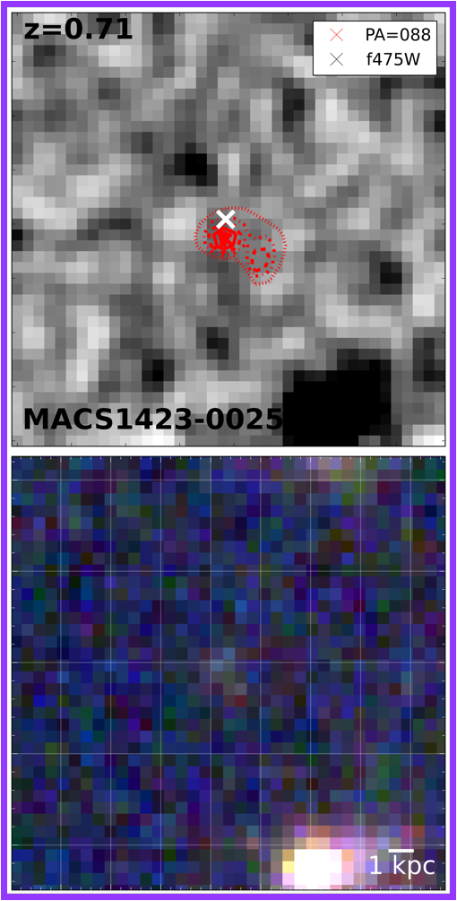
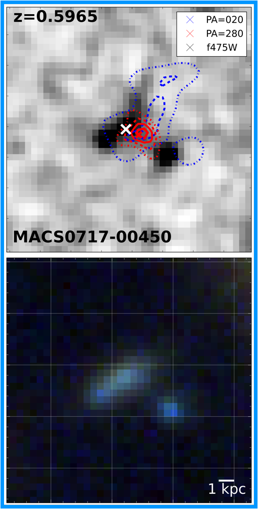
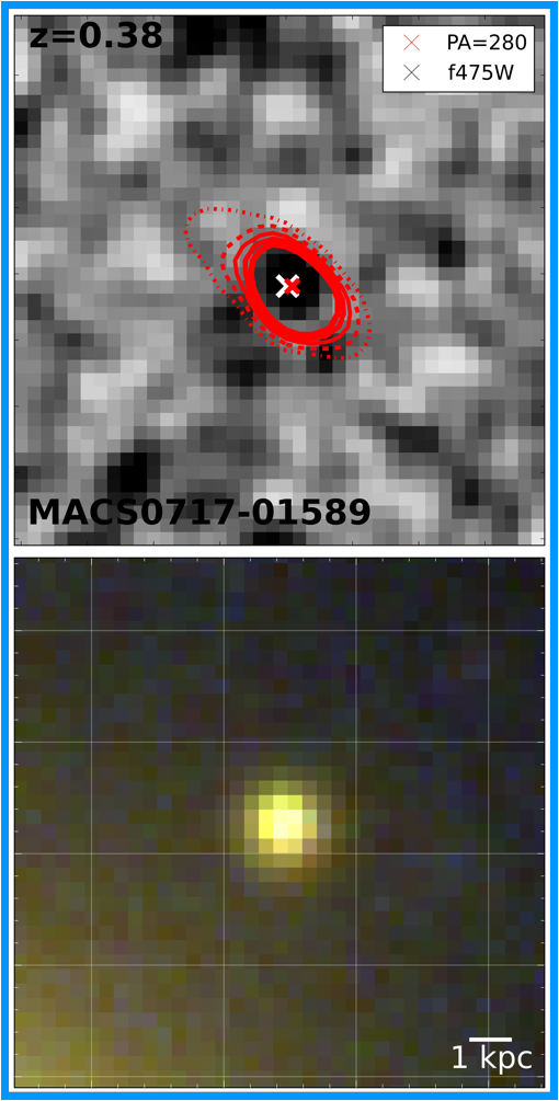
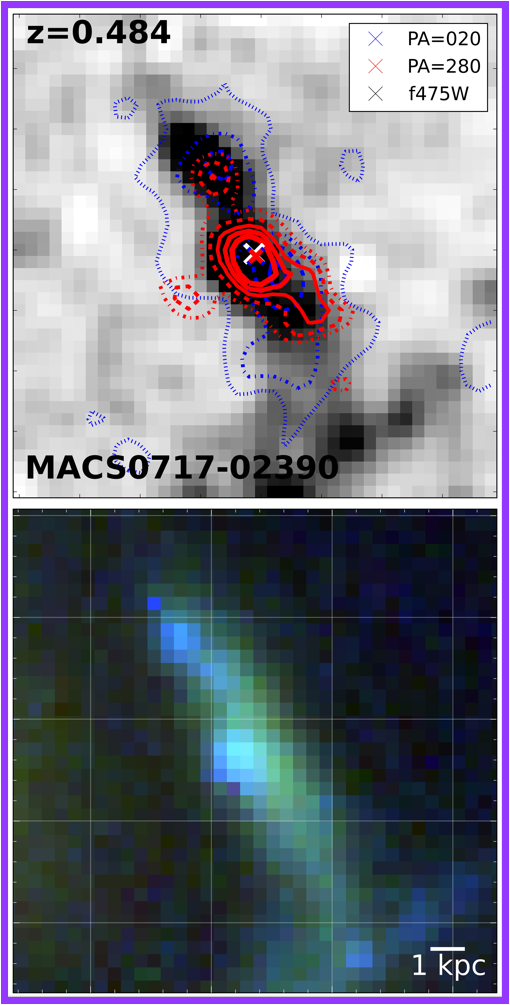
Figure 10.— Field galaxies with $\langle r($H$\alpha$ $)\rangle/\langle r(F745W)\rangle<0.8$. Panels, lines and colors are as in Fig. 5.

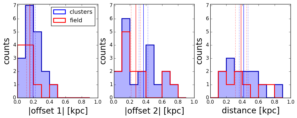
Figure 11.— Distribution of the offset of the H$\alpha$ emission with respect to the continuum. Left and central panel are the offsets in the two direction separately, right panel shows the combined offset, for the galaxies with both PAs. Vertical solid and dotted lines represent the means with errors. Most of the galaxies present an offset between the two emission. The displacement is slightly larger in clusters than in the field.

We group galaxies according to 1) the ratio of the average H$\alpha$ size to the average size of the rest-frame UV continuum shown in the top right panel of Fig. 4, and 2) the axis ratio of the continuum. The first classification scheme states whether the current star formation is occurring at larger or smaller radii than the recent star formation. We note that similar results are obtained when we consider the rest-frame optical continuum, which traces the older stars in the galaxy. The second is a rough attempt to describe the galaxy morphology in the light of the continuum. However, we note that all these classes of objects contain very heterogeneous cases with a variety of different features. It is therefore quite hard to perform a strict classification.

Figures 5-10 show the H$\alpha$ maps obtained as described in Section 3, for all galaxies in our sample. For each galaxy, also a color composite image of the galaxy based on the CLASH (Postman et al., 2012) HST data is shown. The blue channel is composed by the F435W, F475W, F555W, F606W, and F625W (the last one only for MACS0717) filters, the green by the F775W, F814W, F850lp, F105W, F110W filters, and the red by the F125W, F140W, F160W filters.

Figures 5 and 6 show the 6/25 cluster and 3/17 field galaxies with similar sizes in H$\alpha$ and in the rest-frame UV continuum ($0.8<\langle r($H$\alpha$ $)\rangle/\langle r(F745W)\rangle<1.2$). 4 cluster galaxies show elongated sizes in the light of the rest-frame UV continuum (axis ratio ¿1.2), while all field galaxies show symmetric shapes. Nonetheless, 3 galaxies in the field have clearly spiral morphologies.

Figures 7 and 8 show all galaxies with size of the H$\alpha$ light larger than the size measured from the continuum ($\langle r($H$\alpha$ $)\rangle/\langle r(F745W)\rangle>1.2$), in clusters and in the field respectively. The great majority of cluster and field galaxies fall into this class (15/25 and 10/17 respectively). Of these, 11 in clusters and 6 in the field show an elongated shape. Though being star forming, most of these galaxies show an early-type morphology in the color composite images. In clusters, this might be a sign of ongoing stripping.

Few galaxies have H$\alpha$ sizes smaller than continuum sizes ($\langle r($H$\alpha$ $)\rangle/\langle r(F745W)\rangle<0.8$) and are shown in Figures 9 and 10. In both environments, 2 out of 4 galaxies show symmetric profiles.

In general, our sample includes galaxies with a variety of morphologies and we find that there is no clear correlation between the extent of the H$\alpha$ emission and the galaxy color or morphology in the color images. This might suggest that there is no a unique mechanism responsible for extension of the H$\alpha$, but that different processes might be at work in galaxies of different types.

Overall, both in clusters and in the field 60% of galaxies show H$\alpha$ emission more extended than the emission in the rest-frame UV continuum. Half of the galaxies in the field show a symmetric shape, 35% in clusters.

When comparing the maps at different wavelengths, we also observe that the peak of the H$\alpha$ emission is displaced with respect to the F475W continuum emission. Figure 11 shows the distribution of the absolute value of the offsets in the two directions (obtained from the two different PAs) and, for the galaxies with both PAs, the real distance between the two peaks, obtained by combining the offsets. In both environments, the displacement is always smaller than 1 kpc. There is no a preferential direction of the offset. There are hints that galaxies in clusters are characterized by a marginally larger offset than field galaxies, but a larger number statistics will be needed to confirm the trends. The existence of the offset suggests that in most galaxies the bulk of the star formation is not occurring in the galaxy cores. Unsurprisingly given the small sample statistics, cluster and field means are compatible within the errors and a K-S test can not reject the hypothesis that the two distributions are drawn from the same parent distribution.

We note that in our analysis we have made the assumption that there is no spatial variation in extinction across the galaxy. Nonetheless, high-resolution imaging in multiple HST bands (Wuyts et al., 2012) as well as analysis of such data in combination with H$\alpha$ maps extracted from grism spectroscopy (Wuyts et al., 2013) indicate that such an assumption may be over-simplistic, particularly in the more massive galaxies where the largest spatial color variations are seen. It is hard to anticipate how corrections for non-uniform extinction might affect our conclusions, since the correction to the sizes will depend on the actual distribution of dust. For example, if dust is mostly in the centers (like a dust lane), it would make us overestimate the F475W sizes more than the H$\alpha$ sizes. Conversely, if dust is mostly in the outskirts the correction could lead us in the opposite direction. Reaching a firm conclusion would require obtaining Hb maps to trace the Balmer decrement. Unfortunately H_β is too blue for the G102 grism for these clusters.

4.2. Maps of H$\alpha$ and position within the clusters

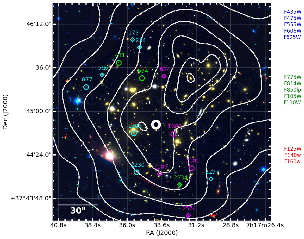
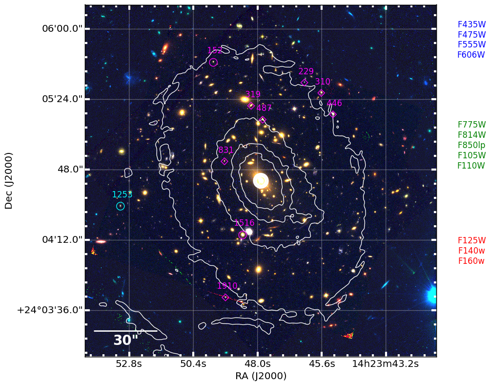
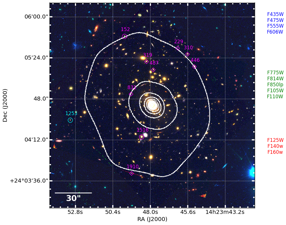
Figure 12.— Color composite image of MACS0717 (upper panels) and MACS1423 (bottom panels) based on the CLASH (Postman et al., 2012) HST data. The blue, green, and red channels are composed by the filters on the right. Galaxies with different size in H$\alpha$ and continuum are shown with different colors. Cyan: size(H$\alpha$)=size(continuum), magenta: size(H$\alpha$)¿size(continuum), green: size(H$\alpha$)¡size(continuum). Galaxies with different size ratios in the continuum are shown with different shapes. Diamonds: elongated continuum, circles: symmetric continuum. The white thick circle represents the cluster center. In the left panel, surface mass density contours are overplotted. A smoothing filter has been applied to the images for display purposes. Contours show $(0.5,1,1.5,2,5,10)\times 10^{10}\textrm{M}_{\odot}\,\textrm{kpc}^{-2}$. In right panel, X-ray emission is overplotted. Contours are spaced on a ”sqrt” scale from 0.0002 to 0.004 counts/s/px for MACS0717 and from 0.0005 to 0.2 counts/s/px for MACS1423.

For cluster galaxies, we can correlate their morphology with their location in the cluster, the surface mass density distribution and the X-ray emission, as shown in Fig. 12.

The mass maps were produced using SWUnited reconstruction code described in detail in Bradač et al. (2005) and Bradač et al. (2009). The method uses both strong and weak lensing mass reconstruction on a non-uniform adapted grid. From the set of potential values we determine all observables (and mass distribution) using derivatives. The potential is reconstructed by maximizing a log likelihood which uses image positions of multiply imaged sources, weak lensing ellipticities, and regularization as constraints. For both MACS1423 and MACS0717 we use CLASH data. In addition, for MACS0717 we make use of the arcs identified in HST archival imaging prior to Hubble Frontier Fields (Zitrin et al., 2009; Limousin et al., 2010) and spectroscopic redshifts obtained by Ma, Ebeling & Barrett (2009); Limousin et al. (2012); Ebeling, Ma & Barrett (2014). For MACS1423 we use spectroscopic redshifts and images identified in Limousin et al. (2010); and we add additional multiply imaged systems discovered by our team.

The X-ray images are based on Chandra data, and are described in Mantz et al. (2010) and von der Linden et al. (2014). For the contours shown in Fig.12, the images have been adaptively smoothed, after removing point sources identified in Ehlert et al. (2013).

In both clusters, galaxies are located within $\sim$0.4r₅₀₀ and do not seem to avoid the cluster cores, even though there might be possible projection effects. The two clusters present very different surface mass density distribution and X-ray emission: while MACS0717 extends along the north-west - south-east direction and has more than one main peak in the emissions, MACS1423 shows a symmetric surface mass density distribution and X-ray emission. We note that MACS1423 passes the very strict requirements on relaxedness defined in Mantz et al. (2014). In MACS0717 we find galaxies with both truncated or extended H$\alpha$ with respect to the rest-frame UV continuum, in MACS1423 all galaxies have H$\alpha$ light more extended than the continuum light. Despite the small number statistics, it appears that the truncated objects are only found between the merging clusters, suggesting that the spatial distribution of H$\alpha$ is indeed related to cluster dynamics: the most extreme cases of stripping are expected to take place in interacting systems (e.g., Owen et al., 2006; Smith et al., 2010; Owers et al., 2012).

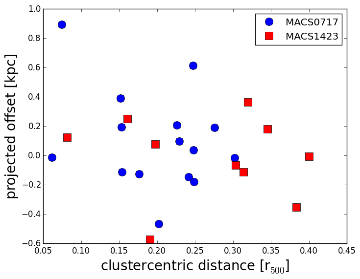
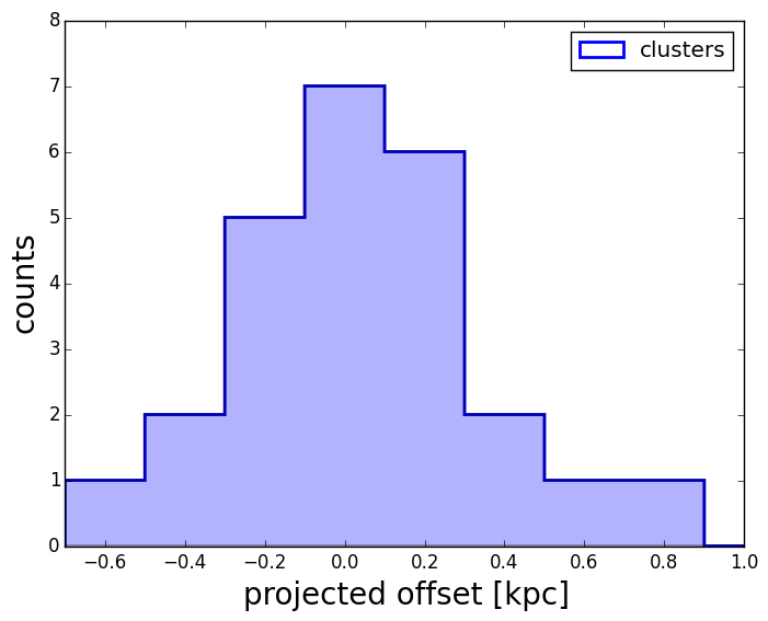
Figure 13.— Left: Projected offset along the cluster radial direction - distance from the cluster center relation for galaxies in clusters. Right: Projected offset along the line of sight distribution. No trends with distance are detected, indicating that the cluster center is not affecting the position of the peak of the H$\alpha$ emission.

Figure 13 quantifies the relation between the projected offset along the cluster radial direction and the distance of the galaxy from the cluster center, for cluster members. While most of the galaxies have a projected offset within $\pm$0.2 kpc, there are some galaxies with a larger offset. Almost half of the galaxies (55%) have a positive offset, the other half have a negative offset. No trends with distance are detected, indicating that the cluster center is not affecting the position of the peak of the H$\alpha$ emission. Galaxies with different H$\alpha$ extension are not clustered in particular regions of the clusters.

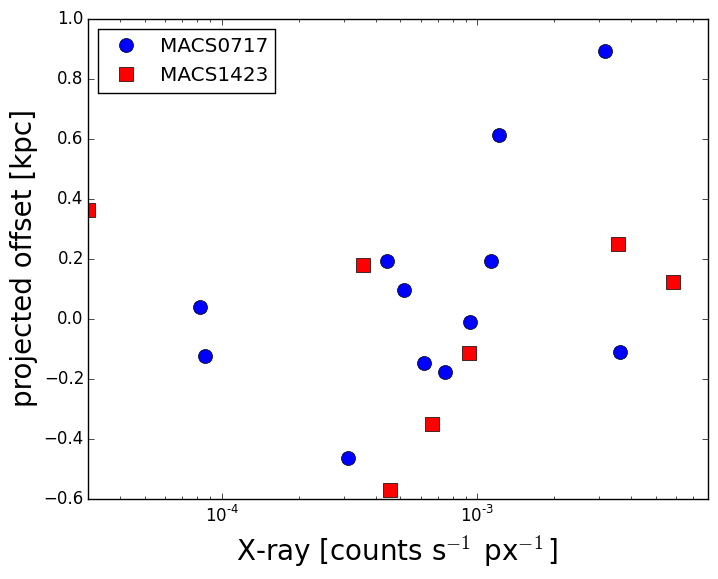
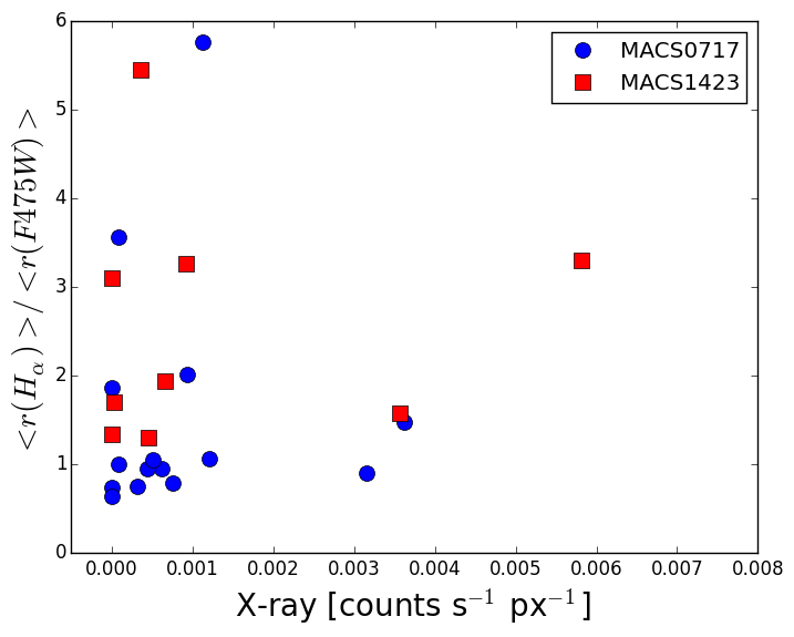
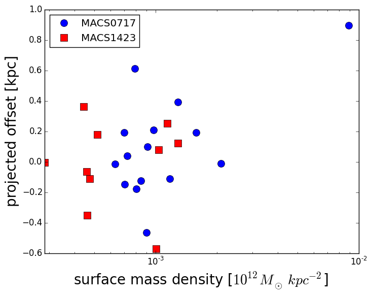
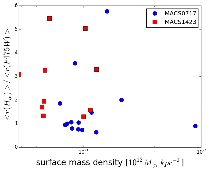
Figure 14.— Galaxy properties - cluster properties correlations. Upper row: X-ray emission, bottom row: Surface mass density. Left panels: projected offset along the line connecting the peak of the emission in the continuum and the cluster center. Right panels: ratio of r(H$\alpha$) to r(F745W). Shocks and strong gradients in the X-ray IGM might alter the relative position between the peak of the H$\alpha$ emission and the peak of the light of the of the young stellar population ($\sim$100 Myr), even though there is not statistically significant evidence to support this conclusion. Shocks and gradients do not alter the relative extension of the H$\alpha$ with respect to the continuum light.

There is increasing evidence for a correlation between the efficiency of the stripping phenomenon and the presence of shocks and strong gradients in the X-ray IGM (e.g., Owers et al., 2012; Vijayaraghavan & Ricker, 2013). Indeed, Figure 14 hints at potential correlations between the offset and X-ray emission or surface mass density. Similar results are obtained if we project the offset along the line that connects the galaxy to the peak of the X-ray emission. Nonetheless, Spearman rank-order correlation tests show that these trends are not statistically significant. Likewise, it seems that the extent of the H$\alpha$ size with respect to the continuum size does not strongly correlate with the X-ray emission nor the surface mass density, as confirmed by a Spearman rank-order correlation test.

Overall, it seems that shocks and strong gradients in the X-ray IGM might alter the relative position between the peak of the H$\alpha$ emission and the peak of the light of the recent star formation, even though we do not detect clear signs of gas compression and/or stripping.

We note that the lack of strong correlations does not allow us to identify a unique strong environmental effect that originates from the cluster center. We hypothesize that local effects, uncorrelated to the cluster-centric radius, play a larger role. Such effects weaken potential radial trends.

4.3. Notes on remarkable objects

In the following we describe some interesting objects presented in Figures 5-10.

Among galaxies with H$\alpha$ size similar to the rest-frame UV continuum size (Figures 5 and 6), we note that MACS0717-00236 is a spiral galaxy with three main peaks of H$\alpha$ emission. Indeed, the strongest emission comes from the two spiral arms, while the flux in the core of the galaxy is less important. A complex H$\alpha$ structure extends throughout the entire galaxy. Only one PA covers the entire galaxy, while the other misses one of the arms. In contrast, MACS0717-01477, even though showing a similar appearance in the color image to MACS0717-00236, is characterized by a much weaker and clumpy H$\alpha$ emission. MACS1423-01771 shows extended features both in the continuum and in the H$\alpha$ light.

Among galaxies with H$\alpha$ size larger than the continuum size (Figures 7 and 8), MACS0717-02189 and MACS0717-02574 show very elongated shapes in the continuum, but quite regular H$\alpha$ emission extended in both sizes. MACS1423-00229, MACS1423-01253 and MACS1423-01516 show very regular shapes in the continuum and very extended H$\alpha$ emission, in the case of MACS1423-01253 the emission is only in one direction. In MACS1423-00319 the H$\alpha$ emission is orthogonal to the continuum emission.

Finally, among galaxies with H$\alpha$ size smaller than the continuum size (Figures 9 and 10), MACS0717-02334 shows an H$\alpha$ emission which is bent with respect to the continuum. In this case, the truncated H$\alpha$ disk might be an example of ram pressure stripping, which removed the ISM. The orientation of the tail does not point away from the cluster center, but the bending might suggests that the galaxy formed from an infalling population experiencing the cluster environment for the first time (see, e.g., Smith et al., 2010).

It is also worth noting that MACS0717-01305 (Fig. 5) is very close to the cluster center, is located on a surface mass density distribution peak and is quite close to a peak in the X-ray emission. The shape of the H$\alpha$ emission seems to be unaffected by this peculiar position within the cluster, but the galaxy shows the largest projected offset along the line of sight.

4.4. Star Formation Rates

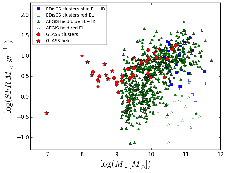
Figure 15.— GLASS cluster SFR-mass relation over plotted to the field relation at similar redshift (from Noeske et al., 2007) and the cluster relation at similar redshift (from Vulcani et al., 2010). Red filled circles: GLASS clusters; red filled stars: GLASS field. Blue squares: EDisCS clusters, green triangles: AEGIS field. Empty symbols: red galaxies with detected emission lines, filled symbols: blue galaxies with detected emission lines and galaxies detected at 24$\mu m$ (refer to Noeske et al., 2007; Vulcani et al., 2010, for details on the sample selection).

Figure 15 shows the SFR-mass plane for our cluster and field galaxies, together with that found by Noeske et al. (2007) for field galaxies at $z\sim 0.5$ and by Vulcani et al. (2010) for cluster galaxies also at $z\sim 0.5$. Our galaxies lay on the field SFR-mass relation of blue galaxies with emission lines or detected in the Infrared (see Noeske et al., 2007; Vulcani et al., 2010, for details on their sample selection), and even trace the upper limit. To some extent, this was expected having selected star forming cluster galaxies. This results, however, shows that at these redshifts cluster galaxies can be as star forming as field galaxies of similar mass. The location of our galaxies on the plane is also in line with what was found by Poggianti et al. (2015) for the local universe, who showed that galaxies with signs of ongoing stripping tend to be located above the best fit to the relation, indicating a SFR excess with respect to galaxies of the same mass but that are not being stripped. Recall that the field galaxies span a wide redshift range (0.2¡$z$¡0.7), therefore they lay on different regions of the SFR-mass plane simply due to the evolution of the SFR-M_∗ relation with $z$ (e.g., Noeske et al., 2007).

Both in clusters and in the field, the $\Sigma$SFR ranges from $\sim$0.1 to 1 $M_{\odot}\,\textrm{yr}^{-1}\,\textrm{kpc}^{-2}$, suggesting that the physical conditions in star forming galaxies do not strongly depend on environment.

5. Discussion and Conclusions

In this pilot study we have carried out an exploration of the spatial distribution of star formation in galaxies beyond the local universe, as traced by the H$\alpha$ emission in two of the GLASS clusters, MACS0717 and MACS1423. For this purpose, we have developed a new methodology to produce H$\alpha$ maps taking advantage of the WFC3-G102 data at two orthogonal PAs. We then visually selected galaxies with H$\alpha$ emission and, based on their redshift, assigned their membership to the cluster. We have used galaxies in the foreground and background of the two clusters to compile a field control sample. Both for field and cluster galaxies, we computed the extent of the emission and its position within the galaxy and compared these quantities to the younger stellar population as traced by the rest frame UV continuum (obtained by images in the F475W filter) and the older stellar population as traced by the rest-frame optical continuum (obtained by images in the F110W filter). We correlated galaxy properties to global and local cluster properties, in order to look for signs of cluster specific processes.

The main results of this analysis can be summarized as follows:

• Both in clusters and the field $\sim$60% of the galaxies are more extended in H$\alpha$ than in the rest-frame UV continuum. The emission appears larger in the cluster than in field galaxies. Trends are driven by a subpopulation ($\sim$20%) of cluster galaxies with H$\alpha$ emission at least three time as extended the continuum emission.

• Both in clusters and in the field there is an offset between the peak of the H$\alpha$ emission and that in the rest-frame UV continuum. The displacement can reach $\sim$1 kpc. In clusters the offset appears to be marginally larger.

• Comparing the extent of the offset and the cluster properties, we find a tentative correlation between the projected offset and both the X-ray emission and the mass surface density: the larger the emission, the bigger the offset between the emission in the rest-frame UV continuum and the emission in H$\alpha$. This offset seems to also to point at a cluster-specific mechanism.

• MACS0717 and MACS1423 present very different surface mass density distribution and X ray emission, indicating that MACS1423 is much more relaxed than MACS0717, which in contrast presents a double peak in the distribution. In MACS1423 all galaxies have H$\alpha$ disk larger than the rest-frame UV continuum, while in MACS0717 galaxies with both extend and truncated H$\alpha$ are observed. This finding suggests that gradients in the X-ray IGM might alter the relative position between the peak of the H$\alpha$ emission and the peak of the light of the young stellar population, even though at this stage correlations are not supported by statistical tests.

From our analysis a complex picture emerges and a simple explanation can not describe our observations. Even though galaxies in clusters and in the field present similar H$\alpha$ properties, the variety of their morphology suggests that they are at different stages of their evolution, therefore there can not be a unique mechanism acting on galaxies in the different environments. For example, the larger extension of H$\alpha$ with respect to the continuum seems to be a generic indication of inside-out growth (see also Nelson et al., 2012). Specific examples of this case include MACS1423-01253 and MACS1423-01910 in clusters (Fig.7) and MACS1423-01972 in the field (Fig.8). Investigating whether this growth is localized in a disk component will require careful bulge to disk decompositions which is planned for a future work. However, given the variety of morphologies, well-ordered disks do not appear to be the only site of star formation.

Furthermore, the larger average sizes in the cluster point to an additional cluster-specific mechanism responsible for stripping the ionized gas or perhaps for triggering additional star formation in the outskirts of the galaxies. The mechanism could be ram pressure stripping of the ionized gas or perhaps tidal compression of the outskirts or the galaxies, or both. Galaxies MACS0717-02189 and MACS1423-00446 (Fig.7) are examples of this possible mechanism.

Finally, in some cases, galaxies have been already deprived from their gas and are left with a smaller H$\alpha$ disk than the recent star formation. MACS0717-02334 (Fig.10) is a clear example of galaxies in such stage.

We note that the observed differences between cluster and field galaxies might be also due to the different mass and redshift distributions of the two samples, and not only to purely environmental effects.

The results from this pilot study illustrate the power and feasibility of space-based grism data to learn qualitatively new information about the mechanisms that regulate star formation in different environments during the second half of the life of the universe. Having developed the methods we are now in a position to carry out a larger scale investigation on the full GLASS cluster sample, when visual inspections and quality controls have been completed. The extended analysis will allow us not only to further distinguish and classify the processes acting in clusters from those acting on the field, but also to better correlate galaxy properties with the cluster global properties, investigating in detail the role of the environment in shutting down star formation.

References

- Atek et al. (2010) Atek, H. et al. 2010, The Astrophysical Journal, 723, 104.
- Balogh, Navarro & Morris (2000) Balogh, M. L., Navarro, J. F., and Morris, S. L. 2000, ApJ, 540, 113.
- Bell et al. (2004) Bell, E. F. et al. 2004, The Astrophysical Journal, 608, 752.
- Bell et al. (2007) Bell, E. F. et al. 2007, ApJ, 663, 834.
- Bertin & Arnouts (1996) Bertin, E. and Arnouts, S. 1996, Astronomy and Astrophysics Supplement, 117, 393.
- Bradač et al. (2005) Bradač, M. et al. 2005, A&A, 437, 39.
- Bradač et al. (2009) Bradač, M. et al. 2009, ApJ, 706, 1201.
- Brammer et al. (2014) Brammer, G. B. et al. 2014, STScI IRS.
- Brammer et al. (2012) Brammer, G. B. et al. 2012, The Astrophysical Journal Supplement, 200, 13.
- Bruzual & Charlot (2003) Bruzual, G. and Charlot, S. 2003, MNRAS, 344, 1000.
- Butcher & Oemler (1984) Butcher, H. and Oemler, Jr., A. 1984, ApJ, 285, 426.
- Capak et al. (2007) Capak, P. et al. 2007, ApJS, 172, 284.
- Castellano et al. (2014) Castellano, M. et al. 2014, A&A, 566, A19.
- Cooper et al. (2006) Cooper, M. C. et al. 2006, MNRAS, 370, 198.
- Cowie & Songaila (1977) Cowie, L. L. and Songaila, A. 1977, Nature, 266, 501.
- Daddi et al. (2007) Daddi, E. et al. 2007, ApJ, 670, 156.
- Dressler et al. (1997) Dressler, A. et al. 1997, ApJ, 490, 577.
- Dressler et al. (2013) Dressler, A. et al. 2013, ApJ, 770, 62.
- Dressler et al. (1999) Dressler, A. et al. 1999, ApJS, 122, 51.
- Ebeling, Ma & Barrett (2014) Ebeling, H., Ma, C.-J., and Barrett, E. 2014, ApJS, 211, 21.
- Ehlert et al. (2013) Ehlert, S. et al. 2013, MNRAS, 428, 3509.
- Fasano et al. (2000) Fasano, G. et al. 2000, ApJ, 542, 673.
- Finn et al. (2005) Finn, R. A. et al. 2005, ApJ, 630, 206.
- Fontana et al. (2004) Fontana, A. et al. 2004, A&A, 424, 23.
- Fontana et al. (2006) Fontana, A. et al. 2006, A&A, 459, 745.
- Fumagalli et al. (2014) Fumagalli, M. et al. 2014, MNRAS, 445, 4335.
- Geach et al. (2008) Geach, J. E. et al. 2008, MNRAS, 388, 1473.
- Gonzaga et al. (2012) Gonzaga, S. et al. 2012.
- Guglielmo et al. (2015) Guglielmo, V. et al. 2015, MNRAS, 450, 2749.
- Gunn & Gott (1972) Gunn, J. E. and Gott, III, J. R. 1972, ApJ, 176, 1.
- Hatch et al. (2011) Hatch, N. A. et al. 2011, MNRAS, 415, 2993.
- Hopkins & Beacom (2006) Hopkins, A. M. and Beacom, J. F. 2006, ApJ, 651, 142.
- Hopkins et al. (2001) Hopkins, A. M. et al. 2001, AJ, 122, 288.
- James et al. (2005) James, P. A. et al. 2005, A&A, 429, 851.
- Karim et al. (2011) Karim, A. et al. 2011, The Astrophysical Journal, 730, 61.
- Kennicutt (1998) Kennicutt, R. C. 1998, Astrophysical Journal v.498, 498, 541.
- Kennicutt, Tamblyn & Congdon (1994) Kennicutt, R. C., Tamblyn, P., and Congdon, C. E. 1994, Astrophysical Journal, 435, 22.
- Kodama et al. (2004) Kodama, T. et al. 2004, MNRAS, 354, 1103.
- Koekemoer et al. (2003) Koekemoer, A. M. et al. 2003, The 2002 HST Calibration Workshop : Hubble after the Installation of the ACS and the NICMOS Cooling System, 337.
- Koyama et al. (2011) Koyama, Y. et al. 2011, ApJ, 734, 66.
- Koyama et al. (2013) Koyama, Y. et al. 2013, MNRAS, 428, 1551.
- Kroupa (2001) Kroupa, P. 2001, MNRAS, 322, 231.
- Kurk et al. (2004) Kurk, J. D. et al. 2004a, A&A, 428, 817.
- Kurk et al. (2004) Kurk, J. D. et al. 2004b, A&A, 428, 793.
- Larson, Tinsley & Caldwell (1980) Larson, R. B., Tinsley, B. M., and Caldwell, C. N. 1980, ApJ, 237, 692.
- Limousin et al. (2010) Limousin, M. et al. 2010, MNRAS, 405, 777.
- Limousin et al. (2012) Limousin, M. et al. 2012, A&A, 544, A71.
- Ma, Ebeling & Barrett (2009) Ma, C.-J., Ebeling, H., and Barrett, E. 2009, ApJ, 693, L56.
- Madau & Dickinson (2014) Madau, P. and Dickinson, M. 2014, eprint arXiv, 1403, 7.
- Madau, Pozzetti & Dickinson (1998) Madau, P., Pozzetti, L., and Dickinson, M. 1998, ApJ, 498, 106.
- Mantz et al. (2010) Mantz, A. et al. 2010, MNRAS, 406, 1773.
- Mantz et al. (2014) Mantz, A. B. et al. 2014, MNRAS, 440, 2077.
- Merluzzi et al. (2013) Merluzzi, P. et al. 2013, MNRAS, 429, 1747.
- Moore et al. (1996) Moore, B. et al. 1996, Nature, 379, 613.
- Nelson et al. (2012) Nelson, E. J. et al. 2012, The Astrophysical Journal Letters, 747, L28.
- Nelson et al. (2015) Nelson, E. J. et al. 2015, ArXiv e-prints.
- Nelson et al. (2013) Nelson, E. J. et al. 2013, The Astrophysical Journal Letters, 763, L16.
- Noeske et al. (2007) Noeske, K. G. et al. 2007, ApJ, 660, L43.
- Nulsen (1982) Nulsen, P. E. J. 1982, MNRAS, 198, 1007.
- Oesch et al. (2010) Oesch, P. A. et al. 2010, The Astrophysical Journal Letters, 709, L16.
- Owen et al. (2006) Owen, F. N. et al. 2006, AJ, 131, 1974.
- Owers et al. (2012) Owers, M. S. et al. 2012, ApJ, 750, L23.
- Peng et al. (2010) Peng, Y.-j. et al. 2010, ApJ, 721, 193.
- Poggianti et al. (2009) Poggianti, B. M. et al. 2009, ApJ, 697, L137.
- Poggianti et al. (2015) Poggianti, B. M. et al. 2015, ArXiv e-prints.
- Poggianti et al. (1999) Poggianti, B. M. et al. 1999, ApJ, 518, 576.
- Poggianti et al. (2006) Poggianti, B. M. et al. 2006, ApJ, 642, 188.
- Postman et al. (2012) Postman, M. et al. 2012, ApJS, 199, 25.
- Salpeter (1955) Salpeter, E. E. 1955, ApJ, 121, 161.
- Santini et al. (2015) Santini, P. et al. 2015, ApJ, 801, 97.
- Schmidt et al. (2013) Schmidt, K. B. et al. 2013, MNRAS, 432, 285.
- Schmidt et al. (2014) Schmidt, K. B. et al. 2014, ApJ, 782, L36.
- Smith et al. (2010) Smith, R. J. et al. 2010, MNRAS, 408, 1417.
- Sobral et al. (2013) Sobral, D. et al. 2013, MNRAS, 428, 1128.
- Straughn et al. (2011) Straughn, A. N. et al. 2011, The Astronomical Journal, 141, 14.
- Treu et al. (2003) Treu, T. et al. 2003, ApJ, 591, 53.
- Treu et al. (2015) Treu, T. et al. 2015, ApJ submitted.
- van Dokkum et al. (2011) van Dokkum, P. G. et al. 2011, ApJ, 743, L15.
- Vijayaraghavan & Ricker (2013) Vijayaraghavan, R. and Ricker, P. M. 2013, MNRAS, 435, 2713.
- von der Linden et al. (2014) von der Linden, A. et al. 2014, MNRAS, 439, 2.
- Vulcani et al. (2010) Vulcani, B. et al. 2010, ApJ, 710, L1.
- Wuyts et al. (2012) Wuyts, S. et al. 2012, ApJ, 753, 114.
- Wuyts et al. (2013) Wuyts, S. et al. 2013, ApJ, 779, 135.
- Yagi et al. (2015) Yagi, M. et al. 2015, AJ, 149, 36.
- Zitrin et al. (2009) Zitrin, A. et al. 2009, ApJ, 707, L102.