Regular black holes in $f(R)$ gravity coupled to nonlinear electrodynamics

Abstract

We obtain a class of regular black hole solutions in four-dimensional $f(R)$ gravity, $R$ being the curvature scalar, coupled to a nonlinear electromagnetic source. The metric formalism is used and static spherically symmetric spacetimes are assumed. The resulting $f(R)$ and nonlinear electrodynamics functions are characterized by a one-parameter family of solutions which are generalizations of known regular black holes in general relativity coupled to nonlinear electrodynamics. The related regular black holes of general relativity are recovered when the free parameter vanishes, in which case one has $f(R)\propto R$. We analyze the regularity of the solutions and also show that there are particular solutions that violate only the strong energy condition

I Introduction

The theory of general relativity (GR) has passed many experimental and observational tests and is widely accepted as the best theory of gravitation. Even with such a success, there are some aspects in GR to be better understood. In this sense, the prediction of spacetime singularities and the difficulty to be quantized through standard methods are two important issues to be mentioned. The singularity problem is connected to the existence of black holes, which are probably the most intriguing objects predicted by GR. In the simplest case, the Schwarzschild black hole, the spacetime presents an event horizon which hides a curvature singularity inside of it. More generally, if the matter-energy content of the spacetime satisfies some reasonable physical conditions, the so-called energy conditions, the singularity theorems of GR sing-theo assure that the singularity is inevitable. Even though the singularity can be hidden by the presence of an event horizon, which protects the exterior world, its own presence signals the breakdown of the physical laws. In other words, a good physical theory should be free of singularities. It is believed that a complete theory of quantum gravity would have such a good property, but such a theory does not exist yet. Hence, while a theory of quantum gravity is not formulated, good strategies to get rid of singularities is to search for alternative matter-field models within GR, and to search for alternative theories of gravity that are free of singularities.

Within GR, singularities can be avoided if the energy conditions assumed by the singularity theorems are somehow violated. In the case of black holes, the singularity can be replaced by a regular region filled by some kind of matter or field that violates at least the strong energy condition. In fact, the matter content of the first regular black hole solution found in GR is such that, near the center, it satisfies a de Sitter type equation of state $p=-\rho$, with $\rho$ and $p$ being the energy density and the pressure of an effective perfect fluid model representing the energy-momentum tensor of the Bardeen black hole Bardeen . It clearly violates the strong energy condition. As a matter of fact, a perfect fluid satisfying a de Sitter equation of state has long been suggested to solve the cosmological singularity problem sakharov-gliner . A wide class of regular black holes solutions found in the literature follows this idea, the singularity being replaced by a regular distribution of matter satisfying a de Sitter type equation of state at least at the central core. The class of solutions that followed Bardeen’s idea evolved towards models whose source is the energy-momentum coming from some kind of nonlinear electromagnetic theory (see, e.g., ABG-ned , see reviewRBH for a review). A second very interesting class of regular black holes followed precisely the idea of modeling the matter content by a perfect fluid obeying the relation $p=-\rho$ (see, e.g., dym-deSitter ).

The singularity problem in GR is linked to the important observational result that the Universe is in a phase of accelerated expansion, as first inferred from type Ia supernovae data SNIa and confirmed by several other tests (see, e.g., accel for reviews). Considering a Friedman-Lamaître-Robertson-Walker cosmological spacetime fulfilled by a perfect fluid, in order to have an accelerated expansion, Einstein equations require the perfect fluid to satisfy the condition $\rho+3p<0$, where $\rho$ and $p$ are respectively the energy density and pressure of the fluid. More than that, in the cosmic concordance model, namely, the $\Lambda$CDM model, the perfect fluid model for the dark energy satisfies $p=-\rho$. Assuming an equation of state in the form $p=\omega\rho$, several cosmological tests indicate that the present accelerated phase of the Universe requires $\omega\lesssim-1$ lima . These facts motivated more studies on regular black holes modeled by de Sitter like and phantom matter fields deSitter2-phantom (see also dym-deSitter ).

Beyond GR there are many proposals of alternative theories of gravity. Besides trying to solve the singularity problem and to avoid introducing matter with nonstandard physical properties, alternative theories have been proposed to account for quantum corrections in the action. A well established proposal is the $f(R)$ gravity fR ; deFelice which replaces the Einstein-Hilbert Lagrangian density by a general function of the Ricci scalar $R$. The already mentioned issue of an accelerated cosmological expansion phase motivated also several other proposals which are still being developed. Worth of mentioning are the $f(R,\Theta)$ fRT , the $f(G)$ fG , the $f(R,G)$ fRG , and the $f(R,\Theta,R_{\mu\nu}\Theta^{\mu\nu})$ odintsov gravity theories. In this notation, $G$ stands for the Gauss-Bonnet term, $\Theta^{\mu\nu}$ and $\Theta$ represent the energy-momentum tensor and its trace, respectively, and $R^{\mu\nu}$ is the Ricci tensor. There are many applications of such generalized $f(R)$ gravity theories in cosmological models (see the reviews of Refs. fR ; deFelice , see also fR-cosmol ). Similarly, in the context of the Teleparallel Theory of gravity (TTG) TT there are also analogous models that modify the standard TTG into more general theories. The $f(T)$ theory is the analogous of the $f(R)$ gravity whose modification was introduced to try to account for the same problems of GR (see fT for a list of references). Further generalizations are the $f(T,\Theta)$ fTTc , the $f(T,T_{G})$ fTTG , and the $f(\mathcal{T})$ gravity theories ednaldo . For a review on the applications of modified theories of gravity see, e.g., Ref. bamba (see also fT-cosmol ).

On the other side, considering matter and fields models, the Maxwell electromagnetism is also a very well established theory that has passed all the experimental tests. But, with the aim of avoiding divergent terms in quantum electrodynamics, Born and Infeld BI proposed a modified version of the Maxwell theory which, together with other generalizations, is dubbed the nonlinear electrodynamics (NED) peres . When coupled to GR, the NED theory produces regular black hole solutions where the singularity is avoided by a regular distribution of the (new) electromagnetic field that fulfills the central core of the black hole. In fact, construction of regular solutions of GR coupled to NED has been largely studied in the literature NED . This fact motivates the construction of regular black hole solutions in the new (generalized) gravity theories coupled to the generalized models for matter fields, since it is a natural way to investigate the properties of the new theories in the strong field regime.

Within $f(R)$ gravity theories many black hole solutions are found in the literature, either using the metric formalism metricfR or the Palatini formalism PalatinifR . Yet, in order to find regular black hole solutions, special kinds of matter are needed. For instance, nonlinear electromagnetic and Yang-Mills fields are considered as sources to build regular $f(R)$ gravity black holes. In other cases, including electric charge, the matter distribution must satisfy particular conditions, generating a wormhole type structure avoiding thus the central singularity.

Motivated by the scenario summarized above, in the present work we follow the idea of coupling a nonlinear electrodynamics (NED) to the chosen (new) gravity theory, and establishing a method to find exact solutions in such a way to be able to built regular black hole solutions within such a theory.

The paper is structured as follows. In Sec. II the basic equations for the $f(R)$ theory minimally coupled to a general electromagnetic action are presented, a spherically symmetric static metric is chosen and the explicit field equations for the metric functions and electromagnetic field are given in terms of a Schwarzschild radial coordinate $r$. Section III is devoted to present new regular black holes solutions, it is divided into four subsections. In the first subsection, III.1, after making a simplifying hypothesis, the only relevant metric coefficient is written in terms of a generic mass function $M(r)$. Function $f_{R}$, that is the derivative of $f(R)$ with respect to $R$, is integrated resulting in a linear function of the radial coordinate. All the relevant equations are then written in terms of $M(r)$ and the energy conditions are written explicitly in terms of the effective energy-momentum tensor of the theory. In subsection III.2, we show that the ansatz for $M(r)$ reproduces the Reissner-Nordström black hole solution in the particular case where $f_{R}=1$, verifying the consistency of the procedure used to generate the exact solutions. Subsection III.3 is reserved to present a solution which has two horizons and is regular throughout the spacetime. A particular form of $M(r)$ is chosen in order to produce regular black holes, as known from previous works. The solution is new in the sense that it is the first of this class within $f(R)$ gravity coupled to NED theories. The solution is analyzed in some detail and it is shown that the weak energy condition is violated in the central region of the spacetime inside the event horizon. A careful analysis of the regularity and asymptotic behavior of this solution is performed in Sec. A.1 of Appendix A. In subsection III.4, a second solution representing a regular black hole in $f(R)$ coupled to NED theory is presented and analyzed. In this case, only the strong energy condition is violated inside the event horizon. The regularity of the solution at the asymptotic limit (spatial infinity) of this solution is considered in Sec. A.2 of Appendix A. In Sec. IV we make final remarks and conclude.

II The equations of motion in $f(R)$ gravity

The $f(R)$ gravity is a generalization of GR which in the metric formalism is obtained from the action (we follow the sign conventions of Ref. deFelice ).

$$S_{f(R)}=\int d^{4}x\sqrt{-g}\left[f(R)+2\kappa^{2}\mathcal{L}_{m}\right],$$ (1)

where $g$ stands for the determinant of the metric $g_{\mu\nu}$, $f(R)$ is a given function of the Ricci scalar $R$, $\mathcal{L}_{m}$ represents the Lagrangian density of the matter and other fields, and $\kappa^{2}=8\pi G/c^{4}$, with $G$ and $c$ being the Newton’s gravitational constant and the speed of light, respectively (from now on we choose units such that $G=1$ and $c=1$). Varying action (1) with respect to the metric it results

$$f_{R}R^{\mu}_{\;\;\nu}-\frac{1}{2}\delta^{\mu}_{\nu}f+\left(\delta^{\mu}_{\nu}\square-g^{\mu\beta}\nabla_{\beta}\nabla_{\nu}\right)f_{R}=\kappa^{2}\Theta^{\mu}_{\;\;\nu}\;,$$ (2)

where $f_{R}\equiv df(R)/dR$, $R^{\mu}_{\;\;\nu}$ is the Ricci tensor, $\nabla_{\nu}$ stands for the (metric compatible) covariant derivative, $\square\equiv g^{\alpha\beta}\nabla_{\alpha}\nabla_{\beta}$ is the d’Alembertian, and $\Theta_{\mu\nu}$ is the matter energy-momentum tensor.

In the present work we consider a nonlinear electrodynamics (NED) model coupled to the $f(R)$ gravity, so that the Lagrangian density for the matter fields in the action (1) may be particularized as $\mathcal{L}_{m}\equiv\mathcal{L}_{NED}(F)$, where $F=(1/4)F^{\mu\nu}F_{\mu\nu}$, and with $F_{\mu\nu}$ being the Faraday-Maxwell tensor (here we neglect the electromagnetic sources). In such a case, the energy-momentum tensor is written as

$$\Theta^{\mu}_{\;\;\nu}=\delta^{\mu}_{\nu}\mathcal{L}_{NED}-\frac{\partial\mathcal{L}_{NED}(F)}{\partial F}F^{\mu\alpha}F_{\nu\alpha}\;.$$ (3)

The canonical energy-momentum tensor of the Maxwell theory follows in the particular case where $\mathcal{L}_{NED}\equiv F$.

The Faraday-Maxwell tensor may be given in terms of a gauge potential in the usual form $F_{\mu\nu}=\partial_{\mu}A_{\nu}-\partial_{\nu}A_{\mu}$. Then, varying action (1) with respect to the potential $A_{\mu}$ one gets a generalized version of the Maxwell equations

$$\nabla_{\mu}\left[F^{\mu\nu}\mathcal{L}_{F}\right]\equiv\partial_{\mu}\left[\sqrt{-g}F^{\mu\nu}\mathcal{L}_{F}\right]=0\;,$$ (4)

where $\mathcal{L}_{F}=\partial\mathcal{L}_{NED}/\partial F$.

Furthermore, taking the trace of Eq. (2) one gets

$$f_{R}R-2f+3\square f_{R}=\kappa^{2}\Theta\,,$$ (5)

where $\Theta\equiv g^{\mu\nu}\Theta_{\mu\nu}=4\mathcal{L}_{NED}-F\mathcal{L}_{F}$.

We then consider a spherically symmetric and static spacetime, whose line element, in Schwarzschild-like coordinates, reads

$$ds^{2}=e^{a(r)}dt^{2}-e^{b(r)}dr^{2}-r^{2}\left[d\theta^{2}+\sin^{2}\theta d\phi^{2}\right]\;,$$ (6)

where $a(r)$ and $b(r)$ are arbitrary functions of the radial coordinate $r$ alone. With this, the electromagnetic source is the electric charge only, and the magnetic parts of the Faraday-Maxwell tensor $F_{\mu\nu}$ vanish identically. Moreover, due to the symmetry the only nonzero component is electric intensity $F^{10}(r)$ wainwright . Hence, we can integrate the resulting equation from (4) for $\nu=0$ to get,

$$F^{10}(r)=\frac{q}{r^{2}}e^{-\left(a(r)+b(r)\right)/2}\mathcal{L}_{F}^{-1}(r)\;,$$ (7)

where $q$ is an integration constant representing the electric charge of the source.

The equations of motion for the $f(R)$ gravity coupled to a NED are then found by using the line element (6), the Faraday-Maxwell tensor (7), the energy-momentum (3), and the equations of motion (2),

$$\frac{e^{-b}}{4r}\Big{\{}4r\frac{d^{2}f_{R}}{dr^{2}}+2\left[4-rb^{\prime}\right]\frac{df_{R}}{dr}+\big{[}ra^{\prime}b^{\prime}-2ra^{\prime\prime}-r(a^{\prime})^{2}-4a^{\prime}\big{]}f_{R}+2re^{b}f\Big{\}}$$

$$\qquad=-\kappa^{2}\left[\mathcal{L}_{NED}+\frac{q^{2}}{r^{4}}\mathcal{L}_{F}^{-1}\right],$$ (8)

$$\frac{e^{-b}}{4r}\Big{\{}2\left[4+ra^{\prime}\right]\frac{df_{R}}{dr}+\left[(4+ra^{\prime})b^{\prime}-2ra^{\prime\prime}-r(a^{\prime})^{2}\right]f_{R}+2re^{b}f\Big{\}}$$

$$\qquad=-\kappa^{2}\left[\mathcal{L}_{NED}+\frac{q^{2}}{r^{4}}\mathcal{L}_{F}^{-1}\right],$$ (9)

$$\frac{e^{-b}}{2r^{2}}\Big{\{}2r^{2}\frac{d^{2}f_{R}}{dr^{2}}+[r^{2}(a^{\prime}-b^{\prime})+2r]\frac{df_{R}}{dr}+[r(b^{\prime}-a^{\prime})+2(e^{b}-1)]f_{R}+r^{2}e^{b}f\Big{\}}$$

$$\qquad=-\kappa^{2}\mathcal{L}_{NED},$$ (10)

where the prime (^′) stands for the total derivative with respect to the radial coordinate $r$.

To be complete, we stress that Eq. (5) is satisfied by any solution of Eqs. (8)-(10). This can be shown explicitly by combining these three equations and noticing that the Ricci scalar for the present case is given by

$$R=e^{-b}\left[a^{\prime\prime}+\left(a^{\prime}-b^{\prime}\right)\left(\frac{a^{\prime}}{2}+\frac{2}{r}\right)+\frac{2}{r^{2}}\right]-\frac{2}{r^{2}}\;.$$ (11)

In the next section we shall solve of Eqs. (8)-(10) and present the first solutions of regular black holes in the $f(R)$ gravity coupled to a nonlinear electrodynamics theory.

III New regular black hole solutions

III.1 Simplifying hypothesis and the ansatz for the mass function

Once the spacetime geometry is assumed to be static and to carry the spherical symmetry, all the metric function and fields depend on the radial coordinate only and then the system of differential equations may be further simplified by making suitable hypotheses. Now, by subtracting Eq. (9) from Eq. (8) it results

$$\frac{e^{-b}}{2r}\left[2r\frac{d^{2}f_{R}}{dr^{2}}-\left(r\frac{df_{R}}{dr}+2f_{R}\right)\left(a^{\prime}+b^{\prime}\right)\right]=0.$$ (12)

This is a second-order ordinary differential equation for $f_{R}$, whose general solution can be found once functions $a(r)$ and $b(r)$ are known. However, these two function are found in general just by solving the complete nonlinear system of coupled equations resulting from Eqs. (8), (9), and (10) after specifying the NED Lagrangian. Since we are interested in black hole solutions, the usual strategy at this point is to make an ansatz that leads to that kind of solutions. An interesting choice is to fix the following relation

$$b(r)=-a(r).$$ (13)

Such a relation is a consequence of the field equations in GR, but that is not the case in $f(R)$ gravity theories, where such a choice represents a further constraint on the possible solutions. By fixing the metric coefficients as given in (13), equation (12) becomes

$$e^{-b(r)}\frac{d^{2}f_{R}}{dr^{2}}=0\;.$$ (14)

The general solution of such an equation, for $e^{-b(r)}\neq 0$, is given by the expression

$$f_{R}(r)=c_{1}r+c_{0}\,,$$ (15)

where $c_{1}$ and $c_{0}$ are integration constants. Within the class of spherically symmetric systems, this approach has recurrently been used to find new solution of $f(R)$ gravity theories (see, e.g., Eq. (12) of cognola and Eq. (15) of sebastiani ). Here it is then seen that the solution (15) leads to a simple generalization of GR theory. In the case with $c_{1}=0$ and $c_{0}=1$, we recover GR, since the integration of Eq. (15) would furnish $f(R)=R$. On the other hand, in the general case when $c_{1},c_{0}\,\neq 0$ and once the function $a(r)$ and $b(r)$ are given, Eq. (11) can be inverted to write $r$ as a function of $R$, $r\equiv r(R)$, and finally the integration of (15) yields

$$f(R)=c_{0}R+c_{1}\int r(R)dR,$$ (16)

where we have set an integration constant to zero. From Eq. (16) it is clearly seen that the second term is the responsible for the contributions to the $f(R)$ gravity beyond the standard GR, including possibly nonlinear terms on the Ricci scalar $R$.

The linear dependence of $f_{R}$ on $r$ in Eq. (15) implies it is an unbounded function at the asymptotic limit $r\rightarrow+\infty$. However, as we show explicitly in Appendix A, for the particular solutions presented in this work, such an unbounded value implies no divergence in any of the physical and geometric quantities of the corresponding spacetimes. In fact, all the equations of motions, curvature invariants, and effective energy-momentum tensor components are well behaved at the asymptotic limit $r\rightarrow+\infty$.

For the spherical geometry, specially when dealing with asymptotically flat spacetimes, it is convenient to introduce a mass function $M(r)$ through the ansatz

$$e^{-b(r)}=1-\frac{2M(r)}{r}\;,$$ (17)

where $M(r)$ satisfies the condition $\lim_{r\rightarrow 0}[M(r)/r]\rightarrow 0$. This is a necessary condition in order to find solutions which are regular at the center $r=0$. We also assume that $M(r)$ tend to the ADM mass at infinity, namely, $\lim_{r\rightarrow+\infty}M(r)=m$, with $m$ being the ADM mass.

In terms of the mass function $M(r)$, the Ricci scalar (11) assumes the form

$$R(r)=-\frac{2}{r^{2}}\left[2M^{\prime}(r)+rM^{\prime\prime}(r)\right]\;.$$ (18)

At this point we may solve equations (8)-(10) for $\mathcal{L}_{NED}$ and $\mathcal{L}_{F}$ in terms of $M(r)$ to get

$$\mathcal{L}_{NED}=-\frac{1}{2\kappa^{2}r^{2}}\left[r^{2}f(r)+4c_{0}M^{\prime}(r)+2c_{1}r\right]\;,$$ (19)

$$\mathcal{L}_{F}=-\kappa^{2}\frac{q^{2}}{r^{2}}\big{[}(c_{1}r+c_{0})rM^{\prime\prime}(r)-(2c_{0}+c_{1}r)M^{\prime}(r)-3c_{1}M(r)+c_{1}r\big{]}^{-1}\,.$$ (20)

Furthermore, since $f_{R}$ as a function of $r$ is known from Eq. (15) we may obtain $f(r)$ as

$$f(r)=\int f_{R}(r)\frac{dR(r)}{dr}dr$$ (21)

with $f_{R}(r)$ and $R(r)$ being given respectively by Eqs. (15) and (18).

It is seen that all the equations of motion (8)-(10), including the constraint (5), are identically satisfied by taking into account the set of equations (13), (15), (17), (18), (19), (20) and (21). A last point to be verified is the relation between the Lagrangian density $\mathcal{L}_{NED}$ and its derivative $\mathcal{L}_{F}$. From the definition of $\mathcal{L}_{F}$, one has

$$\mathcal{L}_{F}=\frac{\partial\mathcal{L}_{NED}}{\partial F}=\frac{\partial\mathcal{L}_{NED}}{\partial r}\frac{\partial r}{\partial F}=\frac{\partial\mathcal{L}_{NED}}{\partial r}\left(\frac{\partial F}{\partial r}\right)^{-1}\;.$$ (22)

In order to check if relation (22) is satisfied we first determine the solely nonzero component of the Faraday-Maxwell tensor $F^{10}$, which is interpreted as the electric intensity filed. This can be done by replacing Eqs. (13), (17), and (20) into Eq. (7) so that

$$F^{10}(r)=\frac{1}{q\kappa^{2}}\Big{\{}3c_{1}M(r)+(2c_{0}+c_{1}r)M^{\prime}(r)-r\left[c_{1}+(c_{0}+c_{1}r)M^{\prime\prime}(r)\right]\Big{\}}\;.$$ (23)

Now, by using the set of Eqs. (13), (15), (17), (18), (19), (20), (21), and the identity $F=(1/4)F^{\mu\nu}F_{\mu\nu}=(-1/2)e^{a+b}\left[F^{10}(r)\right]^{2}$, it is straightforward to show that the constraint (22) is identically satisfied.

Therefore, a new class of solutions of the $f(R)$ gravity is obtained for each given function $M(r)$. In fact, the new class of solutions depends solely on the function $M(r)$, which must be properly chosen to satisfy some reasonable physical conditions. Below we will present some particular choices for $M(r)$ that produce regular black hole solutions of the $f(R)$ theory coupled to a NED. For each chosen function it results a different nonlinear electrodynamics theory and a different $f(R)$ theory.

Among the physical conditions a given solution should satisfy there are the so-called energy conditions (EC). In order to formulate such conditions in an appropriate form, let us rewrite Eqs. (2) in terms an effective energy-momentum $\mathcal{T}_{\mu\nu}^{(eff)}$ as follows,

$$R_{\mu\nu}-\frac{1}{2}g_{\mu\nu}R=f_{R}^{-1}\big{[}\kappa^{2}\Theta_{\mu\nu}+\frac{1}{2}g_{\mu\nu}\left(f-Rf_{R}\right)-\left(g_{\mu\nu}\square-\nabla_{\mu}\nabla_{\nu}\right)f_{R}\big{]}\equiv\kappa^{2}\mathcal{T}_{\mu\nu}^{(eff)}.$$ (24)

As defined here, quantity $\mathcal{T}_{\mu\nu}^{(eff)}$ represents the effective energy-momentum tensor coming from the $f(R)$ gravity that acts as the effective source term in Einstein equations. It contains the canonical energy-momentum of matter fields, $\Theta_{\mu\nu}$, weighted by $f_{R}^{-1}$, and the additional contributions due to the presence of the nonlinear $f(R)$ function in the Lagrangian density. Based on such alterations of the source terms of Einstein equations, possible changes in the energy conditions when compared to GR theory are expected.

After performing the identifications $\mathcal{T}_{0}^{0(eff)}=\rho^{(eff)}$, $\mathcal{T}_{1}^{1(eff)}=-p_{r}^{(eff)}$, and $\mathcal{T}_{2}^{2(eff)}=\mathcal{T}_{3}^{3(eff)}=-p_{t}^{(eff)}$, the energy conditions (EC) are given by (see, e.g., visser for the EC in GR, and Refs. santos for studies related to the EC in $f(R)$ theories)

$$NEC_{1,2}(r)=\rho^{(eff)}+p_{r,t}^{(eff)}\geq 0\;,$$ (25)

$$SEC(r)=\rho_{(eff)}+p_{r}^{(eff)}+2p_{t}^{(eff)}\geq 0\,,$$ (26)

$$WEC_{1,2}(r)=\rho^{(eff)}+p_{r,t}^{(eff)}\geq 0\;,$$ (27)

$$DEC_{1}(r)=\rho^{(eff)}\geq 0,$$ (28)

$$DEC_{2,3}(r)=\rho^{(eff)}-p_{r,t}^{(eff)}\geq 0\;,$$ (29)

where, in view of the identity $WEC_{3}(r)\equiv DEC_{1}(r)$, one of the conditions is not written.

From Eqs. (24) with metric (6) we find the relations

$$\rho^{(eff)}=\frac{e^{-b}}{4\kappa^{2}r^{2}f_{R}}\Bigg{\{}4\kappa^{2}r^{2}\left[F^{10}\right]^{2}e^{a+2b}\mathcal{L}_{F}+4\kappa^{2}r^{2}e^{b}\mathcal{L}_{NED}+4r^{2}\frac{d^{2}f_{R}}{dr^{2}}+\left(8r-2r^{2}b^{\prime}\right)\frac{df_{R}}{dr}$$

$$\qquad\quad+\big{[}(r^{2}a^{\prime}+4r)b^{\prime}+4e^{b}-2r^{2}a^{\prime\prime}-r^{2}\left(a^{\prime}\right)^{2}-4ra^{\prime}-4\big{]}f_{R}+2r^{2}e^{b}f\Bigg{\}}\;,$$ (30)

$$p_{r}^{(eff)}=-\frac{e^{-b}}{4\kappa^{2}r^{2}f_{R}}\Bigg{\{}4\kappa^{2}r^{2}\left[F^{10}\right]^{2}e^{a+2b}\mathcal{L}_{F}+4\kappa^{2}r^{2}e^{b}\mathcal{L}_{NED}+(2r^{2}a^{\prime}+8r)\frac{df_{R}}{dr}+\big{[}(r^{2}a^{\prime}+4r)b^{\prime}$$

$$\qquad\quad+4e^{b}-2r^{2}a^{\prime\prime}-r^{2}\left(a^{\prime}\right)^{2}-4ra^{\prime}-4\big{]}f_{R}+2r^{2}e^{b}f\Bigg{\}}\;,$$ (31)

$$p_{t}^{(eff)}=-\frac{e^{-b}}{4\kappa^{2}r^{2}f_{R}}\Bigg{\{}4\kappa^{2}r^{2}e^{b}\mathcal{L}_{NED}+4r^{2}\frac{d^{2}f_{r}}{dr^{2}}+[2r^{2}(a^{\prime}-b^{\prime})+4r]\frac{df_{R}}{dr}+\big{[}(r^{2}a^{\prime}+4r)b^{\prime}$$

$$\qquad\quad+4e^{b}-2r^{2}a^{\prime\prime}-r^{2}\left(a^{\prime}\right)^{2}-4ra^{\prime}-4\big{]}f_{R}+2r^{2}e^{b}f\Bigg{\}}\;.$$ (32)

III.2 Reissner-Nordström solution

Let us first check the consistency of the model by assuming that the mass function is identical to the case of Reissner-Nordström metric in GR coupled to Maxwell electrodynamics theory, namely,

$$M(r)=m-\frac{q^{2}}{2r}\;,$$ (33)

where $m$ is the ADM mass and $q$ is the electric charge of the source. With this assumption nothing changes with respect to relations (13) and (17) and, moreover, Eq. (15) is still the general solution of Eq. (14). However, the choice given by (33) replaced into Eq. (18) implies in $R(r)=0$, and therefore it cannot be used to obtain the relation $r=r(R)$. Hence, since there is no relation between the radial coordinate $r$ and the Ricci scalar $R$, the only way to satisfy Eq. (15) is to take $c_{1}=0$, from what follows $f_{R}\equiv c_{0}$ and, by using Eq. (16), $f(R)=c_{0}R$. The equations are then solved for $\mathcal{L}_{NED}$ and $\mathcal{L}_{F}$, i.e.,

$$\mathcal{L}_{NED}=-\frac{c_{0}q^{2}}{\kappa^{2}r^{4}},\quad\mathcal{L}_{F}=\frac{\kappa^{2}}{2c_{0}}\;.$$ (34)

With such results we get $F^{10}(r)=2c_{0}q/(\kappa^{2}r^{2})$ and $F=-2c_{0}^{2}q^{2}/(\kappa r)^{4}$. Since now the nonlinear electrodynamics turned into the linear Maxwell theory we must have $\mathcal{L}_{NED}=F$, what implies $c_{0}=\kappa^{2}/2$. At the end we are left with the Reissner-Nordström solution, i.e.,

$$a(r)=-b(r)=\log\left[1-\frac{2m}{r}+\frac{q^{2}}{r^{2}}\right],\;\;f(R)=\frac{\kappa^{2}}{2}R,$$ (35)

$$f_{R}=\frac{\kappa^{2}}{2},\;\;F^{10}=\frac{q}{r^{2}},\;\;\mathcal{L}_{NED}=-\frac{q^{2}}{2r^{4}},\;\;\mathcal{L}_{F}=1.$$ (36)

Here we have seen that for a given mass function $M(r)$ it follows a particular solution. As a consistency check we rebuilt the Reissner-Nordström solution, a solution of the ordinary GR theory coupled to Maxwell electrodynamics, which is recovered by using the fact that for vanishing Ricci scalar the arbitrary parameter $c_{1}$ has to be set to zero. This process may be understood by noticing that the particular choice of $M(r)$ defines the Ricci scalar and, through Eq. (19), it also gives $\mathcal{L}_{NED}(F)$, determining a particular model of NED theory. As a matter of fact, the generalization path adopted here restricts the spacetime geometry to the case where the Ricci scalar $R$ is nonzero, so that it is possible to express the radial coordinate $r$ in terms of the curvature scalar $R$. For zero Ricci scalar, the procedure does not apply and alternative routes have to be followed.

In the next two sections we shall see how to obtain solutions for $f(R)$ gravity coupled to NED that may be view as generalizations of known solutions within GR theory. The solutions reported below are new in the sense that they are the first regular black hole solutions of the $f(R)$ gravity coupled to a nonlinear electrodynamics theory.

III.3 First new regular black hole solution

Let us now take the mass function given by

$$M(r)=me^{-q^{2}/(2mr)},$$ (37)

where $m$ and $q$ are constant parameters. This model was considered in Ref. coletu , and was also analyzed in Ref. balart (see Table $1$ of such a reference). From Eqs. (37), (13) and (17), it follows

$$e^{a}(r)=e^{-b(r)}=1-\frac{2m}{r}e^{-q^{2}/(2mr)}\,.$$ (38)

As well established, the horizons of a metric of the form (6) are given by the solutions of the equation $g^{11}(r_{H})=e^{-b(r_{H})}=0$. Using the Lambert $W$ function dence , which solves the equation $W[x]e^{W[x]}=x$, it is found that the horizons radii are given by $r_{H}=[-q^{2}/(2m)]/W[-q^{2}/(2m)^{2}]$. In fact, the situation in this case is similar to the Reissner-Nordström spacetime, there are three possibilities here: (i) two real and positive roots (nondegenerated case), meaning an event and a Cauchy horizon; (ii) one (degenerated) real and positive root, the event and the Cauchy horizons coincide; and (iii) no real roots, no horizons. The two cases with one or two horizons are the interesting ones for the present analysis.

Let us now analyse other properties of the solution generated by the mass function (37).

The Ricci scalar is obtained by replacing Eq. (37) into Eq. (18),

$$R(r)=-\frac{q^{4}}{2mr^{5}}e^{-q^{2}/(2mr)}\,.$$ (39)

The Ricci scalar is negative and has a minimum value given by $R_{min}=-(50000\,m^{4})/(e^{5}q^{6})$ (with $e$ standing for the Euler number), which happens at $r=q^{2}/(10m)$. We may invert expression (39) to get

$$r(R)=-\frac{q^{2}}{10m}W^{-1}\left[-\frac{1}{5}\left(\frac{-q^{6}R}{(2m)^{4}}\right)^{1/5}\right].$$ (40)

where we have chosen the branch of the Lambert function that produces real non-negative values for $r(R)$. The minus sign that appears in front of variable $R$ in the argument of the Lambert function guarantees we take the real and positive solutions for $r(R)$ because the Ricci scalar is negative for all $r$. It is worth mentioning that $R(r)$ given by relation (39) is not a one to one function of $r$, indeed it is a double valued function of $r$, and so its inverse, the Lambert function $W=r(R)$, must be dealt with care. Different branches of the Lambert function must be chosen to recover the whole range of the radial coordinate $r$. Namely, $r=W_{0}(R)$ to recover the interval $q^{2}/10m\leq r<\infty$ and $r=W_{-1}(R)$ to recover the interval $0\leq r<q^{2}/10m$. Further difficulties may appear in the points where the Ricci scalar vanishes, namely, at the center $r=0$ and at infinity $r\rightarrow\infty$. In these points the analysis has to be made separately (see Sec. A.1 of Appendix A).

Then, substituting (40) into (16) and integrating the resulting expression we get

$$f(R)=c_{0}R-c_{1}\frac{q^{2}R}{6250m}W^{-5}\!\left[-\frac{1}{5}\!\left(\frac{-q^{6}R}{(2m)^{4}}\right)^{\!1/5}\right]\Bigg{\{}-6+625W^{4}\left[-\frac{1}{5}\!\left(\frac{-q^{6}R}{(2m)^{4}}\right)^{\!1/5}\right]$$

$$+125W^{3}\left[-\frac{1}{5}\!\left(\frac{-q^{6}R}{(2m)^{4}}\right)^{\!1/5}\right]-75W^{2}\left[-\frac{1}{5}\!\left(\frac{-q^{6}R}{(2m)^{4}}\right)^{\!1/5}\right]+30W\!\left[-\frac{1}{5}\!\left(\frac{-q^{6}R}{(2m)^{4}}\right)^{\!1/5}\right]\!\Bigg{\}}.$$ (41)

Taking the derivative of the last expression with respect to $R$ we find

$$f_{R}(R)=c_{0}-\frac{c_{1}q^{2}}{10m}W^{-1}\left[-\frac{1}{5}\left(\frac{-q^{6}R}{(2m)^{4}}\right)^{1/5}\right].$$ (42)

The behavior of functions $f(R)$ and $f_{R}(R)$ is shown in Fig. 3 but before analyzing it we present the analytical expressions of the other interesting functions.

Let us now turn attention to the electromagnetic source. The nonzero component of the Faraday-Maxwell tensor follows by replacing $M(r)$ from Eq. (37) into Eq. (23). The result is

$$F^{10}(r) = -\frac{e^{-q^{2}/(2mr)}}{4\kappa^{2}mqr^{3}}\Big{\{}c_{1}r\left[q^{2}(q^{2}-6mr)-4mr^{2}\left(3m-re^{q^{2}/(2mr)}\right)\right]$$ (43)

$$+c_{0}q^{2}(q^{2}-8mr)\Big{\}}.$$

The final step is to build the Lagrangian density $\mathcal{L}_{NED}(F)$ in terms of the invariant $F$. Since there is not a closed (analytical) expression for that functional, we will show its behavior by means of a parametric plot (see Fig. 2).

Let us then analyse further the solution through numerical calculations. First, it is seen that the solution is regular. In fact, in order to test for curvature singularities in a spacetime described by a metric of the form (6), it is sufficient to analyse the Ricci and Kretschmann scalars. The Ricci scalar $R(r)$ given in Eq. (39) is clearly regular throughout the spacetime. A graphic of $R(r)$ is shown in the left panel of Fig. 1.

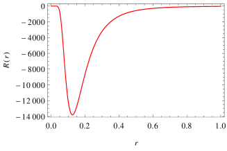
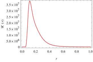
Figure 1: Graphical representation of functions $R(r)$ (left) and ${\cal K}(r)$ (right), in the nondegenerated case, for the values $\{m=80,q=10,c_{0}=1,c_{1}=2,\kappa^{2}=8\pi\}$ of the solution (38). The minimum value of the Ricci scalar is $R_{min}=-13,799.3$, and is located at $r=1/8$. The maximum of the Kretschmann scalar is ${\cal K}_{max}=3.78138\times 10^{7}$, and it happens at $r=0.11137$.

The Kretschmann scalar for the solution (38) is given by

$$\mathcal{K}(r)=R^{\alpha\beta\mu\nu}R_{\alpha\beta\mu\nu}=\frac{e^{-q^{2}/(mr)}}{4m^{2}r^{10}}\!\big{[}q^{8}-16mq^{6}r+96m^{2}q^{4}r^{2}-192m^{3}q^{2}r^{3}+192m^{4}r^{4}\big{]}.$$ (44)

We represent graphically the Kretschmann scalar in the right panel of Fig. 1. As we can see, the present solution is asymptotically flat and regular at space infinity. One has $\lim_{r\rightarrow\infty}\{e^{a}(r),\,e^{b}(r)\}=\{1,\,1\}$ and also $\lim_{r\rightarrow\infty}\{R(r),\,\mathcal{K}(r)\}=\{0,\,0\}$. The solution is clearly regular for finite nonzero values of $r$. Furthermore, the solution is also regular at the origin of the radial coordinate. One has $\lim_{r\rightarrow 0}\{e^{a}(r),\,e^{b}(r)\}=\{1,\,1\}$ and also $\lim_{r\rightarrow 0}\{R(r),\,\mathcal{K}(r)\}=\{0,\,0\}$. This shows explicitly the regularity of the solution.

Other interesting feature of the present solution is that it is a generalization of the solution presented in Eq. (17) of Ref. balart . This is seen by taking the particular case $c_{1}=0$, in which case our Eqs. (41) and (42) turn into the GR corresponding functions. Moreover, for $c_{1}=0$ and $c_{0}=\kappa^{2}/2$, the electric intensity (43) reduces to Eq. (19) of Ref. balart . Function $F^{10}(r)$ is plot in Fig. 2 (left panel), where it is seen the regularity of such a function at the central core. The asymptotic behavior for large $r$ of this and related functions is investigated in detail in Sec. A.1 of Appendix A.

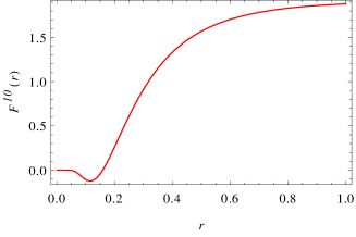
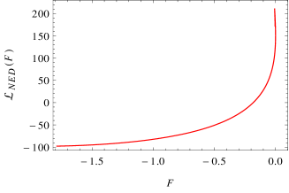
Figure 2: Graphical representation of functions $F^{10}(r)$ (left) and $\mathcal{L}_{NED}(F)$ (right), in the nondegenerated case, for the values $\{m=80,q=10,c_{0}=1,c_{1}=2,\kappa^{2}=8\pi\}$ of the solution (38).

A parametric plot of the Lagrangian density $\mathcal{L}_{NED}(F)$ in terms of the scalar $F$ is shown in the right panel of Fig. 2. The nonlinear character of such a relation becomes evident.

Functions $f(R)$ and its derivative $f_{R}(R)$, given respectively by Eqs. (41) and (42), are represented graphically in Fig. 3 for a particular choice of parameters. The nonlinear character of these curves reflects the fact that the gravity theory is not general relativity. It is clear they are well behaved functions at the central core. More details on these functions, in particular, on the asymptotic behavior at the spatial infinity are given in Appendix A.

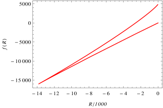
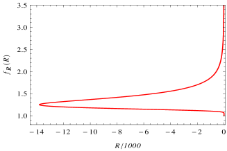
Figure 3: Graphical representation of functions $f(R)$ (left), and the function $f_{R}(R)$ (right), in the nondegenerated case, for the values $\{m=80,q=10,c_{0}=1,c_{1}=2,\kappa^{2}=8\pi\}$ of the solution (38). Both functions are defined, i.e., are real functions in the interval $R\in(0,-13,799.3]$.

In the regular black hole solution presented here, the metric functions $\{a(r),b(r)\}$, as well as the curvature scalars $\{R(r),\mathcal{K}(r)\}$, are identical to those presented in Ref. balart that considered GR coupled to NED. However, the new ingredient here, that guarantees we have a new solution, is exactly the function $f(R)$ given in Eq. (41). It enters the action integral modifying the gravitational part of the Lagrangian density, and generalizes also the nonlinear Lagrangian density $\mathcal{L}_{NED}(F)$, which is modified because of the generalized Faraday-Maxwell tensor (43).

A further interesting analysis is to check if the present solution satisfies the energy conditions for the $f(R)$ gravity santos . Substituting the function $M(r)$ of the present model from Eq. (37) into the energy conditions (25)-(29), and taking into account Eqs. (30)-(32), we find

$$NEC_{1}(r) = WEC_{1}(r)=0,$$ (45)

$$NEC_{2}(r) = WEC_{2}(r)=\frac{q^{2}e^{-q^{2}/(2mr)}}{4m\kappa^{2}r^{5}}\left(8mr-q^{2}\right),$$ (46)

$$SEC(r) = \frac{q^{2}e^{-q^{2}/(2mr)}}{2m\kappa^{2}r^{5}}\left(4mr-q^{2}\right),$$ (47)

$$DEC_{1}(r) = \frac{1}{2}DEC_{2}(r)=4\times DEC_{3}(r)=\frac{q^{2}}{\kappa^{2}r^{4}}e^{-q^{2}/(2mr)}\;.$$ (48)

Therefore, the energy conditions are all satisfied in the region $r\geq(q^{2}/4m)$, a lower bound on $r$ imposed by the strong energy condition, $SEC(r)\geq 0$. The weak energy condition is satisfied if $r\geq(q^{2}/8m)$, a lower bound on $r$ imposed by $WEC_{2}(r)\geq 0$. For the choices of parameters as those chosen for drawing the graphs of Figs. 1-3, namely $\{q=10,m=80\}$, it follows that the $SEC$ is violated for $r<0.3125$, while the $WEC$ is violated in the region $r<0.15625$. The region where these energy conditions are not satisfied is well inside the event horizon, since here we have $r_{H}=159.374$. It is well known that the $SEC$ is violated inside the horizon for the regular black hole solutions in GR theory, while the $WEC$ is in some cases violated throughout the spacetime. Restricting the preset solution (38) to the GR theory, i.e., taking $\{c_{0}=1,c_{1}=0\}$, we see that both the $SEC$ and the $WEC$ are not satisfied in the same regions as for the $f(R)$ gravity theory. This is easily explained by noticing that the energy conditions (25)-(29) do not depend on the parameters $c_{0}$ and $c_{1}$, and, moreover, the contributions from the functions $f(R)$ and $f_{R}$ to the effective energy density and pressures in Eqs. (30)-(32) are mutually canceled.

In the next section we shall present a new solution which violates only the $SEC$ in a limited region of the spacetime.

III.4 Second new regular black hole solution

Consider now the following ansatz for the mass function,

$$M(r)=m\left(1+\frac{q^{2}}{4\beta mr}\right)^{-2\beta},$$ (49)

where $m$, $q$, and $\beta$ are constant parameters. Such a model has been studied in Ref. balart in the context of GR coupled to NED theory. In GR it yields a black hole solution that is regular for $\beta\geq 3/2$ and that also satisfies the $WEC$ for $\beta\leq 3/2$. Hence, in the case where $\beta=3/2$ it results in a regular black hole which does satisfy the $WEC$. Since $\beta=3/2$ is a boundary value for regularity and to satisfy the $WEC$ within GR, we choose exactly this case to be analyzed within $f(R)$ gravity. Following the same steps as in the preceding section, we obtain

$$e^{a(r)}=e^{-b(r)}=1-\frac{432m^{4}r^{2}}{(q^{2}+6mr)^{3}},$$ (50)

$$\mathcal{K}(r)=\frac{4478976m^{8}}{\left(q^{2}+6mr\right)^{10}}\left(q^{8}+126m^{2}q^{4}r^{2}-216m^{3}q^{2}r^{3}+648m^{4}r^{4}\right)\,,$$ (51)

$$R(r)=-\frac{5184m^{4}q^{4}}{(q^{2}+6mr)^{5}},$$ (52)

$$F^{10}(r)=\frac{(6mr)^{3}}{\kappa^{2}\left(q^{2}+6mr\right)^{5}}\Bigg{\{}72c_{0}m^{2}q+\frac{c_{1}}{q}\left[18m^{2}r(5q^{2}+6mr)-\frac{(q^{2}+6mr)^{5}}{216m^{3}r^{2}}\right]\Bigg{\}}.$$ (53)

The present solution is asymptotically flat and regular at spatial infinity. One has $\displaystyle{\lim_{r\rightarrow\infty}\\ \{e^{a}(r),\,e^{b}(r)\}=\{1,\,1\}}$ and also $\displaystyle{\lim_{r\rightarrow\infty}\{R(r),\,\mathcal{K}(r)\}=\{0,\,0\}}$. The solution is also regular at the origin of the radial coordinate. One has $\displaystyle{\lim_{r\rightarrow 0}\{e^{a}(r),\,e^{b}(r)\}=\{1,\,1\}}$ and also $\displaystyle{\lim_{r\rightarrow 0}\{R(r),\,\mathcal{K}(r)\}=\{-5184m^{4}/q^{6},\,4478976m^{8}/q^{12}\}}$. This shows explicitly the regularity of the solution.

We may use Eq. (52) to get $r$ as a function of $R$ what, after being substituted into Eq. (15) and integrated, furnishes,

$$f(R) = c_{0}R+\frac{216m^{3}c_{1}}{q^{4}}-\frac{c_{1}}{12m}\left[2q^{2}R+5(162m^{4}q^{4})^{1/5}R^{4/5}\right].$$ (54)

The present solution for $f(R)$ shows clearly the deviation from GR due to the presence of the last term in Eq. (54). If we take $c_{1}=0$ and also $c_{0}=\kappa^{2}/2$ the GR theory is recovered. Notice also that in such a case the electric intensity (53) is identical to Eq. (49) of Ref. balart . The regularity of the functions at the central core is clear, while their behavior for large $r$ is investigated in detail in Sec. A.2 of Appendix A.

Here we analyse the energy conditions for the present solution. First we calculate the effective fluid quantities $\rho^{(eff)}$, $p_{r}^{(eff)}$ and $p_{t}^{(eff)}$ respectively from Eqs. (30)-(32). The result is

$$\rho^{(eff)}(r)=-p_{r}^{(eff)}(r)=\frac{1296\,q^{2}\,m^{4}}{\kappa^{2}\left(q^{2}+6m\,r\right)^{4}},$$ (55)

$$p_{t}^{(eff)}(r)=\frac{-q^{2}+6m\,r}{q^{2}+6m\,r\,}\rho^{(eff)}(r).$$ (56)

The behavior of each one of these functions in terms of the radial coordinate $r$ is shown in the left panel of Fig. 4. The radial pressure satisfies the relation $p_{r}^{(eff)}=-\rho^{(eff)}$, while the tangential pressure is positive for large $r$ and tends to $-\rho^{(eff)}$ at the center, where the effective fluid behaves approximately as an isotropic fluid satisfying a de Sitter equation of state, $p^{(eff)}\simeq-\rho^{(eff)}$.

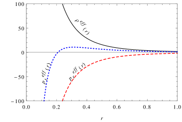
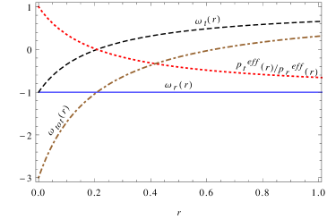
Figure 4: Graphical representation of the effective fluid quantities (left), and the functions $\omega_{r}=p_{r}^{(eff)}/\rho^{(eff)}$, $\omega_{t}=p_{t}^{(eff)}/\rho^{(eff)}$, $p_{t}^{(eff)}/p_{r}^{(eff)}$, and $\omega_{tot}=(p_{r}^{(eff)}+2p_{t}^{(eff)})/\rho^{(eff)}$ (right), in the nondegenerated case, for the values $\{m=80,q=10,c_{0}=1,c_{1}=2,\kappa^{2}=8\pi\}$ of the solution (49).

The right panel of Fig. 4 shows the ratios between the fluid quantities $\omega_{r}=p_{r}^{(eff)}/\rho^{(eff)}$ (solid line), $\omega_{t}=p_{t}^{(eff)}/\rho^{(eff)}$ (dashed line), and $p_{t}^{(eff)}/p_{r}^{(eff)}$ (dotted line). We plot also the ratio $\omega_{tot}=(p_{r}^{(eff)}+2p_{t}^{(eff)})/\rho^{(eff)}$ (dot-dashed line). It is seen that the ratio $\omega_{r}$ is constant, $\omega_{r}=-1$. The ratio $\omega_{t}$ varies from $-1$ (for $r=0$) to $1$ (for $r\rightarrow\infty)$. Similarly we get $-1\leq p_{t}^{(eff)}/p_{r}^{(eff)}\leq 1$, and $-3\leq\omega_{tot}\leq 1$.

Now, the energy conditions are found by substituting Eqs. (55)-(56) into Eqs. (25)-(29),

$$NEC_{1}(r) = WEC_{1}(r)=0,NEC_{2}(r)=WEC_{2}(r)=\frac{15552m^{5}q^{2}r}{\kappa^{2}(q^{2}+6mr)^{5}},$$ (57)

$$SEC(r) = \frac{2592m^{4}q^{2}(6mr-q^{2})}{\kappa^{2}(q^{2}+6mr)^{5}},$$ (58)

$$DEC_{1}(r) = \frac{1}{2}DEC_{2}(r)=\frac{1296m^{4}q^{2}}{\kappa^{2}(q^{2}+6mr)^{4}},$$

$$DEC_{3}(r) = \frac{2592m^{4}q^{4}}{\kappa^{2}(q^{2}+6mr)^{5}}\;.$$ (59)

The $NEC$, the $WEC$, and the $DEC$ are satisfied in the whole spacetime. On the other hand, the $SEC$ is not satisfied in the region $r<q^{2}/6m$. Once more, the $SEC$ is violated only in the central core, inside the event horizon. For the present case with $\{q=10,m=80\}$ it follows $q^{2}/6m=5/24\simeq 0.208333$, while the horizon is at $r_{H}=159.374$. In conclusion, the only violated energy condition is the $SEC$, reproducing essentially the same result as the corresponding solutions in GR coupled to NED theory. Again, we can see that the final expressions for the energy conditions do not depend on the parameters of the $f(R)$ gravity, i.e., they do not depend on $c_{0}$ and $c_{1}$ and, because of that, the results are the same in both theories.

IV Conclusion

We presented a class of solutions to the $f(R)$ gravity that generalizes some regular black hole solutions found in GR theory. The energy-momentum tensor comes from a nonlinear electrodynamics theory minimally coupled to the $f(R)$ gravity. We have shown explicitly two solutions that are regular throughout the spacetime. The metric of the two solutions approach the Reissner-Nordström metric far from the center, and possess also two free parameters corresponding to the ADM mass $m$ and to the electric charge $q$, respectively.

There is a third free parameter, $c_{1}$, related to the $f(R)$ function, such that the $f(R)$ theory reduces to general relativity when such a parameter vanishes. Moreover, by writing the resulting field equations for the $f(R)$ gravity in terms of the Einstein tensor, an effective energy-momentum tensor can be defined. The result is an anisotropic perfect fluid. The effective energy density, radial and tangent pressures for the two new solutions analyzed do not depend on the parameter $c_{1}$, suggesting that the properties of the matter-energy content of these solutions are similar to the corresponding geometries in general relativity theory.

In fact, the first solution violates the null and the weak energy conditions at the central region, well inside the event horizon, whose size is given by the radial coordinate characterized by the ratio $r_{0}=q^{2}/8m$. These conditions are violated in the region inside $r_{0}$, $r<q^{2}/8m$. It also violates the strong energy condition in a spherical region $r<q^{2}/4m$. The second of those solutions satisfies all but the strong energy condition that is violated in a central core well inside the event horizon, with $r<q^{2}/6m$. These results are in agreement with the singularity theorems of general relativity (see also zaslavskii ).

The regularity of the solutions is verified through the Ricci and Kretschmann scalars, assuring that there are no spacetime (curvature) singularities. The asymptotic behavior of the physical quantities at the spatial infinity is analyzed in view of the fact that two particular quantities, namely the derivative of the gravity Lagrangian density $df(R)/dR$ and the electric intensity $F^{10}$, diverge linearly at the limit $r\rightarrow\infty$. We show explicitly that all the relevant physical quantities for both of the solutions are bounded and well behaved in the asymptotic limit.

As a further development in this line of investigation, we expect that the method employed here may be used to obtain new interesting solutions, not only for regular black holes, generalizing those obtained in the context of general relativity. A more careful and detailed analysis related to the energy conditions in $f(R)$ seems necessary and, in fact, is one of the subjects under investigation by ourselves.

The present line of work also opens the possibility of new applications to local astrophysical phenomena such as the dark matter problem. For instance, a phenomenologically motivated mass function $M(r)$ may be proposed to fit the rotation curves of galaxies within some specific $f(R)$ model. Other application of the strategy followed in the present work is to simulate the mass distribution at the galactic bulge for a specific galaxy or some galaxy sample.

Acknowledgements: M. E. R. thanks Conselho Nacional de Desenvolvimento Científico e Tecnológico - CNPq, Brazil, Edital MCTI/CNPQ/Universal 14/2014 for partial financial support. V. T. Z. thanks Fundação de Amparo à Pesquisa do Estado de São Paulo (FAPESP), Grant No. 2011/18729-1, Conselho Nacional de Desenvolvimento Científico e Tecnológico of Brazil (CNPq), Grant No. 308346/2015-7, and Coordenação de Aperfeiçoamento do Pessoal de Nível Superior (CAPES), Brazil, Grant No. 88881.064999/2014-01.

Appendix A The asymptotic limit of the two new solutions

Here we explore the asymptotic limit $r\rightarrow+\infty$ of the two solutions presented above. The aim is to verify that the solutions are regular in such a limit. We have already commented in the text that all the physical quantities related to those solutions are regular everywhere in the spacetime. However, since some of the functions assume arbitrarily large values at $r\rightarrow\infty$ it is worth dwelling longer on this subject. To simplify analysis we define $r=1/x$ and then write all the functions in terms of the new variable $x$. The asymptotic limit of interest is now $x\rightarrow 0$.

A.1 Analysis of the first solution

Let us start with the metric function $e^{a(r)}$ of the first solution discussed in Sec. III.3. From Eq. (38),we get

$$e^{a(r)}=e^{a(1/x)}=1-2mx+q^{2}x^{2}+O\left(x^{3}\right).$$ (60)

After the hypothesis (13), $e^{b(r)}=e^{-a(r)}$, the last equation implies the metric functions of the present solution approach the Reissner-Nordström metric up to the second order in $1/r$.

On the other hand, function $df/dR$ given by Eq. (15) is clearly divergent at the radial infinity. However, what matters here is to verify whether such a divergence implies any kind of inconsistency in the physical and geometrical quantities regarding the solutions obtained in the present work. In fact, the Lagrangian density of the $f(R)$ gravity theory is the function $f(R)$ itself and, for the present case, it is given by Eq. (41). Expanding such a function in powers of $x=1/r$ one gets

$$f(R)=\frac{48m^{3}}{q^{4}}c_{1}-\frac{5q^{4}}{8m}c_{1}x^{4}+O\left(x^{5}\right).$$ (61)

Hence, the gravity Lagrangian density tends to a constant which means no diverge problems at the radial infinity.

Let us now analyse the functions related to the nonlinear electrodynamics theory employed here. The starting point is the Lagrangian $\mathcal{L}_{NED}$, whose asymptotic form, obtained from Eq. (19), for the model defined by Eq. (37), is

$$\mathcal{L}_{NED}=-\frac{24m^{3}}{q^{4}\kappa^{2}}c_{1}-\frac{c_{1}}{\kappa^{2}}x+O\left(x^{3}\right),$$ (62)

indicating that the NED Lagrangian density is also well behaved at the asymptotic limit. We see that the Lagrangian $\mathcal{L}_{NED}$ tends to a constant which exactly cancels the contribution from the gravity $f(R)$ Lagrangian density at first-order approximation, leading to a vanishing total Lagrangian density at the asymptotic limit, as usual for asymptotically flat spacetimes.

Now, taking the approximate form for the derivative of the NED Lagrangian density with respect to the field $F$, from (20), we get

$$\mathcal{L}_{F}=-\frac{q^{2}\kappa^{2}}{c_{1}}x^{3}+O\left(x^{4}\right),$$ (63)

which is also well defined at the asymptotic limit. The asymptotic form of the field $F^{10}(r)$ for the present solution is obtained from Eq. (43),

$$q\kappa^{2}F^{10}=3\,c_{1}m-\frac{c_{1}}{x}+\frac{q^{2}\left(16m\,c_{0}-5q^{2}c_{1}\right)x^{2}}{8m}+O(x^{3}).$$ (64)

Even though this function diverges with $r$, the electromagnetic energy density, defined by the right-hand side of Eq. (8) (divided by $\kappa^{2}$), $\rho_{EM}=\mathcal{L}_{NED}+\frac{q^{2}}{r^{4}}\mathcal{L}_{F}^{-1}$, is well behaved at $r\rightarrow\infty$. In fact, we have

$$\rho_{EM}=\frac{24m^{3}}{q^{4}}c_{1}+2c_{1}x-3mc_{1}x^{2}+O\left(x^{3}\right),$$ (65)

which approaches a constant at the asymptotic limit. Furthermore, the electric induction field $D^{\mu\nu}=\partial\mathcal{L}_{NED}/\partial F^{\mu\nu}=\mathcal{L}_{F}F^{\mu\nu}$ (see, e.g., burinskii ) is also well behaved at the spatial infinity. In fact, we obtain

$$D^{10}=\mathcal{L}_{F}\,F^{10}=qx^{2}-3\,m\,qx^{3}+O(x^{4}),$$ (66)

which vanishes according to $q/r^{2}$, as expected for a pointlike electric source in an asymptotically flat spacetime. As a matter of fact, this is a situation where the electric component of the Faraday-Maxwell tensor $F^{10}(r)$ does not fall-off as $1/r^{2}$ in an asymptotically Minkowskian spacetime (see, e.g., Ref. gonzalezetal for comparison with cases where the nonvanishing asymptotic behavior of $F^{10}(r)$ is connected to nonasymptotically flat spacetimes).

Moreover, we can verify that all the other physical quantities are also well behaved and regular everywhere in the spacetime. An important quantity is the effective energy density $\rho_{eff}$, given by Eq. (30). Its asymptotic limit is

$$\rho^{(eff)}=\frac{q^{2}}{\kappa^{2}}x^{4}+O\left(x^{5}\right),$$ (67)

what is well behaved at infinity and guarantees that the total energy of the solution is bounded. We have also performed the analysis of the effective pressures, $p_{r}^{(eff)}$ and $p_{t}^{(eff)}$, and verified that all the components of the effective energy-momentum tensor are well behaved functions at the asymptotic limit.

As a further consistency check, we investigate the behavior of the equations of motion at $r\rightarrow+\infty$ ($x\rightarrow 0$). After the choice (13) and, as a consequence, using the fact that $d^{2}f_{R}/dr^{2}=0$ (see Eq. (42)), it follows that Eq. (9) is identical to Eq. (8), so that only Eqs. (8) and (10) are independent relations. In such a limit, the left-hand-side of Eq. (8) is

$$\frac{24m^{3}}{q^{4}}c_{1}+2c_{1}x-3mc_{1}x^{2}+O\left(x^{3}\right),$$ (68)

showing no divergent term. The same result is found from the right-hand side of that equation. In turn, the asymptotic limit of the left-hand side of (10) is

$$\frac{24m^{3}}{q^{4}}c_{1}+c_{1}x+O\left(x^{3}\right),$$ (69)

which is the same as the right-hand side of that equation at the asymptotic limit. These results show that there are no divergent term in the equations of motion. Hence, even though the function $f_{R}(r)$ is unbounded at $r\rightarrow\infty$ all the equations of motion are well behaved everywhere.

At last we check the asymptotic form of the Ricci and Kretschmann scalars. From Eqs. (39) and (44) we get, respectively,

$$R=-\frac{q^{4}}{2m}x^{5}+O\left(x^{6}\right),$$ (70)

$$\mathcal{K}=48m^{2}x^{6}+O\left(x^{7}\right).$$ (71)

We finish this analysis emphasizing that all the geometric invariants and physical quantities of the solution presented in Sec. III.3 are regular, the equations of motions show no divergence and are well behaved everywhere in the spacetime. In this sense, we have found a fully consistent solution. The only unbounded functions are $f_{R}$ (see Eq. (42)) and the nonlinear electric intensity $F^{10}$, given by Eq. (43). The divergence of $f_{R}$ does not imply any kind of divergence on the physical and geometric properties of the spacetime. Moreover, the relevant physical quantities derived from the nonlinear electrodynamics are well behaved functions: the electromagnetic energy density is bounded, the energy-momentum tensor has no divergent terms, the total charge is finite (and constant), and the physical electric induction $D^{10}=\partial\mathcal{L}_{NED}/\partial F^{10}=\mathcal{L}_{F}\,F^{10}$ also behaves as expected for a pointlike electrostatic source.

A.2 Analysis of the second solution

Now we consider the asymptotic behavior of the solution derived from the ansatz of Eq. (49) [see also Eq. (50)] and presented in Sec. III.4. As above, we express the functions in terms of the new variable $x=1/r$.

As in the case of solution (38) the asymptotic form of the resulting metric at $r\rightarrow\infty$ is the Reissner-Nordström metric, with $g_{tt}=1/g_{rr}\simeq 1-2mx+q^{2}x^{2}-q^{4}x^{3}/3m$, where we fixed $\beta=3/2$.

The derivative of the gravitational Lagrangian density $f_{R}$ has the same form as in the case discussed in the last section, and so it diverges linearly with $r$. What we shall analyse once again is whether such a divergence introduces some inconsistency into the solution or not. First, using relation (16) and (49) we see that the Lagrangian density $f(R)$ is of the form

$$f(R)=\frac{216m^{3}}{q^{4}}c_{1}-\frac{5q^{4}}{6m}c_{1}x^{4}+O\left(x^{5}\right),$$ (72)

which tends to a constant.

The electromagnetic Lagrangian density $\mathcal{L}_{NED}$ also tends to a constant. In fact, using relations (19) and (49) we find

$$\mathcal{L}_{NED}=-\frac{108m^{3}}{q^{4}\kappa^{2}}c_{1}-\frac{c_{1}}{\kappa^{2}}x+O\left(x^{3}\right).$$ (73)

Once again, we see that, as $f(R)$, the Lagrangian $\mathcal{L}_{NED}$ is well behaved at the spatial infinity. As in the case of Sex. III.3, the total Lagrangian density $2\kappa^{2}\mathcal{L}_{NED}+f(R)$ vanishes at the asymptotic limit, a common behavior in asymptotically flat spaces.

Taking the same limit of the derivative of the electromagnetic Lagrangian density $\mathcal{L}_{F}$, from Eqs. (20) and (50) it results the same form as in Eq. (63), showing that it is a bounded function in the asymptotic limit.

The asymptotic form of the nonzero components of the Faraday-Maxwell tensor field $F^{10}(r)=-F^{01}(r)$ (the electric intensity) for the present solution is obtained from E. (53),

$$q\kappa^{2}F^{10}(r)=3\,c_{1}m-\frac{c_{1}}{x}+\frac{q^{2}\left(12m\,c_{0}-5q^{2}c_{1}\right)x^{2}}{6m}+O(x^{3}),$$ (74)

which has approximately the same form as in the first solution, and diverges linearly with $r$. However, the other electromagnetic quantities, the ones that have direct physical meaning, are well behaved function. For instance, the electromagnetic energy density (8) for the solution of section III.4, at the asymptotic region, assumes the form

$$\rho_{EM}=\frac{108m^{3}}{q^{4}}c_{1}+2c_{1}x-3mc_{1}x^{2}+O\left(x^{3}\right),$$ (75)

which tends to a constant. Moreover, the electric induction $D^{10}(r)$ is also well behaved at the spatial infinity. Indeed, we find the same leading terms as in Eq. (66), and the electric induction once again tends to $q/r^{2}$, as expected for a pointlike electric source in asymptotically flat spacetimes (see also the discussion following Eq. (64) above).

Other interesting physical quantity, the effective energy density, is well behaved too. Its asymptotic form is obtained from Eq. (30) [or from Eq. (55)] and the result is identical to the previous case, given by Eq. (67). A similar analysis of the effective pressures shows that all the components of the effective energy-momentum tensor are bounded function at the asymptotic limit. Another important consistency check is related to the equations of motion, since the divergence of functions $f_{R}$ and $F^{10}$ may induce singularities into the equations. Considering the solution (50) into Eq. (8), it follows that both sides of such an equation tend to

$$\frac{108m^{3}}{q^{4}}c_{1}+2c_{1}x-3mc_{1}x^{2}+O\left(x^{3}\right),$$ (76)

with no divergent terms and no other inconsistency is observed. As in the case of the first solution, Eq. (9) is identical to Eq. (8). In turn, the left-hand side of Eq. (10) gives

$$\frac{108m^{3}}{q^{4}}c_{1}+c_{1}x+O\left(x^{3}\right),$$ (77)

which is identical to the result obtained for the expression on the right-hand side of that equation. This shows there are no divergence nor inconsistencies in the equations of motions.

At last, the asymptotic form of the Kretschmann and Ricci scalars, from Eqs. (51) and (52), respectively, are

$$\mathcal{K}=48m^{2}x^{6}+O\left(x^{7}\right),$$ (78)

$$R=-\frac{2q^{4}}{3m}x^{5}+O\left(x^{6}\right).$$ (79)

With this we complete the analysis and verify that there no inconsistencies neither divergences of the physical and geometric properties of the spacetime.

References

- (1) R. Penrose, Gravitational collapse and space-time singularities, Phys. Rev. Lett. 14, 57 (1965); S. Hawking and R. Penrose, The singularities of gravitational collapse and cosmology, Proc. Roy. Soc. A 314, 529 (1970).
- (2) J.M. Bardeen, Non-singular general relativistic gravitational collapse, in Proceedings of the International Conference GR5, Tbilisi, U.S.S.R. (1968).
- (3) A. D. Sakharov, Initial stage of an expanding universe and appearance of a nonuniform distribution of matter, Sov. Phys. JETP 22, 241 (1966); E. Gliner, Algebraic properties of the energy-momentum tensor and vacuum-like states of matter, Sov. Phys. JETP 22, 378 (1966); Y. B. Zel’dovich, The cosmological constant and the theory of elementary particles, Sov. Phys. Usp. 11, 381 (1968).
- (4) E. Ayón-Beato and A. García, The Bardeen model as a nonlinear magnetic monopole, Phys. Lett. B 493, 149 (2000), [ gr-qc/0009077]; E. Ayón-Beato and A. García, Four-parametric regular black hole solution, Gen. Relativ. Gravit. 37, 635 (2005) [arXiv:hep-th/0403229]; E. Ayón-Beato and A. García, Regular black hole in general relativity coupled to nonlinear electrodynamics, Phys. Rev. Lett. 80, 5056 (1998), [gr-qc/9911046]; K. A. Bronnikov, Comment on regular black hole in general relativity coupled to nonlinear electrodynamics, Phys. Rev. Lett. 85, 4641 (2000); K. A. Bronnikov, Regular Magnetic Black Holes and Monopoles from Nonlinear Electrodynamics, Phys. Rev. D 63, 044005 (2001), [arXiv: gr-qc/0006014]; J. Matyjasek, Extremal limit of the regular charged black holes in nonlinear electrodynamics, Phys. Rev. D 70, 047504 (2004), [arXiv:gr-qc/0403109]; I. G. Dymnikova, Regular electrically charged vacuum structures with de Sitter centre in nonlinear electrodynamics coupled to general relativity, Classical Quantum Gravity 21, 4417 (2004), [arXiv:gr-qc/0407072].
- (5) S. Ansoldi, Spherical black holes with regular center: a review of existing models including a recent realization with Gaussian sources, arXiv:0802.0330 [gr-qc] (2008); [arXiv:0802.0330].
- (6) I. G. Dymnikova, Vacuum nonsingular black hole, Gen. Relativ. Gravit. 24, 235 (1992); I. G. Dymnikova, De Sitter-Schwarzschild black hole: its particlelike core and thermodynamical properties, Int. J. Mod. Phys. D 05, 529 (1996); I. G. Dymnikova, The algebraic structure of a cosmological term in spherically symmetric solutions, Phys. Lett. B 472, 33 (2000) [arXiv:gr-qc/9912116]; I. G. Dymnikova, A. Dobosz, M. L. Filchenkov, and A. Gromov, Universes inside a Lambda black hole, Phys. Lett. B 506, 351 (2001) [arXiv:gr-qc/0102032]; I. G. Dymnikova, Spherically symmetric space-time with regular de Sitter center, Int. J. Mod. Phys. D 12, 1015 (2003) [arXiv:gr-qc/0304110]; I. G. Dymnikova and E. Galaktionov, Stability of a vacuum non-singular black hole, Classical Quantum Gravity 22, 2331 (2005) [arXiv:gr-qc/0409049]; I. G. Dymnikova and M. Korpusika, Regular black hole remnants in de Sitter space, Phys. Lett. B 685, 12 (2010).
- (7) A. G. Riess it et al., Observational evidence from supernovae for an accelerating universe and a cosmological constant, Astron. J. 116, 1009 (1998),[arXiv:astro-ph/9805201]; S. Perlmutter et al., Discovery of a supernova explosion at half the age of the Universe and its cosmological implications, Nature (London) 391, 51 (1998),[arXiv:astro-ph/9712212]; S. Perlmutter et al., Measurements of Omega and Lambda from 42 high redshift supernovae, Astrophys. J. 517, 565 (1999), [arXiv:astro-ph/9812133].
- (8) J. A. Frieman, M. S. Turner, and D. Huterer, Dark energy and the accelerating Universe, Annu. Rev. Astron. Astrophys. 46, 385 (2008), [arXiv:0803.0982 ]; P. Astier and R. Pain, Observational evidence of the accelerated expansion of the Universe, Comptes Rendus Physique 13, 521 (2012), [arXiv:1204.5493].
- (9) M. P. Lima, S. Vitenti, and M. J. Rebouças, Energy conditions bounds and their confrontation with supernovae data, Phys. Rev. D 77, 083518 (2008), [arXiv:0802.0706]; J. Santos, J. S. Alcaniz, N. Pires, and M. J. Rebouças, Energy Conditions and Cosmic Acceleration, Phys. Rev. D 75, 083523 (2007), [arXiv:astro-ph/0702728]; J. Santos, J. S. Alcaniz, and M. J. Rebouças, Energy Conditions and Supernovae Observations, Phys. Rev. D 74, 067301 (2006), [arXiv:astro-ph/0608031]; J. Santos, J. S. Alcaniz, N. Pires, and M. J. Rebouças, Lookback time bounds from energy conditions, Phys. Rev. D 76, 043519 (2007), [arXiv:0706.1779]; J. Santos, J. S. Alcaniz, and M. J. Rebouças, Energy conditions constraints on a class of f(R)gravity, Int. J. Mod. Phys. D 19, 1315 (2010), [arXiv:0807.2443].
- (10) K. A. Bronnikov and J. C. Fabris, Regular phantom black holes, Phys. Rev. Lett. 96, 251101 (2006), [arXiv: gr-qc/0511109]; K. A. Bronnikov and I. Dymnikova, Regular homogeneous T-models with vacuum dark fluid, Classical Quantum Gravity 24, 5803 (2007), [arXiv:0705.2368]; M. Azreg-Aïnou, G. Clément, J. C. Fabris, and M. E. Rodrigues, Phantom black holes and sigma models, Phys. Rev. D 83 124001 (2011), [arXiv:1102.4093]; J. P. S. Lemos and V. T. Zanchin, Regular black holes: Electrically charged solutions, Reissner-Nordström outside a de Sitter core, Phys. Rev. D 83, 124005 (2011), [arXiv:1104.4790].
- (11) S. Nojiri and S. D. Odintsov, Introduction to modified gravity and gravitational alternative for dark energy, Int. J. Geom. Meth. Mod. Phys. 04 , 115 (2007), [arXiv:hep-th/0601213]; S. Nojiri and S. D. Odintsov, Introduction to modified gravity and gravitational alternative for dark energy, Int. J. Geom. Meth. Mod. Phys. 4,115 (2007), [arXiv:hep-th/0601213]; T. P. Sotiriou, V. Faraoni, f(R) Theories Of Gravity, Rev. Mod. Phys. 82, 451 (2010), [arXiv:0805.1726]; T. Clifton, P. G. Ferreira, A. Padilla, and C. Skordis, Modified gravity and cosmology, Phys. Rep. 513, 1 (2012), [arXiv:1106.2476].
- (12) A. De Felice, S. Tsujikawa, f(R) theories, Living Rev. Relativity 13, 3 (2010), [arXiv:1002.4928].
- (13) T. Harko, F. S. N. Lobo, S. Nojiri, and S. D. Odintsov, f(R,T) gravity, Phys. Rev. D 84, 024020 (2011), [arXiv:1104.2669]; M. Jamil, D. Momeni, M. Raza, and R. Myrzakulov, Reconstruction of some cosmological models in f(R,T) gravity, Eur. Phys. J. C 72 1999 (2012), [arXiv:1107.5807]; F. G. Alvarenga, A. de la Cruz-Dombriz, M. J. S. Houndjo, M. E. Rodrigues, and D. Sáez-Gómez, Dynamics of scalar perturbations in f(R,T) gravity, Phys. Rev. D 87, 103526 (2013), [arXiv:1302.1866].
- (14) K. Bamba, S. D. Odintsov, L. Sebastiani, and S. Zerbini, Finite-time future singularities in modified Gauss-Bonnet and F(R,G) gravity and singularity avoidance, Eur. Phys. J. C67 295 (2010), [arXiv:0911.4390]; S. Nojiri, S. D. Odintsov, A. Toporensky, and P. Tretyakov, Reconstruction and deceleration-acceleration transitions in modified gravity, Gen. Relativ Gravit. 42, 1997 (2010), [arXiv:0912.2488]; K. Bamba, C.-Q. Geng, S. Nojiri, and S. D. Odintsov, Equivalence of modified gravity equation to the Clausius relation, Europhys. Lett. 89, 50003 (2010), [arXiv:0909.4397]; M. J. S. Houndjo, M. E. Rodrigues, D. Momeni, and R. Myrzakulov, Exploring cylindrical solutions in modified f(G) gravity, Can. J. Phys. 92, 1528 (2014), [arXiv:1301.4642]; M. E. Rodrigues, M. J. S. Houndjo, D. Momeni, and R. Myrzakulov, A type of Levi-Civita’s solution in modified Gauss-Bonnet gravity, Can. J. Phys. 92, 173 (2014), [arXiv:1212.4488].
- (15) S. Nojiri and S. D. Odintsov, Modified gravity with negative and positive powers of the curvature: unification of the inflation and of the cosmic acceleration, Phys. Rev. D 68, 123512 (2003), [hep-th/0307288]; S. Nojiri and S. D. Odintsov, Modified Gauss-Bonnet theory as gravitational alternative for dark energy, Phys. Lett. B 631, 1 (2005), [hep-th/0508049]; G. Cognola, E. Elizalde, S. Nojiri, S. D. Odintsov, and S. Zerbini, Dark energy in modified Gauss-Bonnet gravity: late-time acceleration and the hierarchy problem, Phys. Rev. D 73, 084007 (2006), [hep-th/0601008]; A. De Felice and T. Suyama, Vacuum structure for scalar cosmological perturbations in Modified Gravity Models, J. Cosmol. Astropart. Phys. 06 (2009) 034, [arXiv:0904.2092]; A. De Felice and S. Tsujikawa, Construction of cosmologically viable f(G) gravity models, Phys. Lett. B 675, 1 (2009), [arXiv:0810.5712]; E. Elizalde, R. Myrzakulov, V. V. Obukhov, and D. Sáez-Gómez, LambdaCDM epoch reconstruction from F(R,G) and modified Gauss-Bonnet gravities, Classical Quantum Gravity 27, 095007 (2010), [arXiv:1001.3636].
- (16) S. D. Odintsov and D. Sáez-Gómez, gravity phenomenology and CDM universe, Phys. Lett. B 725, 437 (2013), [arXiv:1304.5411].
- (17) K. Bamba, S. Nojiri, and S. D. Odintsov, The Universe future in modified gravity theories: Approaching the finite-time future singularity, J. Cosmol. Astropart. Phys. 10 (2008) 045, [arXiv:0807.2575]; K. Bamba, S. D. Odintsov, L. Sebastiani, and S. Zerbini, Finite-time future singularities in modified Gauss-Bonnet and F(R,G) gravity and singularity avoidance, Eur. Phys. J. C 67, 295 (2010), [arXiv:0911.4390]; K. Bamba and S. D. Odintsov, Inflation and late-time cosmic acceleration in non-minimal Maxwell-F(R) gravity and the generation of large-scale magnetic fields, J. Cosmol. Astropart. Phys. 04 (2008) 024, [arXiv:0801.0954].
- (18) F. W. Hehl, J. D. McCrea, E. W. Mielke, and Y. Ne’eman, Metric affine gauge theory of gravity: Field equations, Noether identities, world spinors, and breaking of dilation invariance, Phys. Rep. 258, 1 (1995), [arXiv:gr-qc/9402012]; R. Aldrovandi and J. G. Pereira, An Introduction to Teleparallel Gravity (Instituto de Física Teórica, São Paulo, 2010), [www.ift.unesp.br/users/jpereira/tele.pdf]; R. Aldrovandi, J. G. Pereira, and K. H. Vu, Selected Topics in Teleparallel Gravity, Braz. J. Phys. 34 (2004), [arXiv:gr-qc/0312008]; J. W. Maluf, The teleparallel equivalent of general relativity, Ann. Phys. (Berlin) 525, 339 (2013), [arXiv:1303.3897].
- (19) R. Ferraro and F. Fiorini, Modified teleparallel gravity: Inflation without inflaton, Phys. Rev. D 75, 084031 (2007), [arXiv:gr-qc/0610067]; J. B. Dent, S. Dutta, and E. N. Saridakis, f(T) gravity mimicking dynamical dark energy. Background and perturbation analysis , J. Cosmol. Astropart. Phys. 01 (2011) 009, [arXiv:1010.2215]; B. Li, T. P. Sotiriou, and J. D. Barrow, f(T) gravity and local Lorentz invariance, Phys. Rev. D 83, 064035 (2011), [arXiv:1010.1041]; M.E. Rodrigues, M.J.S. Houndjo, D. Sáez-Gómez, and F. Rahaman, Anisotropic Universe Models in f(T) Gravity, Phys. Rev. D 86, 104059 (2012), [arXiv:1209.4859 [gr-qc]]; C. Xu, E. N. Saridakis, and G. Leon, Phase-Space analysis of Teleparallel Dark Energy, J. Cosmol. Astropart. Phys. 07 (2012) 005, [arXiv:1202.3781]; C. G. Boehmer, T. Harko, and F. S.N. Lobo, ıt Wormhole geometries in modified teleparallel gravity and the energy conditions , Phys. Rev. D 85, 044033 (2012), [arXiv:1110.5756]; S. Basilakos, S. Capozziello, M. De Laurentis, A. Paliathanasis, and M. Tsamparlis, Noether symmetries and analytical solutions in f(T)-cosmology: A complete study , Phys. Rev. D 88, 103526 (2013), [arXiv:1311.2173]; K. Bamba, S. D. Odintsov, and D. Sáez-Gómez, Conformal symmetry and accelerating cosmology in teleparallel gravity, Phys. Rev. D 88, 084042 (2013), [arXiv:1308.5789]; T. Harko, F. S. N. Lobo, G. Otalora, and E. N. Saridakis, Nonminimal torsion-matter coupling extension of f(T) gravity , Phys. Rev. D 89, 124036 (2014), [arXiv:1404.6212]; J. Aftergood and A. DeBenedictis, Matter conditions for regular black holes in f(T) gravity, Phys. Rev. D 90, 124006 (2014), [arXiv:1312.1739].
- (20) F. Kiani and K. Nozari, Energy conditions in F(T,) gravity and compatibility with a stable de Sitter solution, Phys. Lett. B 728, 554 (2014), [arXiv:1309.1948]; T. Harko, F. S. N. Lobo, G. Otalora, and E. N. Saridakis, gravity and cosmology, J. Cosmol. Astropart. Phys. 12 (2014) 021, [arXiv:1405.0519].
- (21) G. Kofinas and E. N. Saridakis, Teleparallel equivalent of Gauss-Bonnet gravity and its modifications, Phys. Rev. D 90, 084044 (2014), [arXiv:1404.2249].
- (22) E. L. B. Junior and M. E. Rodrigues, Generalized teleparallel theory, Eur. Phys. J. C 76, 376 (2016), [arXiv:1509.03267 [gr-qc]].
- (23) K. Bamba, S. Capozziello, S. Nojiri, and S. D. Odintsov, Dark energy cosmology: the equivalent description via different theoretical models and cosmography tests, Astrophys. Space Sci. 342, 155 (2012), [arXiv:1205.3421].
- (24) R. Zheng and Q. G. Huang, Growth factor in f(T) gravity, J. Cosmol. Astropart. Phys. 03 (2011) 002, [arXiv:1010.3512]; N. Paul, S. N. Chakrabarty, and K. Bhattacharya, Cosmological bounces in spatially flat FRW spacetimes in metric f(R) gravity, J. Cosmol. Astropart. Phys. 10 (2014) 009, [arXiv:1405.0139].
- (25) M. Born and L. Infeld, Foundations of the New Field Theory, Proc. R. Soc. A 144, 425 (1934).
- (26) A. Peres, Nonlinear Electrodynamics in General Relativity, Phys. Rev. 122, 273 (1961).
- (27) G. W. Gibbons and D. A. Rasheed, Sl(2,R) invariance of nonlinear electrodynamics coupled to an axion and a dilaton, Phys. Lett. B 365, 46 (1996), [hep-th/9509141]; E. Ayón-Beato and A. García, New regular black hole solution from nonlinear electrodynamics, Phys.Lett. B 464, 25 (1999), [hep-th/9911174]; E. Ayón-Beato and A. García, Regular black hole in general relativity coupled to nonlinear electrodynamics, Phys. Rev. Lett. 80, 5056 (1998), [arXiv:gr-qc/9911046]; K. A. Bronnikov, Regular magnetic black holes and monopoles from nonlinear electrodynamics, Phys. Rev. D 63, 044005 (2001), [arXiv:gr-qc/0006014]; I. Dymnikova, Regular electrically charged structures in nonlinear electrodynamics coupled to general relativity, Classical Quantum Gravity 21, 4417 (2004), [arXiv:gr-qc/0407072]; F. S. N. Lobo, and A. V. B. Arellano, Gravastars supported by nonlinear electrodynamics, Classical Quantum Gravity 24, 1069 (2007), [gr-qc/0611083]; L. Balart, Energy distribution of 2+1 dimensional black holes with nonlinear electrodynamics, Mod. Phys. Lett. A 24, 2777 (2009), [arXiv:0904.4318]; A. García, E. Hackmann, C. Lammerzahl, and A. Macias, No-hair conjecture for Einstein-Plebanski nonlinear electrodynamics static black holes, Phys. Rev. D 86, 024037 (2012); G. J. Olmo and D. Rubiera-Garcia, Palatini f(R) Black Holes in Nonlinear Electrodynamics, Phys. Rev. D 84, 124059 (2011), [arXiv:1110.0850]; L. Balart and E. C. Vagenas, Regular black holes with a nonlinear electrodynamics source, Phys. Rev. D 90, 124045 (2014), [arXiv:1408.0306]; J. A. R. Cembranos, A. de la Cruz-Dombriz, and J. Jarillo, Reissner-Nordström black holes in the inverse electrodynamics model, J. Cosmol. Astropart. Phys. 02 (2015) 042, [arXiv:1407.4383].
- (28) D. Psaltis, D. Perrodin, R. Dienes, and I. Mocioiu, Kerr black holes are not unique to general relativity, Phys. Rev. Lett. 100, 091101 (2008); Phys. Rev. Lett. 100, 119902(E) (2008), [arXiv:0710.4564]; A. de la Cruz-Dombriz, A. Dobado, and A. L. Maroto, Black holes in theories, Phys. Rev D 80, 124011 (2009), [arXiv:0907.3872]; A. Aghmohammadi, K. Saaidi, M. R. Abolhassani, and A. Vajdi, Spherical symmetric solution in model around charged black hole, Int. J. Theor. Phys. 49, 709 (2010), [arXiv:1001.4148]; S. H. Mazharimousavi and M. Halilsoy, Black hole solutions in f(R) gravity coupled with non-linear Yang-Mills field, Phys. Rev. D 84, 064032 (2011), [arXiv:1105.3659]; S. H. Mazharimousavi, M. Halilsoy, and T. Tahamtan, Solutions for f(R) gravity coupled with electromagnetic field, Eur. Phys. J. C 72, 1851 (2012), [arXiv:1110.5085]; J. A. R. Cembranos, A. de la Cruz-Dombriz, and P. Jimeno-Romero, Kerr-Newman black holes in f(R) theories, Int. J. Geom. Meth. Mod. Phys. 11, 1450001 (2014), [arXiv:1109.4519].
- (29) G. J. Olmo and D. Rubiera-Garcia, Black holes with electric charge in Palatini theories of gravity, AIP Conf. Proc. 1458, 511 (2012); G. J. Olmo and D. Rubiera-Garcia, Nonsingular black holes in quadratic Palatini gravity, Eur. Phys. J. C 72, 2098 (2012), [arXiv:1112.0475]; G. J. Olmo and D. Rubiera-Garcia, Reissner-Nordström black holes in extended Palatini theories, Phys. Rev. D 86, 044014 (2012), [arXiv:1207.6004]; G. J. Olmo and D. Rubiera-Garcia, Nonsingular black holes in theories, Universe 2015, 1(2), 173 (2015), [arXiv:1509.02430]; C. Bambi, A. Cardenas-Avendano, G. J. Olmo and D. Rubiera-Garcia, Wormholes and nonsingular space-times in Palatini gravity, Phys. Rev. D 93, 064016 (2016), [arXiv:1511.03755 [gr-qc]].
- (30) J. Wainwright and P. E. A. Yaremovicz, Killing vector fields and the Einstein-Maxwell field equations with perfect fluid source, Gen. Relativ. Gravit. 7, 345 (1976) ; J. Wainwright and P. E. A. Yaremovicz, Symmetries and the Einstein-Maxwell field equations. The null field case, Gen. Relativ. Gravit. 7, 595 (1976).
- (31) M. Visser, Lorentzian wormholes: from Einstein to Hawking, (Springer, New York, 1996).
- (32) J. Santos, J. S. Alcaniz, M. J. Rebouças, and F. C. Carvalho, Energy conditions in f(R)-gravity, Phys. Rev. D 76, 083513 (2007), [arXiv:0708.0411]; F. D. Albareti, J. A. R. Cembranos, A. de la Cruz-Dombriz, and A. Dobado, On the non-attractive character of gravity in f(R) theories, J. Cosmol. Astropart. Phys. 07 (2013) 009, [arXiv:1212.4781 [gr-qc]]; F. D. Albareti, J. A. R. Cembranos, A. de la Cruz-Dombriz, and A. Dobado, The Raychaudhuri equation in homogeneous cosmologies, J. Cosmol. Astropart. Phys. 03 (2014) 012, [arXiv:1401.7926 [gr-qc]]; S. Capozziello, F. S. N. Lobo, and J. P. Mimoso, Generalized energy conditions in extended theories of gravity, Phys. Rev. D 91, 124019 (2015), [arXiv:1407.7293 [gr-qc]].
- (33) H. Culetu, On a regular modified Schwarzschild spacetime, [arXiv:1305.5964 [gr-qc]]; H. Culetu, On a regular charged black hole with a nonlinear electric source, Int. J. Theor. Phys.54, 2855 (2015), [arXiv:1408.3334 [gr-qc]].
- (34) L. Balart and E. C. Vagenas, Regular black holes with a nonlinear electrodynamics source, Phys. Rev. D 90, 124045 (2014), [arXiv:1408.0306 [gr-qc]].
- (35) T. P. Dence, A Brief Look into the Lambert W Function, Applied Mathematics 4, 887 (2013).
- (36) O. B. Zaslavskii, Regular black holes and energy conditions, Phys. Lett. B 688, 278 (2010), [arXiv:1004.2362 [gr-qc]].
- (37) A. Burinskii and Sergi R. Hildebrandt, New type of regular black holes and particlelike solutions from nonlinear electrodynamics, Phys. Rev. D 65, 104017 (2002), [hep-th/0202066].
- (38) H. A. González, M. Hassan̈e†m, and C. Martínez, Thermodynamics of charged black holes with a nonlinear electrodynamics source, Phys. Rev. D 80, 104008 (2009), [arXiv:0909.1365].
- (39) G. Cognola, E. Elizalde, L. Sebastiani and S. Zerbini, Topological electro-vacuum solutions in extended gravity, Phys. Rev. D 86, 104046 (2012), [arXiv:1208.2540 [gr-qc]].
- (40) L. Sebastiani and S. Zerbini, Static Spherically Symmetric Solutions in F(R) Gravity, Eur. Phys. J. C 71, 1591 (2011) , [arXiv:1012.5230 [gr-qc]].