Frustrated Heisenberg antiferromagnet on the honeycomb lattice with spin quantum number $s\geq 1$

Abstract

The ground-state (GS) phase diagram of the frustrated spin-$s$ $J_{1}$–$J_{2}$–$J_{3}$ Heisenberg antiferromagnet on the honeycomb lattice is studied using the coupled cluster method implemented to high orders of approximation, for spin quantum numbers $s=1,\,\frac{3}{2},\,2\,,\frac{5}{2}$. The model has antiferromagnetic (AFM) nearest-neighbour, next-nearest-neighbour and next-next-nearest-neighbour exchange couplings (with strength $J_{1}>0$, $J_{2}>0$ and $J_{3}>0$, respectively). We specifically study the case $J_{3}=J_{2}=\kappa J_{1}$, in the range $0\leq\kappa\leq 1$ of the frustration parameter, which includes the point of maximum classical ($s\rightarrow\infty$) frustration, viz., the classical critical point at $\kappa_{{\rm cl}}=\frac{1}{2}$, which separates the Néel phase for $\kappa<\kappa_{{\rm cl}}$ and the collinear striped AFM phase for $\kappa>\kappa_{{\rm cl}}$. Results are presented for the GS energy, magnetic order parameter and plaquette valence-bond crystal (PVBC) susceptibility. For all spins $s\geq\frac{3}{2}$ we find a quantum phase diagram very similar to the classical one, with a direct first-order transition between the two collinear AFM states at a value $\kappa_{c}(s)$ which is slightly greater than $\kappa_{{\rm cl}}$ [e.g., $\kappa_{c}(\frac{3}{2})\approx 0.53(1)$] and which approaches it monotonically as $s\rightarrow\infty$. By contrast, for the case $s=1$ the transition is split into two such that the stable GS phases are one with Néel AFM order for $\kappa<\kappa_{c_{1}}=0.485(5)$ and one with striped AFM order for $\kappa>\kappa_{c_{2}}=0.528(5)$, just as in the case $s=\frac{1}{2}$ (for which $\kappa_{c_{1}}\approx 0.47$ and $\kappa_{c_{2}}\approx 0.60$). For both the $s=\frac{1}{2}$ and $s=1$ models the transition at $\kappa_{c_{2}}$ appears to be of first-order type, while that at $\kappa_{c_{1}}$ appears to be continuous. However, whereas in the $s=\frac{1}{2}$ case the intermediate phase appears to have PVBC order over the entire range $\kappa_{c_{1}}<\kappa<\kappa_{c_{2}}$, in the $s=1$ case PVBC ordering either exists only over a very small part of the region or, more likely, is absent everywhere.

1 Introduction

Quantum spin-lattice models, in which the sites of a give regular periodic lattice are all occupied by magnetic ions with spin quantum number $s$, offer a rich arena for the study of exotic ground-state (GS) phases that are not present in their classical ($s\rightarrow\infty$) counterparts. Whereas interactions between the classical spins give rise to magnetic ground states in which the spins are ordered such that each individual spin is oriented in a specific direction, quantum fluctuations can act either to diminish the corresponding magnetic order parameter (viz., the average local onsite magnetization) or to destroy it altogether. In the former case, where the long-range order (LRO) is only partially reduced, such quasiclassical magnetically ordered states spontaneously break both the SU(2) spin-rotation and time-reversal symmetries.

By contrast, such intrinsically quantum-mechanical states as the various valence-bond crystalline (VBC) phases, in which specific combinations of the lattice spins combine into spin singlets, have zero magnetic order and break neither of the SU(2) spin-rotation and time-reversal symmetries, although they still break some lattice symmetries. Yet other states exist in which, for example, time-reversal symmetry is preserved, so that magnetic order is definitely absent, but for which the SU(2) spin-rotation symmetry is still broken. These are the so-called multipolar or spin-nematic phases. Finally, of course, one also has the possibility of quantum spin-liquid (QSL) phases that preserve all of the symmetries, including the lattice symmetries.

For a given regular lattice in $d$ spatial dimensions, one is usually interested in the interplay between frustration (which may be tuned, for example, by varying the relative strengths of competing interactions in the model Hamiltonian that separately tend to promote different forms of magnetic LRO) and quantum fluctuations. In broad terms quantum fluctuations are larger for lower values of both the spatial dimensionality $d$ and the spin quantum number $s$. They are typically also larger, for given spatial dimensionality $d$, for lattices with smaller values of the coordination number $z$.

For the case of $d=1$ isotropic Heisenberg chain systems the Mermin-Wagner theorem [1] excludes the possibility of GS magnetic order even at zero temperature ($T=0$), since it is impossible to break a continuous symmetry for any such system. The Mermin-Wagner theorem similarly implies the absence of magnetic LRO in any $d=2$ isotropic Heisenberg system at all nonzero temperatures ($T>0$). The behaviour and GS quantum phase structure of two-dimensional (2D) spin-lattice models at $T=0$ has thus come to occupy a special role in the study of quantum phase transitions.

Spin-lattice systems are said to be frustrated when constraints are present that preclude the formation of a GS phase which satisfies all of the (generally, pairwise) interactions among the spins. Frustration is strongly associated with macroscopic degeneracy of the GS phase, with the consequent existence of strong quantum fluctuations among the states in the degenerate manifold. Either quantum or thermal fluctuations can then, in such a situation, suppress magnetic LRO, and the possibility of such exotic non-classical states as those discussed above forming the stable GS phase under certain conditions is heightened. The low coordination number, $z=3$, of the honeycomb lattice further enhances the quantum fluctuations, and thereby makes it a special 2D spin-lattice model candidate for the study of its $T=0$ GS quantum phase diagram when dynamical frustration is introduced via competing interactions.

In the present paper we study the so-called $J_{1}$–$J_{2}$–$J_{3}$ model on the honeycomb lattice with antiferromagnetic (AFM) Heisenberg exchange interactions between pairs of nearest-neighbour (NN) spins (of strength $J_{1}$), next-nearest-neighbour (NNN) spins (of strength $J_{2}$), and next-next-nearest-neighbour (NNNN) spins (of strength $J_{3}$). Even in the classical ($s\rightarrow\infty$) limit the model has a rich phase diagram [2, 3], as we discuss further in Sec. 2 below. In the case where all three bonds are AFM in nature (i.e., $J_{i}>0$; $i=1,2,3$), the classical system exhibits two collinear AFM phases, namely the so-called Néel and striped phases, as well as a spiral phase. The three phases meet in a triple point at $J_{3}=J_{2}=J_{1}/2$ (see, e.g., Refs. [3, 4]). This is the point of maximum classical frustration, where the classical GS phase has macroscopic degeneracy. For the present study we consider the model along the line $J_{3}=J_{2}\equiv\kappa J_{1}$ for the case $J_{1}>0$, as a function of the frustration parameter $\kappa$ in the range $0\leq\kappa\leq 1$. The classical ($s\rightarrow\infty$) version of the model thus has a single quantum phase transition in its $T=0$ phase diagram at $\kappa_{{\rm cl}}=\frac{1}{2}$. For $\kappa<\kappa_{{\rm cl}}$ the stable GS phase is the Néel AFM phase, whereas for $\kappa>\kappa_{{\rm cl}}$ the stable GS phase is the striped AFM phase. In fact, at $T=0$, there actually exists an infinite family of non-coplanar states, all of which are degenerate in energy with the striped state. However, it is asserted [3] that both thermal and quantum fluctuations break this degeneracy in favour of the collinear striped state, at least in the large-$s$ limit [2].

Whereas the spin-$\frac{1}{2}$ $J_{1}$–$J_{2}$–$J_{3}$ model on the honeycomb lattice, or particular cases of it (e.g., when $J_{3}=J_{2}$ or $J_{3}=0$), have been investigated by many authors with a variety of theoretical tools (see, e.g., Refs. [2, 3, 5, 6, 4, 7, 8, 9, 10, 11, 12, 13, 14, 15, 16, 17, 18, 19, 20, 21, 22, 23, 24]), there are far fewer studies of the model in the case $s>\frac{1}{2}$. A particular exception is a very recent study [25] of the $s=1$ $J_{1}$–$J_{2}$ model (i.e., when $J_{3}=0$) on the honeycomb lattice, using the density-matrix renormalization group (DMRG) method. Our specific aim here is to extend earlier work using the coupled cluster method (CCM) applied to the spin-$\frac{1}{2}$ version of the $J_{1}$–$J_{2}$–$J_{3}$ model on the honeycomb lattice along the line $J_{3}=J_{2}$ [9, 15, 17], to cases $s>\frac{1}{2}$. In particular, we now compare results for the case $s=\frac{1}{2}$ with those for $s=1,\,\frac{3}{2},\,2,\,\frac{5}{2}$.

We note that by now there exist many experimental realizations of frustrated honeycomb-lattice systems with AFM interactions. These include such magnetic compounds as Na₃Cu₂SbO₆ [26], InCu_2/3V_1/3O₃ [27], $\beta$-Cu₂V₂O₇ [28], and Cu₅SbO₆ [29], in each of which the $s=\frac{1}{2}$ Cu²⁺ ions are situated on the sites of weakly coupled honeycomb-lattice layers. The iridates A₂IrO₃ (A $=$ Na, Li) [30, 31, 32, 33] are also believed to be magnetically ordered Mott insulators in which the Ir⁴⁺ ions form effective $s=\frac{1}{2}$ moments arrayed on weakly-coupled honeycomb-lattice layers. Other similar honeycomb materials include, for example, the families of compounds BaM₂(XO₄)₂ (M $=$ Co, Ni; X $=$ P, As) [34] and Cu₃M₂SbO₆ (M $=$ Co, Ni) [35]. In both of these families the magnetic ions M²⁺ are again disposed in weakly-coupled layers where they occupy the sites of a honeycomb lattice. In both families the Ni²⁺ ions appear to take the high-spin value $s=1$, whereas the Co²⁺ ions appear to take the low-spin value $s=\frac{1}{2}$ in the former family BaCo₂(XO₄)₂ and the high-spin value $s=\frac{3}{2}$ in the latter compound Cu₃Co₂SbO₆. As a last example of an $s=\frac{3}{2}$ honeycomb-lattice AFM material, we also mention the layered compound Bi₃Mn₄O₁₂(NO₃) [36, 37] in which the spin-$\frac{3}{2}$ Mn⁴⁺ ions sit on the sites of the honeycomb layers.

The remainder of the paper is organized as follows. In Sec. 2 we discuss further the model itself, before we give a brief description in Sec. 3 of the CCM formalism that we apply to it. The results are then presented in Sec. 4, and we conclude in Sec. 5 with a discussion and summary.

2 The model

The Hamiltonian of the $J_{1}$–$J_{2}$–$J_{3}$ model on the honeycomb lattice is given by

$$H=J_{1}\sum_{\langle i,j\rangle}\mathbf{s}_{i}\cdot\mathbf{s}_{j}+J_{2}\sum_{\langle\langle i,k\rangle\rangle}\mathbf{s}_{i}\cdot\mathbf{s}_{k}+J_{3}\sum_{\langle\langle\langle i,l\rangle\rangle\rangle}\mathbf{s}_{i}\cdot\mathbf{s}_{l}\,,$$ (1)

where the sums over $\langle i,j\rangle$, $\langle\langle i,k\rangle\rangle$ and $\langle\langle\langle i,l\rangle\rangle\rangle$ run over all NN, NNN and NNNN bonds, respectively, on the lattice, counting each pair of spins once and once only in each of the three sums. Each site $i$ of the honeycomb lattice carries a spin-$s$ particle described by the SU(2) spin operator ${\bf s}_{i}\equiv(s^{x}_{i},s^{y}_{i},s^{z}_{i})$, with ${\bf s}^{2}_{i}=s(s+1)$, and, for the cases considered here, $s=1,\,\frac{3}{2},\,2,\frac{5}{2}$. The lattice and the Heisenberg exchange bonds are illustrated in Fig. 1(a).

   

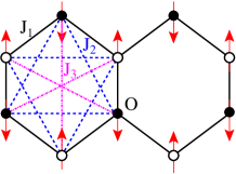
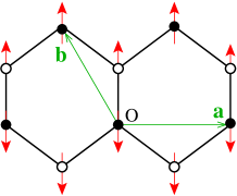
Figure 1: The $J_{1}$–$J_{2}$–$J_{3}$ model on the honeycomb lattice, showing (a) the bonds ($J_{1}=$ —–, $J_{2}=$ - - -, $J_{3}=$ - $\cdot$ - ) and the Néel state, and (b) the triangular Bravais lattice vectors $\mathbf{a}$ and $\mathbf{b}$ and one of three equivalent striped states. Sites on the two triangular sublattices ${\cal A}$ and ${\cal B}$ are shown by filled and empty circles respectively, and the spins are represented by the (red) arrows on the lattice sites.

For the present study we are interested in the case where each of the three types of bonds is AFM in nature (i.e., $J_{m}>0$; $m=1,2,3$). Without loss of generality we may put $J_{1}\equiv 1$ to set the overall energy scale, and we will specifically consider the case where $J_{3}=J_{2}\equiv\kappa J_{1}$, in the interesting window $0\leq\kappa\leq 1$ of the frustration parameter $\kappa$.

The honeycomb lattice is bipartite, but comprises two triangular Bravais sublattices ${\cal A}$ and ${\cal B}$. The basis vectors $\mathbf{a}=\sqrt{3}d\hat{x}$ and $\mathbf{b}=(-\sqrt{3}\hat{x}+3\hat{z})d/2$ are illustrated in Fig. 1(b), where the lattice is defined to lie in the $xz$ plane as shown, and where $d$ is the lattice spacing (i.e., the distance between NN sites). The unit cell $i$ at position vector $\mathbf{R}_{i}=m_{i}\mathbf{a}+n_{i}\mathbf{b}$, where $m_{i},\,n_{i}\in\mathbb{Z}$, now comprises the two sites at $\mathbf{R}_{i}\in{\cal A}$ and $(\mathbf{R}_{i}+d\hat{z})\in{\cal B}$. The reciprocal lattice vectors corresponding to the real-space vectors $\mathbf{a}$ and $\mathbf{b}$ are thus $\boldsymbol{\alpha}=2\pi(\sqrt{3}\hat{x}+\hat{z})/(3d)$ and $\boldsymbol{\beta}=4\pi/(3d)\hat{z}$. The Wigner-Seitz unit cell and the first Brillouin zone are thus the parallelograms formed, respectively, by the pairs of vectors $(\mathbf{a}$, $\mathbf{b})$ and $(\boldsymbol{\alpha}$, $\boldsymbol{\beta})$. Both may equivalently be taken as being centred on a point of sixfold rotational symmetry in their respective spaces. Thus, the Wigner-Seitz unit cell may be taken as being bounded by the sides of a primitive hexagon of side length $d$ as in Fig. 1. In this case the first Brillouin zone is also a hexagon, now of side length $4\pi/(3\sqrt{3}d)$, and which is also rotated by 90^∘ with respect to the Wigner-Seitz hexagon.

The classical ($s\rightarrow\infty$) version of the $J_{1}$–$J_{2}$–$J_{3}$ model of Eq. (1) on the honeycomb lattice already itself displays a rich $T=0$ GS phase diagram (see, e.g., Refs. [2, 3, 6]). The generic stable GS phase is a coplanar spiral configuration of spins defined by a wave vector Q, together with an angle $\theta$ that is the relative orientation of the two spins in the same unit cell $i$ characterized by the lattice vector $\mathbf{R}_{i}$. The two classical spins in unit cell $i$ are given by

$$\mathbf{s}_{i,\rho}=-s[\cos(\mathbf{Q}\cdot\mathbf{R}_{i}+\theta_{\rho})\hat{z}_{s}+\sin(\mathbf{Q}\cdot\mathbf{R}_{i}+\theta_{\rho})\hat{x}_{s}]\,;\quad\rho={\cal A},\,{\cal B}\,,$$ (2)

where $\hat{x}_{s}$ and $\hat{z}_{s}$ are two orthogonal unit vectors that define the spin-space plane, as shown in Fig. 1. We choose the two angles $\theta_{\rho}$ such that $\theta_{{\cal A}}=0$ and $\theta_{{\cal B}}=\theta$.

When all three bonds are AFM in nature (i.e., $J_{m}>0$; $m=1,2,3$), as considered here, it has been shown [3, 6] that the classical model has a $T=0$ GS phase diagram consisting of three different phases. With reference to an origin at the centre of the hexagonal Wigner-Seitz cell, one may show that one value of the spiral wave vector $\mathbf{Q}$ that minimizes the classical GS energy of the model is given by

$$\mathbf{Q}=\frac{2}{\sqrt{3}d}\cos^{-1}\left[\frac{(J_{1}-2J_{2})}{4(J_{2}-J_{3})}\right]\hat{x}\,,$$ (3)

together with $\theta=\pi$. Equation (3) is clearly only valid when

$$-1\leq\frac{J_{1}-2J_{2}}{4(J_{2}-J_{3})}\leq 1\,.$$ (4)

If we define $x\equiv J_{2}/J_{1}$ and $y\equiv J_{3}/J_{1}$, Eq. (4) is equivalent to the inequalities,

$$y\leq\frac{3}{2}x-\frac{1}{4}\,;\quad y\leq\frac{1}{2}x+\frac{1}{4}\,.$$ (5)

In the positive quadrant (i.e., $x\geq 0$, $y\geq 0$) of the $xy$ plane the classical model has the spiral phase described by the wave vector $\mathbf{Q}$ of Eq. (3) and $\theta=\pi$ as the stable GS phase in the region defined by Eq. (5).

Everywhere on the boundary line $y=\frac{3}{2}x-\frac{1}{4}$ of the spiral phase, $\mathbf{Q}=\mathbf{\Gamma}=(0,0)$, which simply describes the Néel AFM phase shown in Fig. 1(a). Similarly, everywhere on the other boundary line $y=\frac{1}{2}x+\frac{1}{4}$, $\mathbf{Q}=2\pi/(\sqrt{3}d)\hat{x}$, which describes the collinear striped AFM phase shown in Fig. 1(b). Both the phase transitions between the spiral and Néel phases and between the spiral and striped phases are clearly continuous ones. The two phase boundaries meet at the tricritical point $(x,y)=(\frac{1}{2},\frac{1}{2})$. Finally, one can also easily show that there is a first-order phase transition between the two collinear AFM phases along the line $x=\frac{1}{2}$, $y>\frac{1}{2}$. To summarize, in the regime where $J_{1}>0$ and $x\geq 0$, $y\geq 0$, the classical version of the honeycomb-lattice $J_{1}$–$J_{2}$–$J_{3}$ model has three stable GS phases at $T=0$. These are: (a) a spiral phase for $0<y<\frac{3}{2}x-\frac{1}{4}$, $\frac{1}{6}<x<\frac{1}{2}$ and $0<y<\frac{1}{2}x+\frac{1}{4}$, $x>\frac{1}{2}$; (b) a Néel AFM phase for $y>0$, $0<x<\frac{1}{6}$ and $y>\frac{3}{2}x-\frac{1}{4}$, $\frac{1}{6}<x<\frac{1}{2}$; and (c) a striped collinear AFM phase for $y>\frac{1}{2}x+\frac{1}{4}$, $x>\frac{1}{2}$. Clearly, along the line $y=x$ considered here, which includes the tricritical point at ($\frac{1}{2},\frac{1}{2}$), there are just two stable GS phases, namely the collinear Néel and striped AFM phases.

It is worth noting that both the spiral and the striped states described by the wave vector of Eq. (3) and its appropriate limiting form (and $\theta=\pi$) have two other equivalent states rotated by $\pm\frac{2}{3}\pi$ in the honeycomb $xz$ plane. We also note that in the limiting case when the $J_{2}$ bond dominates (i.e., when $x\rightarrow\infty$ for a fixed finite value of $y$), the spiral pitch angle $\phi=\cos^{-1}[\frac{1}{4}(J_{1}-2J_{2})/(J_{2}-J_{3})]\rightarrow\frac{2}{3}\pi$. Clearly, in this limit, the classical model reduces to two disconnected Heisenberg antiferromagnets (HAFs) on interpenetrating triangular lattices, each with the 3-sublattice Néel ordering of NN spins (on each triangular lattice) oriented at an angle $\frac{2}{3}\pi$ to one another. Precisely in this limit the wave vector $\mathbf{Q}$ of Eq. (3) becomes one of the six corners, $\mathbf{K}^{(1)}=4\pi/(3\sqrt{3}d)\hat{x}$, of the hexagonal first Brillouin zone. The two inequivalent corner vectors thus describe the two distinct 3-sublattice Néel orderings for a classical triangular-lattice HAF.

For spiral pitch angles in the range $\frac{2}{3}\pi<\phi\leq\pi$ the wave vector $\mathbf{Q}$ of Eq. (3) lies outside the first hexagonal Brillouin zone. It can equivalently be mapped back inside this range of values, when $\mathbf{Q}$ then moves continuously from a corner at position $\mathbf{K}^{(3)}=2\pi(-\hat{x}+\sqrt{3}\hat{z})/(3\sqrt{3}d)$ along an edge to its midpoint at $\mathbf{M}^{(2)}=2\pi/(3d)\hat{z}$. Thus, the striped AFM state shown in Fig. 1(b) may equivalently be described by the ordering wave vector $\mathbf{Q}=\mathbf{M}^{(2)}$ (with the relative angle between the two triangular sublattices ${\cal A}$ and ${\cal B}$ being $\theta=\pi$). The two other equivalent striped states have wave vectors corresponding to the other two inequivalent midpoints of the hexagonal Brillouin zone edges, at $\mathbf{M}^{(1)}=\pi(\sqrt{3}\hat{x}+\hat{z})/(3d)$ and $\mathbf{M}^{(3)}=\pi(-\sqrt{3}\hat{x}+\hat{z})/(3d)$ (with $\theta=0$ in these two cases).

While Eq. (2) is generally sufficient to describe the classical GS spin configuration [38], it relies on the assumption that the GS order either is unique (up to a global rotation of all spins by the same amount) or exhibits, at most, a discrete degeneracy (e.g., as associated with rotations of the wave vector $\mathbf{Q}$ by $\pm 120^{\circ}$ about the $\hat{y}$ axis). Nevertheless, the assumption can be shown to be false for special values of $\mathbf{Q}$ [3, 38], which include the cases when $\mathbf{Q}$ equals either one half or one quarter of a reciprocal lattice vector $\mathbf{G}$. This includes precisely the case for the striped states for which the wave vectors $\mathbf{Q}=\mathbf{M}^{(i)}$, $i=1,2,3$, equal one half of corresponding reciprocal lattice vectors. In this case, it has been shown [3] that the GS ordering now spans a 2D manifold of non-planar spin configurations, all of which are degenerate in energy with those of the striped states.

Classical spin-lattice systems that display such an infinitely degenerate family (IDF) of GS phases in some region of their $T=0$ phase space are well known to be prime candidates for the emergence of novel quantum phases with no classical counterparts in the corresponding quantum systems. Quantum fluctuations then often act to lift this accidental GS degeneracy (either wholly or in part) by the order by disorder mechanism [38, 39, 40] in favour of just one (or several) member(s) of the classical IDF. As we noted previously in Sec. 1, the striped collinear state is indeed energetically selected by quantum fluctuations [3] in the present case in the large-$s$ limit [2] where first-order linear spin-wave theory (LSWT) becomes exact.

Of course, quantum fluctuations can also be expected in such cases of macroscopic degeneracy of the classical GS phase, to destroy completely the magnetic LRO, as we discussed in Sec. 1, Clearly, this is most likely to occur for small values of $s$, when the results of LSWT become less likely to remain valid and when quantum fluctuations become larger. Since the specific case when $J_{3}=J_{2}\equiv\kappa J_{1}$ includes the classical tricritical point at $\kappa_{{\rm cl}}=\frac{1}{2}$, which is the point of maximum classical frustration, we restrict further attention to this potentially rich regime in the entire parameter space of the $J_{1}$–$J_{2}$–$J_{3}$ model. Along this line, the classical ($s\rightarrow\infty$) model at $T=0$ undergoes a first-order transition from the Néel phase, which is the stable GS phase for $\kappa<\kappa_{{\rm cl}}$, to the striped phase which is the stable GS phase for $\kappa>\kappa_{{\rm cl}}$. From our above discussion it is clear that the most promising regime for novel quantum states, with no classical counterparts, to emerge is the region around $\kappa\approx\frac{1}{2}$.

In an earlier paper [9] the $J_{1}$–$J_{2}$–$J_{3}$ model with $J_{3}=J_{2}\equiv\kappa J_{1}>0$ was studied for the case $s=\frac{1}{2}$ in the window $0\leq\kappa\leq 1$, using the CCM. It was found [9] that the classical ($s\rightarrow\infty$) transition at $\kappa_{{\rm cl}}=\frac{1}{2}$ is split in the $s=\frac{1}{2}$ case into two transitions at $\kappa_{c_{1}}<\kappa_{{\rm cl}}$ and $\kappa_{c_{2}}>\kappa_{{\rm cl}}$, with the Néel phase surviving for $\kappa<\kappa_{c_{1}}\approx 0.47$ and the striped phase for $\kappa>\kappa_{c_{2}}\approx 0.60$. A paramagnetic phase, with no discernible magnetic LRO, was indeed found to exist in the intermediate regime $\kappa_{c_{1}}<\kappa<\kappa_{c_{2}}$. CCM calculations were also performed to measure the susceptibilities of the two AFM phases on either side of the paramagnetic regime against the formation of plaquette valence-bond crystalline (PVBC) order [9]. It was thereby concluded that the paramagnetic state was most likely one with PVBC order over the entire intermediate regime $\kappa_{c_{1}}<\kappa<\kappa_{c_{2}}$. On the basis of all the CCM calculations (i.e., for the GS energy per spin $E/N$, the GS magnetic order parameter $M$, and the susceptibility $\chi_{p}$ against the formation of PVBC order, for the two AFM states on either side of the intermediate regime), the accumulated evidence pointed towards the quantum phase transition (QPT) at the quantum critical point (QCP) $\kappa=\kappa_{c_{2}}$ being a first-order one, just as is the classical phase transition at $\kappa=\kappa_{{\rm cl}}$. By contrast, the QPT at $\kappa=\kappa_{c_{1}}$ appeared to be a continuous one on the basis of the CCM results presented. Since the quasiclassical Néel phase and the quantum PVBC phase break different symmetries, however, the usual Landau-Ginzburg-Wilson scenario of continuous phase transitions is inapplicable, and it was suggested that the CCM results [9] provide strong evidence for the QPT at $\kappa=\kappa_{c_{1}}$ being of the deconfined quantum critical type [41, 42].

In view of the qualitative differences between the GS phase diagrams of the above spin-$\frac{1}{2}$ and classical ($s\rightarrow\infty$) versions of the model, it is obviously of considerable interest to examine the model in the case where the spin quantum number $s>\frac{1}{2}$. One of the great strengths of the CCM is that it is relatively straightforward, both conceptually and computationally, to examine a given spin-lattice model for different values of $s$, within a unified and consistent hierarchy of approximations. Hence, we now use the method to examine the $J_{1}$–$J_{2}$–$J_{3}$ model on the honeycomb lattice, along the line $J_{3}=J_{2}\equiv\kappa J_{1}>0$, with $0\leq\kappa\leq 1$, for the cases $s=1,\,\frac{3}{2},\,2\,,\frac{5}{2}$, in order to compare them both with the extreme quantum limit ($s=\frac{1}{2}$) case and with the classical ($s\rightarrow\infty$) case.

3 The coupled cluster method

We briefly describe here the key features of the CCM, and refer the interested reader to the extensive literature (and see, e.g., Refs. [43, 44, 45, 46, 47, 48, 49, 50] and references cited therein) for further details. To implement the method in practice one first needs to choose a suitable normalized model (or reference) state $|\Phi\rangle$, against which the correlations present in the exact GS wave function can be incorporated. The properties required of $|\Phi\rangle$ are described more fully below, but in general terms it plays the role of a generalized vacuum state. For the present study suitable choices for the model state $|\Phi\rangle$ will turn out to be the two quasiclassical AFM states (viz., the Néel and collinear striped states) that form the stable GS phases of the classical version of the model under consideration in their respective regimes of the $T=0$ phase diagram.

The exact GS ket- and bra-state wave functions, $|\Psi\rangle$ and $\langle\tilde{\Psi}|$, respectively, are chosen to have the normalization conditions,

$$\langle\tilde{\Psi}|\Psi\rangle=\langle{\Phi}|\Psi\rangle=\langle{\Phi}|\Phi\rangle\equiv 1\,.$$ (6)

These exact states are now parametrized with respect to the model state $|\Phi\rangle$ in the exponentiated forms,

$$|\Psi\rangle=e^{S}|\Phi\rangle\,;\quad\langle\tilde{\Psi}|=\langle\Phi|\tilde{S}e^{-S}\,,$$ (7)

that are a characteristic hallmark of the CCM. Although the correlation operator $\tilde{S}$ may formally be expressed in terms of its counterpart $S$ as

$$\langle\Phi|\tilde{S}=\frac{\langle\Phi|e^{S^{\dagger}}e^{S}}{\langle\Phi|e^{S^{\dagger}}e^{S}|\Phi\rangle}\,,$$ (8)

by using Hermiticity, the CCM chooses not to restrain this relationship between $|\Psi\rangle$ and $\langle\tilde{\Psi}|$ explicitly. Instead, the two correlation operators $S$ and $\tilde{S}$ are formally decomposed independently as

$$S=\sum_{I\neq 0}{\cal S}_{I}C^{+}_{I}\,;\quad\tilde{S}=1+\sum_{I\neq 0}\tilde{{\cal S}}_{I}C^{-}_{I}\,,$$ (9)

where $C^{+}_{0}\equiv 1$ is defined to be the identity operator in the many-body Hilbert space, and where the set index $I$ denotes a complete set of single-particle configurations for all $N$ particles. What is required of $|\Phi\rangle$ and the set of (multiconfigurational) creation operators $\{C^{+}_{I}\}$ is that $|\Phi\rangle$ is a fiducial (or cyclic) vector with respect to these operators, i.e., as a generalized vacuum state. Explicitly we require that the set of states $\{C^{+}_{I}|\Phi\rangle\}$ form a complete basis for the ket-state Hilbert space, and that

$$\langle\Phi|C^{+}_{I}=0=C^{-}_{I}|\Phi\rangle\,,\quad\forall I\neq 0\,,$$ (10)

where the destruction operators $C^{-}_{I}\equiv(C^{+}_{I})^{\dagger}$. Lastly, and importantly, we require that all members of the complete set of operators $\{C^{+}_{I}\}$ are mutually commuting.

The rather general CCM paramerizations of Eqs. (7)–(10) have several immediate important consequences. While Hermiticity is not made explicit, and while the exact correlation operators $S$ and $\tilde{S}$ will certainly fulfill Eq. (8), when approximations are made (e.g., by truncating the sums over configuration $I$ in Eq. (9), as is usually done in practice), Hermiticity may be only approximately maintained. Against this loss, however, come several advantages, which usually far outweigh it. Firstly, the CCM parametrizations guarantee that the Goldstone linked cluster theorem is exactly preserved, as we describe in more detail below, even if truncations are made in Eq. (9). In turn, this feature guarantees size-extensivity at any such level of truncation, so that the GS energy, for example, is always calculated as an extensive variable. Thus, the CCM has the first advantage that we may work from the outset in the thermodynamic limit ($N\rightarrow\infty$), thereby obviating the need for any finite-size scaling, as is required in most alternative methods. A second key feature of the CCM, which is guaranteed by its exponentiated parametrizations, is that it also exactly preserves the important Hellmann-Feynman theorem at any level of truncation or approximate implementation.

Clearly, a knowledge of the CCM $c$-number correlation coefficients $\{{\cal S}_{I},\tilde{{\cal S}}_{I}\}$ completely suffices to determine the GS expectation value of any operator. They are now found by minimization of the GS energy expectation functional,

$$\bar{H}=\bar{H}({\cal S}_{I},{\tilde{\cal S}_{I}})\equiv\langle\Phi|\tilde{S}e^{-S}He^{S}|\Phi\rangle\,,$$ (11)

from Eq. (7), with respect to each of the coefficients $\{{\cal S}_{I},{\tilde{\cal S}}_{I}\,;\forall I\neq 0\}$ separately. Variation of $\bar{H}$ from Eq. (11), with respect to ${\tilde{\cal S}}_{I}$ from Eq. (9), immediately yields

$$\langle\Phi|C^{-}_{I}e^{-S}He^{S}|\Phi\rangle=0\,,\quad\forall I\neq 0\,,$$ (12)

which is a coupled set of non-linear equations for the coefficients $\{{\cal S}_{I}\}$, with the same number of equations as parameters. A similar variation of $\bar{H}$ from Eq. (11), with respect to ${\cal S}_{I}$ from Eq. (9) yields

$$\langle\Phi|\tilde{S}e^{-S}[H,C^{+}_{I}]e^{S}|\Phi\rangle=0\,,\quad\forall I\neq 0\,,$$ (13)

as a coupled set of linear equations for the coefficients $\{{\tilde{\cal S}}_{I}\}$, again with the same number of equations as parameters, once the coefficients $\{{\cal S}_{I}\}$ are used as input after Eq. (12) has been solved for them.

The GS energy $E$, which is simply the value of $\bar{H}$ from Eq. (11) at the minimum, may then be expressed as

$$E=\langle\Phi|e^{-S}He^{S}|\Phi\rangle=\langle\Phi|He^{S}|\Phi\rangle\,,$$ (14)

using Eqs. (12) and (13). By making use of Eq. (14), we may rewrite the set of linear equations (13) in the equivalent form,

$$\langle\Phi|\tilde{S}(e^{-S}He^{S}-E)C^{+}_{I}|\Phi\rangle=0\,,\quad\forall I\neq 0\,,$$ (15)

which is just a set of generalized linear eigenvalue equations for the set of coefficients $\{\tilde{\cal S}_{I}\}$.

Up to this point in the CCM procedure and implementation we have made no approximations. However, clearly Eqs. (12) that determine the creation coefficients $\{{\cal S}_{I}\}$ are intrinsically highly nonlinear in view of the exponential terms. Hence one may ask if we now need to make truncations to evaluate these terms. We note, though, that these always appear in the equations to be solved in the combination $e^{-S}He^{S}$ of a similarity transformation of the Hamiltonian. This may itself be expanded as the well-known nested commutator sum,

$$e^{-S}He^{S}=\sum^{\infty}_{n=0}\frac{1}{n!}[H,S]_{n}\,,$$ (16)

where $[H,S]_{n}$ is an $n$-fold nested commutator, defined iteratively as

$$[H,S]_{n}=[[H,S]_{n-1},S]\,;\quad[H,S]_{0}=H\,.$$ (17)

Another key feature of the CCM is that this otherwise infinite sum now (usually) terminates exactly at some finite order, when used in the equations to be solved, due to the facts that all of the terms in the expansion of Eq. (9) for $S$ commute with one another and that $H$ itself is (usually, as here) of finite order in the relevant single-particle operators. For example, if $H$ contains up to $m$-body interactions, in its second-quantized form it contains sums of terms involving products of up to $2m$ single-particle (destruction and creation) operators, and the sum in Eq. (16) will terminate exactly with the term $n=2m$. In our present case where the Hamiltonian of Eq. (1) is bilinear in the SU(2) spin operators, the sum terminates at $n=2$. Finally, we also note here that the fact that all of the operators in the set $\{C^{+}_{I}\}$ that comprise $S$ by Eq. (9) commute with one another, automatically guarantees that all (nonzero) terms in the sum of Eq. (16) are linked to the Hamiltonian. Unlinked terms simply cannot appear, and hence the Goldstone theorem and size-extensivity are satisfied, at any level of truncation.

Hence, for any implementation of the CCM, the only approximation made in practice is to restrict the set of multiconfigurational set-indices $\{I\}$ that are retained in the expansions of Eq. (9) for the correlation operators $\{S,\tilde{S}\}$ to some appropriate (finite or infinite) subset. How this choice is made must clearly depend on the problem at hand and on the particular choices that have been made for the model state $|\Phi\rangle$ and the associated set of operators $\{C^{+}_{I}\}$. Let us, therefore, now turn to how such choices are made for the present model in particular and for quantum spin-lattice models in general.

The simplest choice of model state $|\Phi\rangle$ for a quantum spin-lattice problem is a straightforward independent-spin product state in which the spin projection (along some specified quantization axis) of the spin on each lattice site is specified independently. The two quasiclassical collinear AFM states shown in Figs. 1(a) and 1(b), viz., the Néel and striped states, are examples. In order to treat all such states in the same way it is very convenient to make a passive rotation of each spin independently (i.e., by making a suitable choice of local spin quantization axes on each site independently), so that on every site the spin points downwards, say, in the negative $z_{s}$ direction, as in the spin-coordinate frame shown in Fig. 1. Such rotations are clearly just unitary transformations that leave the basic SU(2) spin commutation relations unchanged. In this way each lattice site $k$ is completely equivalent to all others, and all such independent-spin product model states now take the universal form $|\Phi\rangle=|$$\downarrow\downarrow\downarrow\cdots\downarrow\rangle$.

In this representation it is now clear that $|\Phi\rangle$ can indeed be regarded as a fiducial vector with respect to a set of mutually commuting creation operators $\{C^{+}_{I}\}$, which may now be chosen as a product of single-spin raising operators, $s^{+}_{k}\equiv s^{x}_{k}+is^{y}_{k}$, such that $C^{+}_{I}\rightarrow s^{+}_{k_{1}}s^{+}_{k_{2}}\cdots s^{+}_{k_{n}};\;n=1,2,\cdots,2sN$. The corresponding set index $I$ thus becomes a set of lattice-site indices, $I\rightarrow\{k_{1},k_{2},\cdots,k_{n};\;n=1,2,\cdots,2sN\}$, in which each site index may be repeated up to $2s$ times. Once the local spin coordinates have been selected by the above procedure (i.e., for the given model state $|\Phi\rangle$), one simply re-expresses the Hamiltonian $H$ in terms of them.

We now turn to the choice of approximation scheme, which hence simply involves a choice of which configurations $\{I\}$ to retain in the decompositions of Eq. (9) for the CCM correlation operators $(S,\tilde{S})$. A powerful and rather general such scheme, the so-called SUB$n$–$m$ scheme, retains the configurations involving a maximum of $n$ spin-flips (where each spin-flip requires the action of a spin-raising operator $s^{+}_{k}$ acting once) spanning a range of no more than $m$ contiguous sites on the lattice. A set of lattice sites is defined to be contiguous if every site in the set is the NN of at least one other in the set (in a specified geometry). Clearly, as both indices become indefinitely large, the approximation becomes exact. Different schemes can be defined according to how each index approaches infinity.

For example, if we first let $m\rightarrow\infty$, we arrive at the so-called SUB$n$ $\equiv$ SUB$n$–$\infty$ scheme, which is the approximation scheme most commonly employed, more generally, for systems defined in a spatial continuum, such as atoms and molecules in quantum chemistry [51] or finite atomic nuclei or nuclear matter in nuclear physics [52] (and see, e.g., Refs. [43, 44] for further details). By contrast to continuum theories, for which the notion of contiguity is not easily applicable, in lattice theories both indices $n$ and $m$ may be kept finite. A very commonly used scheme is the so-called LSUB$m$ scheme [50, 53], defined to retain, at the $m$th level of approximation, all spin clusters described by multispin configurations in the index set $\{I\}$ defined over any possible lattice animal (or polyomino) of size $m$ on the lattice. Again, such a lattice animal is defined in the usual graph-theoretic sense to be a configured set of contiguous (in the above sense) sites on the lattice. Clearly, the LSUB$m$ scheme is equivalent to the SUB$n$–$m$ scheme when $n=2sm$ for particles of spin quantum number $s$, i.e., LSUB$m\equiv$ SUB$2sm$–$m$. The LSUB$m$ scheme was precisely the truncation scheme used in our previous study of the present model for the case $s=\frac{1}{2}$ [9].

At a given $m$th level of LSUB$m$ approximation the number $N_{f}$ of fundamental spin configurations that are distinct (under the symmetries of the lattice and the specified model state), which are retained is lowest for $s=\frac{1}{2}$ and rises sharply as $s$ is increased. Since $N_{f}$ typically also increases rapidly (typically, faster than exponentially) with the truncation index $m$, an alternative scheme for use in cases $s>\frac{1}{2}$ is to be set $m=n$ and hence employ the resulting SUB$n$–$n$ scheme. Clearly, the two schemes are equivalent only for the case $s=\frac{1}{2}$, for which LSUB$m$ $\equiv$ SUB$m$–$m$. We note too that the numbers $N_{f}$ of fundamental configurations at a given SUB$n$–$n$ level are still higher for the cases $s>\frac{1}{2}$ considered here than for the case $s=\frac{1}{2}$. Thus, whereas for the the present model we were able to perform LSUB$m$ calculations with $m\leq 12$ previously for the case $s=\frac{1}{2}$ [9], we are now restricted for the cases $s>\frac{1}{2}$ considered here to perform SUB$n$–$n$ calculations with $n\leq 10$, with similar amounts of supercomputer resources available. Thus, for example, for the case $s=\frac{1}{2}$, at the LSUB12 level of approximation we have $N_{f}=103,097(250,891)$ using the Néel (striped) state as the CCM model state. By comparison, at the SUB10–10 level of approximation we have $N_{f}=219,521(552,678)$ for the case $s=1$, and $N_{f}=538,570(1,436,958)$ for the case $s=\frac{5}{2}$, in each case using the Néel (striped) state as the CCM model state. Just as before [9] we employ massively parallel computing [54] both to derive (with computer algebra) and to solve (and see, e.g., Ref.[53]) the respective coupled sets of CCM equations (12) and (15).

Once the coefficients $\{{\cal S}_{I},{\tilde{{\cal S}}}_{I}\}$ retained in a given SUB$n$–$n$ approximation have been calculated by solving Eqs. (12) and (15), we may calculate any GS quantity at the same level of approximation. Thus, for example, the GS energy $E$ may be calculated from Eq. (14) in terms of the ket-state coefficients $\{{\cal S}_{I}\}$ alone. Any other GS quantity requires a knowledge also of the bra-state coefficients $\{\tilde{{\cal S}}_{I}\}$. For example, we also calculate here the magnetic order parameter $M$, which is defined to be the average on-site GS magnetization,

$$M=-\frac{1}{N}\sum^{N}_{k=1}\langle\Phi|\tilde{S}e^{-S}s^{z}_{k}e^{S}|\Phi\rangle\,,$$ (18)

in terms of the local rotated spin-coordinate frames that we have described above.

As a last step, and as essentially the only approximation made in the whole CCM implementation, we need to extrapolate the raw SUB$n$–$n$ data points for $E$ and $M$ to the exact $n\rightarrow\infty$ limit. Although no exact extrapolation rules are known, a great deal of experience has by now been accumulated for doing so, from the many applications of the technique to a wide variety of spin-lattice problems that have been examined with the method. For the GS energy per spin, for example, a very well tested and highly accurate extrapolation ansatz (and see, e.g., Refs. [9, 15, 16, 17, 18, 19, 50, 55, 56, 57, 58, 59, 60, 61, 62, 63, 64, 65, 66, 67]) is

$$\frac{E(n)}{N}=a_{0}+a_{1}n^{-2}+a_{2}n^{-4}\,,$$ (19)

while for the magnetic order parameter $M$ different schemes have been used in different situations. Unsurprisingly, the GS expectation values of other physical observables generally converge less rapidly than the GS energy, i.e., with leading exponents less than two. More specifically, the leading exponent for $M$ tends to depend on the amount of frustration present, generally being smaller for the most highly frustrated cases.

Thus, for unfrustrated models or for models with only moderate amounts of frustration present, a scaling ansatz for $M(n)$ with leading power $1/n$ (rather than $1/n^{2}$ as for the GS energy),

$$M(n)=b_{0}+b_{1}n^{-1}+b_{2}n^{-2}\,,$$ (20)

has been found to work well in many cases (and see, e.g., Refs. [15, 16, 17, 19, 55, 56, 57, 58, 62, 63, 64, 65, 66]). For systems that are either close to a QCP or for which the magnetic order parameter $M$ for the phase under study is either zero or close to zero, the extrapolation ansatz of Eq. (20) tends to overestimate the extrapolated value and hence to predict a somewhat too large value for the critical strength of the frustrating interaction that is driving the respective phase transition. In such cases a great deal of evidence has now shown that a scaling ansatz with leading power $1/n^{1/2}$ fits the SUB$n$–$n$ data much better. Thus, as an alternative in those instances to Eq. (20), a more appropriate scaling scheme (and see, e.g., Refs. [9, 15, 16, 17, 18, 19, 60, 61, 67, 59]) is

$$M(n)=c_{0}+c_{1}n^{-1/2}+c_{2}n^{-3/2}\,.$$ (21)

Since the extrapolation schemes of Eqs. (19)–(21) contain three fitting parameters, it is clearly preferable to use at least four SUB$n$–$n$ data points in each case. Furthermore since the lowest-order SUB2–2 approximants are less likely to conform well to the extrapolation schemes, we prefer to perform fits using SUB$n$–$n$ data with with $n\geq 4$.

4 Results

We show in Fig. 2(a) our CCM results for the GS energy per spin, $E/N$, of the spin-1 model at various SUB$n$–$n$ levels of approximation with $n=\{4,6,8,10\}$, using both the Néel and striped AFM states as separate choices of the CCM model state.

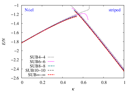
Figure 2: CCM results for the GS energy per spin, $E/N$, for the $J_{1}$–$J_{2}$–$J_{3}$ model on the honeycomb lattice (with $J_{1}\equiv 1,J_{3}=J_{2}\equiv\kappa J_{1}>0$), as a function of $\kappa$, using the Néel and striped states as the CCM model states. (a) The results for the $s=1$ model are shown using the SUB$n$–$n$ approximations with $n=\{4,6,8,10\}$, together with the corresponding extrapolated SUB$\infty$–$\infty$ results obtained using equation (19), with this data set. (b) We show extrapolated (SUB$\infty$–$\infty$) results for $E/(Ns^{2})$ as a function of $\kappa$, using equation (19) together with the data set $n=\{6,8,10,12\}$ for the case $s=\frac{1}{2}$, and the corresponding data sets with $n=\{4,6,8,10\}$ for the four cases $s=1,\,\frac{3}{2},\,2\,,\frac{5}{2}$. We also show the corresponding classical ($s\to\infty$) result.

We observe very clearly that the results converge very rapidly with increasing values of the truncation index $n$, and we also show the extrapolated $n\rightarrow\infty$ results, $a_{0}$, from Eq. (19). We also observe that each of the energy curves based on a particular model state terminates at a critical value of the frustration parameter $\kappa$ that depends on the SUB$n$–$n$ approximation used. Beyond those critical values no real solutions can be found to the corresponding CCM equations (12). Such termination points of the CCM coupled equations are very common in practice, and are well understood (see, e.g., Refs. [16, 50, 62]). They are direct manifestations of the corresponding QCP in the system, at which the respective form of magnetic LRO in the model state used melts. As is usually the case, the CCM SUB$n$–$n$ solutions for a given finite value of $n$ and for a given phase extend beyond the actual SUB$\infty$–$\infty$ QCP, i.e., into the unphysical regime beyond the termination point. The extent of the unphysical regime diminishes (to zero) as the truncation order $n$ increases (to the exact $n\rightarrow\infty$ limit).

In Fig. 2(b) we compare the corresponding extrapolated curves for the scaled GS energy per spin, $E/(Ns^{2})$, using both the Néel and striped AFM states separately as our choice of CCM model state, for the five cases $s=\frac{1}{2},\,1,\,\frac{3}{2},\,2\,,\frac{5}{2}$. In each case the extrapolation is performed with Eq. (19). For the case $s=\frac{1}{2}$ alone the input SUB$n$–$n$ data points are $n=\{6,8,10,12\}$, while for each of the cases $s>\frac{1}{2}$ the input set is $n=\{4,6,8,10\}$. We also show in Fig. 2(b) the corresponding classical ($s\rightarrow\infty$) results, $E^{{\rm N\acute{e}el}}_{{\rm cl}}/(Ns^{2})=\frac{3}{2}(-1+\kappa)$ and $E^{{\rm striped}}_{{\rm cl}}/(Ns^{2})=\frac{1}{2}(1-5\kappa)$. We observe clear preliminary evidence from Fig. 2(b) for an intermediate phase (between the phases with Néel and striped magnetic LRO) in the $s=1$ case, although with a range of stability in the frustration parameter $\kappa$ now markedly less than in the $s=\frac{1}{2}$ case. The preliminary evidence from the energy results is also that there is no such intermediate phase present in each of the cases $s>1$. Lastly, Fig. 2(b) also shows that, at least so far as the energy results are concerned, all cases with $s\gtrsim 2$ are rather close to the classical limit.

In order to get more detailed evidence on the phase structures of the model for various values of the spin quantum number $s$ we now turn to the results for the GS magnetic order parameter, $M$, of Eq. (18). Thus, firstly, in Fig. 3(a) we show our CCM results for $M$ for the spin-1 model at various SUB$n$–$n$ levels of approximation with $n=\{4,6,8,10\}$, using both the Néel and striped AFM states as separate choices for the model state.

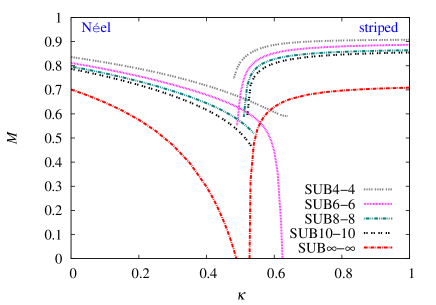
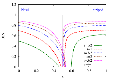
Figure 3: CCM results for the GS magnetic order parameter, $M$, for the $J_{1}$–$J_{2}$–$J_{3}$ model on the honeycomb lattice (with $J_{1}\equiv 1,J_{3}=J_{2}\equiv\kappa J_{1}>0$), as a function of $\kappa$, using the Néel and striped states as the CCM model states. (a) The results for the $s=1$ model are shown using the SUB$n$–$n$ approximations with $n=\{4,6,8,10\}$, together with the corresponding extrapolated SUB$\infty$–$\infty$ results obtained using equation (21), with this data set. (b) We show extrapolated (SUB$\infty$–$\infty$) results for $M/s$ as a function of $\kappa$, using equation (21) together with the data set $n=\{6,8,10,12\}$ for the case $s=\frac{1}{2}$, and the corresponding data sets with $n=\{4,6,8,10\}$ for the four cases $s=1,\,\frac{3}{2},\,2\,,\frac{5}{2}$. We also show the corresponding classical ($s\to\infty$) result.

Hence, what is shown in Fig. 3(a) for $M$ is just the precise analogue of what is shown in Fig. 2(a) for $E/N$. It is clear that the SUB$n$–$n$ sequence of approximations for $M$ converges more slowly than for $E/N$, just as expected. We also show in Fig. 3(a) the extrapolated results for the spin-1 model, where we have used the data set shown, $n=\{4,6,8,10\}$, as input to the extrapolation scheme of Eq. (21). As was explained in Sec. 3, while the alternative scheme of Eq. (20) is certainly more appropriate when the frustration parameter $\kappa$ is zero or small, that of Eq. (21) is certainly preferable for larger values of $\kappa$ (e.g., in the striped phase) or when the order parameter $M$ becomes small (i.e., near any QCPs).

The SUB$\infty$–$\infty$ extrapolation shown in Fig. 3(a) now clearly validates the earlier, more qualitative, results from the GS energy, namely the existence of a GS phase intermediate between the quasiclassical Néel and striped collinear AFM states, just as in the spin-$\frac{1}{2}$ case. Once again, Néel LRO exists over the range $0\leq\kappa<\kappa_{c_{1}}$, while striped LRO exists for $\kappa>\kappa_{c_{2}}$, where $\kappa_{c_{1}}<\kappa_{{\rm cl}}=\frac{1}{2}$ and $\kappa_{c_{2}}>\kappa_{{\rm cl}}=\frac{1}{2}$. The values obtained for the two QCPs from the extrapolations using Eq. (21) with the data set $n=\{4,6,8,10\}$, taken as the points where $M\rightarrow 0$, as shown in Fig. 3(a), are $\kappa_{c_{1}}\approx 0.486$ and $\kappa_{c_{2}}\approx 0.527$. A more detailed analysis of the errors associated with the fits, and by comparison with comparable extrapolations using alternative data sets (e.g., $n=\{6,8,10\}$ and $n=\{4,6,8\}$), yields our best estimates for the spin-1 model QCPs, $\kappa_{c_{1}}=0.485(5)$ and $\kappa_{c_{2}}=0.528(5)$. These may be compared with the corresponding values for the spin-$\frac{1}{2}$ model QCPs [9], $\kappa_{c_{1}}=0.47$ and $\kappa_{c_{2}}=0.60$.

In Fig. 3(b) we now compare the corresponding extrapolated curves for the scaled magnetic order parameter, $M/s$, using both the Néel and striped AFM states separately as CCM model states, for the five cases $s=\frac{1}{2},\,1,\,\frac{3}{2},\,2\,,\frac{5}{2}$. In each case shown the extrapolation has been performed with the ansatz of Eq. (21), together with the data set $n=\{6,8,10,12\}$ for the $s=\frac{1}{2}$ case and the sets $n=\{4,6,8,10\}$ for each case with $s>\frac{1}{2}$. The results once again validate our earlier, more qualitative, findings from the GS energy results, that the intermediate phase is present only for the two cases $s=\frac{1}{2},\,1$, with a direct transition from the Néel to the striped phase in all cases $s>1$, just as in the classical $(s\rightarrow\infty)$ limit. For all cases $s>1$ this direct transition clearly occurs at values very close to the classical value $\kappa_{{\rm cl}}=\frac{1}{2}$. The actual crossing points of the order parameter curves shown in Fig. 3(b) occur at values $\kappa_{m}\approx 0.517$ for $s=\frac{3}{2}$, $\kappa_{m}\approx 0.508$ for $s=2$, and $\kappa_{m}\approx 0.505$ for $s=\frac{5}{2}$. What is apparent from Fig. 3(b) is that the curves for the striped phase approach zero much more steeply than for the Néel phase for all values of $s$. For the case $s=\frac{1}{2}$ it was argued [9] that this was a reflection of the transition at $\kappa_{c_{2}}$ being of first-order type, while that at $\kappa_{c_{1}}$ is of continuous (and hence probably of the deconfined) type. The difference in the shapes of the curves near the crossing point is what leads to the direct transition apparently being at values slightly larger than $\kappa_{{\rm cl}}=\frac{1}{2}$ for finite values of $s>1$.

Clearly the precise crossing points $\kappa_{m}$ of the magnetic order curves for the Néel and striped phases for the cases $s>1$ depend rather critically on the extrapolations, particularly those for the striped phase, where the slope become large. In such cases more precise values of the corresponding QCP for the direct transition between the two quasiclassical phases can be expected to come from the analogous crossing points, $\kappa_{e}$, of the extrapolated energy curves. The respective values from Fig. 2(b) are $\kappa_{e}\approx 0.544$ for $s=\frac{3}{2}$, $\kappa_{e}\approx 0.534$ for $s=2$, and $\kappa_{e}\approx 0.528$ for $s=\frac{5}{2}$. It is reassuring that the respective pairs of values of $\kappa_{e}$ and $\kappa_{m}$ agree so well in each case, for what are essentially quite independent results.

Before discussing how we can investigate the nature of the intermediate phase for the present $s=1$ case within the CCM framework, let us briefly comment on the case of the pure HAF on the honeycomb lattice, with NN interactions only (i.e., the limiting case $\kappa=0$ of the present model). In this case, the extrapolation ansatz of Eq. (20) becomes applicable, rather than that of Eq. (21) shown in Fig. 3. We show in Table 1 the scaled values for the GS energy per spin and magnetic order parameters, $E/(Ns^{2})$ and $M/s$, respectively, for our present model calculations at the unfrustrated limiting value $\kappa=0$.

Table 1: GS parameters of the HAF on the honeycomb lattice, with NN interactions only (of strength $J_{1}=1$), for various values of the spin quantum number $s$.

$s$	$E/(Ns^{2})$	$M/s$
$\frac{1}{2}$	-2.17866	0.5459
1	-1.83061	0.7412
$\frac{3}{2}$	-1.71721	0.8249
2	-1.66159	0.8689
$\frac{5}{2}$	-1.62862	0.8955
$\infty$	-1.5	1

The corresponding extrapolation schemes of Eqs. (19) and Eq. (20) have been used in Table 1, together with the input data sets with $n=\{6,8,10,12\}$ for $s=\frac{1}{2}$, and with $n=\{4,6,8,10\}$ for $s>\frac{1}{2}$.

Another way to estimate the accuracy of our extrapolated CCM results for the higher spin values is to use them to extract, for example, the coefficients of the expansions of $E/(Ns^{2})$ and $M/s$ in inverse powers of $s$, and compare them with the results of higher-order spin-wave theory (SWT). For example, at second-order, we may fit our results of Table 1 to the forms,

$$\frac{E}{Ns^{2}}=-\frac{3}{2}+\frac{e_{1}}{s}+\frac{e_{2}}{s^{2}}\,,$$ (22)

and

$$\frac{M}{s}=1+\frac{m_{1}}{s}+\frac{m_{2}}{s^{2}}\,,$$ (23)

and then compare with the corresponding results of second-order SWT, i.e., SWT(2). If we simply take our results from Table 1 for the two highest spin values calculated, viz., $s=2,\,\frac{5}{2}$, and fit them to Eqs. (22) and (23), we obtain values $e_{1}\approx-0.31503$ and $e_{2}\approx-0.01630$ for the GS energy, and $m_{1}\approx-0.2575$ and $m_{2}\approx-0.0095$ for the GS Néel magnetic order parameter (i.e., the sublattice magnetization). The corresponding (exact) SWT(2) results [68] are $e_{1}=-0.31476$, $e_{2}=-0.01651$, $m_{1}=-0.2582$, and $m_{2}=0$. The agreement is rather striking.

We now turn finally to the question of what is the nature of the intermediate phase in the case $s=1$. For the analogous $s=\frac{1}{2}$ case it was shown [9] that the intermediate paramagnetic phase likely had PVBC order. It is natural now to consider this possibility for the $s=1$ case. To do so we now calculate within the CCM framework the susceptibility, $\chi_{p}$, which measures the response of the system to an applied external field that promotes PVBC order. More generally, let us add an infinitesimal field operator $F\equiv\delta\;\hat{O}$ to the Hamiltonian $H$ of Eq. (1). We then calculate the perturbed energy per site, $E(\delta)/N=e(\delta)$, for the perturbed Hamiltonian $H+F$, using the same CCM procedure as above, and using the same previous model states. The susceptibility of the system to the perturbed operator $\hat{O}$ is then defined as usual to be

$$\chi_{F}\equiv-\left.\frac{\partial^{2}e(\delta)}{\partial{\delta}^{2}}\right|_{\delta=0\,,}$$ (24)

so that the energy,

$$e(\delta)=e(0)-\frac{1}{2}\chi_{F}\delta^{2}\,,$$ (25)

is a maximum at $\delta=0$ for $\chi_{F}>0$. A clear signal of the system becoming unstable against the perturbation $F$ is the finding that $\chi_{F}$ diverges or, equivalently, that $\chi_{F}^{-1}$ becomes zero (and then possibly changes sign).

In our present case the perturbing operator $F$ is now chosen to promote PVBC order, and it is illustrated in Fig. 4(a).

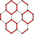
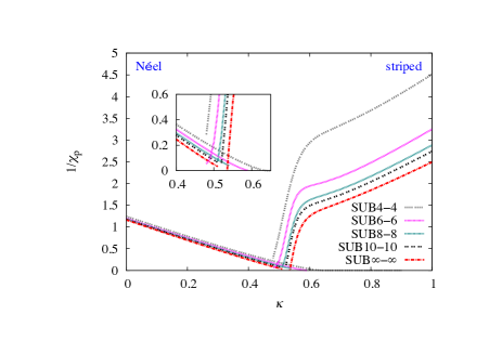
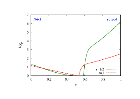
Figure 4: (a) The fields $F=\delta\;\hat{O}$ for the plaquette susceptibility $\chi_{p}$. Thick (red) and thin (black) lines correspond respectively to strengthened and weakened NN exchange couplings, where $\hat{O}=\sum_{\langle i,j\rangle}a_{ij}\mathbf{s}_{i}\cdot\mathbf{s}_{j}$, and the sum runs over all NN bonds, with $a_{ij}=+1$ and $-1$ for thick (red) and thin (black) lines respectively. (b) CCM results for the inverse plaquette susceptibility, $1/\chi_{p}$, for the $J_{1}$–$J_{2}$–$J_{3}$ model on the honeycomb lattice (with $J_{1}\equiv 1,J_{3}=J_{2}\equiv\kappa J_{1}>0$), as a function of $\kappa$, using the Néel and striped states as the CCM model states. The results for the $s=1$ model are shown using the SUB$n$–$n$ approximations with $n=\{4,6,8,10\}$, together with the corresponding extrapolated SUB$\infty$–$\infty$ results obtained using equation (26), with this data set. (c) We show extrapolated (SUB$\infty$–$\infty$) results for $1/\chi_{p}$ as a function of $\kappa$, using equation (26) together with the data set $n=\{6,8,10,12\}$ for the case $s=\frac{1}{2}$, and the data set $n=\{4,6,8,10\}$ for the case $s=1$.

It clearly breaks the translational symmetry of the system. The SUB$n$–$n$ estimates, $\chi_{p}(n)$, for the resulting susceptibility of our system to the formation of PVBC order, then need to be extrapolated to the exact ($n\rightarrow\infty$) limit. Previous experience [9] has shown that an appropriate extrapolation ansatz is

$$\chi_{p}^{-1}(n)=x_{0}+x_{1}n^{-2}+x_{2}n^{-4}\,.$$ (26)

We show in Fig. 4(b) our CCM results for $\chi_{p}^{-1}(n)$ at SUB$n$–$n$ levels of approximation with $n=\{4,6,8,10\}$, using both the Néel and striped AFM states separately as model states, in complete analogy to what is displayed in Figs. 2(a) and 3(a) for the GS energy per spin, $E/N$, and magnetic order parameter, $M$. In Fig. 4(b) we also show the extrapolated results ($x_{0}$) obtained by inserting the set of raw results shown into Eq. (26). Just as in the spin-$\frac{1}{2}$ case [9], the results for $\chi_{p}^{-1}(n)$ converge much faster for the Néel state than for the striped state. For both states there are clear critical points at which $\chi_{p}^{-1}$ vanishes. However, the shapes of the curves for $\chi_{p}^{-1}$ near their respective critical points differ markedly, just as in the spin-$\frac{1}{2}$ case. Thus, on the Néel side, $\chi_{p}^{-1}\rightarrow 0$ with a slope that is small. By contrast, on the striped side, $\chi_{p}^{-1}\rightarrow 0$ with a very large slope (and which is probably compatible with being infinite, within extrapolation errors). These differences reinforce our earlier findings that the critical point at which Néel order vanishes is likely to mark a continuous phase transition, while that at which striped order vanishes is likely to mark a first-order transition.

In Fig. 4(c) we compare the extrapolated CCM results for $\chi_{p}^{-1}$ for the two cases ($s=\frac{1}{2},\,1$) for which our findings indicate the existence in the model of a phase in its $T=0$ GS phase diagram intermediate between the two quasiclassical phases with magnetic LRO. Whereas in the spin-$\frac{1}{2}$ case there exists a clear gap along the frustration parameter, $\kappa$, axis between the two points at which $\chi_{p}^{-1}$ vanishes (one for each quasiclassical phase), the gap in the spin-1 case is much less marked. Indeed, its very existence is open to doubt, as we explain below. For the spin-$\frac{1}{2}$ case [9] the two values on Fig. 4(c) at which $\chi_{p}^{-1}\rightarrow 0$ are $\kappa\approx 0.473$ and $\kappa\approx 0.586$. These may be compared with the corresponding values on Fig. 3(b) at which $M\rightarrow 0$, which are $\kappa_{c_{1}}\approx 0.466$ and $\kappa_{c_{2}}\approx 0.601$. The very close agreement between the corresponding values was taken [9] to be good evidence that the PVBC phase occurs at (or is very close to) the transition points $\kappa_{c_{1}}$ and $\kappa_{c_{2}}$ where the quasiclassical magnetic LRO vanishes. The fact that the slope of the $\chi_{p}^{-1}(\kappa)$ curve on the Néel side is vanishingly small (within numerical errors) at the point where $\chi_{p}^{-1}\rightarrow 0$, also provided strong evidence that $\chi_{p}^{-1}$ vanishes over the entire intermediate region in Fig. 4(c) between the points, where the CCM calculations have been performed with the two classical model states. All of this evidence pointed strongly to the stable GS phase in the whole of the region $\kappa_{c_{1}}<\kappa<\kappa_{c_{2}}$ being one with PVBC order, in the $s=\frac{1}{2}$ case. If any other phase exists in part of this region, its region of stability is clearly constrained by the CCM calculations [9] to be a very small part of the intermediate region.

The corresponding situation for the $s=1$ case is now subtly different, however. Thus, firstly, a close inspection of Fig. 4(b) (and, especially, the inset) shows that on the Néel side the extrapolated SUB$\infty$–$\infty$ $\chi_{p}^{-1}(\kappa)$ curve has not quite reached zero at the SUB10–10 termination point (or at least as far as we have managed to perform numerical calculations, which, as we discussed above, become increasingly difficult and computationally costly the closer one approaches a termination point). A simple further extrapolation of the curve, however, yields a value $\kappa\approx 0.530(2)$ at which $\chi_{p}^{-1}\rightarrow 0$ on the Néel side. This is very close to the corresponding value in Fig. 4(b) of $\kappa\approx 0.535$ at which $\chi_{p}^{-1}\rightarrow 0$ on the striped phase side. Significantly, both of these values are indubitably greater than $\kappa_{{\rm cl}}=\frac{1}{2}$. By contrast, the corresponding values from Fig. 3(b) at which $M\rightarrow 0$ for the spin-1 model are $\kappa_{c_{1}}\approx 0.486$ and $\kappa_{c_{2}}\approx 0.527$. The most likely interpretation of our $\chi_{p}$ results is hence that the CCM using both model states is showing that $\chi_{p}^{-1}$ vanishes only at a single point, viz., the QCP $\kappa_{c_{2}}$, for the spin-1 model. This interpretation is lent further weight by the observation that, unlike in the spin-$\frac{1}{2}$ case, the slope of the $\chi_{p}^{-1}(\kappa)$ curve on the Néel side does not appear to be zero at the (extrapolated) point at which it becomes zero.

In summary, if a PVBC-ordered phase is stable anywhere in the intermediate regime $\kappa_{c_{1}}<\kappa<\kappa_{c_{2}}$, our findings are that it is confined only to a very narrow range close to $\kappa_{c_{2}}$, and that it is definitely not the stable GS phase over the whole interval. The more likely scenario is that the intermediate regime is occupied by a paramagnetic phase (or more than one such phase) with a form of order other than PVBC.

5 Conclusions

We have investigated higher-spin versions of a frustrated $J_{1}$–$J_{2}$–$J_{3}$ HAF model on the honeycomb lattice, in the specific case where $J_{1}>0$, $J_{3}=J_{2}\equiv\kappa J_{1}>0$, over the range $0\leq\kappa\leq 1$ of the frustration parameter. This includes the point of maximum frustration in the classical ($s\rightarrow\infty$) limit, viz., the tricritical point at $\kappa_{{\rm cl}}=\frac{1}{2}$, at which there is a direct first-order transition (along the line $J_{3}=J_{2}$) between a Néel-ordered AFM phase for $\kappa<\kappa_{{\rm cl}}$ and a collinear stripe-ordered AFM phase for $\kappa>\kappa_{{\rm cl}}$. Whereas the spin-$\frac{1}{2}$ version of the model has been studied previously, higher-spin versions have received no attention, so far as we are aware.

In particular, the CCM has been applied to the spin-$\frac{1}{2}$ model in an earlier study [9] that yielded accurate results for its entire $T=0$ GS phase diagram. Since the method generally provides values for the QCPs of a wide range of spin-lattice systems, which are among the most accurate available by any alternative methodology, we have now used the CCM to study spin-$s$ versions of the model with values of the spin quantum number $s>\frac{1}{2}$. An aim has been to compare the $T=0$ GS phase diagrams of the higher-spin models with the two extreme limits, $s=\frac{1}{2}$ (where quantum effects should be greatest) and $s\rightarrow\infty$ (where quantum effects vanish). In particular, it has been shown [9] that the direct classical transition at $\kappa_{{\rm cl}}=\frac{1}{2}$ is split by quantum fluctuations in the spin-$\frac{1}{2}$ model into two separate transitions at $\kappa_{c_{1}}<\kappa_{{\rm cl}}$ and $\kappa_{c_{2}}>\kappa_{{\rm cl}}$, at the first of which Néel AFM order of the type shown in Fig. 1(a) breaks down, and at the second of which striped AFM order of the type shown in Fig. 1(b) breaks down. Between the regimes $\kappa<\kappa_{c_{1}}$ in which the stable GS phase has Néel magnetic LRO and $\kappa>\kappa_{c_{2}}$ in which the stable GS phase has striped magnetic LRO, there opens an intermediate paramagnetic regime $\kappa_{c_{1}}<\kappa<\kappa_{c_{2}}$. Strong evidence was presented [9] that the stable GS phase in this entire intermediate regime in the spin-$\frac{1}{2}$ case is an intrinsically quantum-mechanical one with PVBC order.

We have now performed analogous CCM calculations for spin-$s$ versions of the same honeycomb lattice model for values $s=1,\,\frac{3}{2},\,2\,,\frac{5}{2}$. A primary finding is that an intermediate phase also exists for the case $s=1$, but that for all higher spins ($s\geq\frac{3}{2}$) the intermediate phase disappears in favour of a direct transition between the two quasiclassical states with magnetic LRO. For all finite values of the spin quantum number $s\geq\frac{3}{2}$ the direct transition seems to occur at a value $\kappa_{c}$ marginally higher than the classical value of 0.5 [e.g., for $s=\frac{3}{2}$, $\kappa_{c}\approx 0.53(1)$, and for $s=\frac{5}{2}$, $\kappa_{c}\approx 0.52(1)$], with $\kappa_{c}$ tending monotonically to 0.5 as $s\rightarrow\infty$.

The range of the intermediate phase is smaller for the spin-1 model ($\kappa_{c_{1}}\approx 0.49$, $\kappa_{c_{2}}\approx 0.53$) than for its spin-$\frac{1}{2}$ counterpart ($\kappa_{c_{1}}\approx 0.47$, $\kappa_{c_{2}}\approx 0.60$), as expected. Interestingly, all of the evidence garnered here is that, unlike in the spin-$\frac{1}{2}$ case the intermediate phase for the spin-1 model does not have PVBC ordering. On the other hand, both the spin-$\frac{1}{2}$ and spin-1 models seem to share that the transition at $\kappa_{c_{2}}$ is a direct first-order one while that at $\kappa_{c_{1}}$ is continuous.

On the basis of the present calculations, the nature and properties of the intermediate phase in the spin-1 version of the model remain open questions. It will be of considerable interest to study this phase further, both by the CCM and by the use of alternative techniques. A particularly promising such alternative technique in this respect is the DMRG method, which has been used very recently [25] in an analysis of the quantum ($T=0$) phase diagram of the spin-1 version of the related $J_{1}$–$J_{2}$ Heisenberg model on the honeycomb lattice.

References

References

- [1] Mermin N D and Wagner H 1966 Phys. Rev. Lett. 17 1133
- [2] Rastelli E, Tassi A and Reatto L 1979 Physica B & C 97 1
- [3] Fouet J B, Sindzingre P and Lhuillier C 2001 Eur. Phys. J. B 20 241
- [4] Cabra D C, Lamas C A and Rosales H D 2011 Phys. Rev. B 83 094506
- [5] Mattsson A, Fröjdh P and Einarsson T 1994 Phys. Rev. B 49 3997–4002
- [6] Mulder A, Ganesh R, Capriotti L and Paramekanti A 2010 Phys. Rev. B 81 214419
- [7] Ganesh R, Sheng D N, Kim Y J and Paramekanti A 2011 Phys. Rev. B 83 144414
- [8] Clark B K, Abanin D A and Sondhi S L 2011 Phys. Rev. Lett. 107 087204
- [9] Farnell D J J, Bishop R F, Li P H Y, Richter J and Campbell C E 2011 Phys. Rev. B 84 012403
- [10] Reuther J, Abanin D A and Thomale R 2011 Phys. Rev. B 84 014417
- [11] Albuquerque A F, Schwandt D, Hetényi B, Capponi S, Mambrini M and Läuchli A M 2011 Phys. Rev. B 84 024406
- [12] Mosadeq H, Shahbazi F and Jafari S A 2011 J. Phys.: Condens. Matter 23 226006
- [13] Oitmaa J and Singh R R P 2011 Phys. Rev. B 84 094424
- [14] Mezzacapo F and Boninsegni M 2012 Phys. Rev. B 85 060402(R)
- [15] Li P H Y, Bishop R F, Farnell D J J, Richter J and Campbell C E 2012 Phys. Rev. B 85 085115
- [16] Bishop R F, Li P H Y, Farnell D J J and Campbell C E 2012 J. Phys.: Condens. Matter 24 236002
- [17] Bishop R F and Li P H Y 2012 Phys. Rev. B 85 155135
- [18] Li P H Y, Bishop R F, Farnell D J J and Campbell C E 2012 Phys. Rev. B 86 144404
- [19] Bishop R F, Li P H Y and Campbell C E 2013 J. Phys.: Condens. Matter 25 306002
- [20] Ganesh R, van den Brink J and Nishimoto S 2013 Phys. Rev. Lett. 110 127203
- [21] Zhu Z, Huse D A and White S R 2013 Phys. Rev. Lett. 111 257201
- [22] Zhang H and Lamas C A 2013 Phys. Rev. B 87 024415
- [23] Gong S S, Sheng D N, Motrunich O I and Fisher M P A 2013 Phys. Rev. B 88 165138
- [24] Yu X L, Liu D Y, Li P and Zou L J 2014 Physica E 59 41
- [25] Gong S S, Zhu W and Sheng D N 2015 Quantum phase diagram of the spin-1 – Heisenberg model on the honeycomb lattice arXiv:1508.00515
- [26] Miura Y, Hirai R, Kobayashi Y and Sato M 2006 J. Phys. Soc. Jpn. 75 084707
- [27] Kataev V, Möller A, Löw U, Jung W, Schittner N, Kriener M and Freimuth A 2005 J. Magn. Magn. Mater. 290–291 310–313
- [28] Tsirlin A A, Janson O and Rosner H 2010 Phys. Rev. B 82 144416
- [29] Climent-Pascual E, Norby P, Andersen N, Stephens P, Zandbergen H, Larsen J and Cava R 2012 Inorg. Chem. 51 557–565
- [30] Singh Y and Gegenwart P 2010 Phys. Rev. B 82 064412
- [31] Liu X, Berlijn T, Yin W G, Ku W, Tsvelik A, Kim Y J, Gretarsson H, Singh Y, Gegenwart P and Hill J P 2011 Phys. Rev. B 83 220403(R)
- [32] Singh Y, Manni S, Reuther J, Berlijn T, Thomale R, Ku W, Trebst S and Gegenwart P 2012 Phys. Rev. Lett. 108 127203
- [33] Choi S K, Coldea R, Kolmogorov A N, Lancaster T, Mazin I I, Blundell S J, Radaelli P G, Singh Y, Gegenwart P, Choi K R, Cheong S W, Baker P J, Stock C and Taylor J 2012 Phys. Rev. Lett. 108 127204
- [34] Regnault L P and Rossat-Mignod J 1990 Magnetic properties of layered transition metal compounds ed De Jongh L J (Dordrecht: Kluwer Academic Publishers) pp 271–321
- [35] Roudebush J H, Andersen N H, Ramlau R, Garlea V O, Toft-Petersen R, Norby P, Schneider R, Hay J N and Cava R J 2013 Inorg. Chem. 52 6083–6095
- [36] Smirnova O, Azuma M, Kumada N, Kusano Y, Matsuda M, Shimakawa Y, Takei T, Yonesaki Y and Kinomura N 2009 J. Am. Chem. Soc. 131 8313–8317
- [37] Okubo S, Elmasry F, Zhang W, Fujisawa M, Sakurai T, Ohta H, Azuma M, Sumirnova O A and Kumada N 2010 J. Phys.: Conf. Ser. 200 022042
- [38] Villain J 1977 J. Phys. (France) 38 385
- [39] Villain J, Bidaux R, Carton J P and Conte R 1980 J. Phys. (France) 41 1263
- [40] Shender E F 1982 Zh. Eksp. Teor. Fiz. 83 326–337
- [41] Senthil T, Vishwanath A, Balents L, Sachdev S and Fisher M P A 2004 Science 303 1490
- [42] Senthil T, Balents L, Sachdev S, Vishwanath A and Fisher M P A 2004 Phys. Rev. B 70 144407
- [43] Bishop R F and Lührmann K H 1978 Phys. Rev. B 17 3757–3780
- [44] Bishop R F and Lührmann K H 1982 Phys. Rev. B 26 5523–5557
- [45] Arponen J 1983 Ann. Phys. (N.Y.) 151 311–382
- [46] Bishop R F and Kümmel H G 1987 Phys. Today 40(3) 52
- [47] Arponen J S and Bishop R F 1991 Ann. Phys. (N.Y.) 207 171
- [48] Bishop R F 1991 Theor. Chim. Acta 80 95
- [49] Bishop R F 1998 Microscopic Quantum Many-Body Theories and Their Applications Lecture Notes in Physics Vol. 510 ed Navarro J and Polls A (Berlin: Springer-Verlag) p 1
- [50] Farnell D J J and Bishop R F 2004 Quantum Magnetism Lecture Notes in Physics Vol. 645 ed Schollwöck U, Richter J, Farnell D J J and Bishop R F (Berlin: Springer-Verlag) p 307
- [51] Bartlett R J 1989 J. Phys. Chem. 93 1697
- [52] Kümmel H, Lührmann K H and Zabolitzky J G 1978 Phys Rep. 36C 1
- [53] Zeng C, Farnell D J J and Bishop R F 1998 J. Stat. Phys. 90 327
- [54] We use the program package CCCM of D. J. J. Farnell and J. Schulenburg, see http://www-e.uni-magdeburg.de/jschulen/ccm/index.html
- [55] Bishop R F, Farnell D J J, Krüger S E, Parkinson J B, Richter J and Zeng C 2000 J. Phys.: Condens. Matter 12 6887
- [56] Krüger S E, Richter J, Schulenburg J, Farnell D J J and Bishop R F 2000 Phys. Rev. B 61 14607
- [57] Farnell D J J, Gernoth K A and Bishop R F 2001 Phys. Rev. B 64 172409
- [58] Darradi R, Richter J and Farnell D J J 2005 Phys. Rev. B 72 104425
- [59] Darradi R, Derzhko O, Zinke R, Schulenburg J, Krüger S E and Richter J 2008 Phys. Rev. B 78 214415
- [60] Bishop R F, Li P H Y, Darradi R and Richter J 2008 Europhys. Lett. 83 47004
- [61] Bishop R F, Li P H Y, Darradi R, Richter J and Campbell C E 2008 J. Phys.: Condens. Matter 20 415213
- [62] Bishop R F, Li P H Y, Farnell D J J and Campbell C E 2009 Phys. Rev. B 79 174405
- [63] Bishop R F, Li P H Y, Farnell D J J and Campbell C E 2010 Phys. Rev. B 82 024416
- [64] Bishop R F, Li P H Y, Farnell D J J and Campbell C E 2010 Phys. Rev. B 82 104406
- [65] Bishop R F and Li P H Y 2011 Eur. Phys. J. B 81 37
- [66] Li P H Y and Bishop R F 2012 Eur. Phys. J. B 85 25
- [67] Li P H Y, Bishop R F, Campbell C E, Farnell D J J, Götze O and Richter J 2012 Phys. Rev. B 86 214403
- [68] Weihong Z, Oitmaa J and Hamer C J 1991 Phys. Rev. B 44 11869–11881