Experimental demonstration of quantum contextuality on an NMR qutrit

Abstract

We experimentally test quantum contextuality of a single qutrit using NMR. The contextuality inequalities based on nine observables developed by Kurzynski et. al. are first reformulated in terms of traceless observables which can be measured in an NMR experiment. These inequalities reveal the contextuality of almost all single-qutrit states. We demonstrate the violation of the inequality on four different initial states of a spin-1 deuterium nucleus oriented in a liquid crystal matrix, and follow the violation as the states evolve in time. We also describe and experimentally perform a single-shot test of contextuality for a subclass of qutrit states whose density matrix is diagonal in the energy basis.

I Introduction

The existence of contextuality in the quantum description of physical reality is a fundamental departure from any classical theory. For classical systems, a joint probability distribution exists for the results of any set of joint measurements on the system, and the results of a measurement of a variable do not depend on the measurements of other compatible variables. In non-contextual hidden variable theories, one can hence pre-assign the values to measurement outcomes of observables before the measurement is actually performed Peres (1993). Quantum mechanics on the other hand, precludes such a description of physical reality. In quantum mechanics there exists a context among the measurement outcomes, which forbids us from arriving at joint probability distributions of more than two observables. Given observables $A$, $B$ and $C$, such that $A$ commutes with both $B$ and $C$, while $[B,C]\neq 0$; a measurement of $A$ along with $B$ and a measurement of $A$ along with $C$, may lead to different measurement outcomes for $A$. Thus, to be able to make quantum mechanical predictions about the outcome of a measurement, the context of the measurement needs to be specified.

The first test for contextuality was proposed by Kochen and Specker Kochen and Specker (1967), wherein they used a set of 117 rays to reveal the contextuality of a single qutrit (the KS theorem). A modified KS scheme based on 33 rays was constructed by Peres Peres (1991). Since then, there have been various proposals to reduce the number of observables required to demonstrate quantum contextuality. For state-dependent contextuality tests, only a subset of quantum states show contextuality while other measurements can be explained by deterministic noncontextual hidden variable models Klyachko et al. (2008). State-independent contextuality tests can be represented by an orthogonality graph Cabello et al. (2015). A state-independent test of quantum contextuality on a qutrit using a set of thirteen projectors was developed Yu and Oh (2012) and was later proved to be optimal Cabello et al. (2012). Kurzynski et. al. Kurzynski and Kaszlikowski (2012) showed that in the case of a qutrit, a contextuality test based on a set of nine measurements is able to reveal the contextuality of all single-qutrit states except the maximally mixed state (which saturates their constructed inequality). More recent studies have focused on testing the contextuality of indistinguishable particles and mixed qutrit states Su et al. (2015); Xu et al. (2015).

Experimental implementations of contextuality tests have been performed by different groups using photonic qutrits Zu et al. (2012); Thompson et al. (2013); Huang et al. (2013). KS inequalities on qubits have been tested experimentally using a solid-state ensemble NMR quantum computer Moussa et al. (2010). Hardy-like quantum contextuality has been experimentally observed by performing sequential measurements on photons Marques et al. (2014). Furthermore, the connection of contextuality with computational speedup via magic state distillation has been explored Howard et al. (2014), and the use of a single qutrit as a quantum computational resource has also been experimentally demonstrated Dogra et al. (2014); Gedik et al. (2015).

In the current paper, we experimentally demonstrate the contextuality of a qutrit using NMR. On the basis of a set of nine measurements, an experimental test for contextuality is designed and implemented on an NMR qutrit. This involves recasting the original Kurzynski inequality Kurzynski and Kaszlikowski (2012) in terms of traceless observables, which can be measured in an NMR experiment. The Gell-Mann matrices provide a natural set to be used in this new scheme, as they are traceless and hence measurable by NMR. We use a deuterium nucleus (spin-1) oriented in a liquid crystalline environment as the NMR qutrit, with the effective quadrupole moment of the spin contributing to two non-overlapping resonances in the NMR spectrum at thermal equilibrium.

The material in this paper is arranged as follows: Section II describes the single-qutrit state-independent contextuality inequality and the reformulation of this inequality in terms of an experimentally feasible set of measurements in NMR. Section III presents the experimental implementation of single-qutrit contextuality, and Section IV contains a few concluding remarks.

II State-independent test with nine observables

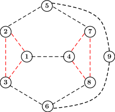
Figure 1: An orthogonality graph $G$ with the nine projectors as the vertices and the edges $E(G)$ denoting the orthogonality relations between different vertices. An edge between two vertices indicates that the corresponding projectors are orthogonal.

The contextuality test for a single qutrit proposed by Kurzynski et. al. Kurzynski and Kaszlikowski (2012), consists of nine measurements that can reveal the contextuality of all single-qutrit states (other than the maximally mixed state represented by the identity density operator). The set of nine projectors are represented as

$$\Pi_{i}=|\psi_{i}\rangle\langle\psi_{i}|,\quad i=1,2\cdots 9.$$ (1)

The vectors $|\psi_{i}\rangle$ occupy vertices in the orthogonality graph $G$ and the edges connect the vertices occupied by mutually orthogonal vectors as shown in Fig. 1.

As per non-contextual hidden variable theories, one can consider a pre-assignment of the dichotomous measurement outcomes ($0$ or $1$) to each of the projection operators $\Pi_{i}$. The projection operators obey the orthogonality relations depicted in Graph $G$, due to which no two connected vertices in Graph $G$ can simultaneously be assigned the value $1$. Thus the sum total of the maximum value of the measurement outcomes that can be obtained from Graph $G$ is $3$. Therefore, repeated projective measurements of $\Pi_{i}$ over an ensemble of identically prepared single qutrit states yields the following inequality:

$$\sum_{i=1}^{9}\langle\Pi_{i}\rangle\leq 3.$$ (2)

Introducing dichotomous observables $A_{i}=I-2\Pi_{i}$ with eigen values $\pm 1$ associated with projection operators $\Pi_{i}$ and by using the inequality in (2) we obtain

$$\quad\sum_{i=1}^{9}\langle A_{i}\rangle\geq 3.$$ (3)

Measurement outcomes of $A_{i}$ and $A_{j}$ which are connected to each other by an edge in the graph G are mutually exclusive and can be measured simultaneously. The edge can be thought of as defining a context, and each $A_{i}$ occurs in more than one context.

Pre-assignment of the measurement outcomes to each of these observables on the basis of a non-contextual hidden variable theory, does not consider the joint probability distributions of all those operators which are being co-measured. Considering the non-contextual pre-assignments (as before),  (2) is reformulated in terms of the contexts, represented as the correlations between the compatible observables $A_{i},A_{j}$ sharing an edge and leads to the following inequality:

$$\sum_{i,j\in E(G)}\langle A_{i}A_{j}\rangle+\langle A_{9}\rangle\geq-4$$ (4)

The inequalities in (2) and (3) represent single-qutrit contextuality inequalities in terms of the set of nine measurements and (4) represents the contextuality inequality based on contexts defined in the graph G. The violation of these inequalities indicates the contextual nature of a single-qutrit state and can be experimentally tested by performing repeated measurements of operators $A_{i}$ on an ensemble of identically prepared qutrit states. There is no unique set of nine measurements that test the contextual nature of every single-qutrit state. However, corresponding to every single-qutrit state (except the maximally mixed state), one can always find a set of nine projectors that reveal its contextuality Kurzynski and Kaszlikowski (2012).

II.1 Reformulation of contextuality inequalities in terms of traceless operators

In this subsection we turn to constructing tests to verify qutrit contextuality on an NMR quantum information processor. Since, in NMR we can measure only traceless observables, we need to reformulate the inequalities developed in  (2),(3) and (4) in terms of traceless observables. A natural set of traceless observables is provided by the eight Gell-Mann or $\Lambda$ matrices Gell-Mann and Neeman (1964) and they have been used for qutrit analysis earlier Arvind et al. (1997). In the basis spanned by the eigen states of $S_{z}$, namely the states $\{|+1\rangle,|0\rangle,|-1\rangle\}$ (which we will follow in the rest of this paper), these matrices are given by:

$$\Lambda_{1}=\left(\begin{array}[]{ccc}0&1&0\\ 1&0&0\\ 0&0&0\end{array}\right)\Lambda_{2}=\left(\begin{array}[]{ccc}0&-\iota&0\\ \iota&0&0\\ 0&0&0\end{array}\right)\Lambda_{3}=\left(\begin{array}[]{ccc}1&0&0\\ 0&-1&0\\ 0&0&0\end{array}\right)$$ (14)

$$\Lambda_{4}=\left(\begin{array}[]{ccc}0&0&1\\ 0&0&0\\ 1&0&0\end{array}\right)\Lambda_{5}=\left(\begin{array}[]{ccc}0&0&-\iota\\ 0&0&0\\ \iota&0&0\end{array}\right)\Lambda_{6}=\left(\begin{array}[]{ccc}0&0&0\\ 0&0&1\\ 0&1&0\end{array}\right)$$ (24)

$$\Lambda_{7}=\left(\begin{array}[]{ccc}0&0&0\\ 0&0&-\iota\\ 0&\iota&0\end{array}\right)\quad\Lambda_{8}=\frac{1}{\sqrt{3}}\left(\begin{array}[]{ccc}1&0&0\\ 0&1&0\\ 0&0&-2\end{array}\right)$$ (31)

At this stage we make a choice of a particular set of nine vectors $|\psi_{j}\rangle,j=1\cdots 9$, occupying the vertices of the graph G in Figure 1. The vectors that we choose are given in the $S_{z}$ basis as:

$$|\psi_{1}\rangle=\left(\begin{array}[]{c}1\\ 0\\ 0\end{array}\right),|\psi_{2}\rangle=\left(\begin{array}[]{c}0\\ 1\\ 0\end{array}\right),|\psi_{3}\rangle=\left(\begin{array}[]{c}0\\ 0\\ 1\end{array}\right),$$ (41)

$$|\psi_{4}\rangle=\left(\begin{array}[]{c}0\\ \sqrt{\frac{1}{2}}\\ -\sqrt{\frac{1}{2}}\end{array}\right),|\psi_{5}\rangle=\left(\begin{array}[]{c}\sqrt{\frac{1}{3}}\\ 0\\ -\sqrt{\frac{2}{3}}\end{array}\right),|\psi_{6}\rangle=\left(\begin{array}[]{c}\sqrt{\frac{1}{3}}\\ \sqrt{\frac{2}{3}}\\ 0\end{array}\right),$$ (51)

$$|\psi_{7}\rangle=\left(\begin{array}[]{c}\sqrt{\frac{1}{2}}\\ \frac{1}{2}\\ \frac{1}{2}\end{array}\right),|\psi_{8}\rangle=\left(\begin{array}[]{c}\sqrt{\frac{1}{2}}\\ -\frac{1}{2}\\ -\frac{1}{2}\end{array}\right),|\psi_{9}\rangle=\left(\begin{array}[]{c}\sqrt{\frac{1}{2}}\\ -\frac{1}{2}\\ \frac{1}{2}\end{array}\right)$$ (61)

The observables corresponding to the nine projection operators $A_{i}$ for this specific case can be written as a combination of a set of eight $\Lambda$ matrices and the identity matrix $I$:

$$A_{1} = -\Lambda_{3}-\frac{1}{\sqrt{3}}\Lambda_{8}+\frac{I}{3}$$

$$A_{2} = \Lambda_{3}-\frac{1}{\sqrt{3}}\Lambda_{8}+\frac{I}{3}$$

$$A_{3} = \frac{2}{\sqrt{3}}\Lambda_{8}+\frac{I}{3}$$

$$A_{4} = \frac{1}{2}\left(\Lambda_{3}+2\Lambda_{6}+\frac{\Lambda_{8}}{\sqrt{3}}\right)+\frac{I}{3}$$

$$A_{5} = \frac{1}{3}\left(-\Lambda_{3}+2\sqrt{2}\Lambda_{4}+\sqrt{3}\Lambda_{8}\right)+\frac{I}{3}$$

$$A_{6} = \frac{1}{3}\left(-2\sqrt{2}\Lambda_{1}+\Lambda_{3}-\sqrt{3}\Lambda_{8}\right)+\frac{I}{3}$$

$$A_{7} = \frac{1}{4}\left(-2\sqrt{2}\Lambda_{1}-\Lambda_{3}-2\sqrt{2}\Lambda_{4}-2\Lambda_{6}-\frac{\Lambda_{8}}{\sqrt{3}}\right)+\frac{I}{3}$$

$$A_{8} = \frac{1}{4}\left(2\sqrt{2}\Lambda_{1}-\Lambda_{3}+2\sqrt{2}\Lambda_{4}-2\Lambda_{6}-\frac{\Lambda_{8}}{\sqrt{3}}\right)+\frac{I}{3}$$

$$A_{9} = \frac{1}{4}\left(2\sqrt{2}\Lambda_{1}-\Lambda_{3}-2\sqrt{2}\Lambda_{4}+2\Lambda_{6}-\frac{\Lambda_{8}}{\sqrt{3}}\right)+\frac{I}{3}$$

Substituting these in the inequality in (3) we obtain:

$$\langle-2\sqrt{2}\Lambda_{1}-3\Lambda_{3}+2\sqrt{2}\Lambda_{4}+6\Lambda_{6}-\sqrt{3}\Lambda_{8}\rangle\geq 0$$ (63)

which is an inequality written in terms of traceless observables and obeyed by any non-contextual single qutrit state. For a contextual single-qutrit state, the left hand side of (63) is negative, and thus violates the inequality.

Similarly, for the contextuality inequality for the correlations between compatible observables given in (4) we first express all the relevant products of operators in terms of $\Lambda$ matrices.

$$A_{1}A_{2} = -\frac{2}{\sqrt{3}}\Lambda_{8}-\frac{1}{3}I$$

$$A_{1}A_{3} = \frac{1}{\sqrt{3}}\left(\Lambda_{8}-\sqrt{3}\Lambda_{3}\right)-\frac{1}{3}I$$

$$A_{1}A_{4} = \frac{1}{2}\left(-\Lambda_{3}+2\Lambda_{6}-\frac{\Lambda_{8}}{\sqrt{3}}\right)-\frac{1}{3}I$$

$$A_{2}A_{3} = \frac{1}{2}\left(2\Lambda_{3}+2\frac{\Lambda_{8}}{\sqrt{3}}\right)-\frac{1}{3}I$$

$$A_{2}A_{5} = \frac{2}{3}\left(\Lambda_{3}+\sqrt{2}\Lambda_{4}\right)-\frac{1}{3}I$$

$$A_{3}A_{6} = \frac{1}{3\sqrt{2}}\left(-\Lambda_{1}+\sqrt{2}\Lambda_{3}+\sqrt{6}\Lambda_{8}\right)-\frac{1}{3}I$$

$$A_{4}A_{7} = \frac{1}{2}\left(-\sqrt{2}\Lambda_{1}+\frac{\Lambda_{3}}{2}-\sqrt{2}\Lambda_{4}+\Lambda_{6}+\frac{\sqrt{3}}{6}\Lambda_{8}\right)-\frac{1}{3}I$$

$$A_{4}A_{8} = \frac{1}{2}\left(\sqrt{2}\Lambda_{1}+\frac{\Lambda_{3}}{2}+\sqrt{2}\Lambda_{4}+\Lambda_{6}+\frac{\sqrt{3}}{6}\Lambda_{8}\right)-\frac{1}{3}I$$

$$A_{5}A_{7} = \frac{1}{2}\left(-\sqrt{2}\Lambda_{1}-\frac{7}{6}\Lambda_{3}+\frac{\sqrt{2}}{3}\Lambda_{4}-\Lambda_{6}+\frac{\sqrt{3}}{2}\Lambda_{8}\right)-\frac{1}{3}I$$

$$A_{5}A_{9} = \frac{1}{2}\left(\sqrt{2}\Lambda_{1}-\frac{7}{6}\Lambda_{3}+\frac{\sqrt{2}}{3}\Lambda_{4}+\Lambda_{6}+\frac{\sqrt{3}}{2}\Lambda_{8}\right)-\frac{1}{3}I$$

$$A_{6}A_{8} = \frac{1}{2}\left(-\frac{\sqrt{2}}{3}\Lambda_{1}+\frac{\Lambda_{3}}{6}+\sqrt{2}\Lambda_{4}-\Lambda_{6}-\frac{5}{6}\sqrt{3}\Lambda_{8}\right)-\frac{1}{3}I$$

$$A_{6}A_{9} = \frac{1}{2}\left(-\frac{\sqrt{2}}{3}\Lambda_{1}+\frac{\Lambda_{3}}{6}-\sqrt{2}\Lambda_{4}+\Lambda_{6}-\frac{5}{6}\sqrt{3}\Lambda_{8}\right)-\frac{1}{3}I$$

$$A_{7}A_{8} = \frac{1}{2}\left(-\Lambda_{3}-2\Lambda_{6}-\frac{\Lambda_{8}}{\sqrt{3}}\right)-\frac{1}{3}I$$ (64)

Substituting these in (4) and rearranging the terms one obtains

$$\langle-2\sqrt{2}\Lambda_{1}-3\Lambda_{3}+2\sqrt{2}\Lambda_{4}+6\Lambda_{6}-\sqrt{3}\Lambda_{8}\rangle\geq 0$$ (65)

This inequality is the same as the one given in  (63) and consists of the expectation values of the $\Lambda$ matrices that can be determined experimentally using NMR. A global unitary transformation on the left hand side of inequality (65) can be used to obtain other equivalent inequalities.

III Experimental NMR demonstration of contextuality

III.1 The NMR qutrit

The single NMR qutrit that we use for our experiments is a spin-1 nucleus with a quadrupolar moment, oriented in a liquid crystalline environment. The quadrupolar moment of this system gets averaged to zero in an isotropically tumbling liquid, and hence the two degenerate single-quantum transitions in a liquid-state NMR experiment give rise to a single resonance peak in the NMR spectrum. This overlap of the resonances in the NMR spectrum is undesirable for manipulation of quantum states during a computation. When this spin-1 nucleus is oriented in an anisotropic medium, the interaction of the electric quadrupole moment of the nucleus with the electric field gradients generated by the surrounding electron cloud lead to an effective quadrupolar coupling term in the Hamiltonian Levitt (2008):

$$H=-\omega_{0}I_{z}+\lambda(3I_{z}^{2}-I^{2})$$ (66)

where $\omega_{0}$ is the chemical shift quantifying the Zeeman interaction and $\lambda$ is the effective value of the quadrupolar coupling Yu and Saupe (1980). The previously degenerate single-quantum transitions now get split into two resonance peaks in the NMR spectrum and thus can be addressed individually. The lyotropic liquid crystal that we use is composed of $25.6$% of potassium laurate, $68.16$% of H₂O and $6.24$% of decanol; 50 $\mu$l of chloroform-D is added to 500 $\mu$l of the liquid crystal. The deuterium NMR spectrum of oriented chloroform-D was acquired at different temperatures, as this system possesses a liquid crystalline phase for a wide range of temperature. Figure 2(b) shows the energy level diagram of the qutrit and the relative populations in the presence of a strong magnetic field $B_{0}$. The energy levels are numbered as $\{1,2,3\}$ corresponding to the qutrit eigenstates $|+1\rangle,|0\rangle,|-1\rangle$ respectively, and the single quantum transitions are labeled with arrows. Figure 2(c) shows the deuterium NMR spectrum of oriented chloroform-D; the spectral lines corresponding to transitions 1-2 and 2-3 are labeled Ln 1 and Ln 2 respectively.

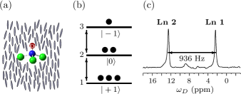
Figure 2: (a) A Deuterium spin-1 nucleus oriented in a liquid crystalline matrix. (b) Single-qutrit energy level diagram depicting the thermal equilibrium population distribution of the eigen vectors labeled as $\{1,2,3\}$ (corresponding to the qutrit eigenstates $|+1\rangle,|0\rangle,|-1\rangle$) respectively. (c) Deuterium NMR spectrum of the oriented chloroform-D molecule at 277 K. The spectral lines are labeled as Ln 1 and Ln 2. At 277 K the NMR spectrum shows an effective quadrupolar splitting of 936 Hz.

The qutrit density matrix can be written as

$$\rho=\frac{1}{3}I+\rho^{d}$$ (67)

In NMR experiments we have access only to the traceless deviation density matrix $\rho^{d}$, which can be expanded in in terms of the traceless $\Lambda$ matrices given in Eqn. (31)

$$\rho^{d}=\sum_{i=1}^{8}\langle\Lambda_{i}\rangle\Lambda_{i},$$ (68)

where $\langle\Lambda_{i}\rangle$ is the expectation value of $\Lambda_{i}$ in the state $\rho$ (which is the same as the expectation value of $\Lambda_{i}$ in the state $\rho^{d}$. $\rho^{d}$ in turn can be written in terms of these expectations values of $\Lambda$ matrices as follows

$$\rho^{d} = \frac{1}{2}\left(\begin{array}[]{ccc}\langle\Lambda_{3}\rangle+\frac{1}{\sqrt{3}}\langle\Lambda_{8}\rangle&\langle\Lambda_{1}\rangle-\iota\langle\Lambda_{2}\rangle&\langle\Lambda_{4}\rangle-\iota\langle\Lambda_{5}\rangle\\ \langle\Lambda_{1}\rangle+\iota\langle\Lambda_{2}\rangle&-\langle\Lambda_{3}\rangle+\frac{1}{\sqrt{3}}\langle\Lambda_{8}\rangle&\langle\Lambda_{6}\rangle-\iota\langle\Lambda_{7}\rangle\\ \langle\Lambda_{4}\rangle+\iota\langle\Lambda_{5}\rangle&\langle\Lambda_{6}\rangle+\iota\langle\Lambda_{7}\rangle&-\frac{2}{\sqrt{3}}\langle\Lambda_{8}\rangle\end{array}\right)$$ (72)

A single-qutrit density matrix has two single-quantum coherences (elements $\rho^{d}_{12}$ and $\rho^{d}_{23}$) that have a direct correspondence with the two NMR single-quantum transitions $1-2$ and $2-3$ respectively (Figure 2). From Eqn. (LABEL:qut-den), we have

$$\rho^{d}_{12} = \frac{1}{2}(\langle\Lambda_{1}\rangle-\iota\langle\Lambda_{2}\rangle),$$

$$\rho^{d}_{23} = \frac{1}{2}(\langle\Lambda_{6}\rangle-\iota\langle\Lambda_{7}\rangle)$$ (74)

and the expectation values in turn are determined by the real and imaginary parts of the intensity of the first line

(76)

Similarly, from the second spectral line, one obtains,

$$\langle\Lambda_{6}\rangle_{\rho} = \langle\Lambda_{6}\rangle_{\rho^{d}}=\mathfrak{Re}\{\mathbf{I}\textrm{({\bf Ln 2})}\}$$

$$\langle\Lambda_{7}\rangle_{\rho} = \langle\Lambda_{7}\rangle_{\rho^{d}}=-\mathfrak{Im}\{\mathbf{I}\textrm{({\bf Ln 2})}\}$$ (77)

III.2 Experimental scheme

A set of four NMR experiments can be used to evaluate the inequality described in (65). The experiments use transition-selective pulses of flip angle $\theta$ about the $j^{th}$ axis on transition $r-s$, along with non-unitary $z$-gradient pulses to kill unwanted coherences. The set of experiments are designed such that they project the directly inaccessible expectation values of the density matrix $\rho^{d}$ onto the single-quantum elements in the final state density matrix $\rho^{d}_{k}$ of the $k^{th}$ experiment. The protocol for finding the expectation values is designed to directly measure the required expectation values and avoid full quantum state tomography.

The experiments are delineated below:

• Experiment 1 : No operation

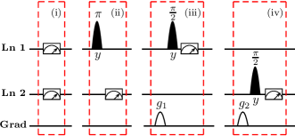
$\begin{array}[t]{rcl}\langle\Lambda_{1}\rangle_{\rho}&=&\mathfrak{Re}\{\mathbf{I}\textrm{({\bf Ln 1})}\}\\ \langle\Lambda_{6}\rangle_{\rho}&=&\mathfrak{Re}\{\mathbf{I}\textrm{({\bf Ln 2})}\}\end{array}$ • Experiment 2 : $(\pi_{y})^{1-2}$ $\begin{array}[t]{rcl}\langle\Lambda_{4}\rangle_{\rho}&=&\mathfrak{Re}\{\mathbf{I}\textrm{({\bf Ln 2})}\}\end{array}$ • Experiment 3 : Grad_z - $(\frac{\pi}{2}_{y})^{1-2}$ $\begin{array}[b]{rcl}\langle\Lambda_{3}\rangle_{\rho}&=&\mathfrak{Re}\{\mathbf{I}\textrm{({\bf Ln 1})}\}\end{array}$ • Experiment 4 : Grad_z - $(\frac{\pi}{2}_{y})^{2-3}$ $\begin{array}[t]{rcl}\langle\Lambda_{8}\rangle_{\rho}&=&\frac{1}{\sqrt{3}}\left[2\mathfrak{Im}\{\mathbf{I}\textrm{({\bf Ln 2})}\}\right.\left.+\langle\Lambda_{3}\rangle_{\rho}\par\right]\end{array}$ The expectation values obtained experimentally are substituted into left hand side of inequality (65), to test single-qutrit contextuality. The set of four experiments is shown diagrammatically in Figure 3 as four modules, numbered from (i)-(iv). All pulses are transition-selective ‘Gaussian’ shaped pulses of duration 400 $\mu s$, applied at the frequency offsets of Ln 1 and Ln 2 (Figure 2). Sine-shaped pulsed field gradients of strength $g_{i}$ along the $z$ axis are applied on the gradient channel (labeled ‘Grad’). The meter symbol in each experimental module denotes a measurement of the corresponding line intensity. Figure 3: NMR pulse sequence modules for single-qutrit contextuality measurements. Block (i) yields the expectation values $\langle\Lambda_{2}\rangle$ and $\langle\Lambda_{6}\rangle$, while (ii), (iii), (iv) yield the expectation values $\langle\Lambda_{4}\rangle$, $\langle\Lambda_{3}\rangle$ and $\langle\Lambda_{8}\rangle$ respectively. ‘Ln 1’ and ‘Ln 2’ correspond to the two single-quantum qutrit transitions and ‘Grad’ denotes the gradient channel. Pulse flip angles are shown at the top and the axes of rotation at the bottom of each pulse symbol .

III.3 Testing contextuality

The experimental tests of contextuality are performed on four different states at different time points. The results are shown in Figure 4 where the left hand side of the non-contextuality inequality given in (65) is plotted as a function of time.

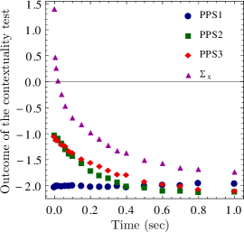
Figure 4: Plot showing the left hand side of inequality given in (65) for four different initial states at different time points. The blue circles correspond to the state ‘PPS1’, the green square markers markers represent the state ‘PPS2’, the red diamonds represent ‘PPS3’ and the purple triangles correspond to the state $\Sigma_{x}$.

We describe below the four states that we have used and their preparation schemes.

III.3.1 PPS1

The pseudopure state PPSI corresponding to the pure state $|+1\rangle$ is prepared by the sequence: $\left(\frac{\pi}{2}\right)_{y}^{(2-3)}$-Grad_z applied on the thermal equilibrium state of the single qutrit. The deviation density operator corresponding to this state is given by

$$\rho^{d}_{\rm PPS1}=\frac{1}{6}\left(\begin{array}[]{ccc}2&0&0\\ 0&-1&0\\ 0&0&-1\end{array}\right)$$ (86)

The left hand side of the contextuality inequality given in (65) has the value $-2$ for this state. Therefore, the state is contextual. The time evolution shown in Figure 4 reveals that the state moves towards the thermal equilibrium state, while remaining contextual at all times.

III.3.2 PPS2

The pseudopure state PPS2 corresponding to the pure state $|0\rangle$ is prepared by the sequence: $\left(\frac{\pi}{2}\right)_{y}^{(2-3)}$-Grad_z, $(\pi)_{y}^{(1-2)}$ and the corresponding deviation density operator is given by

$$\rho^{d}_{\rm PPS2}=\frac{1}{6}\left(\begin{array}[]{ccc}1&0&0\\ 0&-2&0\\ 0&0&1\end{array}\right)$$ (90)

The left hand side of inequality given in (65) has the value $-1$ for this state, showing that the PPS2 state is contextual. As this state evolves, it tends towards thermal equilibrium, which is reflected in the green square markers curve in Figure 4.

III.3.3 PPS3

The pseudopure state PPS3 corresponding to the pure state $|-1\rangle$ is prepared by the sequence: $\left(\frac{\pi}{2}\right)_{y}^{(1-2)}$-Grad_z with the corresponding deviation density operator given by

$$\rho^{d}_{\rm PPS3}=\frac{1}{6}\left(\begin{array}[]{ccc}1&0&0\\ 0&1&0\\ 0&0&-2\end{array}\right)$$ (94)

Inequality given in (65) has the value $-1$ for this state showing that this state is contextual. The time evolution takes this state towards thermal equilibrium as in the previous cases, while keeping the state contextual at all times.

III.3.4 Off-Diagonal Example

We generate a deviation density operator $\Sigma_{x}$ which does not contain any diagonal elements, by a non-selective $\left(\frac{\pi}{2}\right)_{y}$ pulse on the thermal equilibrium state.

$$\Sigma_{x}=\frac{1}{3\sqrt{2}}\left(\begin{array}[]{ccc}0&1&0\\ 1&0&1\\ 0&1&0\end{array}\right)$$ (98)

The contextuality value for this state is $+1.49$ and thus this state is non-contextual, corresponding to the set of vectors in Eqn. (61). This state approaches thermal equilibrium, as seen from Figure 4, and becomes contextual as it evolves.

III.4 Single-shot test for diagonal states

The contextuality test for all the diagonal states of a single qutrit can be performed in a single-shot measurement. If a state is prepared in a diagonal form, $\langle\Lambda_{1}\rangle=\langle\Lambda_{4}\rangle=\langle\Lambda_{6}\rangle=0$. Therefore for testing contextuality, one needs to find only the non-vanishing expectation values $\langle\Lambda_{3}\rangle$ and $\langle\Lambda_{8}\rangle$. The contextuality inequality in (65) reduces to

$$\langle-3\Lambda_{3}-\sqrt{3}\Lambda_{8}\rangle\geq 0$$ (99)

for this class of states. Consider an NMR experimental test consisting of sequential implementation of two unitary operators $\Lambda_{6}(\frac{\pi}{4})$ and $\Lambda_{2}(\frac{\pi}{4})$ on the diagonal state $\rho_{\rm diag}$

$$\rho_{\rm final}=e^{\iota\frac{\pi}{4}\Lambda_{2}}e^{\iota\frac{\pi}{4}\Lambda_{6}}\rho_{\rm diag}e^{-\iota\frac{\pi}{4}\Lambda_{6}}e^{-\iota\frac{\pi}{4}\Lambda_{2}}$$ (100)

The line intensity I$(\mathbf{Ln1})$ in the NMR spectrum of state $\rho_{\rm final}$ is given by:

$$\mathfrak{Re}\{\mathbf{I}(\mathbf{Ln1})\}=\frac{1}{4}(-3\langle\Lambda_{3}\rangle_{\rho_{\rm diag}}-\sqrt{3}\langle\Lambda_{8}\rangle_{\rho_{\rm diag}})$$ (101)

Comparing (99) and (101), we readily obtain a simple non-contextuality inequality for the diagonal state $\rho_{\rm diag}$

$$\mathfrak{Re}\{\textbf{I}\mathbf{(Ln1)}\}_{\rm final}\geq 0$$ (102)

The violation of the above inequality is a test for single-qutrit contextuality, which can be carried out in a single measurement.

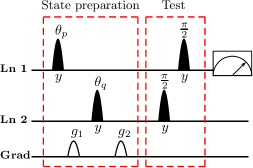
Figure 5: NMR pulse sequence for the creation of an arbitrary single-qutrit diagonal state, followed by a single-shot contextuality test for diagonal states. ‘Ln 1’ and ‘Ln 2’ correspond to the two single-quantum qutrit transitions and ‘$Grad$’ denotes the gradient channel. Pulse flip angles are shown at the top, and the axes of rotation at the bottom, of each pulse symbol.

Various single qutrit diagonal states are obtained from the thermal equilibrium density operator using the pulse sequence shown in Fig. 5. The set of deviation density matrices $\rho^{d}_{\rm diag}$ corresponding to the resulting diagonal states are given by

$$\rho^{d}_{\rm diag}=\left(\begin{array}[]{ccc}p&0&0\\ 0&q&0\\ 0&0&r\end{array}\right)$$ (106)

where $p=\cos^{2}{\frac{\theta_{p}}{2}}$, $q=\cos^{2}{\frac{\theta_{q}}{2}}\sin^{2}{\frac{\theta_{p}}{2}}-\sin^{2}{\frac{\theta_{q}}{2}}$ and $r=-(p+q)$. Angles $\theta_{p}$ and $\theta_{q}$ are chosen in the range $[0,\pi]$, giving rise to arbitrary diagonal single-qutrit states. State preparation is followed by the single-shot contextuality test. The parameters used for diagonal state preparation, as well as the theoretically expected and experimentally obtained values for the line intensity $\mathfrak{Re}\{\textbf{I}\mathbf{(Ln1)}\}_{\rm final}$ in (102) are shown in Table 1.

Table 1: Parameter values of the prepared single-qutrit diagonal states, values of $\theta_{p}$, $\theta_{q}$ (in degrees). The theoretically expected $\textbf{I}_{\rm Th}$ and experimentally measured $\textbf{I}_{\rm Exp}$ line intensity after the single-shot contextuality test are also shown.

No.	$~{}~{}\theta_{p}~{}$	$~{}~{}~{}\theta_{q}~{}$	p	q	r	$\textbf{I}_{\rm Th}$	$\textbf{I}_{\rm Exp}$
1	$0.0$	$0.0$	$0.33$	$0.00$	$-0.33$	$-2.00$	$-2.00$
2	$0.0$	$90.0$	$0.33$	$-0.17$	$-0.17$	$-2.00$	$-1.97$
3	$135.9$	$78.4$	$0.14$	$0.12$	$-0.26$	$-0.85$	$-0.83$
4	$140.7$	$81.6$	$0.11$	$0.08$	$-0.19$	$-0.68$	$-0.68$
5	$126.2$	$76.7$	$0.20$	$0.11$	$-0.31$	$-1.23$	$-1.13$

IV Concluding Remarks

Contextuality is an inherent property of quantum systems and has garnered much recent attention as a computational resource. A single qutrit is the simplest indivisible quantum system that can be used to demonstrate quantum contextuality. In this work, we perform an experimental NMR test to reveal single-qutrit contextuality, using a set of four measurements. The previously developed contextuality inequality based on nine observables was reformulated in terms of traceless observables that can be measured by NMR. The protocol was successfully implemented on a single-qutrit NMR quantum information processor to reveal the contextual properties of different quantum states. A single-shot contextuality test was also devised for the diagonal states of a qutrit. An experimental test of contextuality in a single qutrit is an important step towards understanding its strange quantum properties.