Consensus and Formation Control on $SE(3)$ for Switching Topologies

Abstract

This paper addresses the consensus problem and the formation problem on $SE(3)$ in multi-agent systems with directed and switching interconnection topologies. Several control laws are introduced for the consensus problem. By a simple transformation, it is shown that the proposed control laws can be used for the formation problem. The design is first conducted on the kinematic level, where the velocities are the control laws. Then, for rigid bodies in space, the design is conducted on the dynamic level, where the torques and the forces are the control laws. On the kinematic level, first two control laws are introduced that explicitly use Euclidean transformations, then separate control laws are defined for the rotations and the translations. In the special case of purely rotational motion, the consensus problem is referred to as consensus on $SO(3)$ or attitude synchronization. In this problem, for a broad class of local representations or parameterizations of $SO(3)$, including the Axis-Angle Representation, the Rodrigues Parameters and the Modified Rodrigues Parameters, two types of control laws are presented that look structurally the same for any choice of local representation. For these two control laws we provide conditions on the initial rotations and the connectivity of the graph such that the system reaches consensus on $SO(3)$. Among the contributions of this paper, there are conditions for when exponential rate of convergence occur. A theorem is provided showing that for any choice of local representation for the rotations, there is a change of coordinates such that the transformed system has a well known structure.

, ,

1 Introduction

This work addresses the problem of continuous time consensus and formation control on $SE(3)$ for switching interconnection topologies. We start by designing control laws on a kinematic level, where the velocities are control signals and then continue to design control laws on the dynamic level for rigid bodies in space, where the forces and the torques are the control laws.

The main focus in this paper is on the kinematic control laws. This approach is not justified from a physical perspective. Nevertheless, there are reasons why this path is still reasonable to take. Firstly, dynamics are often platform dependent, and especially in the robotics community it is desired to specify control laws on the kinematic level. Secondly, a deeper understanding of how the geometry of $SE(3)$ (and in particular $SO(3)$) affects the control design can be acquired by designing the control laws on a kinematic level, since we are then working directly in the tangent space of $SE(3)$ or $SO(3)$.

On $SE(3)$, consensus control is a special case of formation control, but actually formation control can be seen as a special case of consensus control, a fact that will be used in this paper. The approach is to develop consensus control laws, which after a simple transformation can be used as formation control laws. By taking this approach we can use existing theory for consensus in order to provide convergence results for the formation problem.

The consensus control problem on $SO(3)$ comprises a subset of the consensus control problem on $SE(3)$, but it is, from many perspectives, the most challenging part of the control design. Hence, most emphasis will be taken towards this problem. Whereas the translations are elements of $\mathbb{R}^{3}$, the rotations are elements of the compact manifold $SO(3)$, the group of orthogonal matrices in $\mathbb{R}^{3\times 3}$ with determinant equal to $1$.

There is a wide range of applications for the proposed control laws, e.g., satellites or spacecraft that shall reach a certain formation, multiple robotic arms that shall hold a rigid object or cameras that shall look in some desired directions (or the same direction in case of consensus). For rigid bodies in space, i.e., spacecraft or satellites, there has recently been an extensive research on the consensus on $SO(3)$ problem [1, 2, 3, 4, 5]. In that problem, the goal is to design a control torque such that the rotations of the rigid bodies become synchronized or reach consensus. There are also adjacent problems, such as the problem where a group of spacecraft shall follow a leader while synchronizing the rotations between each other [6, 7]. In the recent work by D. Lee et al. [8], a dynamic level control scheme is presented for spacecraft formation flying with collision avoidance.

In this work we propose six kinematic control laws. The first two are constructed as elements of $se(3)$; they are linear functions of the transformations or the relative transformations of neighboring agents. The third and fourth are defined for the rotations only. They are constructed for the tangent space of $SO(3)$ using the angular velocity. Finally, the fifth and the sixth control laws are defined for the translations only. They are constructed in the tangent space of $\mathbb{R}^{3}$. All the control laws lead to consensus (or equivalently formation) under different assumptions on the graphs, the initial conditions and measurable entities.

The results for consensus on $SO(3)$ expands on the publications [9, 10, 11], by considering a larger class of local representations. Moreover, Proposition 20 provides the result that for certain topologies and all the considered local representations, the rate of convergence is exponential. An interesting geometric insight is provided in Theorem 16 where it is shown that for any of the local representations considered, if the second rotation control law is used and the rotations initially are contained inside the injectivity region, there is a change of coordinates so that the system has a well known-structure.

Towards the end of this paper we also consider the second order dynamics and torque control laws for rigid bodies in space. We use methods similar to backstepping in order to generalize the kinematic control laws to this scenario. This generalization is only performed for the case of time-invariant topologies.

The paper proceeds as follows. In Section 2, preliminary concepts are defined such as Euclidean transformations, rotations, translations, network topologies and switching signal functions. The concept of local representations for the rotations is also are introduced. In Section 3, the problem formulation is given. Section 4 introduces the six kinematic control laws, which are categorized into two groups. Convergence results for the first group of control laws are provided in Section 5, whereas the second group is treated in Section 6. In Section 7 – for the application of rigid bodies in space – we provide results for control laws on the dynamic level.

2 Preliminaries

2.1 Euclidean transformations, rotations, and translations

We consider a system of $n$ agents with states in $SE(3)$, the group of Euclidean transformations. This means that each agent $i$ has a matrix

$$G_{i}(t)=\begin{bmatrix}R_{i}(t)&T_{i}(t)\\ 0&1\end{bmatrix}\in SE(3)$$

at each time $t\geq t_{0}$. The matrix $R_{i}(t)$ is an element of $SO(3)$, the matrix group which is defined by

$$SO(3)=\{R\in\mathbb{R}^{3\times 3}:R^{T}R=I,\text{det}(R)=1\}.$$

The vector $T_{i}(t)$ is an element in $\mathbb{R}^{3}$.

Each agent has a corresponding rigid body. We denote the world coordinate frame by $\mathcal{F}_{W}$ and the instantaneous body coordinate frame of the rigid body of each agent $i$ by $\mathcal{F}_{i}$. Let $R_{i}(t)\in SO(3)$ be the rotation of $\mathcal{F}_{i}$ in the world frame $\mathcal{F}_{W}$ at time $t$ and let $R_{ij}(t)\in SO(3)$ be the rotation of $\mathcal{F}_{j}$ in the frame $\mathcal{F}_{i}$, i.e.,

$$R_{ij}(t)=R_{i}^{T}(t)R_{j}(t).$$

We refer to $R_{i}(t)$ as absolute rotation and $R_{ij}(t)$ as relative rotation.

The vector $T_{i}(t)$ is the position of agent $i$ in $\mathcal{F}_{W}$ at time $t$. The relative positions between agent $i$ and agent $j$ in the frame $\mathcal{F}_{i}$ at time $t$ is

$$T_{ij}(t)=R_{i}^{T}(t)(T_{j}(t)-T_{i}(t)),$$

which in general is different from $T_{j}(t)-T_{i}(t)$, the relative positions between agent $i$ and agent $j$ in the world frame. In the same way as for the rotations, we refer to $T_{i}(t)$ as absolute translation and $T_{ij}(t)$ as relative translation.

The relative Euclidean transformation

$$G_{ij}(t)=G_{i}^{-1}(t)G_{j}(t)$$

$$=\begin{bmatrix}R_{i}^{T}(t)R_{j}(t)&R_{i}^{T}(t)(T_{j}(t)-T_{i}(t))\\ 0&1\end{bmatrix}$$

contains both the relative rotation and the relative translation. From now on, in general we suppress the explicit time-dependence for the variables, i.e., $G_{i}$ should be interpreted as $G_{i}(t)$.

2.2 Local representations for the rotations

For a vector $p=[p_{1},p_{2},p_{3}]^{T}$ in $\mathbb{R}^{3}$ we define $\widehat{{p}}=p^{\wedge}$ by

$$\widehat{{p}}=p^{\wedge}=\begin{bmatrix}0&-p_{3}&p_{2}\\ p_{3}&0&-p_{1}\\ -p_{2}&p_{1}&0\end{bmatrix}.$$ (1)

We also define $(\cdot)^{\vee}$ as the inverse of $(\cdot)^{\wedge}$, i.e., $(p^{\wedge})^{\vee}=p$.

We consider local representations or parameterizations of $SO(3)$. Often we simply refer to them as representations or parameterizations. In this context, what is meant by a local representation is a diffeomorphism $f:B_{r}(I)\rightarrow B_{r^{\prime},3}(0)\subset\mathbb{R}^{3}$, where $B_{r}(I)$ is an open geodesic ball around the identity matrix in $SO(3)$ of radius $r$ less than or equal to $\pi$, and $B_{r^{\prime},3}(0)$ is an open ball around the point $0$ in $\mathbb{R}^{3}$ with radius $r^{\prime}$. $\bar{B}_{r}(I)$ and $\bar{B}_{r^{\prime},3}(0)$ are the closures of said balls. If we write $B_{r,3}$ or $B_{r}$, this is short hand notation for $B_{r,3}(0)$ or $B_{r}(I)$ respectively. The same goes for the closed balls. The local representations can be seen as coordinates in a chart covering an open ball around the identity matrix in $SO(3)$.

A set in $SO(3)$ is convex if any geodesic shortest path segment between any two points in the set is contained in the set. The set is strongly convex if there is a unique geodesic shortest path segment contained in the set [12]. If $r=\pi$, $B_{r}(I)$ comprises almost all of $SO(3)$ (in terms of measure), and $B_{r}(I)$ is convex if and only if $r\leq\pi/2$. The radius $r$ is referred to as the radius of injectivity. The parameterizations that we use have the following special structure

$$f(R)=g(\theta)u,$$ (2)

where $\theta$ is the geodesic distance between $I$ and $R$ on $SO(3)$, also referred to as the Riemannian distance, written as $d(I,R)$. The variable $u\in\mathbb{S}^{2}$ is the rotational axis of $R$, and $g:(-r,r)\rightarrow\mathbb{R}$ is an odd, analytic and strictly increasing function such that $f$ is a diffeomorphism. On $B_{\pi}(I)$ the vector $u$ and the positive variable $\theta$ are obtained as functions of $R$ in the following way

$$\theta=\cos^{-1}\bigg{(}\frac{\text{trace}(R)-1}{2}\bigg{)},\quad u=\frac{1}{2\sin(\theta)}\begin{bmatrix}r_{32}-r_{23}\\ r_{13}-r_{31}\\ r_{21}-r_{12}\end{bmatrix},$$

where $R=[r_{ij}]$. Let us denote $y_{i}=f(R_{i})$ and $y_{ij}=f(R_{ij}).$ It holds that ${y}_{ij}=-{y}_{ji},\text{ but in general }{y}_{j}-{y}_{i}\neq{y}_{ij}.$ For each representation, i.e., choice of $g$, $r\leq\pi$ is the largest radius such that $f$ is a diffeomorphism. The radius $r$ is the radius of injectivity and depends on the representation, but we suppress this explicit dependence and throughout this paper, $r$ corresponds to the representation at hand, i.e., the one we have chosen to consider at the moment. For the representation at hand we also define

$$r^{\prime}=\sup_{s\uparrow r}g(s).$$

Some common representations are:

• The Axis-Angle Representation, in which case $g(\theta)=\theta$ and $r=r^{\prime}=\pi$. This representation is almost global. The set $SO(3)\backslash B_{\pi}(I)$ has measure zero in $SO(3)$. The Axis-Angle Representation is obtained from the logarithmic map by

  $${{x}}_{i} =(\text{Log}(R_{i}))^{\vee},$$

  $${{x}}_{ij} =(\text{Log}(R_{i}^{T}R_{j}))^{\vee}.$$

  In the other direction, a rotation matrix $R_{i}$ is obtained via the exponential map by

  $$R_{i}(x_{i})=\text{exp}(\widehat{x}_{i}).$$

  The matrix $R_{ij}$ is obtained by

  $$R_{ij}(x_{i},x_{j})=\text{exp}(\widehat{x}_{i})^{T}\text{exp}(\widehat{x}_{j}).$$

  The function $\text{exp}_{R_{i}}$ is the exponential map at $R_{i}$. Using this notation, the function exp is short hand notation for $\text{exp}_{I}$.
  

• The Rodrigues Parameters, in which case $g(\theta)=\tan(\theta/2)$. The corresponding $r$ and $r^{\prime}$ are equal to $\pi$ and $\infty$ respectively.
  

• The Modified Rodrigues Parameters, in which case $g(\theta)=\tan(\theta/4)$, $r=\pi$ and $r^{\prime}=1$. This representation is obtained from the rotation matrices by a second order Cayley transform [13].
  

• The representation $(R-R^{T})^{\vee}$, in which case $g(\theta)=\sin(\theta)$, and the corresponding $r$ and $r^{\prime}$ are $\pi/2$ and $1$ respectively. This representation is popular because it is easy to express in terms of the rotation matrices. Unfortunately, since $r=\pi/2$, only $B_{\pi/2}(I)$ is covered.
  

• The Unit Quaternions, or rather parts of it. The unit quaternion $q_{i}$, expressed as a function of the Axis-Angle Representation $x_{i}=\theta_{i}u_{i}$ of $R_{i}\in B_{\pi}(I)$, is given by

  $$q(x_{i})=(\cos(\theta_{i}/2),\sin(\theta_{i}/2)u_{i})^{T}\in\mathbb{S}^{3}.$$

  This means that we can choose the last three elements of the unit quaternion vector as our representation, i.e., $\sin(\theta_{i}/2)u_{i}$, in which case $r=\pi$. The unit quaternion representation is popular since the mapping from $SO(3)$ to the quaternion sphere is a Lie group homomorphism.

Let ${x}_{i}(t)$ and ${x}_{ij}(t)$ denote the axis-angle representations of the rotations $R_{i}(t)$ and $R_{ij}(t)$, respectively. In the following, since we are only addressing representations of (subsets of) $B_{\pi}(I)$, we choose ${x}(t)=[{x}_{1}^{T}(t),{x}_{2}^{T}(t),\ldots,{x}_{n}^{T}(t)]^{T}\in(B_{\pi,3}(0))^{n}$ as the state of the system instead of $(R_{1}(t),\ldots,R_{n}(t))\in(B_{\pi}(I))^{n}.$ Note that since $\theta_{i}=\|x_{i}\|$, it holds that $g(\theta_{i})=g(\|x_{i}\|)$. The variables $y_{i}$ and $y_{ij}$ can be seen as functions of $x_{i}$ and $x_{i},x_{j}$ respectively, i.e.,

$$y_{i}(x_{i}) =(f\circ\text{exp})(\widehat{x}_{i}),$$

$$y_{ij}(x_{i},x_{j}) =(f\circ\text{exp})(\text{Log}(R_{i}^{T}(x_{i})R_{j}(x_{j}))).$$

Since $x_{i}$ and $x_{j}$ are elements of the vector $x$, we can write $y_{i}(x)$ and $y_{ij}(x)$. When we write $y_{i}(t)$ and $y_{ij}(t)$, this is equivalent to $y_{i}(x(t))$ and $y_{ij}(x(t))$ respectively. If we want to emphasize the dependence of the initial condition, instead of writing $x(t)$ (or $y(t)$) we write $x(t,t_{0},x_{0})$ (or $y(t,t_{0},y_{0}))$ where $x_{0}$ is the initial state and $t_{0}$ is the initial time.

2.3 Kinematics

We denote the instantaneous angular velocity of $\mathcal{F}_{i}$ by ${\omega}_{i}$. From now on, until Section 7, we assume that $\omega_{i}$ is the control variable for the rotation of agent $i$. The kinematics for $R_{i}$ is given by

$$\dot{R}_{i}=R_{i}\widehat{\omega}_{i},$$

where $R_{i}\widehat{\omega}_{i}$ is an element of the tangent space $T_{R_{i}}SO(3)$.

The kinematics is given by

$$\dot{{x}}_{i} =L_{{x}_{i}}{\omega}_{i},$$ (3)

where the Jacobian (or transition) matrix $L_{{x}_{i}}$ is given by

$$L_{{x}_{i}}=L_{\theta_{i}{u}_{i}}=I_{3}+\frac{\theta}{2}\widehat{{u}}_{i}+\bigg{(}1-\frac{\text{sinc}(\theta_{i})}{\text{sinc}^{2}(\frac{\theta_{i}}{2})}\bigg{)}\widehat{{u}}_{i}^{2}.$$ (4)

The proof is found in [14]. The function $\mathrm{sinc}(\beta)$ is defined so that $\beta\mspace{3.0mu}\mathrm{sinc}(\beta)=\sin(\beta)$ and $\mathrm{sinc}(0)=1$. It was shown in [15] that $L_{\theta{u}}$ is invertible for $\theta\in(-2\pi,2\pi)$. Note however that $\theta\in[0,\pi)$ here.

The linear velocity of agent $i$, expressed in $\mathcal{F}_{i}$, is denoted by $v_{i}$. Up until Section 7, we assume that $v_{i}$ is the control variable for the translation of agent $i$. The time derivative of $T_{i}(t)$ is given by

$$\dot{T}_{i}(t)=R_{i}(t)v_{i}.$$

Define

$$\xi_{i}=\begin{bmatrix}\widehat{\omega}_{i}&v_{i}\\ 0&0\end{bmatrix}.$$

It holds that

$$\dot{G}_{i}(t)=G_{i}(t)\xi_{i}.$$

2.4 Dynamics

The dynamics for agent $i$ is given by

$$\dot{G}_{i} =G_{i}\xi_{i}$$

$$\dot{\xi}_{i} =\begin{bmatrix}(J_{i}^{-1}(-\widehat{\omega}_{i}J_{i}\omega_{i}+\boldsymbol{\tau}_{i}))^{\wedge}&(\frac{\boldsymbol{f}_{i}}{m_{i}}-\widehat{\omega}_{i}v_{i})\\ 0&0\end{bmatrix},$$

where $J_{i}$ is the inertia matrix, $m_{i}$ is the mass, $\boldsymbol{\tau_{i}}$ is the control torque, and $\boldsymbol{f}_{i}$ is control force – the latter two are given as a bold symbols since we do not want to mix them up with other defined entities.

2.5 Connectivity

Definition 1.

A directed graph (or digraph) $\mathcal{G}=(\mathcal{V},\mathcal{E})$ consists of a set of nodes, $\mathcal{V}=\{1,...,n\}$ and a set of edges $\mathcal{E}\subset\mathcal{V}\times\mathcal{V}$.

Each node in the graph corresponds to a unique agent. We also define neighbor sets or neighborhoods. Let $\mathcal{N}_{i}\in\mathcal{V}$ comprise the neighbor set (sometimes referred to simply as neighbors) of agent $i$, where $j\in\mathcal{N}_{i}$ if and only if $(i,j)\in\mathcal{E}$. We assume that $i\in\mathcal{N}_{i}$ i.e., we restrict the collection of graphs to those for which $(i,i)\in\mathcal{E}$ for all $i\in\mathcal{V}$.

A directed path of $\mathcal{G}$ is an ordered sequence of distinct nodes in $\mathcal{V}$ such that any consecutive pair of nodes in the sequence corresponds to an edge in the graph. An agent $i$ is connected to an agent $j$ if there is a directed path starting in $i$ and ending in $j$.

Definition 2.

A digraph is strongly connected if each node $i$ is connected to all other nodes.

Definition 3.

A digraph is quasi-strongly connected if there exists a rooted spanning tree or a center, i.e., at least one node such that all other nodes are connected to it.

An adjacency matrix $\mathcal{A}=[a_{ij}]$ for a graph $\mathcal{G}=(\mathcal{V},\mathcal{E})$ is a matrix where $a_{ij}\geq 0$ for all $i,j$, and furthermore $a_{ij}>0$ if and only if $(i,j)\in\mathcal{E}$ for all $i,j$. Given our definition of graph, i.e., Definition 1, there are infinitely many adjacency matrices for a graph.

From Definition 1 we see that there are $2^{n^{2}}$ directed graphs with $n$ nodes, i.e., the power set of the edge set. Since we assume that $(i,i)$ is an edge in the graph for all $i$, there are $2^{n^{2}-n}$ graphs we consider. For $k\in\{1,\ldots,2^{n^{2}-n}\}$ we associate a corresponding unique graph $\mathcal{G}_{k}=(\mathcal{V},\mathcal{E}_{k})$ and a unique adjacency matrix ${A}_{k}$. The ${A}_{k}$ matrices are constructed in the following way. We construct a positive adjacency matrix ${A}^{\prime}=[a_{ij}]$ for the complete (fully connected) graph. For the matrix ${A}_{k}=[a_{ij}^{k}]$, it holds that $a_{ij}^{k}=a_{ij}$ if $(i,j)\in\mathcal{E}_{k}$, otherwise $a_{ij}^{k}=0$. Thus, if $(i,j)\in\mathcal{E}_{k}$, we can write $a_{ij}$ instead of $a_{ij}^{k}$.

Now, for each agent $i$ there are $2^{n-1}$ unique neighborhoods $\mathcal{N}_{i}^{l}$, where $l\in\{1,\ldots,2^{n-1}\}$. Given $k\in\{1,\ldots,2^{n^{2}-n}\}$, for agent $i$ there is a unique $l\in\{1,\ldots,2^{n-1}\}$ such that $\mathcal{N}_{i}^{l}$ is the neighborhood of agent $i$ in the graph $\mathcal{G}_{k}$. Also, if each agent $i$ has chosen an $l\in\{1,\ldots,2^{n-1}\}$ such that $\mathcal{N}_{i}^{l}$ is the neighborhood of agent $i$, then there is a unique $k\in\{1,\ldots,2^{n^{2}-n}\}$ such that $\mathcal{G}_{k}$ is the graph for the system.

We are now ready to address time-varying graphs. In order to do so, for each agent $i$, we introduce a switching signal function

$$\sigma^{i}:\mathbb{R}\rightarrow\{1,\ldots,2^{n-1}\},$$

which is piece-wise constant and right-continuous. Let $\{\tau^{i}_{k}\}$ be the monotonically strictly increasing sequence of times for which $\sigma^{i}$ is discontinuous. We assume that there is a positive lower bound $\tau_{D}$ between two consecutive switches, i.e.,

$$\sup_{k}(\tau^{i}_{k+1}-\tau^{i}_{k})>\tau_{D}\quad\text{ for all }i.$$

The time-varying neighborhood of agent $i$ is $\mathcal{N}^{\sigma^{i}(t)}_{i}$.

Given the set of switching signal functions $\sigma^{i}$ we can construct a piece-wise constant and right-continuous switching signal function for the graph of the multi-agent system. This switching signal function $\sigma$ has range $\{1,\ldots,2^{n^{2}-n}\}$ and switching times

$$\{\tau_{k}\}=\bigcup_{i}\{\tau_{l}^{i}\},$$

where $\{\tau_{k}\}$ is monotonically strictly increasing in $k$. Note that for $\sigma$ it is not necessarily true that there is a positive lower bound on the dwell time between two consecutive switches as is the case for $\sigma^{i}$.

Now, between any two switching times, $\sigma(t)$ is equal to the $k$ for which the graph $\mathcal{G}_{k}$ it holds that the neighborhood of each agent $i$ is equal to $\mathcal{N}_{i}^{\sigma^{i}(t)}$.

Definition 4.

The union graph of $\mathcal{G}_{\sigma(t)}$ during the time interval $[t_{1},t_{2})$ is defined by

$$\mathcal{G}([t_{1},t_{2}))=\textstyle\bigcup_{t\in[t_{1},t_{2})}\mathcal{G}_{\sigma(t)}=(\mathcal{V},\textstyle\bigcup\nolimits_{t\in[t_{1},t_{2})}\mathcal{E}_{\sigma(t)}),$$

where $t_{1}<t_{2}\leq+\infty$.

Definition 5.

The graph $\mathcal{G}_{\sigma(t)}$ is uniformly (quasi-) strongly connected if there is $T^{\sigma}>0$ such that the union graph $\mathcal{G}([t,t+T^{\sigma}))$ is (quasi-) strongly connected for all $t$.

The idea of using an individual switching signal $\sigma^{i}$ for each agent, is that each agent shall be able to choose independently which neighbors it decides to receive information from.

Instead of using the term communication graph for $\mathcal{G}_{\sigma(t)}$, we deliberately use the terms neighborhood graph, connectivity graph or interaction graph. Direct communication does not necessarily take place between the agents in practice. Instead, they can choose to just observe each other via cameras or other sensors, i.e., indirect communication.

3 Consensus and formation control

3.1 Consensus

We start this section by introducing the consensus problem on $SE(3)$. Consensus on $SE(3)$ means that, as time tends to infinity, the set of transformations $(G_{1}(t),G_{2}(t),\ldots,G_{n}(t))\in(SE(3))^{n}$ approaches the consensus set where all the transformations are equal. The problem is to construct a distributed control law for each agent $i$, where only information from the neighbors $\mathcal{N}_{i}$ is used in the control law, such that the system reaches consensus. This information could be the relative transformations to the neighbors or the absolute transformations of the neighbors. An other desired property is that the velocities $\xi_{i}$ tend to zero sufficiently fast so that the transformations converge to a static transformation.

When we say that the Euclidean transformations of the agents “approaches” the consensus set, we mean that the rotations

$$(R_{1}(t),R_{2}(t),\ldots,R_{n}(t))\in SO(3)^{n}$$

approach $\{(R_{1},\ldots,R_{n})\in(\bar{B}_{q}(I))^{n}:R_{1}=\ldots=R_{n}\}$ and the translations

$$T^{\text{tot}}=[T_{1}^{T}(t),T^{T}_{2}(t),\ldots,T^{T}_{n}(t)]^{T}\in\mathbb{R}^{3n}$$

approach the set where all the translations are equal. For the translations the convergence is defined in terms of the Euclidean metric. For the rotations, the convergence is defined in terms of the Riemannian metric on $SO(3)$. If the rotations are contained within the region of injectivity of a local parameterization, asymptotic stability in terms of the Riemannian metric on $SO(3)$ is equivalent to asymptotic stability using the Euclidean metric in the parameterization domain for $x$.

The consensus problem on $SE(3)$ might seem uninteresting in practice, since for rigid bodies in space it is not physically possible to reach consensus in the positions. There are two reasons for considering this problem anyway. Firstly, if we look at the consensus problem as two subproblems, consensus in the rotations and consensus in the positions, the former is still interesting in practice and has received a great deal of attention lately. Secondly and more importantly, the consensus control problem is equivalent to the formation control problem after a change of coordinates. Thus, all the control laws we develop for the consensus control problems can also be used for the formation control problem after a simple transformation. This will be elaborated more in Section 3.2.

The subproblem of reaching consensus in the rotations is referred to as the attitude synchronization problem or consensus on $SO(3)$. Then we shall find a feedback control law ${\omega}_{i}$ for each agent $i$ using the local representations of either absolute rotations or relative rotations so that the absolute rotations of all agents converge to the set where all the rotations are equal as time goes to infinity, i.e.,

$$\|R_{i}(t)-R_{j}(t)\|\rightarrow 0,\text{ for all }i,j,\text{ as }t\rightarrow\infty,$$ (5)

or equivalently,

$$\hskip 25.60747pt\|R_{ij}(t)-I\|\rightarrow 0,\text{ for all }i,j,\>\>\text{as }t\rightarrow\infty.$$

If $y\in(B_{r^{\prime},3}(0))^{n}$ it is true that

$$R_{i}=R_{j} \Longleftrightarrow x_{i}=x_{j}\Longleftrightarrow x_{ij}=0$$ (6)

$$\Longleftrightarrow y_{i}=y_{j}\hskip 1.45107pt\Longleftrightarrow y_{ij}=0\quad\text{ for all }i,j.$$

We define the consensus set $\mathcal{A}$ in $\mathbb{R}^{3n}$ as follows:

$$\mathcal{A}=\{z=[z_{1}^{T},z_{2}^{T},\ldots,z_{n}^{T}]^{T}\in\mathbb{R}^{3n}:z_{i}=z_{j}\in\mathbb{R}^{3},\forall i,j\}.$$

According to (6) and the fact that the map

$$R_{i}\mapsto x_{i}$$

is a diffeomorphism on $B_{\pi}(I)$, (5) can equivalently be written as $x(t)\rightarrow\mathcal{A}$ as $t\rightarrow\infty$. This means that the solution approaches $\mathcal{A}$. Thus, provided we can guarantee that $y(t)\in(B_{r^{\prime},3}(0))^{n}$ for all $t\geq t_{0}$, where $t_{0}$ is the initial time, consensus on $SE(3)$ for the multi-agent system is the following

$$(x(t),T^{\text{tot}}(t))\rightarrow\mathcal{A}\times\mathcal{A},\quad\text{ as }t\rightarrow\infty.$$

A stronger assumption on the convergence to $\mathcal{A}\times\mathcal{A}$ is global uniform asymptotic stability of $\mathcal{A}\times\mathcal{A}$ relative to a strongly forward-invariant set, see Definition 6 and Definition 7 below. The distance from a point $z$ in $\mathbb{R}^{p}$ to a set $\mathcal{D}$ in $\mathbb{R}^{p}$ is defined by

$$\|z\|_{\mathcal{D}}=\inf_{w\in\mathcal{D}}\|z-w\|.$$

For a time-invariant system, forward invariance or positive invariance of a set means that every solution to the system with initial condition in the set is forward complete and the solution at any time greater than the initial time is contained in the set. For switched systems we have the following type of invariance. The $f$-vectors used in the following two definitions are locally defined in that context.

Definition 6.

Consider dynamical systems of the following class. The dynamical equation is given by

$$\dot{z}=f_{\sigma(t)}(z),$$

where $z(t)\in\mathbb{R}^{p}$ for some positive integer $p$. The right-hand side is switching between a finite set $\mathcal{F}=\{f_{k}\}$ of time-invariant functions according to a switching signal function $\sigma$. The switching signal function $\sigma$ is well-behaved in the sense that there are only finitely many switches on any compact time interval.

A set $\mathcal{D}\subset\mathbb{R}^{p}$ is strongly forward-invariant if for any time $t_{0}$, any $z_{0}\in\mathcal{D}$ and any such well behaved switching signal function $\sigma$ switching between functions in $\mathcal{F}$, the solution $z(t,t_{0},z_{0})$ exists, is unique, forward complete and contained in $\mathcal{D}$ for all $t\geq t_{0}$.

Definition 7.

Consider the dynamical system

$$\dot{z}=f(t,z),$$

where $y(t)\in\mathbb{R}^{p}$ for some positive integer $p$. A set $\mathcal{D}_{1}\subset\mathbb{R}^{p}$ is globally uniformly asymptotically stable relative to the compact strongly forward-invariant set $\mathcal{D}_{2}$, if

1. $\mathcal{D}_{1}$ is uniformly stable relative to $\mathcal{D}_{2}$, i.e., for every $\epsilon>0$, there is a $\delta(\epsilon)>0$ such that

   $$(\|z_{0}\|_{\mathcal{D}_{1}}\leq\delta,\>z_{0}\in\mathcal{D}_{2})\Longrightarrow$$

   $$(\|z(t_{2},t_{1},z_{0})\|_{\mathcal{D}_{1}}\leq\epsilon\>\textnormal{ for all }t_{1},t_{2}\textnormal{ where }t_{2}\geq t_{1}),$$

2. $\mathcal{D}_{1}$ is globally uniformly attractive relative to $\mathcal{D}_{2}$, i.e., for every $\epsilon>0$, there is a $\tau(\epsilon)>0$ such that

   $$z_{0}\in\mathcal{D}_{2}\Longrightarrow$$

   $$(\|z(t_{2},t_{1},z_{0})\|_{\mathcal{D}_{1}}\leq\epsilon\>\textnormal{ for all }t_{1},t_{2},$$

   $$\textnormal{ such that }t_{2}\geq t_{1}+\tau(\epsilon)).$$

One can show that if $\mathcal{A}$ is globally uniformly asymptotically stable relative to the strongly forward invariant set $(\bar{B}_{q,3}(0))^{n}$ for $x(t)$ where $q<\pi$, then the set $\{(R_{1},\ldots,R_{n})\in(\bar{B}_{q}(I))^{n}:R_{1}=\ldots=R_{n}\}$ is globally uniformly asymptotically stable relative to $(\bar{B}_{q}(I))^{n}$ (when the Riemannian metric is used). The notation of “strong forward invariance” is adopted from [16], where it is defined for hybrid systems.

3.2 Formation

The consensus problem has many applications in the cases where the motion is purely rotational, e.g., attitude synchronization for spacecraft or orientation alignment for cameras. However, as already mentioned, reaching consensus in the positions is obviously not physically possible for rigid bodies, but reaching a formation is.

The objective is to make the $G_{i}^{-1}(t)G_{j}(t)$ matrices converge to some desired $G^{*}_{ij}$ matrices. The $G^{*}_{ij}$ matrices are assumed to be transitively consistent in that

$$G^{*}_{ij}G^{*}_{jk}=G^{*}_{ik}\text{ for all }i,j,k.$$

A necessary and sufficient condition for transitive consistency [17, 18, 19] of the $G^{*}_{ij}$ is that there are $G^{*}_{i}$ such that

$$G^{*}_{ij}=G^{*-1}_{i}G^{*}_{j}\text{ for all }i,j.$$

In this light, we formulate the objective in the formation problem as follows. Given some desired constant Euclidean transformation matrices $G_{1}^{*},\ldots,G_{n}^{*}$, construct a control law for each agent $i$ such that

$$~{}\|G_{1}\left(t\right)-Q^{-1}(t)G_{1}^{*}\| \rightarrow 0,$$

$$~{}\|G_{2}\left(t\right)-Q^{-1}(t)G_{2}^{*}\| \rightarrow 0,$$

$$\>\vdots$$

$$~{}\|G_{n}\left(t\right)-Q^{-1}(t)G_{n}^{*}\| \rightarrow 0,$$

as $t\rightarrow\infty$, where $Q(t)$ is a Euclidean transformation. This implies that

$$\|G_{i}^{-1}\left(t\right)G_{j}\left(t\right)-G_{i}^{*-1}G_{j}^{*}\|\rightarrow 0\quad\text{ as }\quad t\rightarrow\infty.$$

Thus, in some (possibly time-varying) coordinate frame, the Euclidean transformation of agent $i$ converges to $G_{i}^{*}$ as time tends to infinity. Each matrix $G_{i}^{*}$ contains the rotation matrix $R_{i}^{*}$ and the translation $T_{i}^{*}$.

On a kinematic level the formation control problem is equivalent to the consensus problem. Let us define

$$\tilde{G}_{i}=G_{i}G_{i}^{*-1}\>\text{ and }\>\tilde{G}_{ij}=G_{i}^{*}G_{ij}G_{j}^{*-1},\quad\text{for all }i.$$

The kinematics for $\tilde{G}_{i}$ is given by

$$\dot{\tilde{G}}_{i}=G_{i}\xi_{i}G_{i}^{*-1}=\tilde{G}_{i}G_{i}^{*}\xi_{i}G_{i}^{*-1}=\tilde{G}_{i}\tilde{\xi}_{i},$$

where

$$\tilde{\xi}_{i} =G_{i}^{*}\xi_{i}G_{i}^{*-1}=\begin{bmatrix}\widehat{\tilde{\omega}}_{i}&\tilde{v}_{i}\\ 0&0\end{bmatrix}$$

$$=\begin{bmatrix}R_{i}^{*}\widehat{\omega}_{i}R_{i}^{*T}&-R_{i}^{*}\widehat{\omega}_{i}R_{i}^{*T}T_{i}^{*}+R_{i}^{*}v_{i}\\ 0&0\end{bmatrix}.$$

and

$${\xi}_{i} =G_{i}^{*-1}\tilde{\xi}_{i}G_{i}^{*}=\begin{bmatrix}\widehat{{\omega}}_{i}&{v}_{i}\\ 0&0\end{bmatrix}$$

$$=\begin{bmatrix}R_{i}^{*T}\widehat{\tilde{\omega}}_{i}R_{i}^{*}&R_{i}^{*T}(\widehat{\tilde{\omega}}_{i}T_{i}^{*}+\tilde{v}_{i})\\ 0&0\end{bmatrix}.$$

It easy to see that if the system reaches consensus in the $\tilde{{G}}_{i}$, it also reaches the desired formation. Thus, a consensus control law $\tilde{\xi}_{i}$ can be constructed for each agent and provided that each agent $i$ knows $G_{i}^{*}$, $\xi_{i}$ is obtained by $\xi_{i}=G_{i}^{*-1}\tilde{\xi}_{i}G_{i}^{*}$. In general, unless the design is limited to the $\omega_{i}$, the proposed control laws in the next section should be used for formation control of the $\tilde{\xi}_{i}$.

On the dynamic level we have that

$$\dot{\tilde{\omega}}_{i}=~{} R_{i}^{*}J_{i}^{-1}\left(-\left(R_{i}^{*T}\widehat{\tilde{\omega}}_{i}R_{i}^{*}\right)J_{i}R_{i}^{*T}\tilde{\omega}_{i}+\boldsymbol{\tau}_{i}\right),$$ (7)

$$\dot{\tilde{v}}_{i}=~{} R_{i}^{*}\left(\frac{\boldsymbol{f}_{i}}{m_{i}}-R_{i}^{*T}\widehat{\tilde{\omega}}_{i}\left(\widehat{\tilde{\omega}}_{i}T_{i}^{*}+\tilde{v}_{i}\right)\right)-\left(\dot{\tilde{\omega}}_{i}\right)^{\wedge}T_{i}^{*}.$$ (8)

For the control design on the dynamic level, the approach is to design a consensus control law for the $\tilde{\omega}_{i}$ and the $\tilde{v}_{i}$ and then track this desired kinematic control law using methods similar to backstepping. For control laws designed on the kinematic level, since the problems of consensus and formation are equivalent, we will only focus on the consensus problem. The consensus problem more tractable, since one can use existing theory for that problem. On the dynamic level we will also only consider the consensus problem – the formation control laws have a similar structure as the consensus control laws in this case.

4 Kinematic control laws

We use two approaches for the design of the $\xi_{i}$. The first approach is to treat $\xi_{i}$ as one control variable and design a feedback control law as an expression of the $G_{i}$, the second approach is to design $\omega_{i}$ and $v_{i}$ separately. Most emphasis will be on the second approach. The control laws in the first approach are referred to as the first control laws, whereas the control laws in the second approach are referred to as the second control laws.

The first control laws

We propose the following control laws based on absolute and relative transformations respectively.

$${\xi}_{i} =\sum_{j\in\mathcal{N}^{\sigma^{i}(t)}_{i}}a_{ij}\left(\left(G_{j}-G_{i})+(G_{i}^{-1}-G_{j}^{-1}\right)\right),$$ (9)

$${\xi}_{i} =\sum_{j\in\mathcal{N}^{\sigma^{i}(t)}_{i}}a_{ij}\left(G_{ij}-G_{ij}^{-1}\right).$$ (10)

The second control laws

In the first two control laws below, $y_{i}$ and $y_{ij}$ could be any of the local representations considered in Section 2.

$${\omega}_{i} =\sum_{j\in\mathcal{N}^{\sigma^{i}(t)}_{i}}a_{ij}({y}_{j}-{y}_{i}),\hskip 82.51299pt$$ (11)

$${\omega}_{i} =\sum_{j\in\mathcal{N}^{\sigma^{i}(t)}_{i}}a_{ij}{y}_{ij},$$ (12)

$${v}_{i} =\sum_{j\in\mathcal{N}^{\sigma^{i}(t)}_{i}}a_{ij}({T}_{j}-{T}_{i}),\hskip 82.51299pt$$ (13)

$${v}_{i} =\sum_{j\in\mathcal{N}^{\sigma^{i}(t)}_{i}}a_{ij}{T}_{ij}.$$ (14)

The structure of these second control laws and especially (11) and (13) are well known from the literature [20, 21]. In Section 6 we provide new results on the rate of convergence and regions of attractions for these control laws in this context. When the control laws are used for formation instead of consensus, the $\tilde{\xi}_{i}$ are designed instead of the $\xi_{i}$; the controllers are obtained through the relation

$$\tilde{\xi}_{i}=G_{i}^{*}\xi_{i}G_{i}^{*-1},$$

as given in Section 3.2. As an example, suppose all the $R_{i}$ rotations and all the desired $R_{i}^{*}$ rotations in the formation are equal to the identity matrix. Then the agents shall reach a desired formation in the positions only. All the agents construct $\tilde{v}_{i}$ according to (13) or (14) and solve for $v_{i}$ through the following relation

$$\begin{bmatrix}I&T_{i}^{*}\\ 0&1\end{bmatrix}^{-1}\begin{bmatrix}0&\tilde{v}_{i}\\ 0&0\end{bmatrix}\begin{bmatrix}I&T_{i}^{*}\\ 0&1\end{bmatrix}=\begin{bmatrix}0&\tilde{v}_{i}\\ 0&0\end{bmatrix}=\begin{bmatrix}0&v_{i}\\ 0&0\end{bmatrix}.$$

In this simple case $v_{i}=\tilde{v}_{i}$ and $\xi_{i}=\tilde{\xi}_{i}$. However, in general $\xi_{i}\neq\tilde{\xi}_{i}$.

The following two sections are devoted to the study of the control laws (9-14).

5 Results for the first control laws

Proposition 8.

Suppose the graph $\mathcal{G}_{\sigma(t)}$ is time-invariant and strongly connected. Suppose that each rotation is contained in $B_{\pi/2}(I)$, then if control law (9) is used, the set $(B_{\pi/2,3}(0))^{n}$ is strongly forward invariant for the dynamics of $x$ and

$$(x(t),T^{\text{tot}}(t))\rightarrow\mathcal{A}\times\mathcal{A}\quad\text{ as }t\rightarrow\infty.$$

Proposition 9.

Suppose the graph $\mathcal{G}_{\sigma(t)}$ is time-invariant and quasi-strongly connected. Suppose $q<\pi/4$, if all the rotations are contained in $\bar{B}_{q}(I)$, then if control law (10) is used, the set $(\bar{B}_{q,3}(0))^{n}$ is strongly forward invariant for the dynamics of $x$ and $\mathcal{A}\times\mathcal{A}$ is globally asymptotically stable relative to $(\bar{B}_{q,3}(0))^{n}\times\mathbb{R}^{3n}$.

Remark 10.

It can be shown that the results in propositions 8 and 9 are slightly more general. It is true that $(x(t),T^{\text{tot}}(t))$ converges to a fixed point in $\mathcal{A}\times\mathcal{A}$, i.e., not a limit cycle. This result is however not shown here.

In proposition 9, we only guarantee stability of a set instead of uniform stability of the set.

In the following two proofs, since the graph is time-invariant, we write $\mathcal{G}$ and $\mathcal{N}_{i}$ instead of $\mathcal{G}_{\sigma(t)}$ and $\mathcal{N}^{\sigma^{i}(t)}_{i}$ respectively. The graph Laplacian matrix $L(\mathcal{G},A)$ for the graph $\mathcal{G}$ with the adjacency matrix $A$, is

$$L(\mathcal{G},A)=D-A,$$

where

$$D=\text{diag}(d_{1},\ldots,d_{n})=\text{diag}\left(\sum_{j=1}^{n}a_{1j},\ldots,\sum_{j=1}^{n}a_{nj}\right).$$

Proof of Proposition 8: When the control law (9) is used, $\omega_{i}$ is given by the following expression

$${\omega}_{i}=\sum_{j\in\mathcal{N}_{i}}a_{ij}({y}_{j}-{y}_{i}),$$

where $y_{i}=\sin(\theta_{i})u_{i}$ for all $i$. This control law for $\omega_{i}$ is on the form (11) and we will later show that, provided the rotations are contained within the region of injectivity, which in this case is the ball around the identity with radius $\pi/2$, $x(t)$ approaches $\mathcal{A}$ asymptotically. Also, $(B_{\pi/2,3}(0))^{n}$ is forward invariant.

Given the initial states $x_{i}(t_{0})$, since there are finitely many agents, there is a positive $q<\pi/2$ such that $x(t_{0})\in(\bar{B}_{q,3}(0))^{n}$. Let $\mathcal{X}=(\bar{B}_{q,3}(0))^{n}\times\mathbb{R}^{3n}$ and define the two closed sets

$$\Gamma_{2} =\mathcal{A}\cap(\bar{B}_{q,3}(0))^{n}\times\mathbb{R}^{3n}$$

$$\Gamma_{1} =\mathcal{A}\cap(\bar{B}_{q,3}(0))^{n}\times\mathcal{A}.$$

We can choose the state space as $\mathcal{X}$ for $(x,T^{\text{tot}})$ since this set is forward invariant, see Proposition 11 in Section 6. We observe that $\Gamma_{1}\subset\Gamma_{2}\subset\mathcal{X}.$

On $\mathcal{X}$, the dynamics for $T_{i}$ is given by

$$\dot{T}_{i}=\sum_{j\in\mathcal{N}_{i}}a_{ij}\left(\left(R_{i}+R_{i}R_{j}^{T})\right)T_{j}-\left(R_{i}+I\right)T_{i}\right).$$

But on the set $\Gamma_{2}$ the dynamics for $T_{i}$ is given by

$$\dot{T}_{i}=\sum_{j\in\mathcal{N}_{i}}a_{ij}\left(\left(I+Q^{*}\right)\left(T_{j}-T_{i}\right)\right),\hskip 56.9055pt$$

where $Q^{*}\in\bar{B}_{q,3}(0)$ is some constant rotation matrix. On $\Gamma_{2}$, the dynamics for $T^{\text{tot}}$ is given by

$$\dot{T}^{\text{tot}}=-(L(\mathcal{G},A)\otimes(I+Q^{*}))T^{\text{tot}}.$$

By using the fact that the eigenvalues of $(I+Q^{*})$ have real parts strictly greater than zero, the fact that ($(B_{\pi/2,3}(0))^{n}$ is forward invariant), and the fact that $L(\mathcal{G},A)$ is the graph Laplacian matrix for a strongly connected graph, one can show that $\Gamma_{1}$ is exponentially stable relative to $\Gamma_{2}$. Now one can use Theorem 8 in [22] in order to show that $\Gamma_{1}$ is globally attractive relative to $\mathcal{X}.$ $\blacksquare$

Proof of Proposition 9: When the control law (10) is used, $\omega_{i}$ is given by the following expression

$${\omega}_{i}=\sum_{j\in\mathcal{N}_{i}}a_{ij}y_{ij},$$

where $y_{ij}=\sin(\theta_{ij})u_{ij}$ for all $i$. This control law for $\omega_{i}$ is on the form (12).

Let $\mathcal{X}=(\bar{B}_{q,3}(0))^{n}\times\mathbb{R}^{3n}$ and define the two closed sets

$$\Gamma_{2} =\mathcal{A}\cap(\bar{B}_{q,3}(0))^{n}\times\mathbb{R}^{3n}$$

$$\Gamma_{1} =\mathcal{A}\cap(\bar{B}_{q,3}(0))^{n}\times\mathcal{A}.$$

We observe that $\Gamma_{1}\subset\Gamma_{2}\subset\mathcal{X}.$ Proposition 14 in Section 6 in combination with the fact that the right-hand sides of the $\dot{T}_{i}$ are well-defined, guarantees that $\mathcal{X}$ is forward invariant and can serve as the state space for $(x,T^{\text{tot}})$. Also the set $\Gamma_{2}$ is globally uniformly asymptotically stable relative to $\mathcal{X}$.

On $\mathcal{X}$, the dynamics for $T_{i}$ is given by

$$\dot{T}_{i}=\sum_{j\in\mathcal{N}_{i}}a_{ij}\left(\left(T_{j}-T_{i}\right)-R_{i}R_{j}^{T}\left(T_{i}-T_{j}\right)\right),$$

but on the set $\Gamma_{2}$ the dynamics for $T_{i}$ is given by

$$\dot{T}_{i}=\sum_{j\in\mathcal{N}_{i}}a_{ij}\left(T_{j}-T_{i}\right).$$

The dynamics for $T^{\text{tot}}$ is given by

$$\dot{T}^{\text{tot}}=-(L(\mathcal{G},A)\otimes I)T^{\text{tot}},$$

where $L(\mathcal{G},A)$ is the graph Laplacian matrix for a quasi-strongly connected graph. It is well known that the consensus set is exponentially stable for this dynamics. Thus, the set $\Gamma_{1}$ is globally asymptotically stable relative to $\Gamma_{2}$. Now one can use Theorem 10 in [22] in order to show that $\Gamma_{1}$ is globally asymptotically stable relative to $\mathcal{X}.$ $\blacksquare$

5.1 Numerical experiments

In order to illustrate the relation between consensus and formation the following example is considered. For a system of five agents, in Figure 1 the convergence of the $\tilde{G}_{i}$ variables to consensus and the convergence of the $G_{i}$ variables to a desired formation is shown. The adjacency matrix was chosen to that of a quasi-strongly connected graph with entries equal to $0$, $1$ or $2$. The initial rotations are drawn from the uniform distribution over $B_{\pi/2}(I)$. Each initial translation vector is drawn from the uniform distribution over the unit box in $\mathbb{R}^{3}$. The initial $R_{i}(0)$ rotations and initial $T_{i}(0)$ translations are the building blocks of the $G_{i}(0)$ transformations. The desired $G^{*}_{i}$ are constructed in the same manner as the $G_{i}(0)$, after which the $\tilde{G}_{i}(0)$ transformations are constructed by $\tilde{G}_{i}(0)={G}_{i}(0)G_{i}^{*-1}$.

For the same initial conditions, the four upper plots in Figure 1 show the convergence when controller (9) is used, whereas the four lower plots in Figure 1 show the convergence when controller (10) is used. In each of these four subplots, the first plot is showing the difference $\|\tilde{G}_{i}(t)-\tilde{G}_{1}(t)\|_{\text{F}}$ for all $i$; the second plot is showing one of the elements of $\tilde{G}_{i}(t)$ for all $i$ as function of time, this element is the upper left one in the $\tilde{G}_{i}(t)$, i.e., it is an element of the rotation matrix; the third plot is showing the difference $\|{G}_{i}(t)-{G}_{1}(t)\|_{\text{F}}$ for all $i$ as function of time; the fourth plot is showing one of the elements of ${G}_{i}(t)$ as function of time for all $i$. This element is chosen as the upper left element in the ${G}_{i}(t)$.

The construction of the initial rotations in this example does not guarantee that initial rotations are contained in the regions specified in Proposition 8 and Proposition 9, yet the convergence is obtained for both control laws. For 1000 simulations with five agents and random quasi-strongly connected topologies, where the initial rotations are drawn from the uniform distribution over $SO(3)$ and the translations are drawn from the uniform distribution over the unit cube in $\mathbb{R}^{3}$, the $\tilde{G}_{i}(t)$ transformations converged to consensus 909 respective 910 times for the two different control laws, i.e., a success rate of over 90 $\%$. If the initial rotations in $\tilde{G}_{i}$ were drawn from the uniform distribution over $B_{\pi/2}(I)$ the transformations converged to consensus 1000 respective 1000 times for the two different control laws, i.e., a success rate of 100 $\%$.

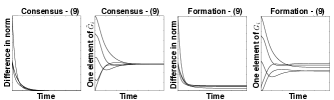
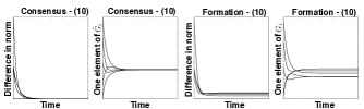
Figure 1: These plots illustrate the difference between reaching consensus in the $\tilde{G}_{i}$ variables and reaching a formation in the $G_{i}$ variables.

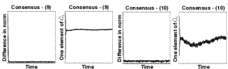
Figure 2: These plots show the convergence to consensus under discrete sampling, additive absolute noise, and switching between quasi-strongly connected graphs.

Furthermore, numerical experiments were conducted when there was additive absolute, noise and when the transformations were measured discretely the topologies were switching. The “noise” were random skew symmetric matrices, whose magnitudes were equal to $0.1$. Under these conditions the controllers (9) and (10) were tested in 100 simulations where the graphs were switching between quasi-strongly connected topologies and the initial rotations in $\tilde{G}_{i}$ were drawn from the uniform distribution over $B_{\pi/2}(I)$. The number of agents was 5. The matrices converged to consensus in every simulation for both controller (9) and controller (10). In the simulations the graphs switched with a frequency of $10$, which was the same as the sampling frequency; the consensus is shown for one simulation in Figure 2. The simulations show stronger results than those presented in Proposition 8 and Proposition 9.

The input is constant between sample points. Thus, we can solve the system exactly between those points (it becomes a linear time-invariant system). The solutions between the sampling points are not shown in the figure, instead there are straight lines connecting the solutions at the sample points.

In all simulations the “random” graphs were created by constructing adjacency matrices in the following way: First an adjacency matrix for a tree graph was created and then a binary matrix was created where each element in the matrix was drawn from the uniform distribution over $\{0,1\}$. The final adjacency was then chosen as the sum of the adjacency matrix for the tree graph and the binary matrix.

6 Results for the second control laws

6.1 Rotations

Here we address the controllers (11) and (12). We start with (11). The structure of controller (11) is well known from the consensus problem in a system of agents with single integrator dynamics and states in $\mathbb{R}^{m}$ [20]. The question is if this simple control law also works for rotations expressed in any of the local representations that we consider. The answer is yes. For all the convergence results provided in this section it is true that the state $x(t)$ converges to a fixed point, i.e., not a limit cycle.

Proposition 11.

Suppose $q<r$ and the graph $\mathcal{G}_{\sigma(t)}$ is uniformly strongly connected, then if controller (11) is used, $(\bar{B}_{q,3}(0))^{n}$ is strongly forward invariant, $0\in\mathbb{R}^{mn}$ is uniformly stable and $(\bar{B}_{q,3}(0))^{n}\cap\mathcal{A}$ is globally attractive relative to $(\bar{B}_{q,3}(0))^{n}$.

In order to prove Proposition 11, we use the following proposition.

Proposition 12.

Suppose controller (11) is used, $\mathcal{G}_{\sigma(t)}$ is uniformly strongly connected, and $q<r$.

Now, suppose there is a continuously differentiable function

$$V:\mathbb{R}^{3}\rightarrow\mathbb{R}$$

such that for any given $k\in\{1,\ldots 2^{n-1}\}$ and $\bar{x}=[\bar{x}_{1}^{T},\bar{x}_{2}^{T},\ldots,\bar{x}_{n}^{T}]^{T}\in(\bar{B}_{q,3}(0))^{n}$

1. if

   $$i\in\textnormal{arg}\max_{j\in\mathcal{N}^{k}_{i}}(V(\bar{x}_{j}))$$

   it holds that

   $$\langle\nabla V(\bar{x}_{i}),\sum_{j\in\mathcal{N}^{k}_{i}}a_{ij}({y}_{j}(\bar{x})-{y}_{i}(\bar{x}))\rangle\leq 0,$$ (15)

   where $y_{i}$ is the local representation.
   

2. and equality holds for (15) if and only if $\bar{x}_{i}=\bar{x}_{j}$ for all $j\in\mathcal{N}^{k}_{i}$,

then $(\bar{B}_{q,3}(0))^{n}$ is strongly forward invariant for the dynamics of $x$ and $(\bar{B}_{q,3}(0))^{n}\cap\mathcal{A}$ is globally attractive relative to $(\bar{B}_{q,3}(0))^{n}$.

The proof of Proposition 12 is omitted here but follows, up to small modifications, the procedure in the proof of Theorem 2.21. in [23]. The essential difference between the two is that besides the fact that in Theorem 2.21. in [23] more general right-hand sides of the system dynamics are considered, only one switching signal function is used for the system in that theorem, whereas in in this work we assume individual switching signal functions for the agents.

Proof of Proposition 11: We verify that (1) and (2) are satisfied in Proposition 12 by choosing $V(\bar{x}_{i})=\bar{x}_{i}^{T}\bar{x}_{i}$. Let $i\in\textnormal{arg}\max_{j\in\mathcal{N}^{k}_{i}}(V(\bar{x}_{j}))$. Then

$$\langle\nabla V(\bar{x}_{i}),\sum_{j\in\mathcal{N}^{k}_{i}}a_{ij}({y}_{j}(\bar{x})-{y}_{i}(\bar{x}))\rangle \leq$$

$$\sum_{j\in\mathcal{N}^{k}_{i}}(\|\bar{x}_{j}\|g(\|\bar{x}_{j}\|)-\|\bar{x}_{i}\|g(\|\bar{x}_{i}\|)) \leq 0,$$

where we have used the fact that $g$ is strictly increasing. The last inequality is strict if and only if $\bar{x}_{i}=\bar{x}_{j}$ for all $j\in\mathcal{N}^{k}_{i}$. $\blacksquare$

Remark 13.

Instead of using (11), one could use feedback linearization and construct the following control law for agent $i$,

$$\omega_{i}=L_{y_{i}}^{-1}\sum_{j\in\mathcal{N}^{\sigma^{i}(t)}_{i}}a_{ij}({y}_{j}-{y}_{i}),$$

where $L_{y_{i}}$ is the Jacobian matrix for the representation $y_{i}$. If this feedback linearization control law is used and the graph $\mathcal{G}_{\sigma(t)}$ is quasi-strongly connected, the consensus set, restricted to any closed ball $(\bar{B}_{q,3}(0))^{n}$ where $q<r$, is globally uniformly asymptotically stable relative to $(\bar{B}_{q,3})^{n}$. However, for many representations such as the Rodrigues Parameters, the Jacobian matrix $L_{y_{i}}$ is close to singular as $y_{i}$ is close to the boundary of $\bar{B}_{q,3}(0)$. Furthermore, the expression is nonlinear in the $y_{i}$. This might make this type of control law more sensitive to measurement errors than (11).

Now we continue with the study of (12) where only local representations of the relative rotations are available. Under stronger assumptions on the initial rotations of the agents at time $t_{0}$ and weaker assumptions on the graph $\mathcal{G}_{\sigma(t)}$, the following proposition ensures uniform asymptotic convergence to the consensus set.

Proposition 14.

Suppose $q<r/2$ and the controller (12) is used, then $(\bar{B}_{q,3}(0))^{n}$ is strongly forward invariant and $(\bar{B}_{q,3}(0))^{n}\cap\mathcal{A}$ is globally uniformly asymptotically stable relative to $(\bar{B}_{q,3}(0))^{n}$ if and only if $\mathcal{G}_{\sigma(t)}$ is uniformly quasi-strongly connected.

Remark 15.

In Proposition 14, since only information that is independent of $\mathcal{F}_{W}$ is used in (12), the assumption that the rotations initially are contained in $\bar{B}_{q}(I)$ can be relaxed. As long as there is a $Q\in SO(3)$ such that all the rotations are contained in $(\bar{B}_{q}(Q))^{n}$ initially, the rotations will reach consensus asymptotically and uniformly with respect to time.

In order to prove Proposition 14, we first provide a theorem, which gives some geometric insight. Then we provide a Proposition, which guarantees asymptotic stability of the consensus set.

Theorem 16.

Suppose that the control law (12) is used and $x\in(B_{q,3}(0))^{n}$, where $q<r/2$. Let $z_{i}=\tan(\theta_{i}/2)u_{i}$ and $z=[z_{1}^{T},\ldots,z_{n}^{T}]^{T}$. Then

$$\dot{z}_{1}= \sum_{j\in\mathcal{N}^{\sigma^{1}(t)}_{1}}a_{1j}h_{1j}(z_{1},z_{j})(z_{j}-z_{1}),$$

$$\vdots$$

$$\dot{z}_{n}= \sum_{j\in\mathcal{N}^{\sigma^{n}(t)}_{n}}a_{nj}h_{nj}(z_{n},z_{j})(z_{j}-z_{n}),$$

where $h_{ij}(z_{i},z_{j})\geq 0$ and $h_{ij}(z_{i},z_{j})>0$ if $z_{j}\neq z_{i}$.

Remark 17.

The $h_{ij}$ functions in Theorem 16 depends on the parameterization $y$.

A proof of Theorem 16 (up to small modifications due to the assumptions on the switching signal functions) can be found in [23]. It is based on the results in [12, 24]. Theorem 16 states that, after a change of coordinates to the Rodrigues Parameters, the system satisfies the well known convexity assumption that the right-hand side of each agent’s dynamics is inward-pointing [12] relative to the convex hull of its neighbors’ positions. There are many publications addressing this type of dynamics, e.g., [25, 26, 27].

Proposition 18.

Suppose control law (12) is used, $q<r/2$, and $(\bar{B}_{q,3}(0))^{n}$ is strongly forward invariant for the dynamics of $x$.

Suppose there is a continuously differentiable function

$$W:\mathbb{R}^{3}\times\mathbb{R}^{3}\rightarrow\mathbb{R}^{+},$$

such that for any given $k,l\in\{1,\ldots 2^{n-1}\}$ and $\bar{x}=[\bar{x}_{1}^{T},\bar{x}_{2}^{T},\ldots,\bar{x}_{n}^{T}]^{T}\in(\bar{B}_{q,3}(0))^{n}$,

1. if

   $$(i,j)\in\textnormal{arg}\max_{k^{\prime}\in\mathcal{N}^{k}_{i},l^{\prime}\in\mathcal{N}^{l}_{j}}(W(\bar{x}_{i},\bar{x}_{j}))$$

   it holds that

   $$\langle\nabla W(\bar{x}_{i},\bar{x}_{j}),[\left(\sum_{k^{\prime}\in\mathcal{N}^{k}_{i}}a_{ij}({y}_{k^{\prime}}(\bar{x})-{y}_{i}(\bar{x}))\right)^{T},$$

   $$\left(\sum_{l^{\prime}\in\mathcal{N}^{l}_{j}}a_{ij}({y}_{l^{\prime}}(\bar{x})-{y}_{j}(\bar{x}))\right)^{T}]\rangle \leq 0$$

2. and equality holds if and only if $\bar{x}_{i}=\bar{x}_{k^{\prime}}$ for all $k^{\prime}\in\mathcal{N}^{k}_{i}$ and $\bar{x}_{j}=\bar{x}_{l^{\prime}}$ for all $l^{\prime}\in\mathcal{N}^{l}_{j}$,

then $(\bar{B}_{q,3}(0))^{n}\cap\mathcal{A}$ is globally uniformly asymptotically stable relative to $(\bar{B}_{q,3}(0))^{n}$ if and only if $\mathcal{G}_{\sigma(t)}$ is uniformly quasi-strongly connected.

The proof of Proposition 18, is omitted here, but follows, up to small modifications, the procedure in the proof of Theorem 2.22. in [23].

Proof of Proposition 14: Let us define the functions

$$V(x_{i})= \>\>\>\>x_{i}^{T}x_{i}\text{ and }$$

$$W(x_{i},x_{j})= (z_{j}(x_{j})-z_{i}(x_{i}))^{T}(z_{j}(x_{j})-z_{i}(x_{i})),$$

Using Theorem 16 and the function $V$ together with Proposition 12, along the lines of the proof of Proposition 11, one can show that $(\bar{B}_{q,3}(0))^{n}$ is strongly forward invariant and if $\mathcal{G}_{\sigma(t)}$ is uniformly strongly connected, $(\bar{B}_{q,3}(0))^{n}\cap\mathcal{A}$ is globally attractive relative to $(\bar{B}_{q,3}(0))^{n}$.

Now, since $(\bar{B}_{q,3}(0))^{n}$ is strongly forward invariant, one can use Theorem  16 in order to show that $W$ satisfies the criteria in Proposition 18. The mapping

$$x_{i}\mapsto z_{i}$$

is a diffeomorphism on $(\bar{B}_{r,3}(0))^{n}$. The set $(\bar{B}_{q,3}(0))^{n}\cap\mathcal{A}$ is globally uniformly asymptotically stable relative to $(\bar{B}_{q,3}(0))^{n}$. $\blacksquare$

Remark 19.

We can generalize the results in Proposition 11 and Proposition 14. Up until now we have assumed that we first fix a representation $y_{i}$, $y_{ij}$ and then we use the control laws (11) and (12) for this representation. Instead, at each switching time $\tau_{k}^{i}$ we can allow the representation to switch also.

The following proposition addresses a special case when the the rate of convergence is exponential.

Proposition 20.

Suppose $\mathcal{G}_{\sigma(t)}$ fulfills the following. At each time $t$ and for each pair $(i,j)$, the edge $(i,j)\in\mathcal{E}_{\sigma(t)}$ or the edge $(j,i)\in\mathcal{E}_{\sigma(t)}$. Suppose controller (12) is used and $g(\theta_{i})\geq k\theta_{i}$ for some $k>0$. For $q<r/2$, the set $\{(R_{1},\ldots,R_{n})\in(\bar{B}_{q}(I))^{n}:R_{1}=\ldots=R_{n}\}$ is globally exponentially stable relative to $(\bar{B}_{q}(I))^{n}$ for the closed loop dynamics of $(R_{1},R_{2},\ldots,R_{n})$ with respect to the Riemannian metric on $SO(3)$.

Remark 21.

Using the results in [28] it can be obtained that for the Axis-Angle Representation the convergence is exponential also for general uniformly quasi-strongly connected graphs, i.e., not only the restricted class of graphs considered Proposition 20.

In Proposition 20 (1), since we have assumed that $g$ is analytic, the condition $g(\theta_{i})\geq k\theta_{i}$ can equivalently be formulated as $g(\theta_{i})=\mathcal{O}(\theta_{i})$ as $\theta_{i}\rightarrow 0$. All the local representations previously addressed fulfill this assumption, e.g., the Axis-Angle Representation, the Rodrigues Parameters and the Unit Quaternions.

Before we prove Proposition 20 we formulate the following lemma.

Lemma 22.

Suppose $x\in(\bar{B}_{q,3}(0))^{n}$ where $q<r/2$. If

$$(i,j)\in\textnormal{arg}\max_{(k,l)\in\mathcal{V}\times\mathcal{V}}\|x_{kl}\|,$$

then

$$x_{ij}^{T}y_{ik}\geq 0\quad\text{ for all }\quad k.$$

The proof of Lemma 22 follows more or less as a consequence of Theorem 16 and is omitted here.

Proof of Proposition 20: We already know from Proposition 14 that the set $(\bar{B}_{q,3}(0))^{n}$ is strongly forward invariant and $(\bar{B}_{q,3}(0))^{n}\cap\mathcal{A}$ is globally uniformly asymptotically stable relative to $(\bar{B}_{q,3}(0))^{n}$. What is left to prove is that for the special structure of the graph considered, the rate of convergence is exponential relative to $(B_{q}(I))^{n}$ when the Riemannian metric is used.

Let us define

$$\alpha=\min_{(k,l)\in\mathcal{V}\times\mathcal{V}}a_{kl},$$

and

$$V(x)=\max_{(k,l)\in\mathcal{V}\times\mathcal{V}}x_{kl}^{T}x_{kl}.$$

At time $t$ let $(i,j)$ be such that $V(x(t))=x^{T}_{ij}(t)x_{ij}(t)$.

$$x_{ij}^{T}\left(\omega_{j}-\omega_{i}\right)\leq-\alpha kV(x(t)),$$

where the last inequality is due to Lemma 22 and the assumption on the graph $\mathcal{G}_{\sigma(t)}$. Now one can show that

$$D^{+}V(x(t))\leq-\alpha kV(x(t)).$$

By using the Comparison Lemma, one can show that $V$ converges to zero with exponential rate of convergence. $\blacksquare$

6.2 Illustrative example

In order to illustrate the convergence of the rotations to the consensus set, an illustrative example is constructed where the representation $(R-R^{T})^{\vee}$ is chosen both for control law (11) and (12). The number of agents is $5$ and the graph the graphs were constructed in the same manner as in Section 5.1. The initial rotations are drawn from the uniform distribution over $B_{\pi/2}(I)$. The convergence to consensus is shown in Figure 3.

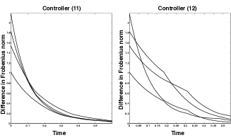
Figure 3: Convergence to consensus. For the same initial rotations, controller (11) and controller (12) are used. The left plot shows the errors (in terms of Frobenius norm) between the first rotation and the other rotations as a function of time when controller (11) is used; in the right plot the same type of errors is shown when controller (12) is used.

6.3 Translations

Here we address the controllers (13) and (14)

Controller (13), despite its appealing structure does in general not guarantee consensus in the translations. In order to see this, we consider the following example.

$$\dot{T}_{i}=\sum_{j\in\mathcal{N}^{\sigma^{i}(t)}_{i}}R_{i}^{T}(T_{j}-T_{i}).$$

Suppose

$$\begin{bmatrix}1&0&0\\ 0&1&0\\ 0&0&0\end{bmatrix}T_{i}(0)=T_{i}(0)\text{ and }$$

$$R_{i}(t)= \begin{bmatrix}-1&0&0\\ 0&-1&0\\ 0&0&1\end{bmatrix}\quad\text{ for all }i,t.$$

Then, for this particular choice of rotations and initial conditions for the $T_{i}$,

$$\dot{T}_{i}=\sum_{j\in\mathcal{N}^{\sigma^{i}(t)}_{i}}(T_{i}-T_{j}).$$

Thus,

$$\dot{T}^{\text{tot}}=(L(\mathcal{G}_{\sigma(t)},\mathcal{A})\otimes I)T^{\text{tot}},$$

which is unstable.

One partial result for controller (13) is the following one. By a change of coordinates one can prove that, if all the rotations of the agents are the same and constant and the translations are contained in the linear subspace spanned by the rotational axis, the translations converge asymptotically to consensus.

Controller (14) delivers a much stronger result.

Proposition 23.

Suppose controller (14) is used and the graph $\mathcal{G}_{\sigma(t)}$ is uniformly quasi-strongly connected. The set $\mathcal{A}$ is globally asymptotically stable stable.

The proof of the proposition is based on the fact that the closed loop dynamics is given by $\dot{T}^{\text{tot}}=-L(\mathcal{G}_{\sigma(t)},A)T^{\text{tot}}.$

7 Control on the dynamic level for rigid bodies in space

In this section we construct control laws on the dynamic level for the case of rigid bodies in space. The dynamical equations for agent $i$ are given by

$$\begin{cases}\dot{R}_{i}=R_{i}\widehat{\omega}_{i},\\ \dot{\omega}_{i}=J_{i}^{-1}\left(-\widehat{\omega}_{i}J_{i}\omega_{i}+\boldsymbol{\tau}_{i}\right),\\ \dot{T}_{i}=R_{i}v_{i},\\ \dot{v}_{i}=\frac{\boldsymbol{f}_{i}}{m_{i}}-\widehat{\omega}_{i}v_{i},\end{cases}$$ (16)

where $J_{i}$ is the inertia matrix and $\boldsymbol{\tau}_{i}$ is the control torque; $\omega_{i}$ is a state variable. In the formation problem the goal is to reach consensus in the $\tilde{(\cdot)}$-variables, and the dynamical equations for those variables are

$$\begin{cases}\dot{\tilde{R}}_{i}&=\tilde{R}_{i}\widehat{\tilde{\omega}}_{i},\\ \dot{\tilde{\omega}}_{i}&=R_{i}^{*}J_{i}^{-1}\left(-\left(R_{i}^{*T}\widehat{\tilde{\omega}}_{i}R_{i}^{*}\right)J_{i}R_{i}^{*T}\tilde{\omega}_{i}+\boldsymbol{\tau}_{i}\right),\\ \dot{\tilde{T}}_{i}&=\tilde{R}_{i}\tilde{v}_{i}\\ \dot{\tilde{v}}_{i}&=R_{i}^{*}\left(\frac{\boldsymbol{f}_{i}}{m_{i}}-R_{i}^{*T}\widehat{\tilde{\omega}}_{i}\left(\widehat{\tilde{\omega}}_{i}T_{i}^{*}+\tilde{v}_{i}\right)\right)-\left(\dot{\tilde{\omega}}_{i}\right)^{\wedge}T_{i}^{*}.\end{cases}$$ (17)

In this section, we strengthen the assumptions on $\mathcal{G}_{\sigma(t)}$ by assuming it is time-invariant. Thus, we denote the time-invariant (also referred to as constant or fixed) graph by $\mathcal{G}$. The reason for choosing time-invariant graphs is that we are now considering a second order system, and the methods we use here are based on backstepping. In order to show stability, we introduce auxiliary error variables, and in the case of a switching graph, these variables suffer from discontinuities. One way to avoid this problem is to replace the discontinuities with continuous in time transitions. This is however not something we do here.

7.1 Rotations

Only the consensus problem and the first set of equations, (16), will be considered here. When performing formation control, the presented control laws below, (18) and (19), are modified slightly. In both control laws, all the variables should be replaced by $\tilde{(\cdot)}$-variables, i.e., $x_{i}$ should be $\tilde{x}_{i}$ instead, $\tilde{\omega}_{i}$ should be ${\omega}_{i}$ instead and so on. The expression “$J_{i}$(” is replaced by “$J_{i}R_{i}^{T}$(”, and the expression “$\widehat{\omega}_{i}J_{i}\omega_{i}$” is replaced by “$\left(R_{i}^{*T}\widehat{\tilde{\omega}}_{i}R_{i}^{*}\right)J_{i}R_{i}^{*T}\tilde{\omega}_{i}$”.

Based on the two kinematic control laws (11) and (12), we now propose two torque control laws for each agent $i$, where the first one is based on absolute rotations and the second one is based on relative rotations. The control laws are

$$\boldsymbol{\tau}_{i} =J_{i}(-x_{i}+\sum_{j\in\mathcal{N}_{i}}a_{ij}(L_{x_{j}}\omega_{j}-L_{x_{i}}\omega_{i}-\bar{\omega}_{i}))+\widehat{\omega}_{i}J_{i}\omega_{i},$$ (18)

$$\boldsymbol{\tau}_{i} =J_{i}(-k_{i}\bar{\omega}_{i}^{\prime}+\sum_{j\in\mathcal{N}_{i}}a_{ij}L_{-y_{ij}}\omega_{ij})+\widehat{\omega}_{i}J_{i}\omega_{i}.$$ (19)

The parameter $k_{i}$ is a positive gain. The error variables $\bar{\omega}_{i}$ and $\bar{\omega}_{i}^{\prime}$ are by follows

$$\bar{\omega}_{i} =\omega_{i}-\sum_{j\in\mathcal{N}_{i}}a_{ij}(x_{j}-x_{i}),$$

$$\bar{\omega}_{i}^{\prime} =\omega_{i}-\sum_{j\in\mathcal{N}_{i}}a_{ij}y_{ij}.$$

The matrix $L_{y_{ij}}$ is the Jacobian matrix for $y_{ij}$, i.e.,

$$\dot{y}_{ij} =L_{-y_{ij}}\omega_{ij},$$

and

$$\omega_{ij}=R_{ij}\omega_{j}-\omega_{i}$$

is the relative angular velocity between agent $i$ and agent $j$. In the following, the notation $(x_{i},\bar{\omega}_{i}^{\prime})=[x_{i}^{T},\bar{\omega}_{i}^{\prime T}].$ We collect all the $x_{i}$ and $\bar{\omega}_{i}$ into $(x,\bar{\omega})\in(B_{\pi,3})^{n}\times(\mathbb{R}^{3})^{n}$ and all the $x_{i}$ and $\bar{\omega}_{i}^{\prime}$ into $(x,\bar{\omega}^{\prime})\in(B_{\pi,3})^{n}\times(\mathbb{R}^{3})^{n}$. Now, given $i\in\mathcal{V}$, the right-hand side for $(x_{i},\bar{\omega}_{i})^{T}$ when the torque control law (18) is used is

$$\dot{x}_{i} =L_{x_{i}}\sum_{j\in\mathcal{N}_{i}}a_{ij}(x_{j}-x_{i})+L_{x_{i}}\bar{\omega}_{i},$$

$$\dot{\bar{\omega}}_{i} =-x_{i}-\sum_{j\in\mathcal{N}_{i}}a_{ij}\bar{\omega}_{i},$$

whereas the closed loop system for $(x_{i},\bar{\omega}^{\prime}_{i})^{T}$ when the torque control law (19) is used, is

$$\dot{x}_{i} =L_{x_{i}}\sum_{j\in\mathcal{N}_{i}}a_{ij}y_{ij}+L_{x_{i}}\bar{\omega}_{i}^{\prime},\quad\quad\>\>\>$$

$$\dot{\bar{\omega}}_{i}^{\prime} =-k_{i}\bar{\omega}_{i}^{\prime}.$$

We note that in (18), each agent $i$ needs to know, not only the absolute rotations of its neighbors, but also the angular velocities of its neighbors. This requirement is fair, in the sense that in order to obtain the absolute rotations of the neighbors, communication is in general necessary. In this case the angular velocities can also be transmitted. In (19), we see that each agent $i$ needs to know the relative rotations, relative velocities to its neighbors and the angular velocity of itself. The assumption that agent $i$ knows its own angular velocity is quite strong the sense that this velocity is not to be regarded as relative information. However, in practice the angular velocity is possible to measure without the knowledge of the global frame $\mathcal{F}_{W}$. Thus, the angular velocity is local information.

Proposition 24.

Suppose $\mathcal{G}$ is strongly connected. If

$$\max_{i\in\mathcal{V}}\>x_{i}^{T}(t_{0})x_{i}(t_{0})+\bar{\omega}_{i}(t_{0})^{T}\bar{\omega}_{i}(t_{0})\leq q<\pi,$$

i.e., $(x_{i}(t_{0}),\bar{\omega}_{i}(t_{0}))^{T}\in\bar{B}_{q,6}$ for all $i$ and some $q<\pi$, then if controller (18) is used, $\bar{B}_{q,6}$ is invariant for $(x(t),\bar{\omega}(t))$ and $x(t)\rightarrow\mathcal{A}$ and $\omega_{i}(t)\rightarrow 0$ for all $i$ as $t\rightarrow\infty$.

Proof: In the multi-agent system at hand we have $n$ agents, where each agent $i$ has the state $(x_{i},\bar{\omega}_{i})^{T}$. We first show the invariance of the ball $\bar{B}_{q,6}$.

$$V((x_{i},\bar{\omega}_{i})^{T})=\frac{1}{2}\left(x_{i}^{T}x_{i}+\bar{\omega}_{i}^{T}\bar{\omega}_{i}\right).$$

We see that

$$\frac{d}{dt}V((x_{i},\bar{\omega}_{i})^{T})$$

$$= \sum_{j\in\mathcal{N}_{i}}a_{ij}(x_{i},\bar{\omega}_{i})(x_{j}-x_{i},-\bar{\omega}_{i})^{T}$$

$$= \sum_{j\in\mathcal{N}_{i}}a_{ij}((x_{i},\bar{\omega}_{i})(x_{j},0)^{T}-(x_{i},\bar{\omega}_{i})(x_{i},\bar{\omega}_{i})^{T})$$

$$\leq \sum_{j\in\mathcal{N}_{i}}a_{ij}x_{i}^{T}(x_{j}-x_{i}).$$

Thus,

$$D^{+}f_{V,6}((x(t),\bar{\omega}(t))^{T})\leq 0.$$

Now, by using the Comparison Lemma one can show the invariance.

In order to show the convergence, we define the following function

$$\bar{\gamma}(x,\bar{\omega})=\sum_{i=1}^{n}\xi_{i}(x_{i}^{T}x_{i}+\bar{\omega}_{i}^{T}\bar{\omega}_{i}),$$

where $\xi=(\xi_{1},\ldots,\xi_{n})^{T}$ is the positive vector chosen such that (the symmetrical part of) $\text{diag}(\xi)L(\mathcal{G},A)$ is positive semi-definite. We have that

$$\dot{\bar{\gamma}}=-{x}^{T}({L}^{\prime}\otimes{I}_{3}){x}-\sum_{i=1}^{n}\xi_{i}\sum_{j\in\mathcal{N}_{i}}a_{ij}\bar{\omega}_{i}^{T}\bar{\omega}_{i}.$$

By LaSalle’s theorem, $(x(t),\bar{\omega}(t))^{T}$ will converge to the largest invariant set contained in

$$\{(x,\bar{\omega})^{T}:\dot{\bar{\gamma}}((x,\bar{\omega})^{T})~{}=0\}$$

as the time goes to infinity. This largest invariant set is contained in the set $\{(x,\bar{\omega})^{T}:x\in\mathcal{A},\bar{\omega}=0\}$. $\blacksquare$

Remark 25.

In the proof of Proposition  24, if we look at the dynamics of $(x,\bar{\omega})$, we see that the largest invariant set contained in $\{(x,\bar{\omega})^{T}:\dot{\bar{\gamma}}((x,\bar{\omega})^{T})~{}=0\}$ is actually the point $0$. Hence, the system will reach consensus in the point $x=0$.

Now let us turn to control law (19).

Proposition 26.

Suppose $\mathcal{G}$ is quasi-strongly connected. For any positive $r_{1}$ and $r_{2}$ such that $r_{1}<r_{2}<r/2$ and $q>0$, there is a $k>0$ such that if $k_{i}\geq k$ and $(x_{i}(t_{0}),\bar{\omega}_{i}^{\prime}(t_{0}))^{T}\in\bar{B}_{r_{1},3}\times\bar{B}_{q,3}$ for all $i$, then if controller (19) is used it holds that $(x_{i}(t),\bar{\omega}_{i}^{\prime}(t))^{T}\in\bar{B}_{r_{2},3}\times\bar{B}_{q,3}$ for all $i,t\geq t_{0}$ and

$$(x(t),\bar{\omega}^{\prime}(t))^{T}\rightarrow(\bar{B}_{r_{2},3})^{n}\cap\mathcal{A}\times\{0\}\quad\text{ as }\quad t\rightarrow\infty.$$

Furthermore, $(\bar{B}_{r_{2},3})^{n}\cap\mathcal{A}\times\{0\}$ is globally asymptotically stable relative to the largest invariant set contained in $(\bar{B}_{r_{2},3})^{n}\times(\bar{B}_{q,3})^{n}$ for the dynamics of $(x(t),\bar{\omega}^{\prime}(t))^{T}$.

Proof of Proposition 26: Let us define

$$\mathcal{D}^{*}\subset\mathcal{D}=(\bar{B}_{r_{2},3})^{n}\times(\bar{B}_{q,3})^{n},$$

as the largest invariant set contained in $\mathcal{D}$. The set $\mathcal{D}^{*}$ is compact and implicitly a function of $k$ (or the $k_{i}$).

Now we show that for a proper choice of the constant $k$, it holds that

$$(\bar{B}_{r_{1},3})^{n}\times(\bar{B}_{q,3})^{n}\subset\mathcal{D}^{*}.$$

We assume without loss of generality that $t_{0}=0$, and note that

$$\|\bar{\omega}_{i}^{\prime}(t)\|=\|\bar{\omega}_{i}^{\prime}(0)\|\exp(-k_{i}t)\leq q\exp(-k_{i}t)\leq q\exp(-kt).$$

We choose

$$V(x_{i}(t))=x_{i}^{T}(t)x_{i}(t).$$

By using Lemma 22, it is possible to show that there exists an interval $[0,t_{1})$ on which it holds that

$$D^{+}(\max_{i}V(x(t)))\leq qr_{2}\exp(-kt).$$

By using the Comparison Principle, it follows that

$$\max_{i}V(x_{i}(t))\leq\max_{i}V(x_{i}(0))+qr_{2}\frac{(1-\exp(-kt))}{k}$$

on $[0,t_{1})$. Now if we choose $k\geq qr_{2}/(r_{2}-r_{1})$ we see that $\max_{i}V(x_{i}(t))\leq r_{2}$ for $t\geq 0$, and we can choose $t_{1}=\infty$.

In order to show the desired convergence we use Theorem 10 in [22], where $\mathcal{X}=\mathcal{D}^{*}$, $\Gamma_{2}=\mathcal{D}^{*}\cap((\bar{B}_{r_{2},3})^{n}\times\{0\})$ and $\Gamma_{1}=\mathcal{D}^{*}\cap(\mathcal{A}\times\{0\})$. $\blacksquare$

7.2 Translations

Also in this section only the consensus problem and the first set of equations, (16), are considered here. We introducing a generalized version of the control law (14). When the formation control problem is considered the all variables are replaced by $\tilde{(\cdot)}$-variables. Furthermore the expression “$m_{i}($” is replaced by “$m_{i}R_{i}^{*T}($”, and the expression “$\widehat{\omega}_{i}v_{i}$” is replaced by “$\widehat{\tilde{\omega}}_{i}(\widehat{\tilde{\omega}}_{i}T_{i}^{*}+\tilde{v}_{i}))+(\dot{\tilde{\omega}}_{i})^{\wedge}T_{i}^{*}$”.

The proposed consensus controller is

$$\boldsymbol{f}_{i}= m_{i}(-k_{i}\bar{v}_{i}+\sum_{j\in\mathcal{N}_{i}}a_{ij}R_{i}^{T}(R_{j}v_{j}-R_{i}v_{i})$$

$$-\sum_{j\in\mathcal{N}_{i}}a_{ij}\widehat{\omega}_{i}R_{i}^{T}(T_{j}-T_{i})+\widehat{\omega}_{i}v_{i}),$$

where

$$\bar{v}_{i}=v_{i}-\sum_{j\in\mathcal{N}_{i}}a_{ij}{T}_{ij}.\hskip 14.22636pt$$

The closed loop dynamics is

$$\hskip 28.45274pt\dot{T}_{i} =\sum_{j\in\mathcal{N}_{i}}a_{ij}(T_{j}-T_{i})+R_{i}(t)\bar{v}_{i}$$

$$\dot{\bar{v}}_{i} -k_{i}\bar{v}_{i}.$$

By treating the time as a variable $z$, we get the following system

$$\dot{z} =1$$

$$\hskip 28.45274pt\dot{T}_{i} =\sum_{j\in\mathcal{N}_{i}}a_{ij}(T_{j}-T_{i})+R_{i}(z)\bar{v}_{i}$$

$$\dot{\bar{v}}_{i} -k_{i}\bar{v}_{i}.$$

Let the state of the entire system be $(z,T^{\text{tot}},\bar{v}^{\text{tot}})$, where $v^{\text{tot}}=[\bar{v}_{1}^{T}(t),\bar{v}_{2}^{T}(t),\ldots,\bar{v}_{n}^{T}(t)]^{T}\in\mathbb{R}^{3n}$.

Proposition 27.

Suppose that $R_{i}(z)$ is well behaved, in the sense that the right-hand side of the dynamics for $(z,T^{\text{tot}},{v}^{\text{tot}})$ is locally Lipschitz, then the set $\mathbb{R}\times\mathcal{A}\times 0$ is globally asymptotically stable for the system.

Proof: Let the state space be $\mathcal{X}=\mathbb{R}\times\mathbb{R}^{3n}\times\mathbb{R}^{3n}$. We define the two closed subsets $\Gamma_{1}\subset\Gamma_{2}$ of $\mathcal{X}$ as follows

$$\Gamma_{1} =\mathbb{R}\times\mathcal{A}\times 0$$

$$\Gamma_{2} =\mathbb{R}\times\mathbb{R}^{3n}\times 0$$

It is easy to show that $\Gamma_{2}$ is globally asymptotically stable relative to $\mathcal{X}$ and $\Gamma_{1}$ is globally asymptotically stable relative to $\Gamma_{2}$. Now the desired result follows from Theorem 10 in [22]. $\blacksquare$

7.3 Illustrative examples

In Figure 4 the convergence to consensus is shown when controllers (18), (19) and (20) are used. In the simulations, five agents were considered and a random quasi-strongly connected graph was used. The convergence to consensus is shown for the rotations, left plots, and the translation, right plots, when controller (18) was used together with controller (20) and controller (19) was used together with controller (20). The left plots shows the Euclidean distance between $x_{i}(t)$ and $x_{1}(t)$ for $i=2,\ldots,5$, and the right plots show the Euclidean distance between $T_{i}$ and $T_{1}$ as a function of time for $i=2,\ldots,5$.

In controller (19) as well as controller (20) the $k_{i}$ were chosen to $3$ for all $i$. The adjacency matrix was chosen to that of a quasi-strongly connected graph with entries equal to $0$, $1$ or $2$. In controller (19) the representation $(R-R^{T})^{\vee}$ was used as the local representation for the $y_{ij}$.

Conclusions

This work has considered the consenus and formation problems on $SE(3)$ for multi-agent systems with switching interaction topologies. By a change of coordinates it was shown that the consensus problem can be seen as equivalent to the formation problem. Any control law designed for the consensus problem can, after change of coordinates, be used for the formation problem. New kinematic control laws have been presented as well as new convergence results. It has been shown that the same type of control laws can be used for many popular local representations of $SO(3)$ such as the Modified Rodrigues Parameters and the Axis-Angle Representation. It has been shown that some of the control laws guarantee almost global convergence. For non-switching topologies, the kinematic control laws have been extended to torque and force control laws for rigid bodies in space. The proposed control approaches have been justified by numerical simulations.

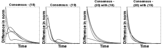
Figure 4: Convergence to consensus.

References

- [1] K. D. Listmann, C. A. Woolsey, and J. Adamy. Passivity-based coordination of multi-agent systems: a backstepping approach. In Proceedings of the European Control Conference 2009, pages 2450–2455. IEEE, 2009.
- [2] D. V. Dimarogonas, P. Tsiotras, and K. J. Kyriakopoulos. Laplacian cooperative attitude control of multiple rigid bodies. In Proceedings of the International Symposium on Intelligent Control, pages 3064–3069. IEEE, 2006.
- [3] A. Sarlette, R. Sepulchre, and N. E. Leonard. Autonomous rigid body attitude synchronization. Automatica, 45(2):572–577, 2009.
- [4] W. Ren. Distributed cooperative attitude synchronization and tracking for multiple rigid bodies. IEEE Transactions on Control Systems Technology, 18(2):383–392, 2010.
- [5] R. Tron, B. Afsari, and R. Vidal. Intrinsic consensus on so (3) with almost-global convergence. In Proceedings of the Conference on Decision and Control, CDC, pages 2052–2058. IEEE, 2012.
- [6] W. Kang and H-H. Yeh. Co-ordinated attitude control of multi-satellite systems. International Journal of robust and nonlinear control, 12(2-3):185–205, 2002.
- [7] D.V. Dimarogonas, P. Tsiotras, and K.J. Kyriakopoulos. Leader–follower cooperative attitude control of multiple rigid bodies. Systems & Control Letters, 58(6):429–435, 2009.
- [8] D. Lee, A.K. Sanyal, and E.A. Butcher. Asymptotic tracking control for spacecraft formation flying with decentralized collision avoidance. Journal of Guidance, Control, and Dynamics, 38(4):587–600, 2014.
- [9] J. Thunberg, E. Montijano, and X. Hu. Distributed attitude synchronization control. In 50th IEEE Conference on Decision and Control and European Control Conference, pages 1962–1967. IEEE, 2011.
- [10] W. Song J. Thunberg and X. Hu. Distributed attitude synchronization control of multi-agent systems with directed topologies. In 10th World Congress on Intelligent Control and Automation (WCICA), 2012, 2012.
- [11] J. Thunberg, W. Song, E. Montijano, Y. Hong, and X. Hu. Distributed attitude synchronization control of multi-agent systems with switching topologies. Automatica, 50(3):832–840, 2014.
- [12] B. Afsari. Riemannian l p center of mass: Existence, uniqueness, and convexity. Proceedings of the American Mathematical Society, 139(2):655–673, 2011.
- [13] P. Tsiotras, J.L. Junkins, and H. Schaub. Higher-order cayley transforms with applications to attitude representations. Journal of Guidance, Control, and Dynamics, 20(3):528–534, 1997.
- [14] J.L. Junkins and H. Schaub. Analytical mechanics of space systems. AIAA Education Series, 2003.
- [15] E. Malis, F. Chaumette, and S. Boudet. 2 1/2 D visual servoing. IEEE Transactions on Robotics and Automation, 15(2):238–250, 1999.
- [16] R. Goebel, R. G Sanfelice, and A. Teel. Hybrid Dynamical Systems: modeling, stability, and robustness. Princeton University Press, 2012.
- [17] R. Tron and R. Vidal. Distributed 3-d localization of camera sensor networks from 2-d image measurements. IEEE Transactions on Automatic Control, 59(12):3325–3340, 2014.
- [18] F. Bernard, J. Thunberg, P. Gemmar, F. Hertel, A. Husch, and J. Goncalves. A solution for multi-alignment by transformation synchronisation. In Conference on Computer Vision and Pattern Recognition. IEEE, 2015.
- [19] J. Thunberg, F. Bernard, and J Goncalves. On transitive consistency for linear invertible transformations between euclidean coordinate systems. arXiv preprint arXiv:1509.00728, 2015.
- [20] M. Mesbahi and M. Egerstedt. Graph theoretic methods in multiagent networks. Princeton University Press, 2010.
- [21] W. Ren and R. Beard. Distributed consensus in multi-vehicle cooperative control: theory and applications. Springer, 2007.
- [22] M. El-Hawwary and M. Maggiore. Reduction theorems for stability of closed sets with application to backstepping control design. Automatica, 49:214–222, 2013.
- [23] J. Thunberg, W. Song, Y. Hong, and X. Hu. Distributed attitude synchronization using backstepping and sliding mode control. Journal of Control Theory and Applications, 12(1):48–55, 2014.
- [24] J. Hartley, R. Trumpf and Y. Da. Rotation averaging and weak convexity. In Proceedings of the 19th International Symposium on Mathematical Theory of Networks and Systems (MTNS), pages 2435–2442, 2010.
- [25] L. Moreau. Stability of multiagent systems with time-dependent communication links. IEEE Transactions on Automatic Control, 50(2):169–182, 2005.
- [26] G. Shi and Y. Hong. Global target aggregation and state agreement of nonlinear multi-agent systems with switching topologies. Automatica, 45(5):1165–1175, 2009.
- [27] B. Francis Z. Lin and M. Maggiore. State agreement for continuous-time coupled nonlinear systems. SIAM Journal on Control and Optimization, 46(1):288–307, 2007.
- [28] S. Chen, L. Zhao, W. Zhang, and P. Shi. Consensus on compact Riemannian manifolds. Information Sciences, 268(C):220–230, June 2014.