Search for Gamma-ray Lines towards Galaxy Clusters with the Fermi-LAT

Abstract

We report on a search for monochromatic $\gamma$-ray features in the spectra of galaxy clusters observed by the Fermi Large Area Telescope. Galaxy clusters are the largest structures in the Universe that are bound by dark matter (DM), making them an important testing ground for possible self-interactions or decays of the DM particles. Monochromatic $\gamma$-ray lines provide a unique signature due to the absence of astrophysical backgrounds and are as such considered a smoking-gun signature for new physics. An unbinned joint likelihood analysis of the sixteen most promising clusters using five years of data at energies between 10 and 400 GeV revealed no significant features. For the case of self-annihilation, we set upper limits on the monochromatic velocity-averaged interaction cross section. These limits are compatible with those obtained from observations of the Galactic Center, albeit weaker due to the larger distance to the studied clusters.

1 Introduction

Galaxy clusters (GCls) are the largest gravitationally bound structures in the Universe. Their baryonic content, primarily in the form of a hot, dense, gas which emits thermal X-rays, is bound together by a much more massive halo of dark matter (DM). It is typically found that 80% of the total mass is comprised of DM, which is further supported by gravitational lensing analysis of GCls (see, e.g., [1]). To date, DM has only been observed through its gravitational interactions (see e.g., [2, 3, 4] for a review). Weakly interacting massive particles (WIMPs) make a good DM candidate largely because their thermal production in the early Universe naturally results in an abundance matching what we observe today (see, e.g. [3, 5]). The self-annihilation that guided this process could still carry on in regions of high DM density, producing standard-model particles including $\gamma$ rays (see, e.g. [6, 7] for a review). Such $\gamma$ rays can be detected but, as baryonic matter falls into the potential well formed by DM, these dense DM structures provide in addition the host environment for interactions of cosmic rays with ambient gas which in turn can yield a sizable $\gamma$-ray foreground. One way to disentangle such potential foreground emissions is to focus on a subdominant, but unambiguous, WIMP process — the direct annihilation into monochromatic photons (see, e.g. [8, 9, 10]).

The flux ($\mathrm{ph\,cm^{-2}\,s^{-1}}$) at Earth from a direct-to-photon annihilation is described by the formula,

$$\phi_{s}(\Delta\Omega)=\underbrace{\frac{1}{4\pi}\frac{\langle\sigma\nu\rangle_{\gamma\gamma}}{m^{2}_{\mathrm{DM}}}}_{\Phi_{\mathrm{PP}}}\times\underbrace{\int_{\Delta\Omega}\int_{l.o.s.}\rho^{2}dl~{}{d\Omega}}_{\rm J-factor},$$ (1.1)

where $\langle\sigma\nu\rangle_{\gamma\gamma}$ is the thermally-averaged cross section for DM annihilation into two photons, $m_{\mathrm{DM}}$ is the WIMP mass, $\rho$ is the DM density, and the integration is carried out over the solid angle and line of sight. A related process is the DM annihilation into $\gamma Z$ or $\gamma h$. In these cases one would expect to observe two lines, one located at the energy $E$ that corresponds to the mass of the WIMP and one at $E^{\prime}=E\left(1-\frac{m^{2}}{4E^{2}}\right)$, where $m$ corresponds to the mass of the Z and Higgs bosons, respectively.

It is convenient to separate the flux calculation of Eq. 1.1 into particle physics ($\Phi_{\mathrm{PP}}$) and astrophysical (J-factor) components. Since the branching ratios DM annihilation into two photons are small however ($10^{-4}-10^{-1}$) [11, 12, 13, 14, 15], in order to achieve a flux detectable by the Fermi Large Area Telescope (LAT), the low-probability process must be compensated by a large J-factor. The Galactic center (GC) of the Milky Way is commonly expected to have the largest J-factor (see, e.g. [16] for a recent review). Although the Galactic center of the Milky Way has the largest J-factor, GCls, though much more distant than the GC, have two advantages. First, there are many of them, and the J-factor can be increased by analyzing them jointly, using a joint likelihood method [17, 18, 19, 20]. The second stems from the fact that cold DM clumps together hierarchically, with large structures being comprised of small ones. These small DM clumps residing inside larger halos, also known as sub-halos, were formed earlier and are thus highly concentrated, which in turn means important contributions to the total DM annihilation flux from them. Indeed, because the annihilation rate depends on $\rho^{2}$, the J-factor is very sensitive to the detailed structure of these DM sub-halos. However, the DM (sub)halo hierarchy is only partially resolved by the cosmological N-body simulations used to infer DM density distributions (e.g. [21, 22]), and the relevant quantities must be extrapolated over many orders of magnitude in mass down to the smallest predicted substructures. When enclosing entire GCls in our regions of interest (ROIs), we observe the full effect of this extrapolation and the ‘boost’ factor could potentially increase the expected line feature flux by factors into the thousands (e.g., [23]; see however [24]).

Recent works have found hints for a line-like feature around 130 $\mathrm{GeV}$ in both the GC (see, e.g., [25, 26, 27, 28]) and the most promising GCls ([29], hereafter referred to as HRT13). At such energies, the astrophysical foregrounds become negligible, making alternative (to new physics) explanations difficult. Nevertheless, the GC region has undergone particular scrutiny with detailed follow-up analyses suggesting the feature to be less significant than originally claimed [28] while the most recent re-analysis finds no supporting evidence for monochromatic lines from the GC [30].

One of the last remaining undisputed supports of the DM interpretation for the $\sim$130 $\mathrm{GeV}$ feature is the claim by HRT13 that it is also present in the regions surrounding 18 of the most massive nearby GCls. There, a stacking analysis revealed hints for a double-peaked line at 130 and 110 $\mathrm{GeV}$ with a global significance of 3.6$\sigma$. In light of the reduced significance of the GC excess [30], we revisit the case of GCls, making use of additional data, an unbinned fit using both spatial and spectral information, and the technique of joint likelihood [31, 16].

2 Method

2.1 Data Selection

The LAT, main instrument aboard the Fermi satellite, is a pair-conversion telescope sensitive to $\gamma$ rays in the energy range from 20 $\mathrm{MeV}$ to $>300~{}\mathrm{GeV}$. For a more detailed description, the reader is referred to [32], and for the on-orbit performance to [33]. We analyze five years of public Fermi-LAT Pass 7 reprocessed data taken between 2008-08-04 and 2013-08-04 in the energy range between 10 and 400 $\mathrm{GeV}$. Above 10 $\mathrm{GeV}$ the otherwise structured Galactic diffuse emission is less important and the LAT point spread function (PSF) is relatively narrow, with the on-axis 68% containment radius being $<0.2^{\circ}$ [33]. Above 400 $\mathrm{GeV}$ the number of detected photons is very low so we limit ourselves to lower energies. In order to reduce the residual contamination of misidentified cosmic rays, we selected events passing the CLEAN-class selection cuts and use the associated P7REP_CLEAN_V15 instrument response functions (IRFs). We avoid $\gamma$-ray contamination generated by cosmic rays hitting the atmosphere of the Earth by removing events with a zenith angle $\theta_{z}>100^{\circ}$ and excluding data taken during times when the field of view of the LAT came too close to the Earth limb (specifically we apply a cut on the LAT rocking angle $|\theta_{r}|\leq 52^{\circ}$). In addition we excise time periods of bright solar flares or $\gamma$-ray bursts and only select nominal science operations data. For the data preparation and analysis we use the publicly available Fermi Science Tools version v9r34p0.

Following earlier works [28], we employ a sliding-window technique, in which we split the analysis into 128 energy windows. Each fit occurs within a sliding energy window of $\pm 6\sigma$, typically corresponding to steps of half the LAT energy resolution $\sigma$ at the center of each window energy. This window size is wide enough to contain an instrument response-convolved line, but narrow enough that the background can be simply approximated using a power law.

2.2 Background Model

Within our energy windows, the diffuse background can be described by a power law with free index $\Gamma$, and normalization, $n_{b}$ [25, 28],

$$\phi_{\mathrm{iso}}(\Delta\Omega,E)=n_{b}E^{-\Gamma}.$$ (2.1)

In order to improve convergence, we introduce the reasonable physical constraint $\Gamma\geq 0$. The diffuse background is a combination of emission from Galactic cosmic-ray interactions and unresolved extragalactic sources. It is smoothly varying, and so for the small scales associated with our ROIs, we model it as an isotropic background. The effects of these simplifying assumptions are discussed in §3.

In addition to the diffuse emission, we model sources from the third Fermi source catalog (3FGL, [34]) that are contained within our ROIs. We let the normalization $\boldsymbol{n}_{\rm{src}}$ of sources with detection significance greater than $10\sigma$ float, and fix those below.

2.3 Signal Model

Since WIMPs are non-relativistic, direct annihilations into photons produce gamma rays that are monochromatic. From there, we first account for the small cosmological redshifts to the GCls. Second, we incorporate the LAT energy dispersion. To do this, we simulate the redshifted lines (note that this effect is generally small since the farthest GCl is at $z<0.028$) according to the parametrized Fermi-LAT IRFs, and use the output as our spectral model. This method takes advantage of the standard Fermi-LAT tools, in particular the likelihood fitting tool gtlike, while also including the spatial information of an extended source.

Spatial GCl DM signal templates are derived by using the results from cosmological N-body DM simulations and linking those to the total mass determined from X-ray observables or gravitational lensing of each individual GCl (see, e.g. [35] for a review). In general, the distribution consists of a gravitationally binding host halo which is itself partly comprised of self-bound subhalos at a variety of mass scales. Given their formation times and accretion history, these subhalos are expected to be highly DM concentrated. As the annihilation rate is proportional to the square of the DM density, estimates of the total GCl flux are extremely sensitive to the level of this halo substructure. Incorporating local over-densities increases the total annihilation rate by a ‘boost’ factor, $b$, compared with the prediction of the spherically smoothed DM distribution of the main halo. The determination of $b$ requires assumptions on both the relative abundance and concentration of all substructure masses (mass and concentration functions, respectively), see e.g. [36, 23, 24]. Although the DM density distribution of each individual sub-halo can be well-approximated by the Navarro-Frenk-White (NFW) [37] parametrization,

$$\rho(r)=\frac{\rho_{0}r_{s}^{3}}{r(r_{s}+r)^{2}},$$ (2.2)

with $r_{s}$ being the scale radius and $\rho_{0}$ the central density, there are uncertainties on the internal structure of sub-halos. We commonly introduce the concentration parameter $c_{200}\equiv r_{s}/R_{200}$ to describe the internal structure of DM halos, where $R_{200}$ is defined as the radius of the GCl where the enclosed density equals 200 times the critical density of the Universe. The uncertainty on this concentration parameter stems from the fact that N-body simulations can only resolve structure down to a few hundred times the size of their test particles, currently on the order of $10^{8}M_{\odot}$ for GCl-sized simulations [38, 39]. Depending on the details of the chosen model, substructures could exist at masses as low as $10^{-12}M_{\odot}$, meaning that the mass-concentration relation must be extrapolated over many orders of magnitude. The exact value of this cutoff is set by the kinetic-decoupling and baryonic-acoustic-oscillation damping, which ultimately depend on the particle physics nature of the DM candidate [42, 43, 44]. Here we adopt a common cutoff value of $10^{-6}M_{\odot}$ which has become a standard value in the field.

To account for the mass concentration uncertainty, we perform our analysis using two boost models — generated by adopting bracketing extrapolations for the mass-concentration function. For the first we employ a power-law relation between DM-halo mass and concentration [38]. This results in boost factors for individual GCls ranging from 240 to nearly 2000, and is hereafter referred to as our optimistic configuration. Alternatively, we follow the fiducial model from [24] to obtain boost factors from 24–37 in our conservative configuration. Compared to the pure NFW-case, which corresponds to a centrally peaked flux annihilation profile, the existence of substructure increases the expected $\gamma$-ray intensity towards the outskirts of the GCl. For the projected luminosity profile for annihilating DM, $I_{\mathrm{sub}}$ from substructure as function of subtended angle $\theta\leq\theta_{200}$ from the center of the GCl, we adopt the functional form given by Eq. 2 in [38]:

$$I_{\mathrm{sub}}(\theta)=\frac{16b\times L_{\gamma}^{\mathrm{NFW}}}{\pi\ln{(17)}}\frac{1}{\theta_{200}^{2}+16\theta^{2}}.$$ (2.3)

In the above equation we have introduced $\theta_{200}$ as the angle substended by the GCl virial radius, i.e.  $\theta_{200}=\mathrm{arctan}(R_{200}/D_{a})\times 180^{\circ}/\pi$ where $D_{a}$ is the angular distance to the GCl. $L_{\gamma}^{\mathrm{NFW}}$ is the total $\gamma$-ray luminosity of the host halo, assuming an NFW profile (without substructure), in units of $\mathrm{ph\,s^{-1}\,sr^{-1}}$. We note that in this definition the non-boosted (NFW) scenario corresponds to $b=0$. Also, beyond $R_{200}$ we assume the predicted $\gamma$-ray signal to be negligible. We note that the fiducial model in [24] does not provide a parametrization of the predicted luminosity profile. Yet, as it was shown in [46], even for moderate values of $b$, such as the ones proposed in [24], the flattening occurs in a similar way. We have compared the predicted profiles with those given by Eq. 2.3 and find that they agree well. Hence we assume the same functional form for the different boost factor scenarios with only the value of $b$ varying.

2.4 Target Selection

Starting from the extended HIFLUGCS [47, 48] catalog of X-ray flux-limited GCls, we first order potential targets by their J-factor (highest first), taking the first 16 GCls (note the discussion on the sample size in §2.5). The location in the sky is show in Fig. 1.

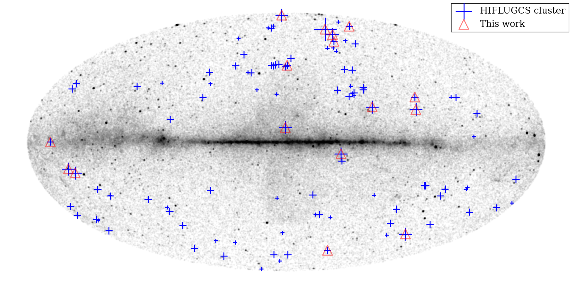
Figure 1: Hammer-Aitoff projection (in Galactic coordinates) of the Fermi-LAT counts map above $10\,\mathrm{GeV}$ for 5 years of LAT exposure. Blue crosses represent the position of the 106 GCls that are contained in the extended HIFLUCGS catalog with the cross size proportional to $\log_{10}{M_{200}/D_{L}^{2}}$ of the GCl (larger crosses being more massive, nearby systems), where $D_{L}$ refers to the luminosity distance in units of Mpc. The colored red triangles indicate the targets used in this study.

Since the predicted number of photons from astrophysical backgrounds is small, and we can localize the signal with its expected spatial information, the primary concern when determining the ROIs surrounding each GCl is to avoid overlap. Performing a joint likelihood with overlapping signal regions can lead to over-estimation of significance [49, 31]. There are infinite combinations of angular radii $R$ which yield a non-overlapping set of ROIs, so we must impose an additional constraint. Because we only model the central target in each fit, expected DM emission from nearby GCls is considered background. We therefore choose to require that our set of ROIs maximizes the ratio of total target emission to nearby GCl contamination. Switching between boost scenarios changes the relative GCl DM emission levels and results in two unique sets of optimal ROI. The respective values of $R$ for each ROI and each substructure scenario, $R_{\mathrm{opt}}$ (optimistic) and $R_{\mathrm{cons}}$ (conservative), along with other GCl parameters are summarized in Table 1.

GCl	$\alpha_{2000}$	$\delta_{2000}$	$z$	$M_{200}$	$R_{200}$	$\theta_{200}$	$c_{200}$	${J_{\mathrm{NFW}}}$	$b_{\mathrm{cons}}$	$b_{\mathrm{opt}}$	$R_{\mathrm{cons}}$	$R_{\mathrm{opt}}$
	(∘)	(∘)		($10^{14}\,M_{\odot}$)	(Mpc)	(∘)		($\mathrm{GeV^{2}\,cm^{-5}}$)			(∘)	(∘)
3C 129	72.29	45.01	0.021	5.90	1.78	1.12	5.030	16.19	34	922	6.0	5.8
A 1060	159.20	-27.53	0.013	2.72	1.37	1.38	5.180	16.38	32	681	2.6	2.7
A 1367	176.10	19.84	0.022	8.13	1.98	1.19	5.000	16.25	34	1045	3.0	3.0
A 2877	17.45	-45.90	0.025	7.54	1.93	1.02	5.000	16.11	34	1014	9.4	9.9
A 3526	192.20	-41.31	0.011	3.72	1.52	1.80	5.110	16.62	33	770	4.0	2.1
A 3627	243.90	-60.91	0.016	5.38	1.72	1.41	5.050	16.40	34	889	2.5	1.0
AWM7	43.63	41.59	0.017	5.38	1.72	1.33	5.050	16.35	34	889	1.0	1.3
Coma	195.00	27.98	0.023	10.92	2.18	1.25	4.970	16.30	35	1172	6.2	3.3
Fornax	54.63	-35.45	0.005	1.39	1.10	2.84	5.350	17.02	30	525	5.2	3.1
M 49	187.40	8.00	0.003	0.72	0.88	3.79	5.580	17.27	28	405	1.5	1.6
NGC 4636	190.70	2.69	0.003	0.19	0.56	2.43	6.150	16.88	23	240	1.2	1.7
NGC 5813	225.30	1.70	0.007	0.46	0.76	1.40	5.750	16.40	26	340	0.5	0.1
Ophiuchus	258.10	-23.38	0.028	42.44	3.43	1.63	5.020	16.55	36	1990	5.0	3.1
Perseus	49.65	41.52	0.018	6.66	1.85	1.35	5.020	16.37	34	966	1.4	1.1
S 636	157.50	-35.32	0.009	1.69	1.17	1.69	5.300	16.56	30	566	3.5	2.7
Virgo	187.70	12.34	0.004	5.60	1.70	6.28	4.210	17.41	34	1299	1.0	0.5

Table 1: List of GCl parameters. The columns from left to right are: right ascension and declination in J2000 epoch, redshift, mass contained in virial radius $R_{200}$, angular radius, $\theta_{200}$, NFW halo concentration parameter, integrated $J$-factor for a smooth NFW halo (logarithm), boost factor for conservative and optimistic substructure models and the associated individually optimized radii for each ROI according to the prediction from the substructure model. We derive both $M_{200}$ and $R_{200}$ from the reported values for $M_{500}$ and $R_{500}$ from the HIFLUGCS catalog [47, 48] and assuming a value of the concentration parameter $c_{200}$, given by the model of [24]. The mass of Virgo is taken from [50].

2.5 Joint Likelihood

Following the precedent set by the Fermi-LAT Collaboration’s searches for DM in dwarf galaxies ([51], [52]), we maximize our sensitivity by combining the information from multiple targets in a joint likelihood.

Beginning with each individual target, we compute the unbinned Poisson likelihood as

$$\mathcal{L}_{t}(\boldsymbol{\mu},\boldsymbol{\theta}_{t}|\mathcal{D}_{t})=\exp{\left({-\int\int\lambda~{}dE~{}dr}\right)}\prod_{i}\lambda(\boldsymbol{r}_{i},E_{i}).$$ (2.4)

In the above equation we introduced $\lambda$, the count-distribution function for all observed photons, as the product of $\boldsymbol{\mu}$ (our parameters of interest, $\boldsymbol{\mu}=\{m_{\mathrm{DM}},\langle\sigma v\rangle_{\gamma\gamma}\}$) and $\boldsymbol{\theta}$ (the list of nuisance parameters $\boldsymbol{\theta}_{t}=\{n_{b,t},\Gamma_{t},\boldsymbol{n}_{\mathrm{src},t}\})$. The integrals cover the ROI and energy window, respectively. We label the normalizations of the background sources $\boldsymbol{n}_{\mathrm{src}}$, diffuse background $n_{b}$, as well as the power-law index for the diffuse background Gamma, with an index $t$ to indicate that these quantities vary and are determined for each target individually. We calculate $\lambda$ by summing our model components (i.e. background source normalizations, power-law spectral index and normalization as well as the normalization of the DM target), each convolved with the exposure and instrument response functions. We find the maximum likelihood $\mathcal{L}_{t}(\boldsymbol{\mu},\hat{\boldsymbol{\theta}}_{t}|\mathcal{D}_{t})$ with respect to the nuisance background parameters and define the joint likelihood as the product over each individual target likelihood, $\mathcal{L}_{t}$:

$$\mathcal{L}_{\mathrm{joint}}(\boldsymbol{\mu}|\boldsymbol{\mathcal{D}})=\prod_{t}\mathcal{L}_{t}(\boldsymbol{\mu},\hat{\boldsymbol{\theta}}_{t}|\mathcal{D}_{t}).$$ (2.5)

Our measure of significance is the test statistic (TS),

$$\mathrm{TS}=2~{}\text{ln}\left(\frac{\mathcal{L}_{\mathrm{joint}}(\hat{\boldsymbol{\mu}}|\boldsymbol{\mathcal{D}})}{\mathcal{L}_{\mathrm{joint}}(\boldsymbol{\mu}_{0}|\boldsymbol{\mathcal{D}})}\right),$$ (2.6)

or twice the difference in log-likelihood between the best-fit and null ($\langle\sigma\nu\rangle_{\gamma\gamma}=0$) hypotheses. According to the asymptotic theorem of Chernoff [53], for fixed WIMP mass, the TS should be $\chi^{2}$-distributed with a single degree of freedom (we scan over a series of fixed values of $m_{\mathrm{DM}}$ with $\langle\sigma\nu\rangle_{\gamma\gamma}$ being the only free parameter), and we set our confidence intervals accordingly. For global significance, the DM mass and the boost setup become free parameters, increasing the degrees of freedom and trials factor. We assess both coverage and global significance through Monte-Carlo (MC) experiments and outline these results in Section 3.

$\mathcal{L}_{\mathrm{joint}}$ could in principle be comprised of every possible GCl with no loss of sensitivity. Targets from which we expect little to no flux are insensitive to changes in $\boldsymbol{\mu}$ and cancel out of the TS. However, to minimize both ROI overlap and computational burden, we form $\mathcal{L}_{\mathrm{joint}}$ with a truncated set. We then compute TS as a function of the cumulative set for ten MC experiments that include a very strong ($\langle\sigma\nu\rangle_{\gamma\gamma}=1.1\times 10^{-22}\mathrm{cm^{3}\,s^{-1}}$) simulated line at 133 $\mathrm{GeV}$. We place a cut at 16 targets (see Fig. 2), where more GCls would only contribute insignificantly to the TS.

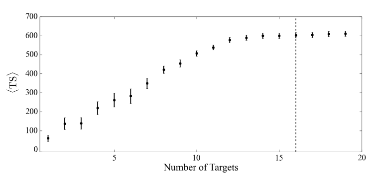
Figure 2: Evolution of the mean joint TS value derived from the combined analysis of GCls (in order of decreasing J-factor). Based on ten simulations with the conservative boost factor setup and a $\langle\sigma\nu\rangle_{\gamma\gamma}=1.1\times 10^{-22}\mathrm{cm^{3}\,s^{-1}}$ for a 133 $\mathrm{GeV}$ monochromatic line with a background model comprised of large-scale diffuse emission templates and 3FGL catalog sources, respectively. The dashed line indicates the number of targets used in this analysis. Injecting a signal with lower $\langle\sigma\nu\rangle_{\gamma\gamma}$ causes the TS to plateau earlier.

3 Performance and Systematic Uncertainties

3.1 Monte-Carlo Performance

We set our significance and confidence interval for each value of $m_{\mathrm{DM}}$ under the assumption that the TS is distributed according to the asymptotic theorem around the maximum likelihood estimate of $\langle\sigma\nu\rangle_{\gamma\gamma}$. A test of this assumption is warranted, in particular, given our simplified background model and the fact that many of our energy windows contain very few or even zero counts. To do this, we simulate a representative background which includes structured Galactic diffuse, isotropic, and point source emission. By performing our analysis on a set of these simulations we calibrate our significance threshold. Then, following the spatial templates described in Section 2.3, we add DM lines resulting from a variety of $\langle\sigma\nu\rangle_{\gamma\gamma}$ to the simulation and assess our sensitivity and coverage.

To determine the null distribution, and thus calibrate our significance, we perform a set of 500 background-only MC experiments for all 16 of our targets. For each one, we extract the maximum significance ($\mathrm{s}_{\mathrm{max}}=\sqrt{\rm TS}$) from all energy windows and both optimistic and conservative boost scenarios. The resulting distribution is depicted in Figure 3.

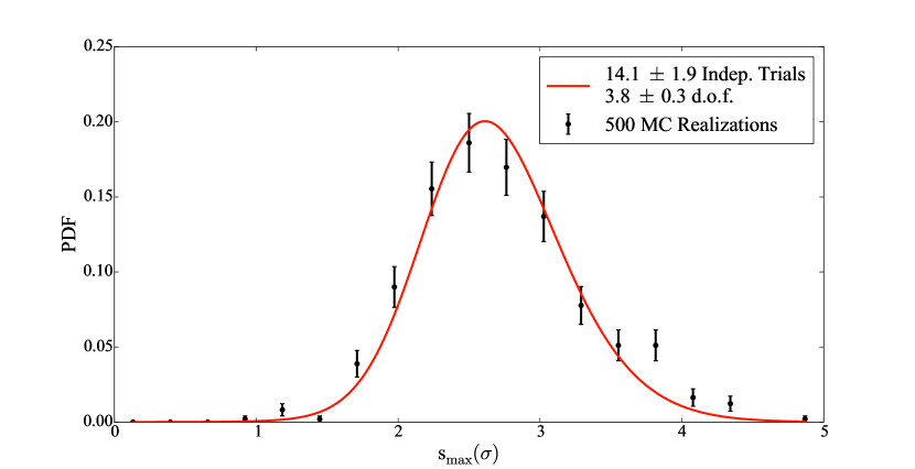
Figure 3: Probability distribution function (PDF) of maximum local significance ($s_{\mathrm{max}}=\sqrt{\mathrm{TS}}$) over all masses and boost scenarios for 500 MC experiments. Fit with a trial-corrected $\chi^{2}$ function, Eq. (3.1).

To convert local to global significances we fit this with a trial-corrected $\chi^{2}$ distribution with both a free number of bounded degrees of freedom $k$, and trials $n_{t}$ [25]:

$$f(\mathrm{s}_{\mathrm{max}})\equiv\frac{d}{dx}\rm CDF(\chi^{2}_{k};x)^{n_{t}}$$ (3.1)

CDF here means the cumulative distribution function. The best-fitting parameters are $k=3.8\pm 0.3$ and $n_{t}=14.1\pm 1.9$.

Using the calibration of global significance, we gauge our sensitivity to a weak DM signal, equivalent to the HRT13 claim. To simulate this, we begin with a signal model which uses the spatial distribution and relative J-factor weighting of our conservative setup. We then tune the value of $\langle\sigma\nu\rangle_{\gamma\gamma}$ such that the total expected counts, including background, matches that reported in HRT13. We perform 10 MC experiments, keeping the total counts fixed, and find that we detect the feature with a local (global) significance of $4.0\pm 0.6\sigma$ ($2.4\pm 0.7\sigma$).

To confirm that our technique yields proper coverage, we further simulate lines for $\langle\sigma\nu\rangle_{\gamma\gamma}$ ranging from $3\times 10^{-26}$ to $1\times 10^{-21}$ cm³ s^-1. To make the calculation feasible, we perform 100 MC experiments for each line using only the four highest J-factor targets, and set joint upper limits. At high $\langle\sigma\nu\rangle_{\gamma\gamma}$, we recover the expected 95% containment. Below a certain threshold in signal strength, however, we expect over-coverage as the sources predict no photons. This occurs at approximately $3\times 10^{-25}\mathrm{cm^{3}\,s^{-1}}$ (again for the conservative boost setup), and below that our method rises to 100% coverage. We conclude that our confidence intervals are conservative where they are not accurate.

3.2 Systematics

In this analysis we make use of the approximate representation of the LAT response via the IRFs. In order to assess how our results are affected by the uncertainties in both point spread function and effective area, we repeat our baseline calculation for the conservative setup but use custom IRFs that bracket the associated uncertainties. These IRFs represent the minimal or maximal variations in the computation of the effective area and PSF within the systematic uncertainties of our chosen IRF (P7REP_CLEAN_V16). Specifically, these IRFs are chosen to maximize and minimize effective area and PSF, respectively (c.f. [33] for details on the bracketing of PSF and effective area, respectively). Previous searches for $\gamma$-ray lines have shown that the uncertainties associated with the energy dispersion are much smaller than the statistical uncertainties of the analysis we report here [28, 30]. Hence we neglect this uncertainty in our bracketing IRF approach. The effect on our upper limits is minor, ranging between 10–20%, with no obvious trend in energy. TS increases when all targets prefer the same value of the joint parameter, $\langle\sigma\nu\rangle_{\gamma\gamma}$. Since the expected flux in Equation 1.1 also depends degenerately on J-factor, TS is sensitive to this relative weighting of targets. We explore our sensitivity to this fact by calculating $\mathrm{s}_{\mathrm{max}}$ for both the HRT13-like signal simulations, and our LAT data, using identical J-factors for each target. We find our local significance to be affected on average by $0.2\pm 0.2\sigma$, with a largest individual change of $-1.2\sigma$ (compared with the conservative J-factor result) at $m_{\mathrm{DM}}=52~{}\mathrm{GeV}$.

A potential additional background source in each of the clusters is its brightest cluster galaxy (BCG). In some clusters, individual cluster member galaxies have been detected in $\gamma$ rays (e.g. NGC 1275 in Perseus [55] or M87 in Virgo [56]). However, searches for $\gamma$-ray emission from a sample of 114 radioselected BCGs have only yielded null results [57]. Even though the sample studied in [57] differs from the one presented in this paper, we can use the observed average flux limit from [57] to derive a conservative estimate of the BCG flux within our energy (and time) range. We find $\overline{F}_{\gamma,\mathrm{BCG}}(E>10\mathrm{GeV})\lesssim 2.0\times 10^{-12}\,\mathrm{ph\,cm^{-2}\,s^{-1}}$. This flux upper limit is comparable to the constraints on diffuse $\gamma$-ray emission $\overline{F}_{\gamma,\mathrm{ICM}}(E>10\mathrm{GeV})\lesssim 2.7\times 10^{-12}\,\mathrm{ph\,cm^{-2}\,s^{-1}}$ [49], as it is expected from cosmic-ray interactions in the intracluster medium (ICM) of the galaxy clusters [23, 58]. The sum of these two contributions amounts to less than 0.1% of the isotropic $\gamma$-ray background flux measured by the LAT in each ROI [59]. Converting these flux limits into photon counts, we find that the combined contribution corresponds to a total of $\sim 20$ photons for the entire sample (with Virgo being the dominant cluster contributing $\sim 8$ photons). Note that both scenarios (BCG and cosmic-ray induced $\gamma$-ray emission) assume a power-law like spectrum, in which case the dominant contribution would be expected towards the lowest energies and thus negligible compared to the observed number of photons in all ROIs (c.f. Fig. 4).

4 Results

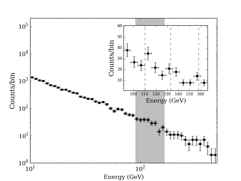
Figure 4: Shown is the stacked spectrum from photons sub-selected within each optimal radius of the 16 clusters analyzed in this work. The inset shows a zoom in the energy window (light-gray shaded area) that coincides with the discussed line signals at 110, 133, and 158 $\mathrm{GeV}$, respectively (dashed-gray lines). Note that displaying the data as stack of binned histograms is for visualization purposes only, while the underlying analysis employs an unbinned joint likelihood method (see text).

Applying our analysis to a five-year dataset, we observe no significant excess over the energy range from 10 to 400 GeV and place 95% confidence upper limits on $\langle\sigma\nu\rangle_{\gamma\gamma}$. The limits are plotted in Fig. 5 for both boost scenarios, along with 68/95% bands containing background-only MC limits.

Figure 5: Observed 95% confidence upper limits for both conservative (left) and optimistic (right) boost scenarios. Yellow and green bands represent 68% and 95% containment of limits obtained by MC simulations. Note that the upper limits and TS are not always correlated – the upper limit value by itself gives no information about the relative likelihoods of the null and best-fit hypotheses.

The stacked spectrum of all included photons can be seen in Fig. 4. The highest local significance occurs for the optimistic setup at 75 $\mathrm{GeV}$ with a value of $1.5\sigma$, corresponding globally to $<0.1\sigma$. These results are in agreement with recent updates on the GC [28, 30], which also find no significant line emission.

It should be noted that the most recent of these GC studies [30], utilized a new data set (Pass 8) which benefits from an improved instrument acceptance and PSF. Performing our analysis with 6 years of P8_SOURCE_V6 data set yields results qualitatively compatible to those from Pass 7 reprocessed (this work), with a maximum local significance of $1.5\sigma$ at 181 $\mathrm{GeV}$. Determining the global significance would require repeating the studies of §3, and would yield a lower value. We also neglected to take advantage of a new feature, known as event types, which subdivide the data based on the uncertainty of the energy reconstruction and provide corresponding IRFs. Although this could have improved our sensitivity by approximately 15% [30], the lack of significant features in the data did not warrant its implementation.

4.1 The Feature at $\mathbf{133\,\mathrm{\mathbf{GeV}}}$ and Double Lines

Although within the 95% containment band expected from random background fluctuations, we note two upturns (around 133 GeV and 158 GeV) in both our observed limits between the energies of 100 and 200 $\mathrm{GeV}$. If the 133 GeV feature is indeed of the same origin as previously been seen in the GC [25, 28], where statistical fluctuations in Pass 7 data seem to have played a major role [30], we expect to see a significant decrease in TS since the HRT13 claim. Repeating our analysis with exposure periods of two, three and four years, respectively, we find the $\sim 133\,\mathrm{GeV}$ feature to decrease monotonically from $\mathrm{TS}\simeq 1.8$ with 2 years of exposure to $\mathrm{TS}\simeq 0.3$ with five years.

Inspired by the the HRT13 statements of a potential double peaked feature, from a $\sim$110 GeV and $\sim$130 GeV line, we also investigated if such a setup could increase the TS. With slightly wider energy windows, we repeat our analysis for the conservative boost scenario with a second lower energy line together with a 133 GeV line. We vary the relative intensity and take various energies of a second line around 110 GeV. We test 110 GeV as well as 106 GeV and 120 GeV, where the latter two energies are the expected energies if a 133 GeV line from DM annihilates into $\gamma\gamma$ is adjoined with a second line from $\gamma h$ or $\gamma Z$ final state, respectively. The TS for such double lines stays below $1$ in our joint-cluster analysis, and we conclude that with our analysis setup we see no significant single nor double line associated with a 133 GeV line. Similarly, we tested for a double line at 158 GeV and 133 GeV. These energies coincide with our observed two bumps in cross-section limits and can be theoretically expected if the DM particles annihilate into $\gamma\gamma$ and $\gamma h$. Such a double line can give a TS of 1.7, which is however still not statistically significant (especially if taking into account the “look elsewhere” penalty and that a larger energy window is used).F

5 Discussion and Conclusions

A detection of a monochromatic $\gamma$-ray line from the most massive and nearby GCls would be extremely intriguing. The prime candidate for causing such a signal could only be the existence of DM particle annihilations or decays.

After a tentative line-like feature at 133 GeV has been reported in Fermi-LAT data in the GC region [25, 27], evidence was also presented that it was seen in GCls (HRT13). In some DM particle models such strong line-like feature can indeed be expected in this energy region (see, e.g., [8, 7, 60, 14, 61, 62, 63, 64]). Moreover, if a DM annihilation signal is confirmed towards GCls it would not only reveal important properties of the DM particle but also about how DM clusters — a detectable $\gamma$-ray line signal in GCls can namely only be excepted if a large number of highly concentrated DM substructures exist down to small halo masses.

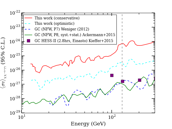
Figure 6: Comparison of results presented in this work with other line searches; we only consider works in which constraints on $\langle\sigma\nu\rangle_{\gamma\gamma}$ were calculated that overlap with the energy range used here. Green-solid and Blue-dashed lines correspond to results obtained analyzing data from the GC assuming an NFW profile using LAT data [25, 30] while the squared markers correspond to recently published preliminary observed limits from 2.8 hours of observing the GC with the H.E.S.S. II telescope [65]. The gray-dashed vertical line corresponds to the energy at which the initial excess was reported $\sim 130\,\mathrm{GeV}$.

Subsequent Fermi-LAT data have revealed that the statistical significance has dropped for the $\sim$133 GeV line signal from the GC [66, 30]. In this study we analyzed 5 years of Pass 7 reprocessed data to scrutinize the auxiliary support of the line feature from GCls. We find no remaining indications of a monochromatic $\gamma$-ray line in our stacked cluster analysis. For different J-factor assumptions, we instead derive upper bounds on DM annihilation cross sections for DM masses in the range from 10 to 400 GeV. These limits (see Fig. 6 for a comparison) are weaker than those derived from the Galactic $\gamma$-ray line search program by the Fermi-LAT collaboration [67, 68, 28, 30], but they nevertheless constitute a very important complementary probe as long as the nature and clustering properties of the DM remain unknown.

References

- [1] D. Clowe, M. Bradač, A. H. Gonzalez, M. Markevitch, S. W. Randall, C. Jones, and D. Zaritsky, A Direct Empirical Proof of the Existence of Dark Matter, ApJ 648 (Sept., 2006) L109–L113, [astro-ph/0608407].
- [2] F. Combes, Properties of dark matter haloes, New A Rev. 46 (Nov., 2002) 755–766, [astro-ph/0206126].
- [3] G. Bertone, D. Hooper, and J. Silk, Particle dark matter: evidence, candidates and constraints, Phys. Rep. 405 (Jan., 2005) 279–390, [hep-ph/0404175].
- [4] J. Einasto, Dark Matter, ArXiv e-prints (Jan., 2009) [arXiv:0901.0632].
- [5] J. L. Feng, Dark Matter Candidates from Particle Physics and Methods of Detection, ARA&A 48 (Sept., 2010) 495–545, [arXiv:1003.0904].
- [6] L. Bergström, Non-baryonic dark matter: observational evidence and detection methods, Reports on Progress in Physics 63 (May, 2000) 793–841, [hep-ph/0002126].
- [7] L. Bergstrom, Dark Matter Candidates, New J.Phys. 11 (2009) 105006, [arXiv:0903.4849].
- [8] L. Bergström and H. Snellman, Observable monochromatic photons from cosmic photino annihilation, Phys. Rev. D 37 (June, 1988) 3737–3741.
- [9] S. Rudaz, Annihilation of heavy-neutral-fermion pairs into monochromatic rays and its astrophysical implications, Phys. Rev. D 39 (June, 1989) 3549–3556.
- [10] G. F. Giudice and K. Griest, Rate for annihilation of galactic dark matter into two photons, Phys. Rev. D 40 (Oct., 1989) 2549–2558.
- [11] L. Bergström and P. Ullio, Full one-loop calculation of neutralino annihilation into two photons, Nuclear Physics B 504 (Feb., 1997) 27–44, [hep-ph/9706232].
- [12] S. Matsumoto, J. Sato, and Y. Sato, Enhancement of Line Gamma Ray Signature from Bino-like Dark Matter Annihilation due to CP Violation, ArXiv High Energy Physics - Phenomenology e-prints (May, 2005) [hep-ph/0505160].
- [13] F. Ferrer, L. M. Krauss, and S. Profumo, Indirect detection of light neutralino dark matter in the next-to-minimal supersymmetric standard model, Phys. Rev. D 74 (Dec., 2006) 115007, [hep-ph/0609257].
- [14] M. Gustafsson, E. Lundström, L. Bergström, and J. Edsjö, Significant Gamma Lines from Inert Higgs Dark Matter, Physical Review Letters 99 (July, 2007) 041301, [astro-ph/0703512].
- [15] S. Profumo, Hunting the lightest lightest neutralinos, Phys. Rev. D 78 (July, 2008) 023507, [arXiv:0806.2150].
- [16] J. Conrad, Statistical issues in astrophysical searches for particle dark matter, Astroparticle Physics 62 (Mar., 2015) 165–177, [arXiv:1407.6617].
- [17] S. Zimmer, J. Conrad, for the Fermi-LAT Collaboration, and A. Pinzke, A Combined Analysis of Clusters of Galaxies - Gamma Ray Emission from Cosmic Rays and Dark Matter, ArXiv e-prints (Oct., 2011) [arXiv:1110.6863].
- [18] X. Huang, G. Vertongen, and C. Weniger, Probing dark matter decay and annihilation with Fermi LAT observations of nearby galaxy clusters, J. Cosmology Astropart. Phys. 1 (Jan., 2012) 42, [arXiv:1110.1529].
- [19] S. Ando and D. Nagai, Fermi-LAT constraints on dark matter annihilation cross section from observations of the Fornax cluster, J. Cosmology Astropart. Phys. 7 (July, 2012) 17, [arXiv:1201.0753].
- [20] R. D. Griffin, X. Dai, and C. S. Kochanek, New Limits on Gamma-Ray Emission from Galaxy Clusters, ApJ 795 (Nov., 2014) L21, [arXiv:1405.7047].
- [21] V. Springel, J. Wang, M. Vogelsberger, A. Ludlow, A. Jenkins, A. Helmi, J. F. Navarro, C. S. Frenk, and S. D. M. White, The Aquarius Project: the subhaloes of galactic haloes, MNRAS 391 (Dec., 2008) 1685–1711, [arXiv:0809.0898].
- [22] M. Kuhlen, The Dark Matter Annihilation Signal from Dwarf Galaxies and Subhalos, Advances in Astronomy 2010 (2010) 45, [arXiv:0906.1822].
- [23] A. Pinzke, C. Pfrommer, and L. Bergström, Prospects of detecting gamma-ray emission from galaxy clusters: Cosmic rays and dark matter annihilations, Phys. Rev. D 84 (Dec., 2011) 123509, [arXiv:1105.3240].
- [24] M. A. Sánchez-Conde and F. Prada, The flattening of the concentration-mass relation towards low halo masses and its implications for the annihilation signal boost, MNRAS 442 (Aug., 2014) 2271–2277, [arXiv:1312.1729].
- [25] C. Weniger, A tentative gamma-ray line from Dark Matter annihilation at the Fermi Large Area Telescope, J. Cosmology Astropart. Phys. 8 (Aug., 2012) 7, [arXiv:1204.2797].
- [26] E. Tempel, A. Hektor, and M. Raidal, Fermi 130 GeV gamma-ray excess and dark matter annihilation in sub-haloes and in the Galactic centre, J. Cosmology Astropart. Phys. 9 (Sept., 2012) 32, [arXiv:1205.1045].
- [27] M. Su and D. P. Finkbeiner, Strong Evidence for Gamma-ray Line Emission from the Inner Galaxy, ArXiv e-prints (June, 2012) [arXiv:1206.1616].
- [28] Fermi-LAT Collaboration, M. Ackermann et al., Search for gamma-ray spectral lines with the Fermi Large Area Telescope and dark matter implications, Phys. Rev. D 88 (Oct., 2013) 082002.
- [29] A. Hektor, M. Raidal, and E. Tempel, Evidence for Indirect Detection of Dark Matter from Galaxy Clusters in Fermi -Ray Data, ApJ 762 (Jan., 2013) L22, [arXiv:1207.4466].
- [30] Fermi-LAT Collaboration, Ackermann, M. and others, Updated Search for Spectral Lines from Galactic Dark Matter Interactions with Pass 8 Data from the Fermi Large Area Telescope, ArXiv e-prints (May, 2015) [arXiv:1506.00013].
- [31] B. Anderson, J. Chiang, J. Cohen-Tanugi, J. Conrad, A. Drlica-Wagner, M. Llena Garde, and S. Zimmer for the Fermi-LAT Collaboration, Using Likelihood for Combined Data Set Analysis, ArXiv e-prints (Feb., 2015) [arXiv:1502.03081].
- [32] Fermi-LAT Collaboration, W. B. Atwood et al., The Large Area Telescope on the Fermi Gamma-ray Space Telescope Mission, Astrophys. J. 697 (2009) 1071–1102, [arXiv:0902.1089].
- [33] Fermi-LAT Collaboration, M. Ackermann et al., The Fermi Large Area Telescope on Orbit: Event Classification, Instrument Response Functions, and Calibration, ApJS 203 (Nov., 2012) 4, [arXiv:1206.1896].
- [34] Fermi-LAT Collaboration, F. Acero et al., Fermi Large Area Telescope Third Source Catalog, ApJS 218 (June, 2015) 23, [arXiv:1501.02003].
- [35] A. V. Kravtsov and S. Borgani, Formation of Galaxy Clusters, ARA&A 50 (Sept., 2012) 353–409, [arXiv:1205.5556].
- [36] J. Lavalle, Q. Yuan, D. Maurin, and X.-J. Bi, Full calculation of clumpiness boost factors for antimatter cosmic rays in the light of CDM N-body simulation results. Abandoning hope in clumpiness enhancement?, A&A 479 (Feb., 2008) 427–452, [arXiv:0709.3634].
- [37] J. F. Navarro, C. S. Frenk, and S. D. M. White, A Universal Density Profile from Hierarchical Clustering, ApJ 490 (Dec., 1997) 493, [astro-ph/9611107].
- [38] L. Gao, J. F. Navarro, C. S. Frenk, et al., The phoenix project: the dark side of rich galaxy clusters, MNRAS 425 (Jan., 2012) 2169, [arXiv:1201.1940].
- [39] W. A. Hellwing, C. S. Frenk, M. Cautun, S. Bose, J. Helly, A. Jenkins, T. Sawala, and M. Cytowski, The Copernicus Complexio: a high-resolution view of the small-scale Universe, ArXiv e-prints (May, 2015) [arXiv:1505.06436].
- [40] D. Anderhalden and J. Diemand, Density profiles of CDM microhalos and their implications for annihilation boost factors, J. Cosmology Astropart. Phys. 4 (Apr., 2013) 9, [arXiv:1302.0003].
- [41] T. Ishiyama, Hierarchical Formation of Dark Matter Halos and the Free Streaming Scale, ApJ 788 (June, 2014) 27, [arXiv:1404.1650].
- [42] A. M. Green, S. Hofmann, and D. J. Schwarz, The power spectrum of SUSY-CDM on subgalactic scales, MNRAS 353 (Sept., 2004) L23–L27, [astro-ph/0309621].
- [43] S. Profumo, K. Sigurdson, and M. Kamionkowski, What Mass Are the Smallest Protohalos?, Physical Review Letters 97 (July, 2006) 031301, [astro-ph/0603373].
- [44] T. Bringmann, Particle models and the small-scale structure of dark matter, New Journal of Physics 11 (Oct., 2009) 105027, [arXiv:0903.0189].
- [45] A. D. Ludlow, J. F. Navarro, R. E. Angulo, M. Boylan-Kolchin, V. Springel, C. Frenk, and S. D. M. White, The mass-concentration-redshift relation of cold dark matter haloes, MNRAS 441 (June, 2014) 378–388, [arXiv:1312.0945].
- [46] M. A. Sánchez-Conde, M. Cannoni, F. Zandanel, et al., Dark matter searches with Cherenkov telescopes: nearby dwarf galaxies or local galaxy clusters?, J. Cosmology Astropart. Phys. 12 (Dec., 2011) 11, [arXiv:1104.3530].
- [47] T. H. Reiprich and H. Böhringer, The Mass Function of an X-Ray Flux-limited Sample of Galaxy Clusters, ApJ 567 (Mar., 2002) 716–740, [astro-ph/0].
- [48] Y. Chen, T. H. Reiprich, H. Böhringer, et al., Statistics of X-ray observables for the cooling-core and non-cooling core galaxy clusters, A&A 466 (May, 2007) 805–812, [astro-ph/0].
- [49] Fermi-LAT Collaboration, M. Ackermann et al., Search for Cosmic-Ray-induced Gamma-Ray Emission in Galaxy Clusters, ApJ 787 (May, 2014) 18, [arXiv:1308.5654].
- [50] P. Fouqué, J. M. Solanes, T. Sanchis, and C. Balkowski, Structure, mass and distance of the Virgo cluster from a Tolman-Bondi model, A&A 375 (Sept., 2001) 770–780, [astro-ph/0106261].
- [51] Fermi-LAT Collaboration, M. Ackermann et al., Constraining Dark Matter Models from a Combined Analysis of Milky Way Satellites with the Fermi Large Area Telescope, Physical Review Letters 107 (Dec., 2011) 241302, [arXiv:1108.3546].
- [52] Fermi-LAT Collaboration, M. Ackermann et al., Dark Matter Constraints from Observations of 25 Milky Way Satellite Galaxies with the Fermi Large Area Telescope, ArXiv e-prints (Oct., 2013) [arXiv:1310.0828].
- [53] H. Chernoff, A Measure of Asymptotic Efficiency for Tests of a Hypothesis Based on the sum of Observations, The Annals of Mathematical Statistics 23 (Dec., 1952) 493–507.
- [54] E. Gross and O. Vitells, Trial factors for the look elsewhere effect in high energy physics, European Physical Journal C 70 (Nov., 2010) 525–530, [arXiv:1005.1891].
- [55] MAGIC Collaboration, J. Aleksić et al., Detection of very-high energy -ray emission from NGC 1275 by the MAGIC telescopes, A&A 539 (Mar., 2012) L2, [arXiv:1112.3917].
- [56] Fermi-LAT Collaboration, A. A. Abdo et al., Fermi Large Area Telescope Gamma-Ray Detection of the Radio Galaxy M87, ApJ 707 (Dec., 2009) 55–60, [arXiv:0910.3565].
- [57] K. L. Dutson, R. J. White, A. C. Edge, J. A. Hinton, and M. T. Hogan, A stacked analysis of brightest cluster galaxies observed with the Fermi Large Area Telescope, MNRAS 429 (Mar., 2013) 2069–2079, [arXiv:1211.6344].
- [58] F. Zandanel and S. Ando, Constraints on diffuse gamma-ray emission from structure formation processes in the Coma cluster, MNRAS 440 (May, 2014) 663–671, [arXiv:1312.1493].
- [59] Fermi-LAT Collaboration, M. Ackermann et al., The Spectrum of Isotropic Diffuse Gamma-Ray Emission between 100 MeV and 820 GeV, ApJ 799 (Jan., 2015) 86.
- [60] J. Hisano, S. Matsumoto, and M. M. Nojiri, Explosive dark matter annihilation, Phys.Rev.Lett. 92 (2004) 031303, [hep-ph/0307216].
- [61] C. Jackson, G. Servant, G. Shaughnessy, T. M. Tait, and M. Taoso, Higgs in Space!, JCAP 1004 (2010) 004, [arXiv:0912.0004].
- [62] E. Dudas, Y. Mambrini, S. Pokorski, and A. Romagnoni, Extra U(1) as natural source of a monochromatic gamma ray line, JHEP 1210 (2012) 123, [arXiv:1205.1520].
- [63] X. Chu, T. Hambye, T. Scarna, and M. H. Tytgat, What if Dark Matter Gamma-Ray Lines come with Gluon Lines?, Phys.Rev. D86 (2012) 083521, [arXiv:1206.2279].
- [64] M. R. Buckley and D. Hooper, Implications of a 130 GeV Gamma-Ray Line for Dark Matter, Phys.Rev. D86 (2012) 043524, [arXiv:1205.6811].
- [65] M. Kieffer, K. Dundas Mora, J. Conrad, C. Farnier, A. Jacholkowska, J. Veh, A. Viana, and for the H. E. S. S. Collaboration, Search for Gamma-ray Line Signatures with H.E.S.S, ArXiv e-prints (Sept., 2015) [arXiv:1509.03514].
- [66] M. Gustafsson for the Ferm-LAT Collaboration, Fermi-LAT and the Gamma-Ray Line Search, arXiv:1310.2953.
- [67] Fermi-LAT Collaboration, A. Abdo et al., Fermi LAT Search for Photon Lines from 30 to 200 GeV and Dark Matter Implications, Phys.Rev.Lett. 104 (2010) 091302, [arXiv:1001.4836].
- [68] Fermi-LAT Collaboration, M. Ackermann et al., Fermi LAT Search for Dark Matter in Gamma-ray Lines and the Inclusive Photon Spectrum, Phys.Rev. D86 (2012) 022002, [arXiv:1205.2739].